
Submitted:
16 October 2024
Posted:
17 October 2024
You are already at the latest version
Abstract
Super-resolution (SR) techniques have shown great promise in enhancing the resolution of MRI images, which are often limited by hardware constraints and acquisition time. Regularization-based methods, which incorporate prior knowledge into the SR process, have been especially effective in improving image quality and mitigating the effects of noise and blur. In this paper, we propose an advanced regularization method for MRI super-resolution that balances high-frequency detail preservation with noise suppression. By leveraging spatially adaptive regularization techniques and a robust denoising process, the proposed method outperforms traditional SR algorithms, as demonstrated on real-world MRI datasets.
Keywords:
MRI
; Super-resolution
; Regularization method
1. Introduction
Super-resolution (SR) has gained significant attention in recent years, particularly in medical imaging applications, where the resolution of acquired images is often limited by hardware constraints, time limitations, and patient comfort considerations. Traditional medical imaging modalities such as Magnetic Resonance Imaging (MRI) and Computed Tomography (CT) produce images at a resolution that can restrict the level of detail observable for diagnostic purposes. Increasing the resolution of these images through hardware improvements is often costly and impractical. As a result, computational techniques like SR have emerged as a powerful alternative, allowing high-resolution (HR) images to be reconstructed from low-resolution (LR) inputs without the need for expensive hardware [1,2,3].
The principle behind SR methods is to overcome limitations by leveraging redundant information from multiple LR images or sequences, often involving complex algorithms like regularization methods and machine learning models [4]. Various approaches, from classic interpolation methods to more advanced neural network-based models, have been employed to enhance the quality of medical images in terms of spatial resolution, signal-to-noise ratio (SNR), and edge preservation [5].
In medical imaging, SR is particularly valuable because it enhances the quality of images used in diagnostic processes. For instance, MRI scans are used to assess various medical conditions, and improving their resolution can lead to more accurate diagnoses. Using SR techniques like Wiener filter regularization [1] or edge-preserving high-frequency regularization [3] allows for better visual quality in images without increasing acquisition costs or hardware requirements. Furthermore, neural network-based SR methods [2] have demonstrated promising results in improving image quality with reduced computational time, making them suitable for real-time applications in clinical settings.
The concept of SR in medical imaging has evolved significantly over the years, with various methodologies proposed to tackle the challenges of resolution enhancement. One of the early applications of SR to MRI was proposed by Peled et al. [6], where an Iterative-Back-Projection (IBP) method was used to enhance MRI images of human white matter fiber tracts. While this method showed some promise, it was limited by the use of synthetic image data, which does not fully capture the complexities of real-world medical imaging. Subsequent work by Scheffler [7] addressed this limitation by highlighting the importance of utilizing original image data for more reliable SR reconstruction.
More recently, the integration of machine learning techniques into SR models has shown great promise. For example, a method combining iterative regularization with feed-forward neural networks was proposed by Babu et al. [2], yielding improved results over previous methods due to its capability to handle noise and produce clearer, higher-resolution images. This method demonstrates the potential of neural networks to enhance SR models by reducing computational complexity while maintaining high image quality.
Bayesian methods have also been a major area of exploration in SR research [8,9,10,11,12]. Aguena et al. [1] introduced a Bayesian approach to MRI SR, which employed a Wiener filter to regularize the iterative solution. This method achieved notable improvements in both noise reduction and edge preservation. Similarly, Ben-Ezra et al. [4] proposed a regularized SR framework for brain MRI, incorporating domain-specific knowledge to improve the quality of SR reconstructions. Their approach outperformed traditional maximum a posteriori (MAP) estimators in terms of both edge clarity and overall image quality.
Moreover, Ahmadi and Salari [3] proposed a high-frequency regularization technique that combines edge-preserving methods with traditional SR models. Their approach allows for enhanced edge definition in MRI images without the need for image segmentation, offering a computationally efficient solution suitable for clinical applications.
The Accelerated Proximal Gradient Method (APGM), as outlined in [13], is a well-known optimization technique commonly used for solving inverse problems in imaging, including SR. APGM accelerates the convergence of proximal gradient methods, which are widely adopted for SR tasks involving regularization. Its primary strength lies in its speed, as it converges more quickly than traditional gradient methods, making it suitable for large-scale imaging problems. However, APGM’s effectiveness is heavily dependent on the choice of regularizer, which influences how well the method can balance smoothness and sharpness in the reconstructed image. Poorly chosen regularizers can introduce artifacts or excessively smooth the image. While APGM is flexible and powerful, it requires careful tuning to achieve optimal results, especially when handling high-frequency details.
Block-matching and 3D filtering (BM3D), a renowned denoising algorithm discussed in [14], uses a collaborative filtering approach to reduce noise while preserving image structures. For super-resolution tasks, BM3D can act as a regularizer that effectively manages noise without compromising edges and textures. Its block-matching mechanism compares similar patches in the image, applying 3D filtering to reduce noise in these matched blocks. Although BM3D excels at preserving textures and fine details in natural images, its computational complexity can be high, particularly when dealing with large images or complex noise patterns. Additionally, the block-matching process may struggle in scenarios where image structures do not align well with the blocks, leading to potential loss of detail in areas with intricate textures.
Gu et al. [15] enhanced the BM3D algorithm by introducing weighted nuclear norm minimization, which improved its performance in image denoising. This modification further solidified BM3D as a versatile and widely adopted tool in image processing. Although BM3D is primarily an image denoising algorithm rather than a typical regularization technique, denoising often relies on regularization to reduce noise and improve image quality. BM3D utilizes collaborative filtering and 3D transform-domain techniques to achieve denoising, making it more aligned with advanced signal processing than conventional regularization methods.
Total variation (TV) regularization, a widely used technique in inverse problems, aims to promote sparsity in image gradients, leading to smoother regions while preserving sharp edges. TV regularization is known for its simplicity and its ability to retain edge information, making it a popular choice in SR tasks. However, TV regularization often suffers from the staircasing effect, where smooth regions of the image appear blocky or exhibit artificial edges. Over-regularization can further result in a loss of fine details, which limits the technique’s applicability in images with rich textures or high-frequency content [16].
Rapid and Accurate Image Super Resolution (RAISR), introduced in [17], is a learning-based SR method that is both computationally efficient and fast. It works by learning filters that are adaptive to local image features, such as gradients and edge orientations. Unlike deep learning-based methods that often require significant computational resources, RAISR is lightweight and quick, making it an attractive option for real-time applications. Despite its efficiency, RAISR tends to fall short when compared to more advanced SR methods like deep neural networks in terms of recovering high-frequency details. Its performance is highly dependent on the quality of the learned filters, and it may struggle with images that have complex structures or varying noise levels.
PPPV1, as described in [18], is a video super-resolution method, based on the Plug-and-Play (PnP) framework. This method iteratively refines images, ensuring the gradual recovery of fine details over multiple iterations. A key feature of PPPV1 is its reliance on a denoising module, originally based on DnCNN (Denoising Convolutional Neural Network), to remove noise from the image during each step of the reconstruction process. While DnCNN is effective at reducing noise, it sometimes introduces oversmoothing, especially in high-frequency regions where texture and fine details are critical. The proposed improvement to this method involves replacing DnCNN with a custom prior for denoising. This change allows for more control over detail preservation and texture recovery, potentially reducing the risk of oversmoothing. A well-designed custom prior can provide better balance between noise suppression and sharpness, which could lead to more accurate and visually appealing results, particularly in areas with intricate patterns or high-frequency details.
In addition to neural network-based and Bayesian approaches, convex optimization methods have been explored. Kawamura et al. [5] applied convex optimization techniques to MRI SR, producing state-of-the-art results by carefully balancing noise suppression and detail preservation.
Overall, the field of SR in medical imaging is rapidly advancing, with numerous approaches showing great potential in improving diagnostic imaging and reducing the need for high-cost imaging hardware. The next phase of research will likely focus on integrating these various techniques into more robust, real-time systems suitable for clinical environments.
In this paper, we propose an improved PPP regularization method for MRI super-resolution, utilizing an effective prior specifically designed for denoising and handling motion between frames. Building upon the foundation of our previous method (PPPV1 [18]), our approach incorporates an innovative denoiser that significantly enhances performance. Unlike traditional methods that primarily focus on denoising, our method integrates these advances into an MRI super-resolution framework.
2. Materials and Methods
The acquisition model we are assuming is:
where:
- is the full set of low resolution (LR) frames, described as , where are the p LR images. Each observed LR image is of size . Let the kth LR image be denoted in lexicographic notation as , for and .
- is the desired high resolution (HR) image, of size , written in lexicographical notation as the vector , where and and represent the up-sampling factors in the horizontal and vertical directions, respectively.
- , where is the noise vector for frame k and contains independent zero-mean Gaussian random variables.
- is the degradation matrix which performs the operations of blur, rigid transformation and subsampling.
Assuming that each LR image is corrupted by additive noise, we can then represent the observation model as [19]:
where
is a matrix of size that performs the rigid transformation, represents a blur matrix, and S is a subsampling matrix. In our case , since we assumed no added blur on video frames.
The goal is to find the estimate of the HR image from the p LR images by minimizing the cost function
where is the “fidelity to the data” term, and is the regularization term, which offers some prior knowledge about . In this study, we adopt the Plug-and-Play Priors approach, in which the ADMM algorithm is modified so that the proximal the proximal operator related to is replaced by a denoiser that solves the problem of Eq. (5). The denoiser used is based on the work by Chantas et al. [20].
The following outlines the algorithm we propose:
- 1.
-
The first step of our algorithm is to evaluate the term from the Equation (3), by using rigid registration. Rigid registration, also known as rigid body registration or rigid transformation, is a fundamental technique in medical image processing and computer vision. It is used to align two images by performing translations and rotations while preserving the shape and size of the structures within the images [22].In a 2D plane, a rigid transformation can be represented using a matrix, often referred to as the transformation matrix. For example, a 2D translation can be represented as [23]:Rotation and reflection matrices can also be formulated similarly. The result of the rigid transformation is represented as an affine transformation matrix. This matrix captures the translation and rotation parameters applied to the original image [23].We assume that one of the LR images, (typically the middle one), is produced from the HR image , by applying only downsampling, without transformation. Thus, . Rigid transformation is calculated between and the rest of the LR images. Following that, we get for the remaining images.
- 2.
- The subsequent phase is centered on employing the PnP-ADMM technique. We execute the PnP-ADMM, adhering to the procedure outlined in Algorithm 1 until reaching convergence, in order to minimize the problem described by Eq. (4). The initial HR image guess, , is generated from using the pseudo-inverse of . Here, D represents the denoising operator, introduced and discussed in Section 2.1, and g is formulated as .
| Algorithm 1 PnP-ADMM [24] |
|
We next explain the modification made to the standard ADMM algorithm to obtain PnP-ADMM. Line 4 or the standard ADMM is . In the PnP-ADMM, the proximal operator is replaced by a denoiser D that solves the problem
It can be shown that the Maximum A Posteriori (MAP) estimator of is the proximal operator:
for .
2.1. The Denoising Algorithm
In this section, we describe the algorithm we use to implement the denoising step of Eq. (6). The algorithm is a simplification of that proposed in [20], it is formulated in a probabilistic (Variational Bayes) context and utilizes an effective prior distribution, which we describe in short next.
2.1.1. The Prior Distribution
The prior distribution we employ for the denoising step was proposed in [20] for single image Super-Resolution, and it is of the form:
where are the real-positive distribution parameters and is a similarity measure between two patches each of center pixel w and . The above distribution is produced after integrating out the hidden variables of the prior in [20]. However, this form in never explicitly used (it is not necessary) in the optimization algorithm. We show it here in this form for simplicity of presentation. Indeed, enables us to interpret the prior in a deterministic context, analogous with the penalty function imposed on the video frames, see equation (6).
We introduce a similarity measure between two image patches, denoted as and , where and represent the central pixel of the first and second patch, respectively.
The complete set of pixel coordinates is represented by . Furthermore, we define as the integer displacement between the center pixels of the two patches, such that . For measuring similarity, we employ a weighted Euclidean norm, represented by , to quantify the difference between and (or ) as follows:
where is defined by: and indicates the vector obtained by squaring each element of . represents the difference operator, an matrix, such that the i-th component of equals for all with . The matrix is an diagonal matrix, where its diagonal elements corresponding to the pixels in are the only non-zero values, specifically, for all i not in . Lastly, we denote by the vector with elements the weights of the weighted norm: the closer to the central pixel of the patches the larger the weight value.
The norm defined by (8) retains its value even if the summation (8) runs over only the subset instead of , since for . However, we use the full summation range over for enabling fast computations with the Fast Fourier Transform, as explained next.
The distance between the patch and an arbitrary patch , , is . Given that the image patches correspond to and , it is:
As we can see, each , is a circularly shifted by version of (denoted simply by from now on). The formula (8) for calculating , expressed in terms of , is:
Clearly, the values of for all w’s, are the result of the correlation between and , since the indices of and always differ by the constant . To calculate the correlation required for the super-resolution technique discussed in the following section, we use the Fast Fourier Transform (FFT). This approach decreases the computational complexity of the algorithm from , typical for correlation calculations, to , which is the complexity for multiplication in the DFT (Discrete Fourier Transform) domain.
2.1.2. Denoising in PnP-ADMM
Next, we describe the algorithm we employ in the PnP-ADMM context of Algorithm 1, and specifically for the denoising step (line 4). The algorithm we employ, as a denoising sub-problem of the general super-resolution algorithm (Algorithm 1), is in essence a special case of the VBPS algorithm in [20], where there is no blurring nor decimation. Mathematically speaking, this means that the imaging operator is the identity matrix , as shown in line 8 of Algorithm 2.
| Algorithm 1: Variational Bayes Patch Similarity Denoising |
|
Input: Noisy image .
Output: Denoised image .
Initialization:
Image initial estimate: Set , where is the regularization parameter obtained from [21]. Then, set , where is the super-resolved image obtained after setting . Parameter selection: Set , and , , , , and err .
|
More specifically, the imaging model assumed for the denoising step is a simplified form of Eq. (2.1) in [20], because it is now (i.e., no blur/decimation, hence it is just the identity matrix). Also, in this form, has the role of the “noisy image” and is the uncorrupted one, meant to be estimated by the denoising algorithm.
In parallel with imaging model, we assume the imaging model, i.e., the prior distribution introduced above and given by Eq. (5). This is in essence the prior distribution for the uncorrupted image to be estimated via the denoising procedure. This means that the Algorithm 2 is the result of the adoption of both the imaging model mentioned above and the prior (5) for . Lastly, note that the denoising Algorithm 2 selects automatically, in the initialization step, the noise variance , among other parameters.
We implemented our method in SCICO [25], which is an open source library for computational imaging that includes implementations of several algorithms.
To evaluate our method, the widely-used publicly available dataset named the cancer image archive (TCIA) [26] was used, in order to compare our results to the previously proposed method. Specifically, we conducted experiments using a dataset of LR brain MRI images and a corresponding HR reference dataset.
3. Results
Our method with the effective prior achieved notable improvements in image quality, as demonstrated by Figure 1 and Figure 2.
To objectively evaluate the effectiveness of our improved technique, we calculated the PSNR and conducted comparisons with both alternative approaches and enhanced versions of our own method. Specifically, we compared against PPPV1 [18], APGM (accelerated proximal gradient method) [13], BM3D (Block-matching and 3D filtering) [16], Total Variation [14], RAISR (Rapid and Accurate Image Super Resolution) [17] and MIRNetv2 [27], as well as with the pseudo-inverse and the denoised pseudo-inverse images. The difference between PPPV1 and the currently proposed method is that now we use a custom prior instead of DnCNN for the denoising, while we use the same rigid transformation. The outcomes, detailed in Table 1, unequivocally demonstrate that our method surpasses others in delivering higher image quality.
The Wilcoxon signed-rank test was used to compare the PSNR values of the proposed method with the respective values for PPP V1, Pseudo-inverse, Denoised Pseudoinverse, APGM, BM3D and TV methods. The results obtained with those statistical tests are shown in Figure 3 and indicated statistically significant differences between the PPP and the other six methods, since no per-slice data was available for RAISR and MIRNetv2.
Considering the perceptual quality of the frames, it is obvious from Table 2 that our method gives the best results, outperforming the other methods on all datasets. This outcome demonstrates the robustness and effectiveness of our method in enhancing the natural quality of super-resolved videos for this specific dataset.
4. Discussion
In summary, the results presented in this study highlight the superior performance of the proposed method in the field of video super-resolution. This method consistently outperforms state-of-the-art techniques, as demonstrated by the substantial PSNR gains observed on the datasets used for evaluation. The following key takeaways can be drawn:
- The experimental results demonstrate the superiority of our approach over existing techniques, underscoring its potential for clinical applications in neuroimaging.
- The practical implications of our results suggest that our method holds great promise for applications where MRI slices quality enhancement is paramount.
- Computational efficiency is another significant advantage of our method. Unlike Deep Neural Network-based methods, our approach does not rely on neural networks and requires no training, making it faster and less resource-intensive.
These findings make a strong case for the adoption of our method in MRI enhancement and upscaling tasks. We believe that the approach we suggest has the potential to contribute significantly to the field of video super-resolution and benefit a wide range of applications.
Author Contributions
Conceptualization, M.C.Z., G.C. and L.P.K.; methodology, M.C.Z., G.C. and L.P.K.; software, M.C.Z.; validation, M.C.Z., G.C. and L.P.K.; resources, M.C.Z., G.C. and L.P.K.; writing—original draft preparation, M.C.Z., G.C. and L.P.K.; writing—review and editing, M.C.Z., G.C. and L.P.K. All authors have read and agreed to the published version of the manuscript.
Funding
This research was funded by by project “Dioni: Computing Infrastructure for Big-Data Processing and Analysis” (MIS No. 5047222) co-funded by European Union (ERDF) and Greece through Operational Program “Competitiveness, Entrepreneurship and Innovation”, NSRF 2014-2020.
Institutional Review Board Statement
Not applicable
Informed Consent Statement
Not applicable
Data Availability Statement
Availability of data and material: The datasets analysed during the current study are available in the TCIA repository, https://www.cancerimagingarchive.net/
Acknowledgments
Not applicable
Conflicts of Interest
The authors declare no conflicts of interest
References
- M. L. S. Aguena, N. D. A. Mascarenhas, J. C. Anacleto, S. S. Fels. MRI Iterative Super Resolution with Wiener Filter Regularization. 2013 XXVI Conference on Graphics, Patterns and Images, 2013.
- M. Ganesh Babu, S. S. Panda, H. B. Bandela. Super Resolution Image Reconstruction Using Iterative Regularization Method and Feed-Forward Neural Networks. J. Phys. Conf. Ser., 1228:012021, 2019.
- K. Ahmadi, E. Salari. Edge-Preserving MRI Super Resolution Using a High Frequency Regularization Technique. University of Toledo, 2019.
- A. Ben-Ezra, H. Greenspan, Y. Rubner. Regularized Super-Resolution of Brain MRI. IEEE Trans. Med. Imag., 2009.
- H. Kawamura et al. Super-Resolution of Magnetic Resonance Images via Convex Optimization. International Journal of Biomedical Imaging, 2018.
- S. Peled, Y. Yeshurun. Super-resolution in MRI: Application to human white matter fiber tract visualization by diffusion tensor imaging. Magn. Reson. Med., 45(1):29-35, 2001.
- K. Scheffler. Super-resolution MRI: Strategies and applications. NeuroImage, 15(2):91-103, 2003.
- C. Liu and D. Sun, "On Bayesian Adaptive Video Super Resolution," *IEEE Transactions on Pattern Analysis and Machine Intelligence*, vol. 36, no. 2, pp. 346-360, 2014. [CrossRef]
- N. P. Galatsanos, V. Z. Mesarović, R. Molina, and A. K. Katsaggelos, "Hierarchical Bayesian image restoration from partially known blurs," *IEEE Transactions on Image Processing*, vol. 9, no. 10, pp. 1784-1797, 2000. [CrossRef]
- A. Zomet, A. Rav-Acha, and S. Peleg, "Robust super-resolution," in *Proc. of the 2001 IEEE Computer Society Conference on Computer Vision and Pattern Recognition. CVPR 2001*, vol. 1, pp. 645-650, 2001. [CrossRef]
- S. Farsiu, D. Robinson, M. Elad, and P. Milanfar, "Robust Shift and Add Approach to Super-Resolution," *Proceedings of SPIE - The International Society for Optical Engineering*, vol. 5203, 2003. [CrossRef]
- S. Farsiu, M. D. Robinson, M. Elad, and P. Milanfar, "Fast and robust multiframe super resolution," *IEEE Transactions on Image Processing*, vol. 13, no. 10, pp. 1327-1344, 2004. [CrossRef]
- U. S. Kamilov, C. A. Bouman, G. T. Buzzard, and B. Wohlberg, "Plug-and-Play Methods for Integrating Physical and Learned Models in Computational Imaging: Theory, algorithms, and applications," IEEE Signal Processing Magazine, vol. 40, no. 1, pp. 85-97, Jan. 2023. [CrossRef]
- K. Dabov, A. Foi, V. Katkovnik, and K. Egiazarian, "Image restoration by sparse 3D transform-domain collaborative filtering," in Proc. Image Processing: Algorithms and Systems VI, J. T. Astola, K. O. Egiazarian, and E. R. Dougherty, Eds., Society of Photo-Optical Instrumentation Engineers (SPIE) Conference Series, vol. 6812, pp. 681207, Feb. 2008. [CrossRef]
- S. Gu, L. Zhang, W. Zuo, and X. Feng, "Weighted Nuclear Norm Minimization with Application to Image Denoising," in *Proc. of the 2014 IEEE Conference on Computer Vision and Pattern Recognition (CVPR)*, pp. 2862-2869, June 2014. [CrossRef]
- L. I. Rudin, S. Osher, and E. Fatemi, "Nonlinear total variation based noise removal algorithms," Physica D: Nonlinear Phenomena, vol. 60, no. 1, pp. 259-268, 1992. [CrossRef]
- S. He and B. Jalali, "Brain MRI Image Super Resolution using Phase Stretch Transform and Transfer Learning," arXiv preprint arXiv:1807.11643, 2018. arXiv:1807.11643, 2018.
- M. Ch. Zerva and L. P. Kondi, “Video super-resolution using plug-and-play priors,” IEEE Access, vol. 12, pp. 11963–11971, 2024. [CrossRef]
- S. C. Park, M. K. Park, and M. G. Kang, "Super-resolution image reconstruction: a technical overview," IEEE Signal Processing Magazine, vol. 20, no. 3, pp. 21-36, 2003. [CrossRef]
- G. Chantas, S. Nikolopoulos, and I. Kompatsiaris, "Heavy-Tailed Self-Similarity Modeling for Single Image Super Resolution," IEEE Transactions on Image Processing, vol. 30, pp. 838-852, Nov. 2020. [CrossRef]
- G.K. Chantas, N. P. Galatsanos, and N. A. Woods, “Super-resolution based on fast registration and maximum a posteriori reconstruction,” IEEE Transactions on Image Processing, vol. 16, no. 7, pp. 1821–1830, 2007.
- K. Anjyo and H. Ochiai, "Rigid Transformation," in Mathematical Basics of Motion and Deformation in Computer Graphics, Second Edition, Cham: Springer International Publishing, 2017, pp. 5-21.
- R. Szeliski, Computer Vision: Algorithms and Applications, 1st ed. Berlin, Heidelberg: Springer-Verlag, 2010, ISBN: 1848829345.
- U. S. Kamilov, H. Mansour, and B. Wohlberg, "A plug-and-play priors approach for solving nonlinear imaging inverse problems," IEEE Signal Process. Lett, vol. 24, no. 12, pp. 1872-1876, 2017.
- T. Balke, F. R. Davis, C. Garcia-Cardona, M. McCann, L. Pfister, and B. E. Wohlberg, "Scientific Computational Imaging Code (SCICO)," Journal of Open Source Software, vol. 7, no. 78, Oct. 2022. [CrossRef]
- K. Clark et al., "The Cancer Imaging Archive (TCIA): Maintaining and Operating a Public Information Repository," Journal of Digital Imaging, vol. 26, no. 6, pp. 1045-1057, 2013.
- S.W. Zamir, A. Arora, S.H. Khan, H. Munawar, F.S. Khan, M.H. Yang, and L. Shao, “Learning Enriched Features for Fast Image Restoration and Enhancement,” IEEE Transactions on Pattern Analysis and Machine Intelligence, 2022. [CrossRef]
Figure 1.
Result of image 001 from Dataset 1
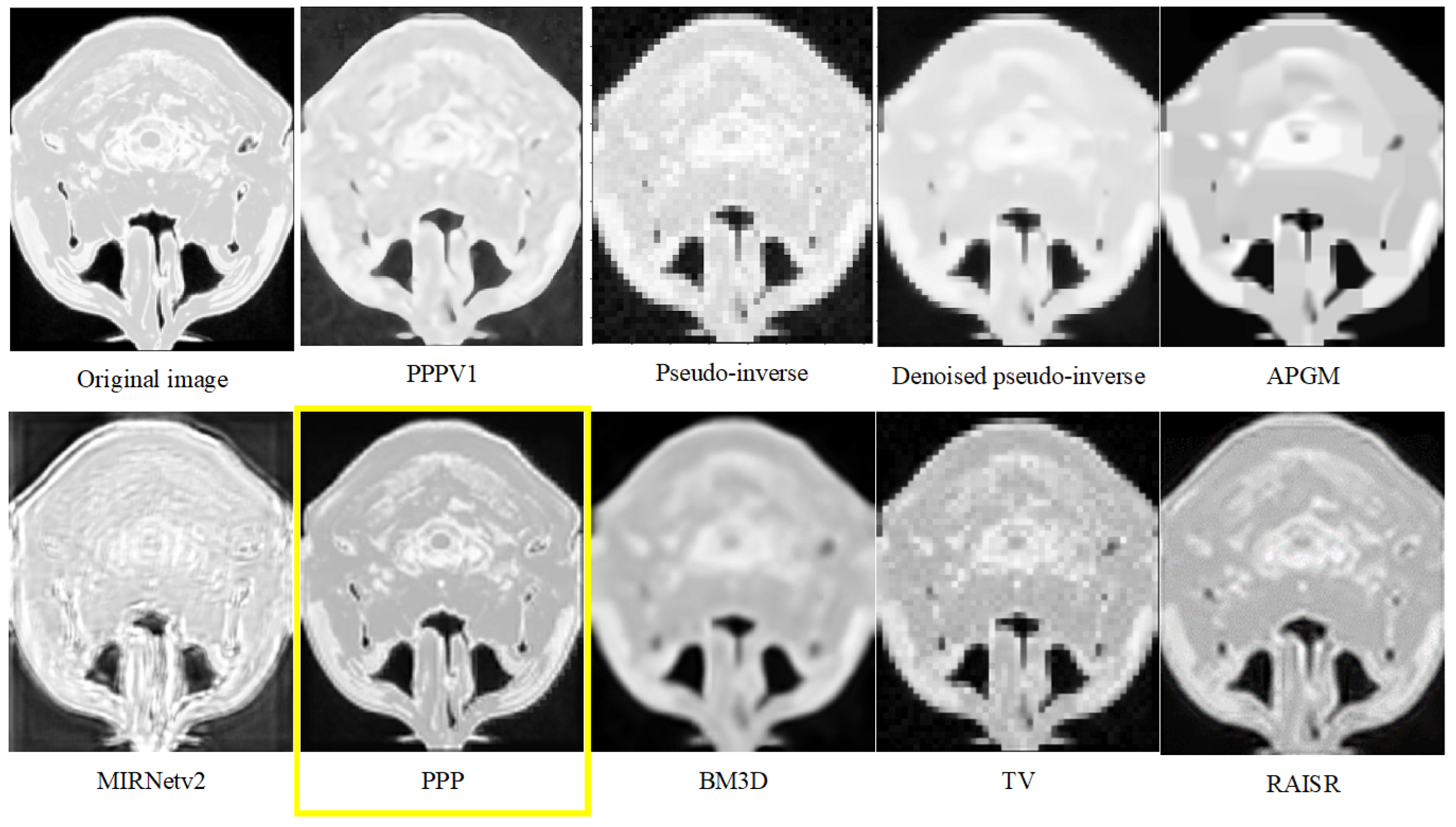
Figure 2.
Result of image 261 from Dataset 2
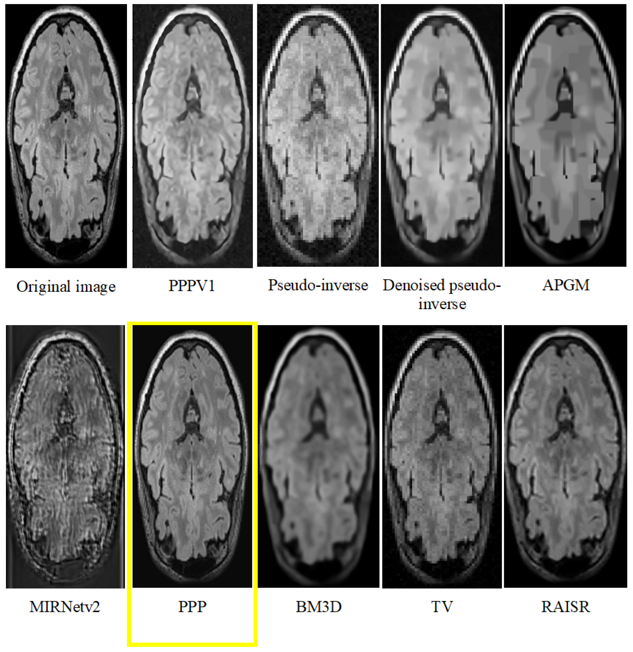
Figure 3.
Scatter plot representation and the Wilcoxon signed-rank test results of the comparison for each of the six super-resolution methods (PPP V1, Pseudo-inverse, Denoised Pseudoinverse, APGM, BM3D and TV) with the PPP method regarding PSNR values. Four stars (****) are less commonly used than one, two, or three asterisks in standard practice. If used, they might denote an extremely high level of significance, possibly at the 0.0001 level (p-value < 0.0001), while in this case all results were p=0.000, indicating an ultimately significant correlation.
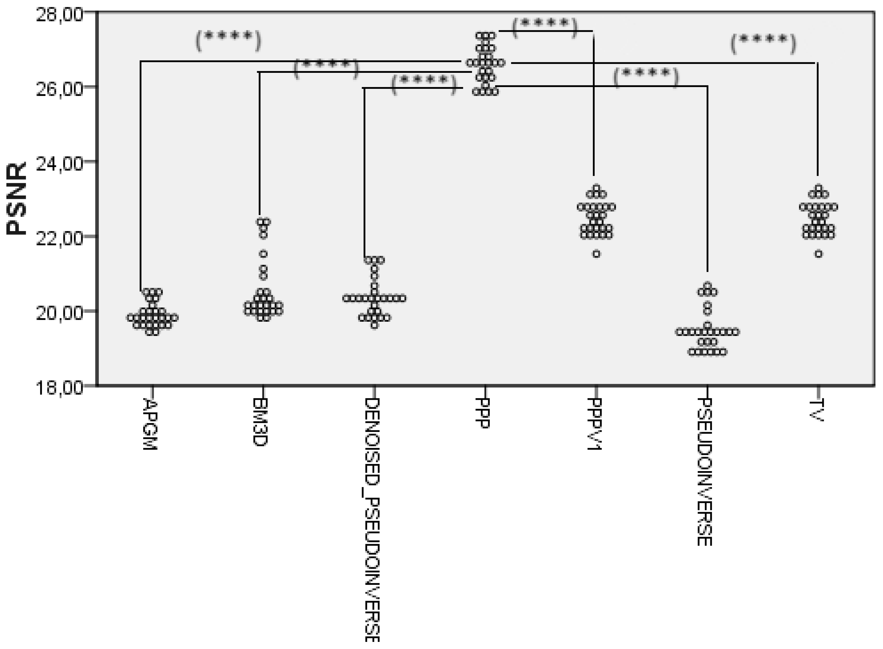

Table 1.
PSNR statistics for the two datasets of all the methods
| Dataset 1 | Dataset 2 | |||
|---|---|---|---|---|
| Average | St.Dev | Average | St.Dev | |
| PPPV1 | 22.49 | 0.44 | 25.26 | 0.25 |
| PPP | 26.59 | 0.49 | 25.67 | 0.65 |
| Pseudo-inverse | 19.52 | 0.56 | 22.81 | 0.26 |
| Denoised pseudo-inverse | 20.36 | 0.51 | 23.73 | 0.28 |
| APGM | 19.91 | 0.34 | 23.78 | 0.22 |
| BM3D | 20.58 | 0.82 | 23.72 | 0.36 |
| TV | 22.48 | 0.44 | 23.50 | 0.29 |
| RAISR | 21.99 | 0.43 | 25.77 | 0.32 |
| MIRNetv2 | 14.05 | 0.27 | 14.26 | 0.18 |
Table 2.
NIQE statistics for the two datasets of all the methods
| Dataset 1 | Dataset 2 | |||
|---|---|---|---|---|
| Average | St.Dev | Average | St.Dev | |
| PPPV1 | 6.14 | 0.15 | 6.66 | 0.17 |
| PPP | 5.82 | 0.15 | 6.39 | 0.16 |
| Pseudo-inverse | 14.13 | 0.36 | 14.08 | 0.35 |
| Denoised pseudo-inverse | 14.13 | 0.36 | 14.08 | 0.35 |
| APGM | 13.86 | 0.35 | 13.03 | 0.33 |
| BM3D | 10.66 | 0.27 | 11.92 | 0.30 |
| TV | 12.22 | 0.31 | 12.82 | 0.32 |
| RAISR | 5.87 | 0.15 | 9.61 | 0.24 |
| MIRNetv2 | 7.18 | 0.18 | 7.95 | 0.20 |
Disclaimer/Publisher’s Note: The statements, opinions and data contained in all publications are solely those of the individual author(s) and contributor(s) and not of MDPI and/or the editor(s). MDPI and/or the editor(s) disclaim responsibility for any injury to people or property resulting from any ideas, methods, instructions or products referred to in the content. |
© 2024 by the authors. Licensee MDPI, Basel, Switzerland. This article is an open access article distributed under the terms and conditions of the Creative Commons Attribution (CC BY) license (https://creativecommons.org/licenses/by/4.0/).
Copyright: This open access article is published under a Creative Commons CC BY 4.0 license, which permit the free download, distribution, and reuse, provided that the author and preprint are cited in any reuse.


