Submitted:
02 October 2024
Posted:
02 October 2024
You are already at the latest version
Abstract
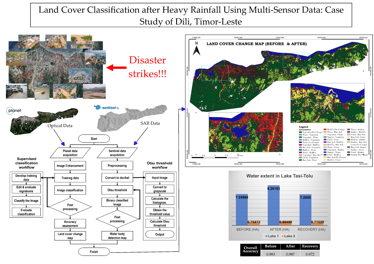
This study utilizes a combination of optical PlanetScope imagery and Synthetic Aperture Radar (SAR) data from Sentinel-1 to investigate land cover changes in Dili, Timor-Leste, following Tropical Cyclone Seroja. The primary objective is to evaluate how integrating these datasets enhances disaster monitoring and response in flood-affected areas. The Random Forest classifier, known for its robustness in handling high-dimensional and noisy data, was applied to classify land cover into six distinct classes: vegetation, water, built-up areas, bare soil, clouds, and shadows. The classification was performed across three phases—pre-disaster, post-disaster, and recovery—using Google Earth Engine (GEE). Binary segmentation using Otsu thresholding was applied to the SAR images to refine the classification by delineating water bodies from non-water areas. The study achieved high classification accuracy, with overall accuracy ranging from 97.2% to 98.7%, and the Kappa index, which measures agreement between classified and reference data, remained consistently strong, indicating reliable model performance. Key results include a significant increase in water bodies and extensive damage to vegetation and built-up areas during the post-disaster phase, followed by partial recovery in the subsequent period. Despite the high accuracy, urban areas posed classification challenges due to misclassification between built-up and bare soil categories. This research offers a methodological framework for integrating optical and SAR data with machine learning for land cover change detection in post-disaster scenarios. The societal benefits of this study include improved disaster preparedness, enhanced recovery planning, and valuable insights into flood impact mitigation in regions like Timor-Leste, where technical and data limitations persist.
Keywords:
land cover change
; change detection
; disaster monitoring
; Random Forest classifier
; Otsu Thresholding
; SAR data
; optical imagery
; Timor-Leste
1. Introduction
Timor-Leste, a Southeast Asian nation, is highly vulnerable to extreme weather due to its tropical climate and rugged mountainous terrain [1]. The recent Tropical Cyclone Seroja, which struck the country in April 2021, caused widespread devastation, resulting in significant loss of life, damage to infrastructure, and disruption of essential services such as roads and bridges. The recovery cost is estimated to exceed $420 million, underscoring the urgent need for improved disaster preparedness and response strategies [2]. Mapping and analyzing land cover changes after events like Tropical Cyclone Seroja is critical for understanding the extent of environmental damage and enhancing future resilience [3,4].
Remote sensing and Geographic Information Systems (GIS) provide essential tools for monitoring land cover changes, particularly in post-disaster scenarios, by enabling rapid and large-scale assessments [5]. The combination of optical and synthetic aperture radar (SAR) satellite data offers a comprehensive solution for overcoming challenges such as cloud cover, which limits optical imagery. SAR data from Sentinel-1 enables continuous monitoring even under adverse weather conditions, while optical data from PlanetScope, with its high spatial resolution, aids in identifying and classifying specific land cover types, such as vegetation, water bodies, and built-up areas [6,7,8].
This study leverages remote sensing and GIS technologies to detect and analyze land cover changes in Dili, Timor-Leste, following the impact of Tropical Cyclone Seroja. The primary aim is to assess how combining optical and SAR satellite data can enhance disaster response by providing more accurate insights into flood-affected areas. As disaster monitoring through remote sensing continues to evolve, it is crucial to address persistent challenges in developing countries like Timor-Leste, where access to high-resolution satellite data, sufficient training data, and technical capacity are often limited. Improving access to high-resolution satellite data, building sufficient training datasets, and increasing technical capacity can significantly enhance disaster risk reduction and recovery planning.
This research aims to address critical questions, including: (1) How can satellite imagery detect changes in land cover during and after a disaster? (2) What are the specific data requirements for accurate land cover change detection in Timor-Leste? (3) How can training data and technical knowledge gaps be mitigated to improve disaster response?
Specifically, the research aims to (1) Visualize changes in water bodies using Sentinel-1 SAR images, (2) Extract changes in land cover classes using satellite data, (3) Identify which land cover classes show significant changes during disaster events based on optical image data, (4) Perform accurate land cover classification using Google Earth Engine (GEE), and (5) Generate land cover maps for pre-disaster, post-disaster, and recovery phases.
This study is significant because it offers a methodological framework for using remote sensing and GIS in disaster response. It provides crucial insights into the specific impacts of flooding and landslides on land cover in Timor-Leste, findings that are of great interest to the fields of disaster management and environmental science, as they can inform future disaster mitigation strategies.
2. Materials and Methods
2.1. Dataset and Study Area
2.1.1. PlanetScope Dataset
This research utilizes two primary datasets: Planet Scope optical imagery and Sentinel-1 Synthetic Aperture Radar (SAR) data. Additional GIS data, such as contour lines, streets, amenities, and administrative boundaries, were also employed. The Coordinate Reference System (CRS) used for this study is EPSG:32751 - WGS 84 / UTM zone 51S. Planet Scope Ortho Tile Products, which are radiometrically and sensor corrected, orthorectified, and projected to UTM, were used. The imagery consists of three temporal stages: pre-disaster, post-disaster, and recovery. It covers an area of 24.6 x 16.4 km, with a spatial resolution of 3 x 3 meters and a daily temporal resolution.

Table 1.
Characteristics of the PlanetScope Imagery used in this research.
| Period | Product name | Acquisition Date (yyyy/mm/dd) |
Spatial Resolution |
|---|---|---|---|
| Pre-disaster | 4233514_5135126_2021-03-06_2403_BGRN_SR | 2021/03/24 | 3 m |
| Post-disaster | 4355850_5135126_2021-04-09_2403_BGRN_SR | 2021/04/09 | 3 m |
| Recovery | 4598466_5135126_2021-06-18_2403_BGRN_SR | 2021/06/18 | 3 m |
2.1.2. Sentinel-1 SAR Dataset
Sentinel-1 SAR data is used for water body extraction. The Sentinel-1 satellites provide data with an Interferometric Wide swath mode, double polarization (VV+VH), a swath width of 250 km, and a resolution of 5-20 meters.
Table 2.
Characteristics of the Sentinel-1 SAR Imagery used in this research.
| Period | Product name | Acquisition Date (yyyy/mm/dd) |
Flight Direction |
|---|---|---|---|
| Pre-disaster | S1A_IW_GRDH_1SDV_20210312T100017_20210312T100046_036963_045954_F893 | 2021/03/12 | Descending |
| Post-disaster | S1A_IW_GRDH_1SDV_20210405T100018_20210405T100047_037313_046573_0CA0 | 2021/04/05 | Descending |
| Recovery | S1A_IW_GRDH_1SDV_20210604T100021_20210604T100050_038188_0481CD_6A38 | 2021/06/04 | Descending |
2.1.3. Study Area
This study was conducted in Timor-Leste, specifically focusing on its capital city, Dili, located between 8°34′S latitude and 125°34′E longitude. Timor-Leste, officially known as the Democratic Republic of Timor-Leste, is an island nation covering approximately 14,874 km². The climate of Timor-Leste is greatly influenced by the El Niño Southern Oscillation (ENSO), which can modify the timing of the annual rainfall peak and vary the total quantity of rainfall by up to 50% throughout the year[1].
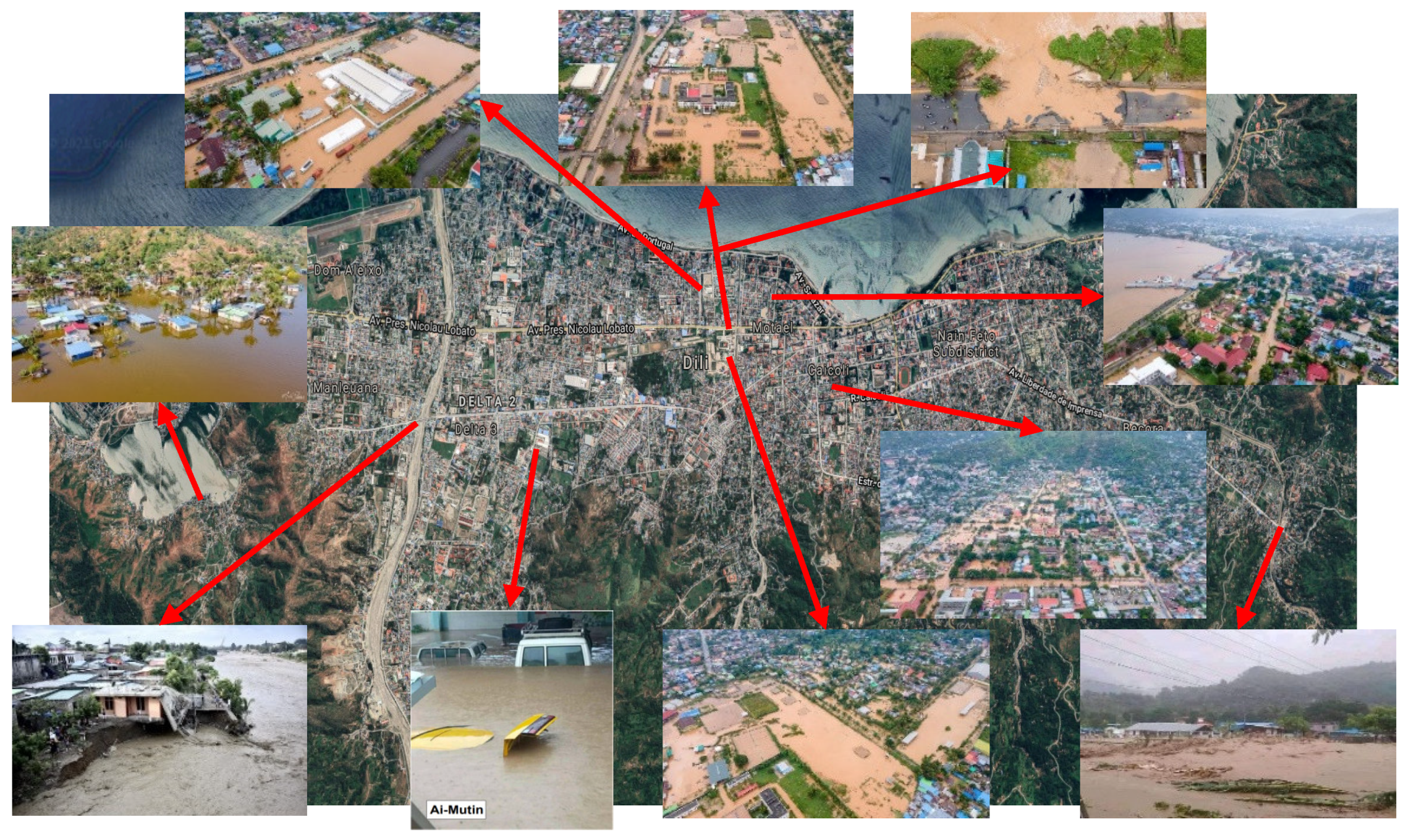
The 24-hour rainfall on April 4, 2021, was almost ten times higher than on any other day during the rainy season, with an average intensity of over 14 millimeters per hour and a peak intensity of over 70 millimeters per hour. The rain gauge at Dili’s International Airport recorded a staggering 341.8 millimeters of precipitation in just 24 hours. This extreme rainfall caused significant damage through secondary hazards in the form of flash floods, landslides, and liquefaction, as shown in Figure 2 which were exacerbated by the country’s natural topography [9]. Dili city experiencing rapid population growth and urbanization. This, coupled with inadequate drainage systems and large rivers, exacerbates the city’s susceptibility to flooding. Dili’s terrain, with its complex mix of surrounding mountains and a smaller lowland region, presents a significant challenge in managing floods.
Figure 1.
Study Area map showing the most affected city during the disaster.
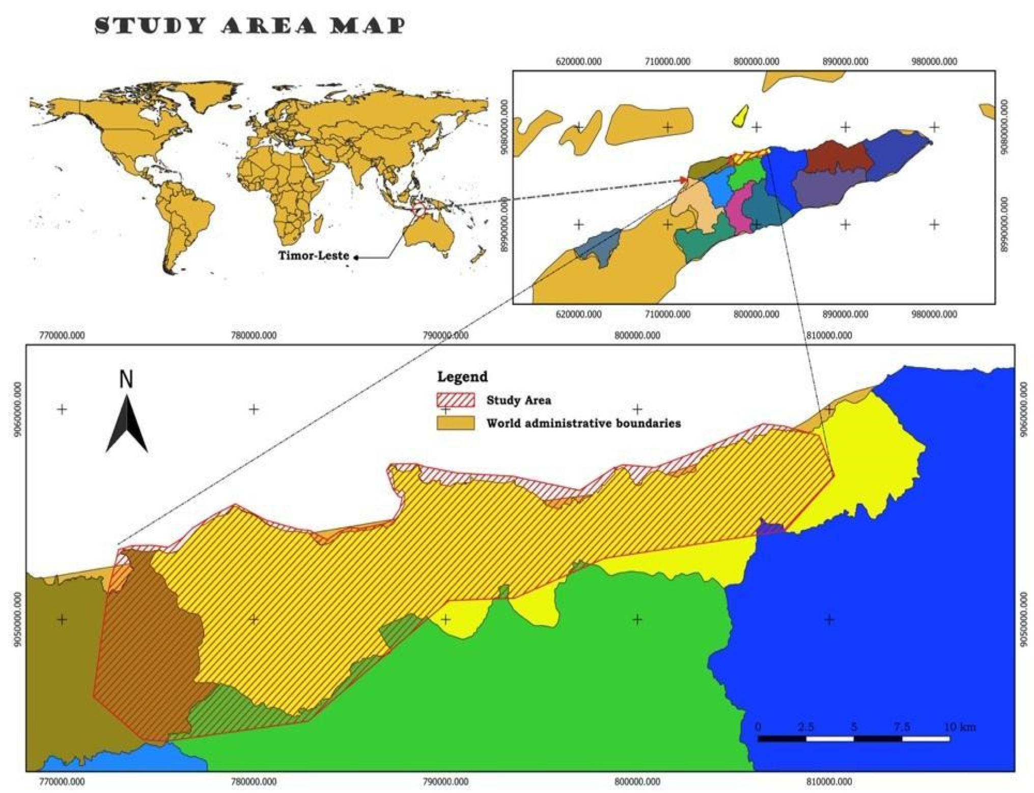
Figure 2.
Flood Impact in Dili, Timor-Leste: Aerial and Ground-Level Visual Documentation.
2.2. Methodologies
The method proposed for detecting land cover change and delineating flood extents integrates both Sentinel-1 SAR data and PlanetScope optical data, as illustrated in Figure 3. This process involves the following key steps: (a) Access a series of Sentinel-1 SAR Ground Range Detected (GRD) images and PlanetScope optical imagery covering the pre-disaster, post-disaster, and recovery phases (e.g., one week before and after the flood event) through Google Earth Engine (GEE). Preprocessing steps such as speckle filtering (to reduce noise), orthorectification (to correct geometric distortions), and calibration (to adjust for sensor inconsistencies) are applied to the SAR data to enhance water area identification [10]. (b) Perform automatic segmentation using thresholding on the SAR images to distinguish water bodies from non-water areas. The Otsu thresholding method is applied to create binary images that represent water and non-water regions [11,12]. (c) Enhance the initial classifications using supervised classification techniques in PlanetScope data, supported by fuzzy logic to improve the delineation between land cover classes, such as vegetation, built-up areas, and water bodies, by handling the uncertainty in classification boundaries. (d) Post-process the classified images using morphological operations such as erosion and dilation to refine the flood maps. The accuracy of the results is validated by comparing the binary water masks derived from SAR data with reference water masks created from high-resolution PlanetScope optical images, ensuring the robustness of the final flood extent maps.
2.2.1. Image Enhancement and Training Data Develpment
To enhance the imagery, we utilize both true-color and false-color band combinations. The true-color band combination (Red, Green, Blue) provides a natural representation of the land surface as seen by the human eye, while the false-color band combination (which assigns near-infrared, red, and green bands to visible colors) is effective for highlighting vegetation health and water bodies. These band combinations allow for improved interpretation of the data. Figure 4, depicting both true-color and false-color band combinations, should be placed here to illustrate the visual differences and benefits of each method.
The training dataset is constructed by manually selecting regions of interest (ROIs) within the PlanetScope imagery, representing distinct land cover types (e.g., water, vegetation, and built-up areas), as shown in Figure 5. These ROIs provide the spectral signatures used to train the classification algorithm to identify similar land cover types throughout the image (reference needed). The data is split into two subsets, with 80% used for training and 20% reserved for validation. This split reduces the risk of overfitting and ensures reliable classification performance.
In this supervised classification approach, training data is collected by delineating areas representing different land cover types using polygons in Google Earth Engine (GEE). The spectral reflectance properties of materials like water, bare ground, and vegetation form the basis for classification. The algorithm uses the mean spectral signatures from the training sites to classify unlabelled pixels in the imagery, assigning each pixel to the most similar land cover class. Several important considerations must be taken into account during the creation of training data, as outlined below:
- General Rule: For n bands of data, it is necessary to collect more than 10n pixels of training data for each class (e.g., for a 5-band dataset, collect more than 50 pixels per class).
- Size: The training site must be large enough to represent the class accurately while including some variability within the class. It should also include some pixels that do not strictly belong to the class to account for natural variability and borderline cases.
- Location: Training sites must be selected from various parts of the image to capture the full variability of the class, not just from one localized area.
- Number: Ideally, five to ten training sites per class are recommended, ensuring more than one site for each class.
- Uniformity: Each training site should contain relatively homogeneous pixels to ensure consistency, but should also capture class variability without being excessively heterogeneous.
2.2.2. Random Forest Supervised Classification
The core of the land cover classification is performed using the Random Forest algorithm, a robust machine learning method known for its ability to handle high-dimensional and noisy data. The algorithm constructs multiple decision trees from the training data, where each tree makes a prediction. This ensemble approach helps reduce overfitting and improves model generalization [13,14]. The final classification is determined by majority voting across all trees in the forest. The Random Forest algorithm is applied using Google Earth Engine’s ee.Classifier.smileRandomForest. For this study, 500 decision trees are used in the training process, striking a balance between model accuracy and computational efficiency.
The classification is based on six predefined land cover classes: Vegetation (0), Water (1), Built-up (2), Bare soil (3), Cloud (4), and Shadow (5). These predefined classes ensure consistency in the naming and labeling of the training data, which is essential for replicability and accuracy. This standardized classification scheme is crucial for maintaining accuracy and reliability across the dataset.
2.2.3. Morphological Operation and Accuracy Assessment
These operations, including erosion (to remove small, isolated misclassifications) and dilation (to enhance connected regions), are applied to refine the classified images by reducing classification noise and eliminating small misclassified regions [15,16,17], particularly around the boundaries of water bodies and built-up areas.
The classification is validated through an accuracy assessment, where a confusion matrix is generated to compare the classified land cover with the actual land cover, as indicated by ground-truth data collected from field surveys or high-resolution imagery. Metrics such as overall accuracy (the percentage of correctly classified pixels), user accuracy (the reliability of the classification for each class), producer accuracy (the probability that a certain class is correctly represented), and Kappa statistics (a measure of agreement between the classification and ground-truth data) are calculated to ensure the reliability of the classification.
Overall Accuracy measures the proportion of correctly classified instances (both true positives and true negatives) out of the total number of instances in the dataset, providing a general indication of the classification’s performance [18].
Overall Accuracy (OA) is calculated using the formula:
where TP is the number of true positives, TN is the number of true negatives, FP is the number of false positives, and FN is the number of false negatives.
Producer’s Accuracy measures the percentage of correctly classified pixels for a particular class, relative to all the pixels that truly belong to that class (actual positives). This metric is important because it reflects how well the classification model identifies the actual occurrences of a given class [18].
Producer’s Accuracy is calculated using the formula:
where TP is the number of true positives (correctly classified pixels), and FN is the number of false negatives (pixels that were not classified as belonging to the class but actually do).
User’s Accuracy, also known as Precision, measures the proportion of correctly classified pixels for a given class, relative to all pixels that were classified as belonging to that class. This metric is important because it reflects how accurate the classification is for the predicted class [18].
User’s Accuracy (UA) is calculated using the formula:
where TP is the number of true positives (correctly classified pixels), and FP is the number of false positives (pixels that were incorrectly classified as belonging to the class but actually belong to a different class).
The Kappa Coefficient is a statistical measure of inter-rater agreement or classification accuracy that accounts for chance agreement [8]. The Kappa statistic ranges from -1 to 1, with 1 indicating perfect agreement, 0 indicating chance-level agreement, and negative values showing disagreement worse than random chance. It is particularly useful for evaluating classification models, as it provides a more robust measure than overall accuracy, especially in situations where class imbalances may make overall accuracy misleading.
The Kappa Coefficient (k) is calculated using the formula:
Where
- Po is the observed accuracy, which is the overall accuracy of the classification model.
- Pe is the expected accuracy due to chance, calculated as:Here:
- N is the total number of samples,
- is the sum of values in row iii of the confusion matrix,
- is the sum of values in column iii of the confusion matrix,
- and is the total number of classes.
In GEE, Overall Accuracy represents the percentage of correctly classified pixels across all land cover types, providing a broad measure of the model’s overall performance. User’s Accuracy measures the proportion of correctly classified pixels for each class, indicating how reliable the classification is for a given land cover type. Producer’s Accuracy assesses how well the model captures or identifies each land cover class, reflecting the completeness of the classification for each class. The Kappa Coefficient adjusts for the possibility of chance agreement, providing a more refined measure of classification accuracy, with values closer to 1 indicating strong agreement.
These metrics are calculated in GEE [18] using confusionMatrix functions: Accuracy() for Overall Accuracy, consumersAccuracy() for User’s Accuracy, producersAccuracy() for Producer’s Accuracy, and kappa() for the Kappa Coefficient.
2.2.4. Binary Segmentation with Otsu Thesholding
Otsu thresholding is a widely used image segmentation technique, particularly effective for distinguishing objects of interest, such as water bodies, from the background in grayscale images [19]. In this study, Sentinel-1 SAR imagery is processed using Python libraries like rasterIO, OpenCV, NumPy, and Matplotlib. The Otsu method automatically determines the optimal threshold based on the histogram of pixel intensities, segmenting the image into water and non-water areas [19]. The result is a binary image where water bodies are represented by pixel values of 1, and other areas by 0.
The segmentation process begins with preprocessing Sentinel-1 images using the European Space Agency’s (ESA) SNAP software. SNAP ensures that the data is radiometrically and geometrically corrected, applying necessary operations such as orbit correction, calibration, and terrain correction to prepare the SAR data for accurate analysis. Once preprocessed in SNAP, the images are converted to the decibel (dB) scale to enhance the visibility of radar backscatter differences. Otsu’s method is then applied to perform binary segmentation, simplifying the classification of water bodies for further analysis. The segmented images are exported in GeoTIFF format, preserving georeferencing information. These binary images are then imported into QGIS, where they are converted into vector files for precise waterline delineation.
3. Results
3.1. Land Cover Map
The land cover classification, performed using the Random Forest algorithm in Google Earth Engine (GEE), which was selected for its ability to handle high-dimensional data and provide accurate results, produced three key maps: pre-disaster, post-disaster, and recovery phase land cover maps. These maps classified the study area into six distinct land cover types: vegetation, water, built-up areas, bare ground, clouds, and shadow. The results reveal significant changes in land cover caused by the disaster, including widespread flooding and damage to vegetation, as well as subsequent recovery efforts
Figure 6 shows the pre-disaster land cover map, establishing a baseline with extensive areas of vegetation and built-up zones. Figure 7, the post-disaster map, highlights the extent of damage, with a notable increase in water bodies due to flooding, and a reduction in vegetation and built-up areas. The final map, Figure 8, illustrates the recovery phase, showing the partial restoration of vegetation and urban areas, with a noticeable regrowth of plant life and rebuilding in certain regions, while some areas remain affected by bare ground or prolonged flooding.
3.2. Accuracy Assessment Results
Table 3, Table 4 and Table 5 provide confusion matrices for the pre-disaster, post-disaster, and recovery periods. In the pre-disaster phase, vegetation dominates the classification, with 4,084 correctly classified pixels out of 4,085 total pixels, reflecting the large proportion of vegetated land in the study area before the disaster. Post-disaster, a similar pattern is observed, though a slight increase in misclassification is evident, particularly in the shadow and cloud classes. The recovery phase shows a reduction in the number of classified pixels, likely due to fewer reference data points, as the region undergoes significant changes that make it harder to collect consistent ground-truth data.
Table 6 demonstrates that overall classification accuracy remains high across all three periods, with pre-disaster accuracy at 98.3%, post-disaster accuracy at 98.7%, and recovery accuracy at 97.2%. This slight decrease in recovery accuracy suggests that land cover changes introduced some complexities in classification, though the model still performed well.
Table 7 summarizes the user’s and producer’s accuracy for each land cover class before, after, and during recovery. Vegetation consistently maintains high accuracy, with both user’s and producer’s accuracy exceeding 99%. Water is perfectly classified during the post-disaster phase (100% producer’s accuracy), while built-up areas show the lowest classification accuracy, particularly in the pre-disaster phase, with user’s accuracy at 82.1% and producer’s accuracy at 68.1%, reflecting challenges in classifying urban areas.
Table 8 presents the Kappa index values, which measure the agreement between classified and reference data. The Kappa index is 0.976 before the disaster, 0.980 post-disaster, and 0.951 during recovery, indicating strong agreement throughout the classification process. The slight decrease in the recovery phase reflects the complexities introduced by land cover changes during this period.
3.3. Land Cover Change Map
The Land Cover Change Map was generated using the Random Forest Algorithm on the Google Earth Engine (GEE) platform. The algorithm’s outputs were subsequently imported into Quantum GIS (QGIS) for change detection analysis. Two images from different time periods were used to evaluate land cover changes. The Semi-Automatic Classification Plugin in QGIS was used for preprocessing, including atmospheric correction and resampling, to ensure consistency between the images. The Land Cover Change tool was then applied to facilitate the analysis. The results of land cover changes for three distinct periods—pre-disaster, post-disaster, and recovery—are displayed in Figure 9.
In this analysis, the pre-disaster image serves as a reference for the initial classification, while the post-disaster image is used for the new classification. This approach is applied to compare changes between the pre-disaster and post-disaster phases, the post-disaster and recovery phases, and the pre-disaster and recovery phases. The comparison results are shown in Figure 10, Figure 11 and Figure 12.
In Figure 10, significant changes, indicated by light brown, are evident in the eastern part of Dili, suggesting a considerable loss of crops washed away by the river due to excessive water. Additionally, in the Lake of Tasi-Tolu, an extension of water is visible, represented by a light blue color, indicating an increase in the lake’s volume during the post-disaster phase. In contrast, Figure 11 demonstrates significant vegetation recovery during the recovery phase, represented by light green, while the lake’s water volume decreases. Figure 12 reveals that some vegetation did not fully recover, as shown by a comparison of the pre-disaster and recovery phase land cover classifications. This indicates that some vegetation and crops were fully covered by sedimentation caused by river overflow during the disaster.
3.4. Water Body Detection Map
The binarized images, where water bodies are represented by pixels with values of 1 and non-water areas by 0, are loaded into QGIS for waterline extraction and selection. Waterline selection in the vector files is done by comparing them with Google satellite imagery or other high-resolution satellite data to ensure accurate and consistent delineation. The yellow lines in Figure 13 depict the waterline of Lake Tasi-Tolu in Dili during the pre-disaster, post-disaster, and recovery phases. Figure 14 shows the statistics values of the changes in water volume across the three observation periods by extracting the area of the waterline from the classified image. Figure 15 illustrates water detection using Sentinel-1 SAR data for the three observation periods.
3.5. Correlation between SAR and Optical Results
The water detection results from land cover change detection using PlanetScope imagery and binary-segmented Sentinel-1 imagery were combined to visualize the differences between the two datasets. In Figures 16a, 16b, and 16c, blue indicates water detection in the optical (PlanetScope) imagery, while red indicates water detection in the Sentinel-1 SAR imagery.
3.6. Comparison with Preliminary Results by UNITAR and UNOSAT
Figures 17a and 17b present preliminary results from UNITAR-UNOSAT, which used Pleiades imagery to assess the aftermath of the disaster in Timor-Leste [20]. Their analysis highlighted regions most impacted by flooding, focusing on changes in land cover, such as water bodies, bare soil, and built-up areas. These early results, derived from high-resolution optical imagery, provided a visible assessment of the immediate changes caused by the disaster.
Figures 17c and 17d show the classification results from this study, capturing similar patterns of change, such as landslides and vegetation loss due to flooding. A strong correlation exists between the two analyses, as both consistently identify severely affected areas.
The Random Forest classification using PlanetScope data in this study further validates the preliminary findings, offering a more automated and scalable method for detecting land cover changes. The observed decrease in vegetation and the increase in water and bare soil confirm the reliability of this approach, aligning with established methodologies such as those used by UNITAR-UNOSAT. This consistency underscores the effectiveness of combining high-resolution satellite imagery with machine-learning algorithms for practical disaster assessment and recovery monitoring.
4. Discussion
In this paper, we derived the training data through visual interpretation of high-resolution PlanetScope satellite imagery. Generating this training data required local knowledge to ensure accurate representation, which was then used to feed the Random Forest Supervised Classification Algorithm. The classification results exhibited ‘salt-and-pepper’ noise, caused by spectral variability in the imagery, despite the high overall accuracy. We perform the morphological analyses to deal with the noise, and the results demonstrate a better corrected version of the classification results as depicted in Figure 18. Nevertheless, the overall accuracy provided a strong representation of the land cover classification results for the pre-disaster, post-disaster, and recovery phases, with accuracies of 97.6%, 98%, and 95.1%, respectively.
The role of SAR imagery in this study primarily focuses on detecting the water extent in the lake, as this location was identified as one of the inundated areas during the heavy rainfall. SAR technology is capable of detecting water regardless of weather conditions. The binary segmentation results revealed a significant change in water volume by comparing the waterline size across the three images.
5. Conclusions
In the supervised classification approach, knowledge of land cover types is essential for identifying and classifying land cover classes. Creating reference data, or training data, requires the researcher to accurately identify land cover types, as this data is used to train the algorithm. The algorithm then recognizes and categorizes pixels that are statistically similar to the training data. To ensure the classification accurately represents all predefined classes, the training data must be evenly distributed across the image to capture pixel variations.
The image classification results show that land cover types are well-classified, with an overall accuracy exceeding 90% across all three images. Once classification is completed, accuracy assessment is performed using the cloud-based platform Google Earth Engine to determine whether the classification is accurate or needs further refinement. Training data is crucial for both training the algorithm and validating the results, with 20% of the data randomly selected for validation.
In addition to optical data, Sentinel-1 SAR imagery provides valuable insights, as it can penetrate clouds and operate in all weather conditions, day or night. This makes it highly beneficial for detecting both temporary and permanent water bodies, especially in flood and wetland monitoring. The use of the Otsu thresholding binary segmentation method on SAR data is not widely researched, requiring further investigation to enhance wetland representation. However, the findings show that water bodies can be clearly identified and accurately represented using this method.
Author Contributions
Conceptualization, P.J.F. and M.N.; methodology, P.J.F. and M.N.; software, P.J.F.; validation, P.J.F. and M.N.; formal analysis, P.J.F.; investigation, P.J.F and M.N.; resources, M.N.; data curation, P.J.F.; writing—original draft preparation, P.J.F; writing—review and editing, P.J.F. and M.N.; visualization, P.J.F.; supervision, M.N. All authors have read and agreed to the published version of the manuscript.
Funding
This research received no external funding.
Data Availability Statement
Data are contained within the article.
Acknowledgments
The authors sincerely thank Planet Labs PBC (USA) for providing high-resolution PlanetScope imagery, which was essential for this study. The authors also appreciate the contributions of colleagues and institutions who offered valuable feedback and assistance throughout the research.
Conflicts of Interest
The authors declare no conflicts of interest.
References
- World Bank Group, Asian Development Bank. Climate Risk Country Profile: Timor-Leste. Washington, DC: World Bank, 2021, pp. 2-3.
- World Bank. Learning from Tropical Cyclone Seroja: Building Disaster and Climate Resilience in Timor-Leste. Washington, DC: The World Bank, December 2021, p. 6.
- Milisavljević, N., Closson, D., Holecz, F., Collivignarelli, F., Pasquali, P. “An Approach for Detecting Changes Related to Natural Disasters Using Synthetic Aperture Radar Data.” International Archives of the Photogrammetry, Remote Sensing and Spatial Information Sciences, Vol. XL-7/W3, 2015, pp. 819-826. 36th International Symposium on Remote Sensing of Environment, 11–15 May 2015, Berlin, Germany. [CrossRef]
- Mohamed, S. A., & El-Raey, M. E. “Assessment, Prediction and Future Simulation of Land Cover Dynamics using Remote Sensing and GIS Techniques.” Assiut University Bulletin for Environmental Research, Vol. 21, No. 2, October 2018, pp. 37-38.
- Parra, L. “Remote Sensing and GIS in Environmental Monitoring.” Applied Sciences, Vol. 12, 8045, 2022. [CrossRef]
- Dagne, S.S., Hirpha, H.H., Tekoye, A.T., Dessie, Y.B., & Endeshaw, A.A. “Fusion of sentinel-1 SAR and sentinel-2 MSI data for accurate Urban land use-land cover classification in Gondar City, Ethiopia.” Environmental Systems Research, 2023, Vol. 12, Article 40, pp. 1-16. [CrossRef]
- Hu, B., Xu, Y., Huang, X., Cheng, Q., Ding, Q., Bai, L., & Li, Y. “Improving Urban Land Cover Classification with Combined Use of Sentinel-2 and Sentinel-1 Imagery.” ISPRS International Journal of Geo-Information, Vol. 10, No. 8, 2021, Article 533. [CrossRef]
- Vizzari, M. “PlanetScope, Sentinel-2, and Sentinel-1 Data Integration for Object-Based Land Cover Classification in Google Earth Engine.” Remote Sensing, Vol. 14, No. 2628, 2022. [CrossRef]
- Government of Timor-Leste, United Nations, and World Bank.Post Disaster Needs Assessment: Tropical Cyclone Seroja and the Easter Flood April 2021, Executive Summary. October 2021, pp. 2-3, 6, 819.
- Filipponi, F. “Sentinel-1 GRD Preprocessing Workflow.” Proceedings, Vol. 18, 2019, Article 11. Presented at the 3rd International Electronic Conference on Remote Sensing, 22 May–5 June 2019. [CrossRef]
- Otsu, N. “A Threshold Selection Method from Gray-Level Histograms.” IEEE Transactions on Systems, Man, and Cybernetics, Vol. SMC-9, No. 1, 1979, pp. 62-66. [CrossRef]
- Günen, M.A., & Atasever, U.H. “Remote Sensing and Monitoring of Water Resources: A Comparative Study of Different Indices and Thresholding Methods.” Science of the Total Environment, Vol. 926, 2024, Article 172117. [CrossRef]
- Kulkarni, A. D., & Lowe, B. “Random Forest Algorithm for Land Cover Classification.” International Journal on Recent and Innovation Trends in Computing and Communication, Vol. 4, No. 3, 2016, pp. 58-63. https://scholarworks.uttyler.edu/compsci_fac/1​:contentReference[oaicite:0]{index=0}.
- Akar, Ö., & Güngör, O. “Classification of Multispectral Images using Random Forest Algorithm.” Journal of Geodesy and Geoinformation, Vol. 1, No. 2, 2012, pp. 105-112. [CrossRef]
- Chudasama, D., Patel, T., Joshi, S., & Prajapati, G. I. “Image Segmentation using Morphological Operations.” International Journal of Computer Applications, Vol. 117, No. 18, May 2015, pp. 16-19.
- Louverdis, G., Vardavoulia, M.I., Andreadis, I., & Tsalides, Ph. “A new approach to morphological color image processing.” Pattern Recognition, Vol. 35, 2002, pp. 1733-1741. [CrossRef]
- Priya, M.S., & Kadhar Nawaz, G.M. “Effective Morphological Image Processing Techniques and Image Reconstruction.” International Journal of Trend in Research and Development (IJTRD), Special Issue, 2017, pp. 18-22. National Conference on “Digital Transformation – Challenges and Outcomes” (ASAT in CS’17), St. Anne’s First Grade College for Women, Bangalore.
- Nicolau, A. P., Dyson, K., Saah, D., & Clinton, N. “Accuracy Assessment: Quantifying Classification Quality.” In Cloud-Based Remote Sensing with Google Earth Engine, edited by J.A. Cardille et al., pp. 135-145. Springer, 2024. [CrossRef]
- Yousefi, J. “Image Binarization using Otsu Thresholding Algorithm.” Research, May 2015. [CrossRef]
- International Disasters Charter. “Tropical Cyclone Seroja in Timor-Leste - Activation 701.” International Disasters Charter, 4 April 2021. Available online: https://disasterscharter.org/es/web/guest/activations/-/article/flood-large-in-timor-leste-activation-701- (accessed 30 September 2024).
Figure 3.
Flowchart of the study.
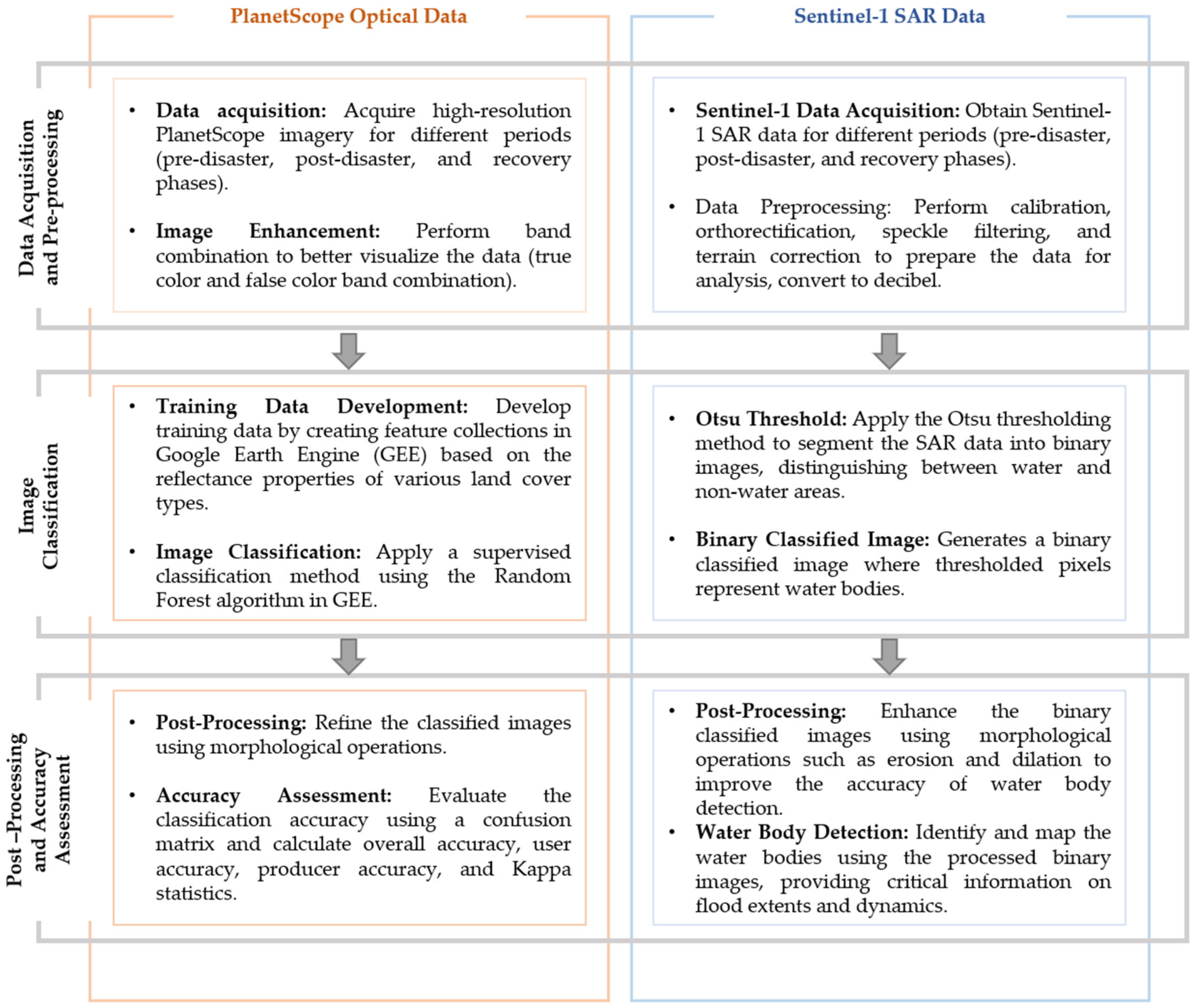
Figure 4.
True and false color band combinations: (a) True color of pre-disaster image, (b) True color of post-disaster image, (c) True color of recovery phase image, (d) False color of pre-disaster image, (e) False color of post-disaster image, (f) False color of recovery phase image.
Figure 4.
True and false color band combinations: (a) True color of pre-disaster image, (b) True color of post-disaster image, (c) True color of recovery phase image, (d) False color of pre-disaster image, (e) False color of post-disaster image, (f) False color of recovery phase image.


Figure 5.
Training data development: (a) Training data for true color image, (b) Training data for false color image.
Figure 5.
Training data development: (a) Training data for true color image, (b) Training data for false color image.
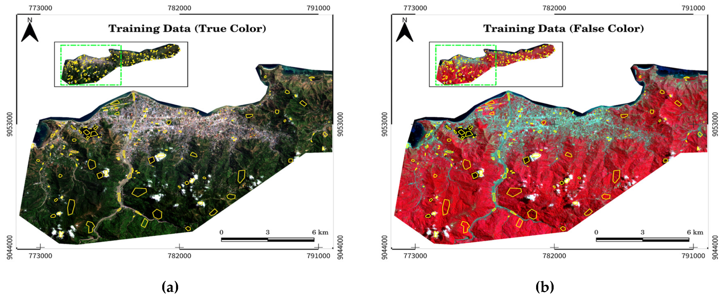
Figure 6.
Land cover map of pre-disaster.
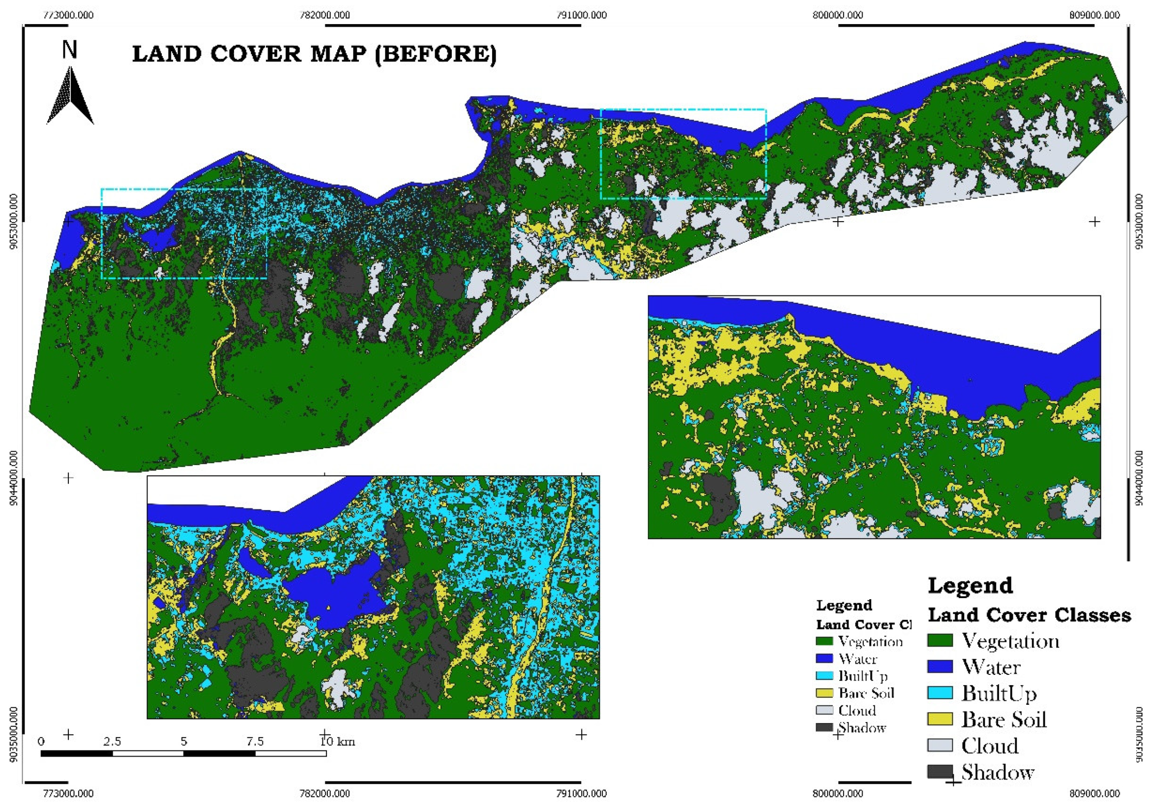
Figure 7.
Land cover map of post-disaste.
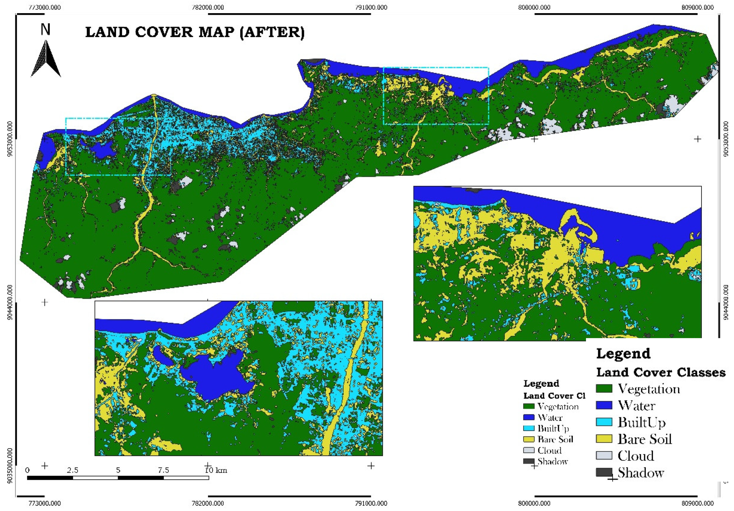
Figure 8.
Land cover map of recovery phase.
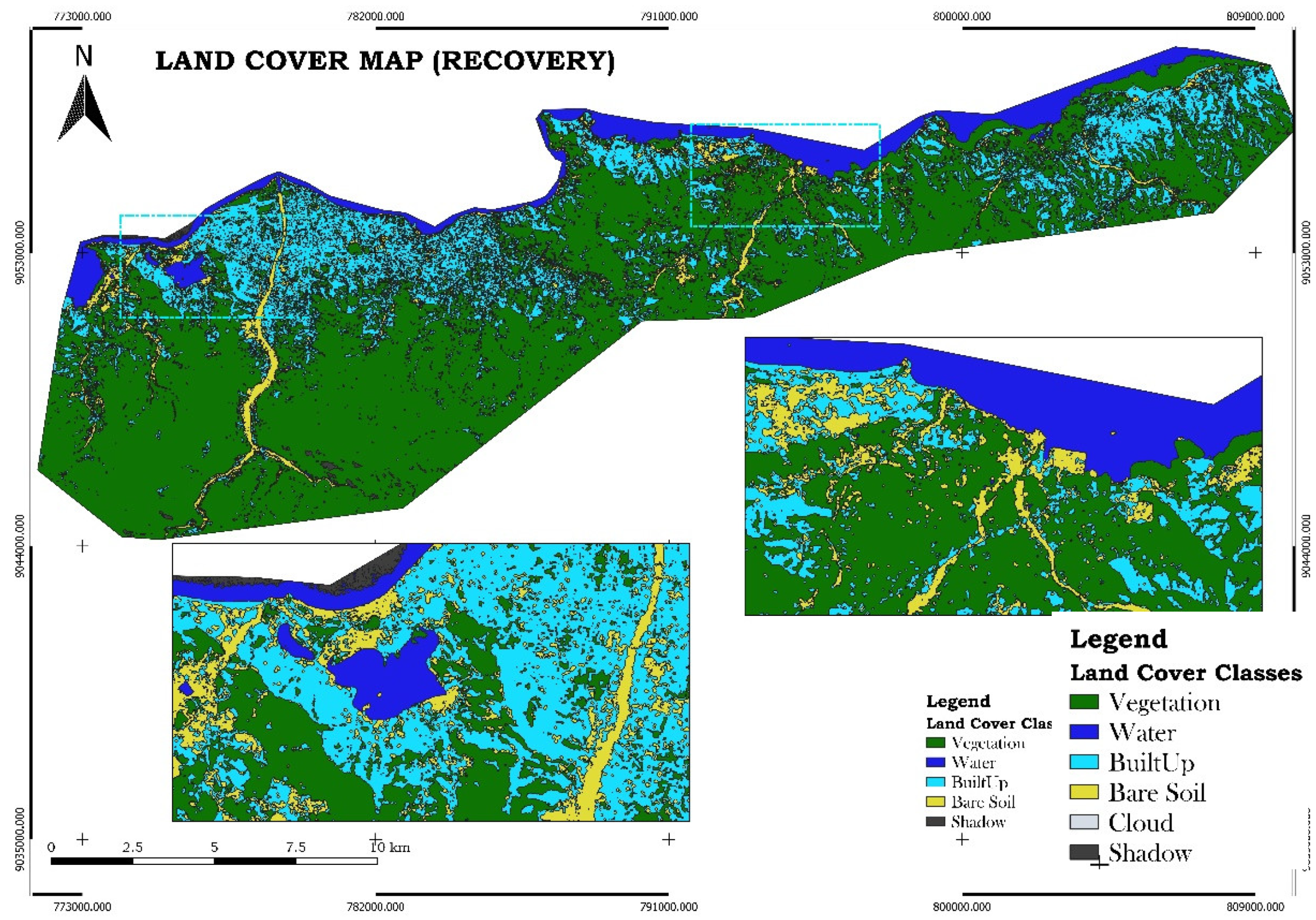
Figure 9.
Statistical values for land cover change between three different periods.
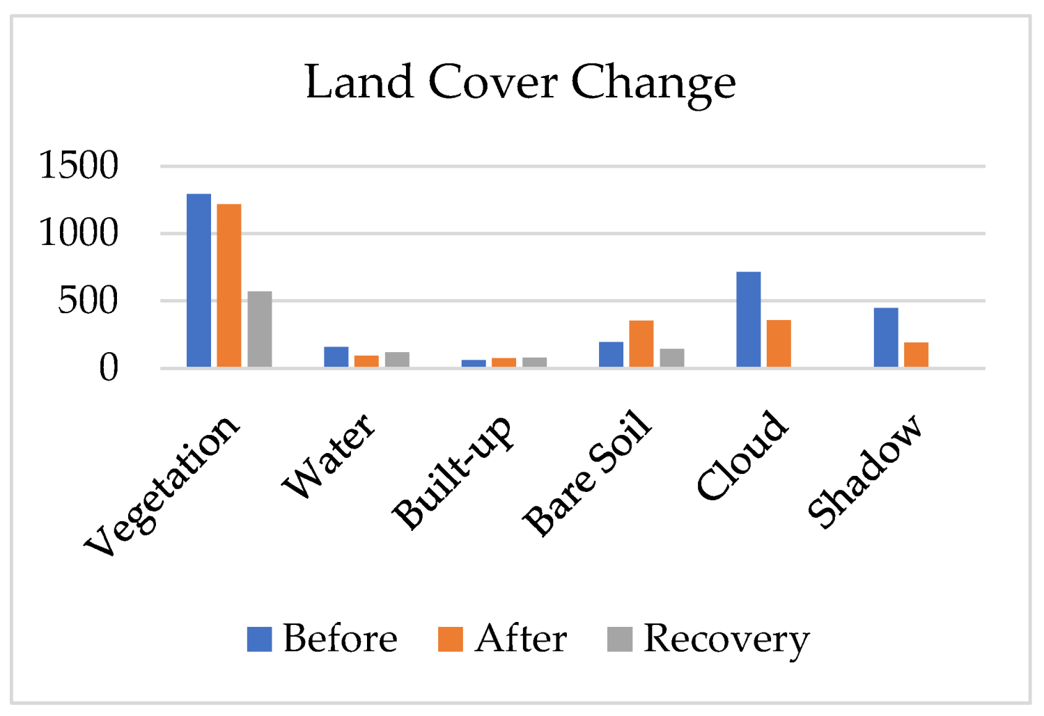
Figure 10.
Land cover change map of the pre and post disaster event.
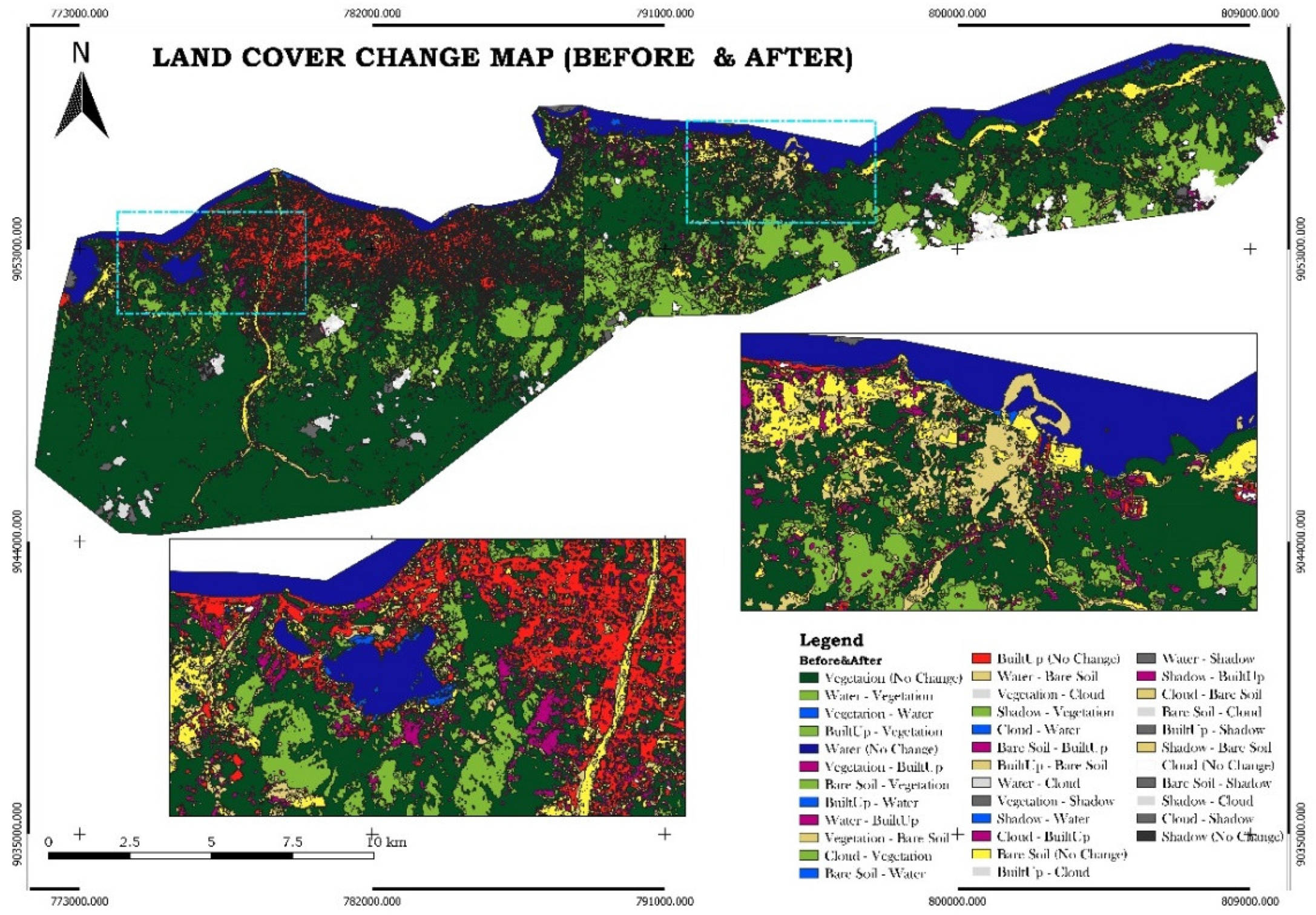
Figure 11.
Land cover change map of the post-disaster and recovery phase.
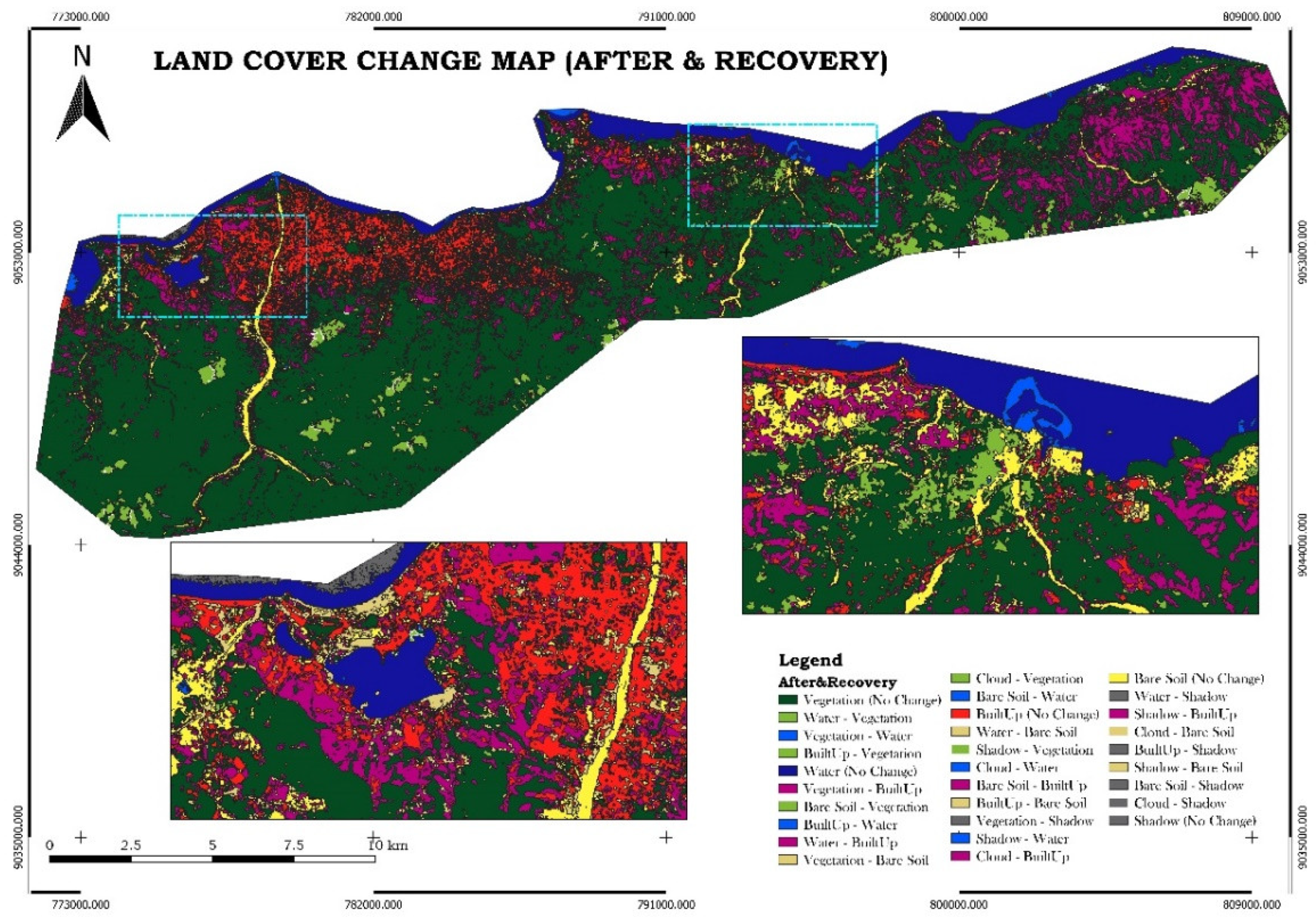
Figure 12.
Land cover change map of the pre-disaster and recovery phase.
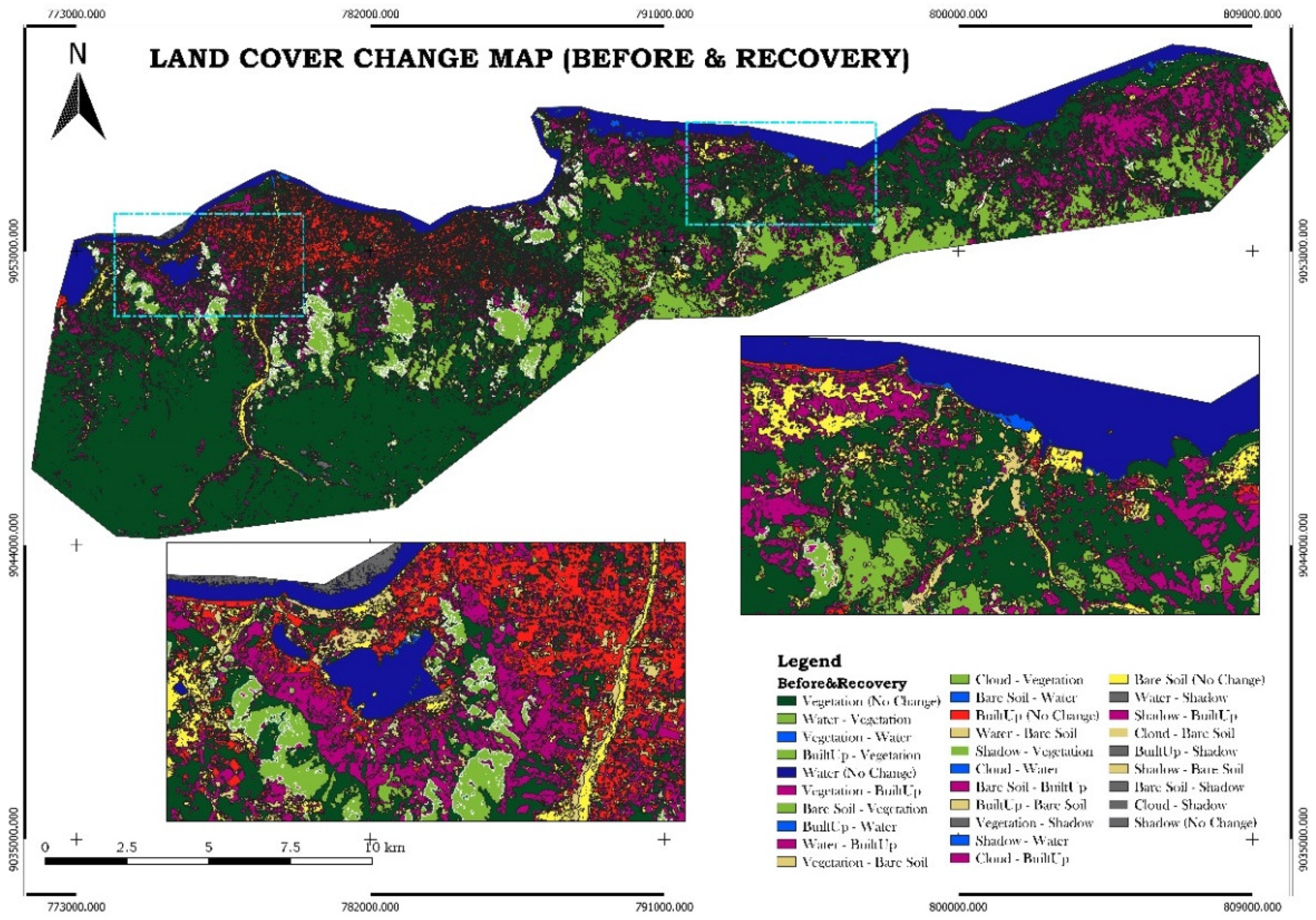
Figure 13.
Water detection in Lake Tasi-Tolu with Planet Image: (a) Water detection for pre-disaster with Planet image, (b) Water detection for post-disaster with Planet image, (c) Water detection for recovery phase with Planet image.
Figure 13.
Water detection in Lake Tasi-Tolu with Planet Image: (a) Water detection for pre-disaster with Planet image, (b) Water detection for post-disaster with Planet image, (c) Water detection for recovery phase with Planet image.
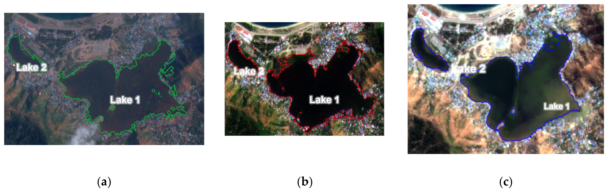
Figure 14.
Water area calculated using Planet Image classification results.
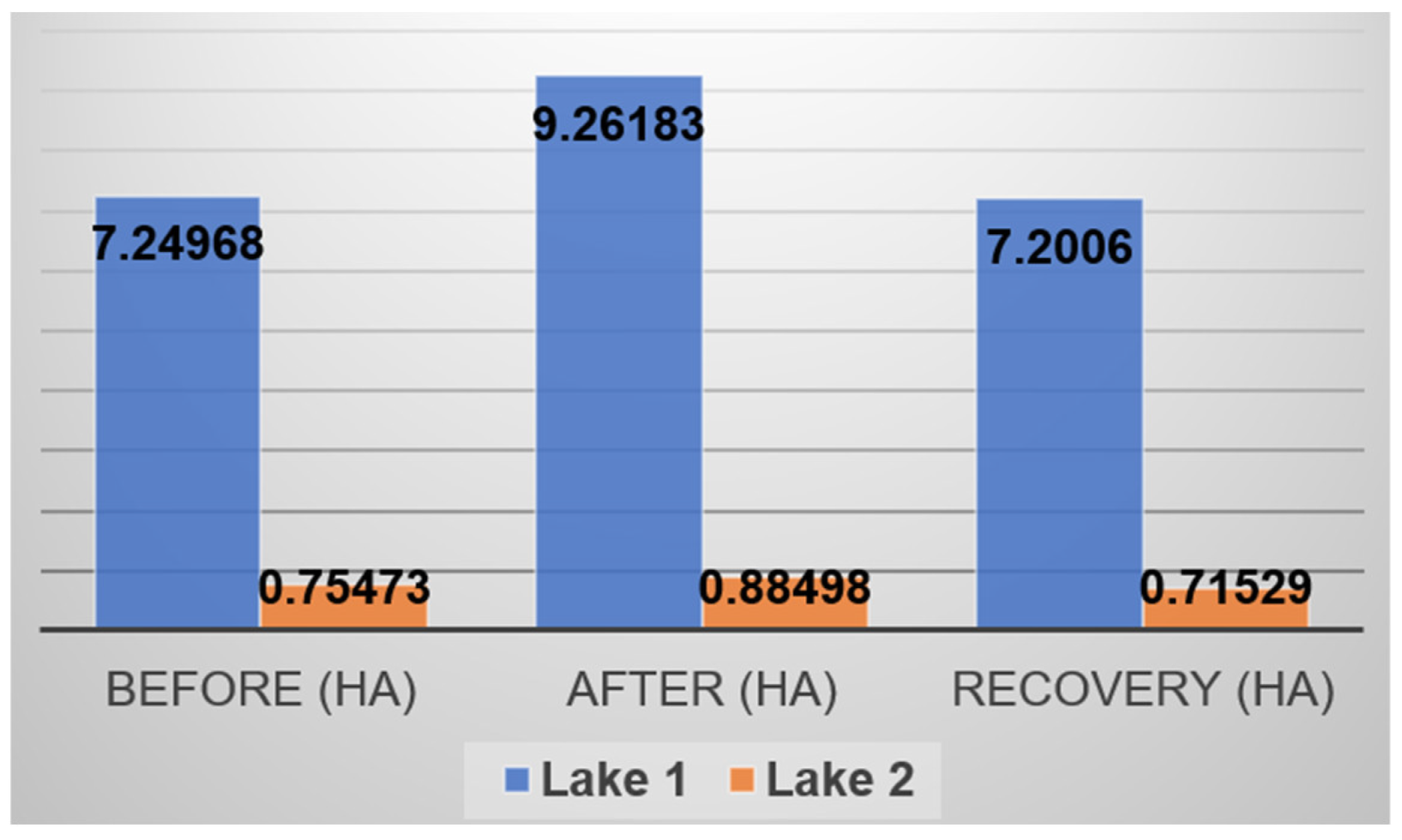
Figure 15.
Water detection in Lake Tasi-Tolu with Sentinel-1 SAR Image: (a) Water detection for pre-disaster with Sentinel-1 SAR image, (b) Water detection for post-disaster with Sentinel-1 SAR image , (c) Water detection for recovery phase with Sentinel-1 SAR image.
Figure 15.
Water detection in Lake Tasi-Tolu with Sentinel-1 SAR Image: (a) Water detection for pre-disaster with Sentinel-1 SAR image, (b) Water detection for post-disaster with Sentinel-1 SAR image , (c) Water detection for recovery phase with Sentinel-1 SAR image.
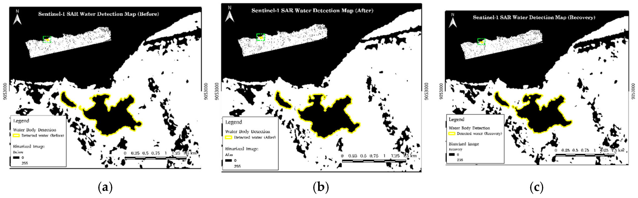
Figure 16.
Overlay of waterline detection results in Lake Tasi-Tolu using both Optical and SAR images: (a) Waterline detection for pre-disaster; (b) Waterline detection for post-disaster , (c) Waterline detection for recovery phase.
Figure 16.
Overlay of waterline detection results in Lake Tasi-Tolu using both Optical and SAR images: (a) Waterline detection for pre-disaster; (b) Waterline detection for post-disaster , (c) Waterline detection for recovery phase.
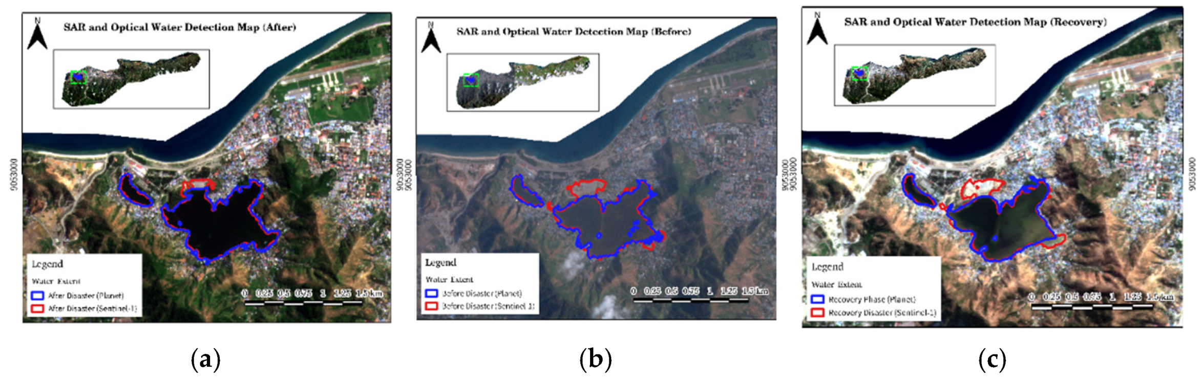
Figure 17.
Preliminary results provided by UNITAR-UNOSAT immediately after the disaster using Pleiades satellite imagery: (a) Landslide detected by Pleiades satellite, (b) Vegetation loss detected by Pleiades satellite, (c) Landslide detected by classification results, (d) Vegetation loss detected by classification results.
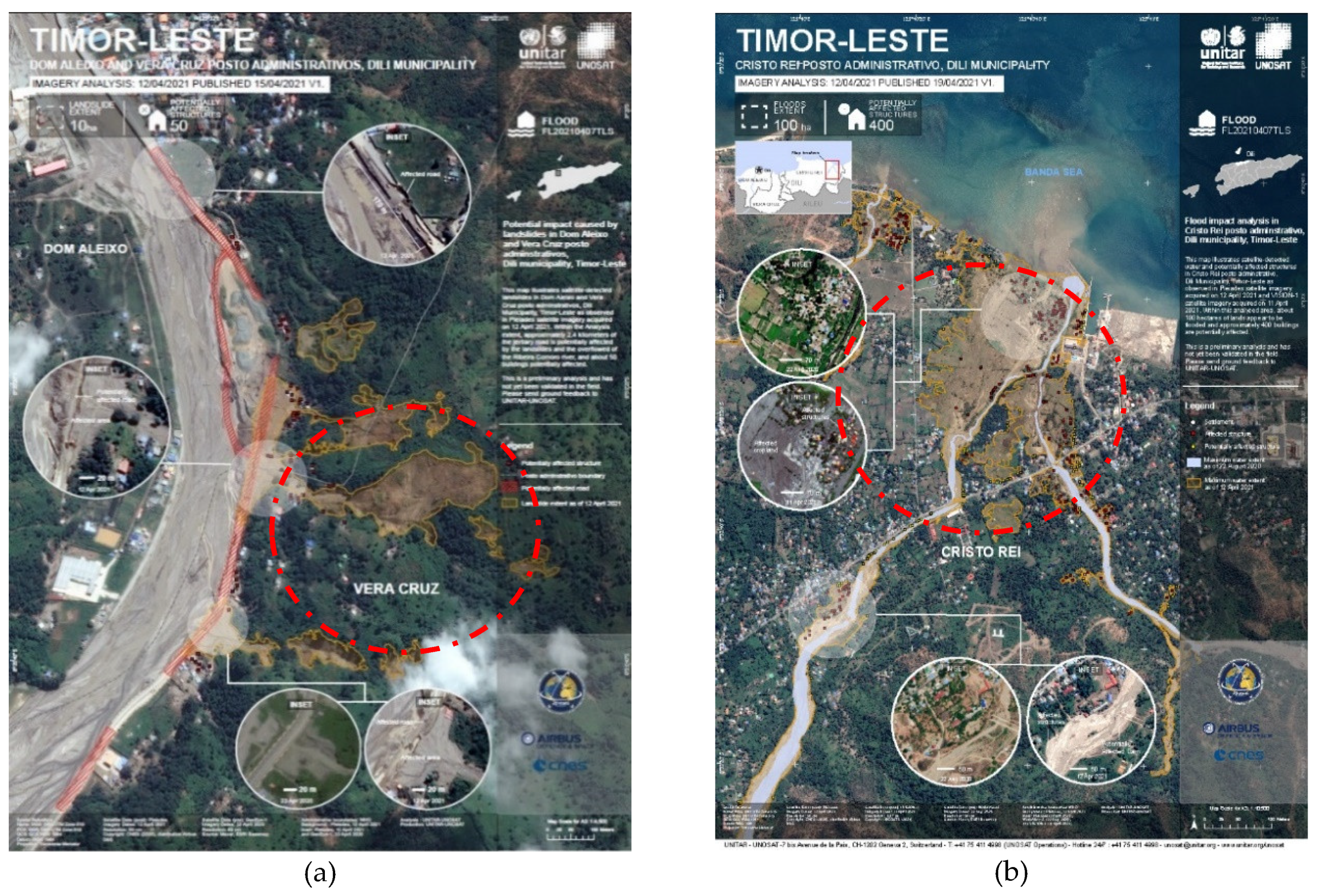
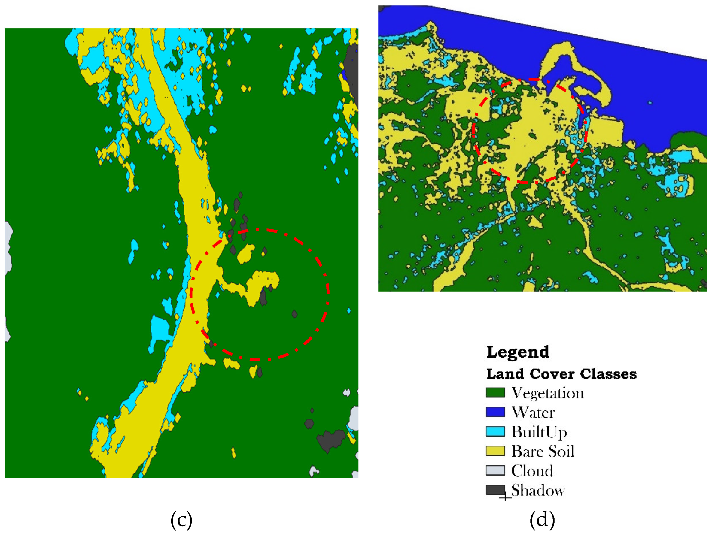
Figure 18.
Morfological operation after the classification results: (a) Noises present in the classified image ; (b) Noise corrected using the dilation approach.
Figure 18.
Morfological operation after the classification results: (a) Noises present in the classified image ; (b) Noise corrected using the dilation approach.
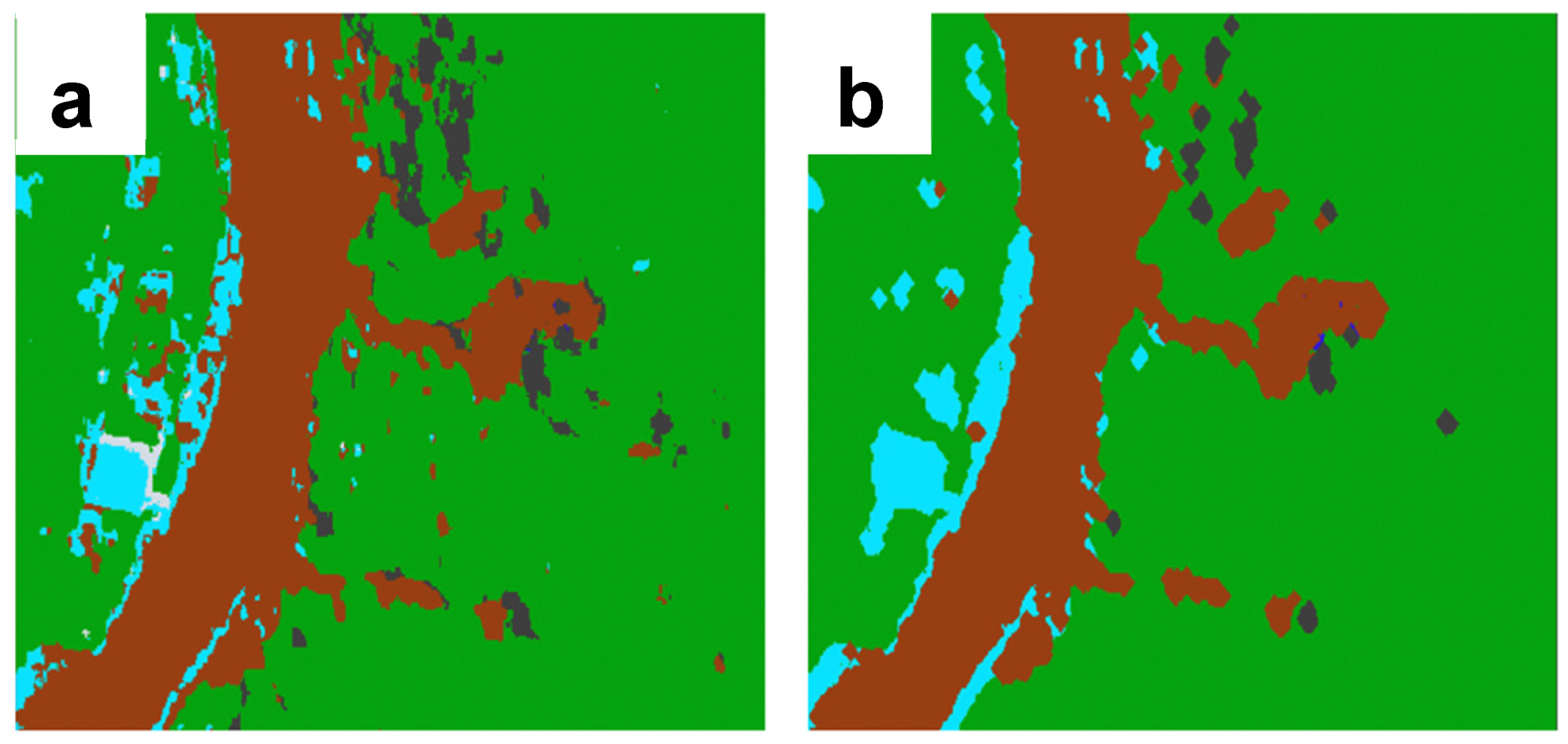
Table 3.
Confusion matrix of pre-disaster.
| Confusion matrix (Pre-disaster) | Vegetation | Water | Built-Up | Bare Soil | Cloud | Shadow | Total |
|---|---|---|---|---|---|---|---|
| Vegetation | 4084 | 0 | 0 | 0 | 0 | 1 | 4085 |
| Water | 0 | 526 | 0 | 0 | 0 | 0 | 526 |
| Built-up | 0 | 0 | 228 | 0 | 1 | 0 | 229 |
| Bare soil | 0 | 0 | 0 | 598 | 0 | 0 | 598 |
| Cloud | 0 | 0 | 0 | 0 | 2259 | 0 | 2259 |
| Shadow | 0 | 0 | 0 | 1 | 0 | 1404 | 1405 |
| Total | 4084 | 526 | 228 | 599 | 2260 | 1405 | 9102 |
Table 4.
Confusion matrix of post-disaster.
| Confusion matrix (Post-disaster) | Vegetation | Water | Built-Up | Bare Soil | Cloud | Shadow | Total |
|---|---|---|---|---|---|---|---|
| Vegetation | 3859 | 0 | 0 | 0 | 0 | 1 | 3860 |
| Water | 0 | 316 | 0 | 0 | 0 | 0 | 316 |
| Built-up | 0 | 0 | 236 | 1 | 1 | 0 | 238 |
| Bare soil | 0 | 0 | 0 | 1175 | 0 | 0 | 1175 |
| Cloud | 0 | 0 | 0 | 0 | 1085 | 0 | 1085 |
| Shadow | 2 | 0 | 0 | 0 | 0 | 577 | 579 |
| Total | 3861 | 316 | 236 | 1176 | 1086 | 578 | 7253 |
Table 5.
Confusion matrix of recovery phase.
| Confusion matrix (Recover) | Vegetation | Water | Built-Up | Bare Soil | Cloud | Shadow | Total |
|---|---|---|---|---|---|---|---|
| Vegetation | 1691 | 0 | 0 | 0 | 0 | 0 | 1691 |
| Water | 0 | 369 | 0 | 0 | 0 | 0 | 369 |
| Built-up | 0 | 0 | 265 | 0 | 0 | 0 | 265 |
| Bare soil | 0 | 0 | 0 | 407 | 0 | 0 | 407 |
| Cloud | 0 | 0 | 0 | 0 | 0 | 0 | 0 |
| Shadow | 0 | 0 | 0 | 0 | 0 | 14 | 14 |
| Total | 1691 | 369 | 265 | 407 | 0 | 14 | 2746 |
Table 6.
Overall Accuracy.
| Overall Accuracy | Before | After | Recovery |
| 0.983 | 0.987 | 0.972 |
Table 7.
Characteristics of the Sentinel-1 SAR Imagery used in this research.
| Class | Before | After | Recovery | |||
|---|---|---|---|---|---|---|
| User’s | Producer’s | User’s | Producer’s | User’s | Producer’s | |
| Vegetation | 0.994 | 0.996 | 0.997 | 0.993 | 0.996 | 0.996 |
| Water | 0.983 | 0.975 | 0.986 | 1 | 0.98 | 0.98 |
| Built-up | 0.821 | 0.681 | 0.923 | 0.8 | 0.881 | 0.881 |
| Bare soil | 0.928 | 0.966 | 0.976 | 0.986 | 0.92 | 0.92 |
| Cloud | 0.99 | 0.997 | 0.993 | 0.996 | 0 | 0 |
| Shadow | 0.984 | 0.973 | 0.948 | 0.985 | 1 | 1 |
Table 8.
Kappa Index.
| Kappa Index | Before | After | Recovery |
| 0.976 | 0.980 | 0.951 |
Disclaimer/Publisher’s Note: The statements, opinions and data contained in all publications are solely those of the individual author(s) and contributor(s) and not of MDPI and/or the editor(s). MDPI and/or the editor(s) disclaim responsibility for any injury to people or property resulting from any ideas, methods, instructions or products referred to in the content. |
© 2024 by the authors. Licensee MDPI, Basel, Switzerland. This article is an open access article distributed under the terms and conditions of the Creative Commons Attribution (CC BY) license (http://creativecommons.org/licenses/by/4.0/).
Copyright: This open access article is published under a Creative Commons CC BY 4.0 license, which permit the free download, distribution, and reuse, provided that the author and preprint are cited in any reuse.


