

Submitted:
16 September 2024
Posted:
02 October 2024
You are already at the latest version
Abstract
The detection of complex formations, initially suspected to be oil spills, is investigated using atmospherically corrected multi-spectral satellite images and deep learning techniques. Several formations have been detected in an inland lake in Northern Greece. Four atmospheric corrections (ACOLITE, iCOR, Polymer, and C2RCC) that are specifically designed for water applications are examined and implemented on Sentinel-2 multispectral satellite images to eliminate the influence of the atmosphere. Out of the four algorithms, iCOR and ACOLITE are able to depict the formations sufficiently; however, the latter is chosen for further processing due to fewer uncertainties in the depiction of these formations as anomalies across the multi-spectral range. Furthermore, a number of formations are annotated at a pixel level for the 10 m bands (Red, Green, Blue, and NIR), and a deep neural network (DNN) is trained and validated. Our results show that the 4-band configuration provides the best model for the detection of these complex formations. Despite not being necessarily related to oil spills, studying these formations is crucial for environmental monitoring, pollution detection, and the advancement of remote sensing techniques.
Keywords:
Sentinel-1 satellite
; atmospheric corrections
; oil spill
; pollution over an inland lake
1. Introduction
Major events that result in water body pollution, i.e. oil spills, constitute a major threat for our oceans, coastal habitats and other human activities associated with the ocean, and can result in environmental disasters with severe economical consequences. Some of these are the result of accidents on commercial ships, oil platforms, oil pipe lines, or illegal discharges from tank and engine room cleaning of tankers and commercial ships [1,3,4,5]. Early detection of such events is the primary concern for local authorities and satellite observations are the primary tool for this due to the large area they can monitor from space. This represents a cost effective solution as opposed to installing a grid of sensors throughout the reservoir.
Several types of spaceborn remote sensing instruments have been used to detect and monitor oils pills, each one utilizing a specific portion of the electromagnetic spectrum, i.e. infrared (IR), near infrared (NIR), visible, and ultraviolet , UV [8,9,10]. However, the most common method is Synthetic Aperture Radar (SAR) images [12]. The spaceborn SAR sensor emits polarized waves downward and collects the echo after the waves have interacted with Earth’s surface [1,4]. SAR observations are the most widely used type of data for ocean monitoring and oil spill detection [4,5,9] for several reasons: a) they can cover large areas of Earth’s surface, b) they are not affected by sun glitter, c) they are independent of daylight and can provide images for nighttime as well, and d) they are independent of weather conditions and can penetrate through thick clouds [1,5,9]. The detection of oil spills can be achieved when the SAR sensor operates in VV or HH polarization mode (co-polarized backscatter), even though the latter is less common [13]. However, our study focuses on the detection of surface formations in large inland freshwater reservoirs, which were initially hypothesized to be oil spills. In such environments, the spatial scale of these formations is considerably smaller compared to those typically observed in open ocean settings, necessitating different detection methods and analytical aproaches. For example, the lack of proper wind conditions in this case does not allow the use of SAR images, and multispectral images are used instead. Monitoring the water quality of these reservoirs that provide drinking water is a major concern for water utility companies, as these reservoirs are critical for ensuring safe and reliable water suply [7].
Before implementing deep learning techniques, similar to the ones use for oil spill detection, the reflectance reaching the satellite sensor is corrected to account for the atmospheric effect. This approach represents the novelty of this study, and the purpose is to develop an algorithm that can be implemented operationally and can detect polluting events in freshwater lakes.
The structure of this paper begins with the introduction and the related work. It then describes the location where the study is conducted, and the data implemented. Next we detail the atmospheric correction methods implemented, and the resulting output these algorithms have on our pollutant. This is followed by a description of the Deep Learning method, the experiments as well as the results. The paper ends with the conclusions and the discussion.
2. Related Work
2.1. Pattern Detection
Most of the detection techniques used nowadays have been used for the detection of oil spills. They usually rely on sophisticated algorithms that can handle the vast volume of remote sensing data that are generated to monitor Earth’s water bodies. This is achieved through algorithms that use supervised learning methods either on SAR or multispectral optical satellite images.
In the case of the SAR images, oil spills appear as dark spots. The problem, however, is that such dark spots can also appear for other natural reasons [14,15,16] and are called oil slick look-alikes. In this case the AI algorithms address the problem of separating the true oil spills from the look-alikes. This separation is usually performed in three steps. The first step involves the detection of all the dark spots in SAR images. The second step involves the extraction of features from these dark spots, which are then fed to an algorithm (classifier) which classifies the dark spots in one of two groups, oil spill or look alike [3,17]. The extracted features that represent the signature of each oil spill can be statistical, geometrical, textural or polarimetric [3,18,25]. Furthermore, the classification methods that have been used so far range from Support Vector Machines (SVM [13,19], decision tree forests [20,22], and neural networks [23]. Recently, deep learning and more specifically convolutional neural networks have been used to detect oil spills with increasing accuracy [24]. For example [25] have combined a number of polarimetric features to compose false color images that are fed into a deep convolutional neural network with promising results. Furthermore, [26] has used dual-polarimetric Sentinel-1 images, where both amplitude and phase are utilized, along additional polarimetric information in combination with a DCNN, capturing the fine details of oil spill instances. Other studies, use networks that are specifically designed for oil spills, like the Oil Spill Convolutional Network, also with increased accuracy [24]. Other networks, like the oil spill contextual and boundary-supervised detection network (CBD-Net) has been designed to deal with oil spills with extremely irregular shape or fuzzy boundaries, where other traditional SAR techniques struggle [27]. An initial investigation revealed that SAR images did not exhibit any of the formations of our case study, therefore, leaving the use of multi-spectral data as our only option.
Multi-spectral satellite images are used less frequent for such studies compared to SAR images. For example, Sentinel-2 images have been used to derive the VIS-NIR reflectance ratio index to detect oil spills in an inland lake in Italy [28]. More recent studies have investigated numerous single band and multichannel ratios to identify the most effective combination for oil-water separability regarding large oil spills over the Persian Gulf [21] and the Indian Ocean [6]. Object based methods have also been used to detect oil spills using Sentinel-2 images over the Aegean sea [29].
2.2. Atmospheric Corrections
The radiance the satellite sensors measure at the Top-of-Atmosphere (TOA) differs from the surface reflectance due to the influence of the atmosphere. This is attributed to the scattering and absorption of atmospheric molecules and aerosols and it is called the “atmospheric effect”. This represents noise when observing the Earth’s surface, and must be removed before the image can be processed. For water applications, this correction is even more important due to the relatively low surface reflectance, which also makes the correction more challenging. Thus, algorithms specially designed for water applications must be applied.
Four atmospheric correction algorithms are used in this study (iCOR, ACOLITE, C2RCC, and Polymer). iCOR is an atmospheric correction that uses information regarding the aerosols and the aerosol optical thickness (AOT) to derive the necessary atmospheric components, which are fed to a radiative transfer model to get the (Keukelaere et al. 2018). One particular element of this algorithm is that the AOT is retrieved by making use of the spectral variability of land pixels within an image, which implies that land pixels must always be present even for water applications. It is also one of the first correction tools designed to account for the adjacency effect, which results in a significant increase in the reflectance quality in the NIR region.
Polymer consists of two models, a polynomial used to model the spectral reflectance of the atmosphere and a water reflectance model, that is based on water chlorophyll concentration and the backscattering coefficient. It is especially effective on decoupling the atmospheric and surface components of the signal from the sun glint, and it uses spectral matching over the whole spectral range (blue to NIR) to do so. Also, the smooth spectral shape of the atmospheric model, allows it to fit any spectrally smooth non-water components, such as aerosols or adjacency effect. Polymer was selected as the best performing algorithm in the ESA project, Ocean Colour Climate Change Initiative (OC-CCI).
On the other hand, Case 2 Regional Coast Color (C2RCC) is a machine learning based algorithm ideal for predicting the over optically complex waters [2]. A large number of such waters are carefully characterized based on their inherent optical properties (IOP), as well as, the properties of the overlying atmosphere. Then, these are used to parameterize radiative transfer models for both the water and the atmosphere, in order to generate a large database of simulated , which is used to train the neural nets.
Finally, ACOLITE, relies on a multi-band “dark spectrum fitting” technique (DSF) to choose the optimal aerosol model and band combination for the atmospheric correction [30]. This technique also allows the estimation of sun glint from the SWIR bands, significantly improving data availability of nadir-viewing sensors like Sentinel-2, Sentinel-3, and Landsat-8, even though improvements in addressing the adjacency effect still needs to take place.
3. Data and Location
Our study site is an inland artificial lake, Polyphytos reservoir, located in northern Greece (40° 15’ N, 22° E) at an altitude of 230 m. It is 25 Km long and with an average width of 1500-2000 m oriented from SW to NE and it is surrounded by high mountains. These geographical characteristics along with the complex surrounding topography can have a strong effect on local weather conditions. The Polyphytos Reservoir, which serves as a crucial water source for Thessaloniki, faces numerous anthropogenic pressures, including hydroelectric power generation, agricultural runoff, industrial discharges, and untreated municipal wastewater from surrounding settlements. Thessaloniki Drinking Water & Sewerage Co SA (EYATH SA), responsible for providing drinking water to more than 1M people, has been actively monitoring the water quality of the reservoir using both satellite remote sensing tools (Lioumbas et al. 2023) and laboratory analyses. Through these efforts, EYATH SA has observed several persistent formations on the water’s surface, including increased chlorophyll-a levels elevated turbidity or the presence of hydrocarbons, which cannot yet be attributed to specific sources. These formations may be linked to nutrient influx from agricultural runoff, industrial pollution, physical phenomena like sediment resuspension, or untreated wastewater discharge, but their exact origins remain unclear. The characteristics of these formations display variable sizes (hundreds to thousands of meters) and intensities, with red and green colors indicating the presence of chlorophyll-a, sediments, or hydrocarbons. These formations are primarily seen in the reservoir’s southern region and often coincide with rising water levels. Their persistence suggests links to nutrient inflows or sediment resuspension, but their exact origins remain undetermined, requiring further validation through in-situ sampling and satellite monitoring.
Detecting such formations in a small reservoir, is different from detecting them in the open sea, and has several limitations towards the data we can use. For example, for the detection of oil spills over large ocean bodies Sentinel-1 SAR data (10 m resolution) are rοutinelly implemented. However, careful observation of Sentinel-1 images and comparison with true color images (TCI) did not reveal any areas with reduced co-polarization backscatter, which is characteristic of oil spills or other pollutants. It should be noted that the same images did reveal several dark features over the neighboring Aegean sea. Despite that these were identified as look-alikes, it shows that the images are suitable for the detection of formations over the Aegean sea but not over our inland lake. This absence of detection capability over the lake is most likely due to low wind conditions that are unfavorable because they do not allow the formation of capillary waves in the vicinity of these formations, which are necessary for their detection.
This lead to the use of the publicly available multispectral Sentinel-2 MSI satellite images (Level1C). Sentinel-2 is a constellation of two sun synchronous polar-orbiting satellites phased at 180° to each other, with a combined 2-5 days revisit cycle, depending on the location. It has 12 bands at horizontal resolutions of 10 m, 20 m, and 60 m. Unlike the traditional detection techniques that use SAR images and basically separate oil spills and pollutants from the look-alikes, in our case there are no look-alikes. In practice, this simplifies the problem and we only have to separate the formations from the clear water.
Another limitation for our study, was the small number of known formations in our reservoir. This was partly due to a low revisit cycle (5-days), which limited the clear sky images with such formations to only two, i.e. 30 December 2017 with five, and 18 January 2021 with one larger formation. The dataset was developed in collaboration with EYATH.
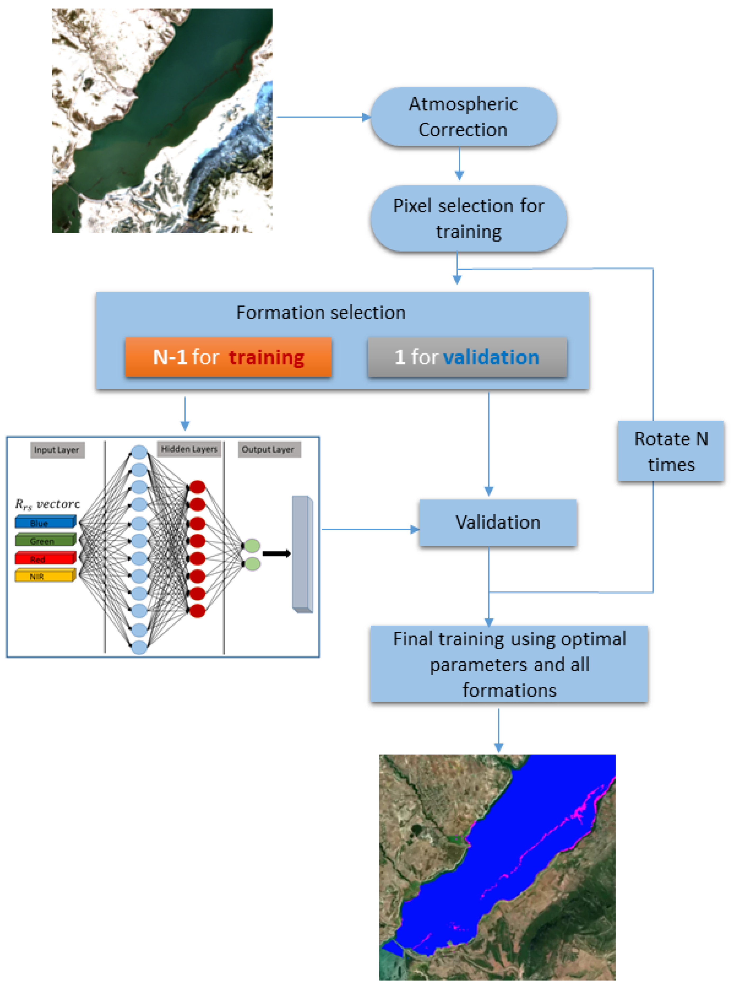
Figure 1.
Schematic showing the work flow of our methodology.
4. Experiments
4.1. Atmospheric Correction
The utility of an atmospheric correction algorithm (ACA) for pollutants detection will depend on two things: a) the technical characteristics of the output, and b) the quality of the correction (how accurate the correction is). The first encapsulates how many bands are processed and what is the horizontal resolution of the output. The horizontal resolution of the Sentinel-2 bands is not the same for all bands, and it differs between 10, 20 and 60m grid-spacing, which can be a limiting factor for some applications. For example, C2RCC generates the only for the first eight bands, which includes Narrow NIR (865 nm) but not NIR (832 nm). The generated output is given at 10 m pixels, even for the bands with an original pixel size of 20 or 60 meters. In contrast, iCOR generates for all MSI bands retaining the resolution of the original Sentinel-2 bands. Polymer, on the other hand, generates for all bands at 10 meters resolution. The only exception is the 2nd SWIR band (2202 nm), which is not processed at all. Finally, ACOLITE generates for all available bands with a 10 m resolution, the later however is partially true. This is because, even though the generated output is given at 10 meter pixel size, the “visual resolution” is the same as the resolution of the initial MSI bands. This means, that for a 20 m band like B6 (704 nm), four 10 m pixels forming a square have relatively similar values forming visually one 20 m pixel, which cannot be distinguished into four 10 m pixels.
When it comes to the detection of our formations, ACOLITE performs well. All formations are clearly represented with anomalous in most bands. This representation, however, is not the same for all bands. For example, the first three bands (443, 493, 560 nm) represent these formations with reduced anomalies compared to the surrounding clear water, and the remaining bands represent the formations with increased anomalies (Figure 2). This is illustrated in the representation of the 18 Jan 2021 oil spill with the Green (560 nm) and NIR band (Figure 3 and Figure 4, respectively). This transition, however, from negative to positive anomalies means that there is a wavelength where this transition takes place, and this can result in a lack of detection capability for bands that are close to this spectral threshold. This is exactly what happens during the 30 Dec 2017 event where the Red band does not exhibit a specific pattern that resembles these formations (Figure 5), indicating a lack of detection capability for that particular event. This doesn’t happen though for the other two cases, where the formation can be clearly identified in the Red band. Regarding the ability of the corrected bands to detect the formations, we must look at the band sensitivity. For ACOLITE the rule is that the highest sensitivity is achieved with NIR and Narrow NIR (Figure 2) indicating their detection potential. In fact the sensitivity increases as the wave length increases from 443 nm to the NIR region, and again decreases as we move into the SWIR region.
On the other hand, when it comes to iCOR, for the 18th Jan 2021 event, the bands show a similar behavior with that of ACOLITE (Figure 2). The formations are represented with reduced values in the lower part of the MSI spectrum, and with increased values in the medium and higher part, with the maximum again taking part in the NIR region. It is only for the weak formations of 2017, where things differ. In this case, the first three bands (Coastal Aerosol, Blue and Green) exhibit increased values of for the polluted pixels. Such inconsistency can add uncertainty in any detection method. Another limitation of iCOR is the spectral diversity of the processed image that is required for the algorithm to run properly. This is exactly what happen during the 18 Jan 2021 event, where the land surrounding our lake was fully covered with snow, which may have affected the atmospheric correction in ways that are unknown at this point and therefore could not be addressed in this study. Regarding the sensitivity of the iCOR corrected bands, it is several times (from 2 to 7) greater compared to that of ACOLITE (Figure 2, Figure 3 and Figure 4) indicating a greater detection potential.
C2RCC on the other hand, identifies the pollutants only with negative anomalies (Figure 2, Figure 3 and Figure 4). However, despite its advantage to output the first eight bands at the highest possible resolution (10 m), it also has severe limitations for this applications. This is because parts of the formations are automatically masked out, especially those where the formations are relatively thicker or more intense. This is particularly the case for the 18th January 2021 event, which gives the formation land-like optical properties, and are identified by C2RCC as land. This is because C2RCC is an atmospheric correction based on neural nets, which are trained based on a large sample of waters to estimate water optical properties suitable to detect water pigments, i.e. chl-a and TSM. Hence because of this it is only valid for water bodies. This could be seen as a limitation for our application given that the most intense parts of the formations are not identified as such. Another disadvantage of C2RCC is that its detection capability varies. For example, it can clearly detect the formation of 18 Jan 2021 (even by masking it as land), but it is unable to detect the one from 30 Dec 2017. Overall, it has a maximum sensitivity in the 560 nm range, rapidly decreasing to zero as we move in the Red Edge and NIR spectral region.
Unlike the first three ACAs, Polymer has a much lower ability to detect such formations overall. The pixels identified are represented by rather weak anomalies. Additionally, these values do not exhibit a robust structure (or they do not form a cluster of uniformly anomalous values that contrast the surrounding clear water). This happens across bands, and it can be clearly seen for the 18 Jan 2021 event (Figure 4), where the pollutants are less defined compared to those seem in and . However, this is not unjustified, given that Polymer relies on a water reflectance model based on Chl and it is simply not designed for polluted water. Both Polymer and C2RCC work pixel-by-pixel making assumptions about the water reflectance without using the entire MSI image. On the other hand, ACOLITE and iCOR make use of the whole image (land and water).
Given that the ultimate goal is to use to detect formations of unknown origin, the question is which algorithm should be used for the correction, and which bands are best for this. Our results clearly show that only iCOR and ACOLITE corrected bands have the potential to successfully detect the pollution events in question. However, iCOR exhibits some inconsistency regarding the type of anomaly our formations are represented with, which raises the uncertainty level, leading us to suggest ACOLITE as a better atmospheric correction for such applications. Regarding the band choice, this depends on the band resolution, the higher the resolution the higher its usage, especially for small events. Therefore the recommendation is to use, the four 10 m resolution bands (Red, Green, Blue, NIR). However, in the future, the use of the 20m bands should not be ruled out, given that ACOLITE gives the possibility of using these bands for detection. In the future we could also combine bands from different algorithms.
4.2. Parameter Learning and Optimization
Our study focuses on formations that were onserved during 30 Dec 2017 and 18 Jan 2021 in order to thoroughly examine these specific cases. Given the limitation of the small number of formations during these two days, it would be hard to implement an object based algorithm, which requires a relatively large number of similar formations for training. Therefore, a pixel based neural network algorithm was implemented instead.
The first step is to create the training dataset. For this, we create false color images (FCI), and we observe the identified formations. The FCI are generated by combining three atmospherically corrected bands (Red, Green and NIR), which offer the highest possible resolution and detection capacity. Five orthogonal patches that depict such formations are chosen (roughly 100x100 pixels each), three from the first image (30 Dec 2017) and another two from the second one (18 Jan 2021). Figure 6a and Figure 7a illustrate two of the formations used in our study, one from each Sentinel-2 image. Then the pixels corresponding to each formation from each patch are annotated via visual inspection as 1 and an equal number of pixels corresponding to clear water are labeled as 0 (Figure 6b and Figure 7b). Applying the above resulted in 5 groups of oil spill pixels with 108, 74, 75, 156, and 137 number of pixels each. Additionally, given that the first MSI image contained only very small formations, we artificially generated patches that were the result of smaller patches puzzled together to form a larger one for practical reasons (Figure 6a). The annotation applied to these formations could not include the entire extent of the formations for two reasons. First, some parts exhibit a relatively weak color contrast with the environment and could not be distinguished from the surrounding clear water. This is true mostly in the periphery of the formations where the pollution layer is relatively thin. Second, inclusion of pixels with very weak color contrast with clear water, could make our model too sensitive and could lead to an increased false positive rate, that had to be avoided.
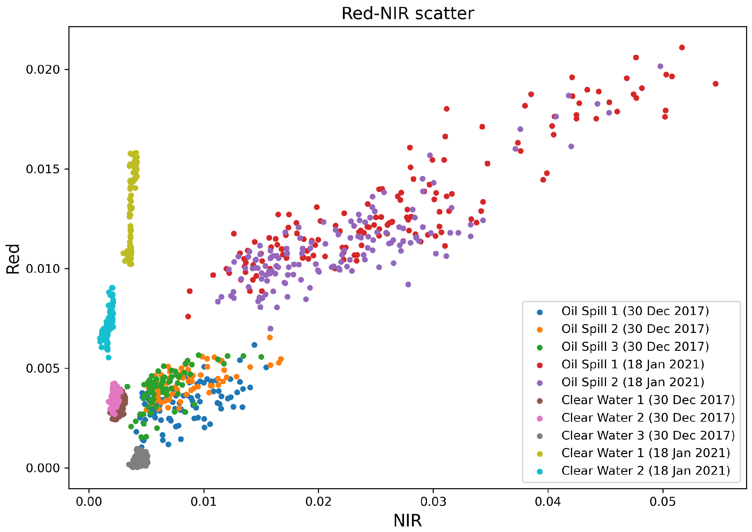
One thing to note here is that the pixels corresponding to the formations chosen from the two images had different characteristics, forming two distinct groups or values in all bands (Figure 8, scatterplot). This means that the two pixel groups had to be carefully balanced numerically, otherwise the training of the DNN on values predominantly from one group would result in a model that might fail to detect pixels corresponding to the other group.
We conduct three types of experiments. In the first, two vectors containing the corresponding Green and NIR values are fed to the algorithm along with the proper label. In the second, we use Red and NIR instead and in the third we use all four 10 m bands (492, 560, 665, and 832 nm). In each case, we implement a Deep Neural Network (DNN) with two hidden layers and an output layer. The hidden layers have 12 and 8 units, and they use a Relu activation. The output layer uses a sigmoid activation and has only two output classes. The DNN is run with eight different learning rates (ranging from 0.00005 to 0.1), a batch size of 10 and with 100 epochs. Two different optimizers are tested, Adam and SGD. Given the fact that every time we run the model the weights of the Neural Network are randomly initialized, leading to a different result, we run the model 10 times with the same combination of hyperparameters. At the end we estimate the final result by averaging our metrics from these 10 different experiments.
4.3. Results
Initially, we take five identified and annotated formations (observed during 30 Dec 2017 and 18 Jan 2021) from the Sentinel-2 images and we operate a 5-fold validation process, where each time we use four of the formations to train the algorithm and the last one is used for testing. We do this five times, while the formations rotate into testing mode. The metrics we employ to measure the performance of the algorithm are false positive rate, IoU, and accuracy. The results share common characteristics for all three types of experiments. First, only the Adam optimizer performs adequately. On the other hand, the SGD optimizer fails to accurately predict the formations in almost every run, either due to a large number of FPs or due to complete lack of detection capability. Second, the optimal learning rate is roughly in the range (0.0005-0.001) for the IoU and (0.00005-0.0001) for the FPR.
When it comes to the optimal band combination for detecting the formations, it seems that the 4-Band combination outperforms any of the 2 band combinations, with the Red-NIR being the least successful. More specifically, the best results (after we average over all formations) the DNN achieves during training are 0.04, 71.18 and 99.46% for the FPR, IoU, and accuracy, respectively. Figure 6c and Figure 7c show examples of the DNN prediction for two individual formations. A comparison of the annotation with the DNN prediction shows that the model captures the formations very well, also evident in the three metrics used.

Table 1.
IoU and FPR results corresponding to the validation runs for the 4 Bands, Red-NIR and Green-NIR experiments. Values represent averages across the five rotational runs.
Table 1.
IoU and FPR results corresponding to the validation runs for the 4 Bands, Red-NIR and Green-NIR experiments. Values represent averages across the five rotational runs.
| 4 Bands | Green-NIR | Red-NIR | ||||
| LR | IoU | FPR | IoU | FPR | IoU | FPR |
| 0.1 | 7.48 | 30.5 | 7.41 | 28.03 | 1.48 | 32 |
| 0.05 | 12.7 | 30.43 | 15.83 | 30.13 | 18 | 18.26 |
| 0.01 | 43.08 | 1.79 | 54.64 | 0.74 | 54.37 | 0.82 |
| 0.005 | 46.84 | 1.8 | 62.94 | 0.63 | 58.15 | 0.93 |
| 0.001 | 60.43 | 0.93 | 69.82 | 0.42 | 63.09 | 0.8 |
| 0.0005 | 71.18 | 0.4 | 68.76 | 0.27 | 58.41 | 0.65 |
| 0.0001 | 33.78 | 0.05 | 40.88 | 0.05 | 31.09 | 0.21 |
| 0.00005 | 26.44 | 0.03 | 29.92 | 0.05 | 28.31 | 0.04 |
Additionally, the perfect model is not expected to have a zero FPR, in fact a number of FP’s is naturally expected, and these represent the prediction of formation pixels that were not included in the annotation. This is perfectly captured in Figure 6a,b, where it is evident that a number of pixels depicting these formations are not included in the annotation, and are not included in the training either, leading to a model that fails to detect the formation in its entirety.
Regarding the use of atmospheric correction specifically designed for water applications, the question is whether this step is necessary. To answer this, we perform similar experiments where Level 2 Sentinel-2 images are used instead (called No Correction from now on). Note that for these images the default algorithm (Sen2cor) is applied. Our results indicate that the use of ACOLITE allows far better metrics (IoU, FPR, Accuracy) during the 5-fold validation step. Furthermore, the 4 Band and the Green-NIR band combination perform slightly better compared to the Red-NIR configuration, which is in general similar compared to the case where the ACOLITE algorithm has been used.
The purpose of this algorithm is to be used operationally to detect similar formations. One of the biggest concerns in such cases is when an algorithm gives too often false alarms, predicting formations when there are none. Therefore, after the validation process and the final training of the algorithm using the optimal hyperparameters and including all formations in our training set, the model is tested to a number of Sentinel-2 images (28 images corresponding to 28 different dates) where no formations are present. The results show that the algorithm does not produce any false positives indicating its potential for operational use.
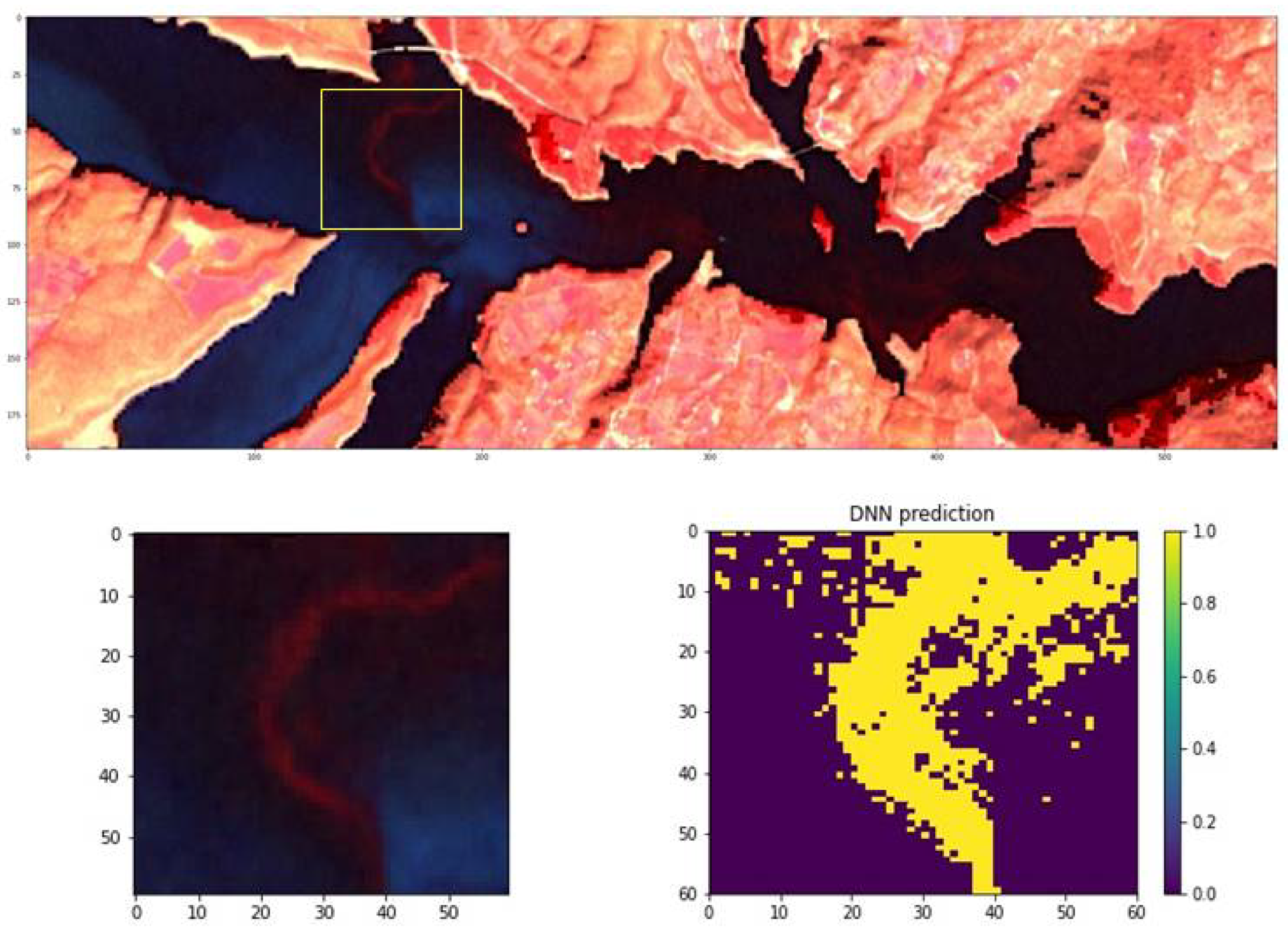
To further evaluate the prediction skill of our algorithm we use the oil spill case from an inland lake in Italy (lake Pertusillo) published in Lavene et al (2022). This event was chosen given its similarity (optically) to our formations. This particular study mentions several Sentinel-2 images that might contain oil spills due to inland oil drilling activity. Before running the DNN algorithm all images were processed with ACOLITE to correct for the atmospheric effect. It turns out that our trained DNN does have some detection skill, especially for the 27 Feb 2017 case where wide spread oil contamination is present (and verified) throughout the lake. On the other hand, for other cases mentioned in the Lavene et al. (2022) study, the model does not exhibit the same detection skill and it detects no oil spills. It should be noted though that some of these Sentinel-2 images are referred to as “suspect” images, and are not accompanied by in situ measurements that could verify the presence of hydrocarbons. Another thing that should be noted is that lake Pertusillo experiences algae blooms during the same time with the confirmed oil spills, affecting the visible part of the spectrum. This could explain why these oil spills do not have the same optical properties as the ones from Polyphytos reservoir. For example, maximum sensitivity is associated with the Red Edge bands. Additionally, for the wide spread oil spill of 27 Feb 2017, the boundaries of the oil spill can only be discerned in the Red Edge and NIR part of the spectrum. The lack of sensitivity of the visible bands to oil spills could be partly responsible for the lack of detection skill given that three out of the four bands our algorithm uses are from the VIS spectrum. In conclusion, training a universal algorithm for the detection of such formations in inland waters, would require a large number of such events covering a broad range of water types, which is not available at the moment.
Figure 9.
Sentinel-2 false color image (Green-Red-NIR) showing the oil spill case for the 27th February 2017 along with the DNN prediction.
Figure 9.
Sentinel-2 false color image (Green-Red-NIR) showing the oil spill case for the 27th February 2017 along with the DNN prediction.
5. Conclusions
This study focuses on the detection of formations of unknown origin (pollutants or even possible oil spills) on an inland lake. We use a pixel based deep neural network algorithm that uses multispectral images from Sentinel-2 satellite to detect these formations. Ten meter bands, RGB (visible) and NIR are used in different combinations and are fed into the algorithm as input data. The resulting model is capable of detecting these formations with good accuracy, however, it produces too many false positives by predicting pollutants when there are none. To solve this, we implement atmospheric correction methods that are specifically designed for water applications. Out of the 4 algorithms tested, ACOLITE is chosen as the most suitable. Its use allows the model to predict the pollutants with greater accuracy, as indicated by the metrics used. However, the model appears to be too “stringent“, given that it fails to detect these formations in their full extent. Thus, we conclude that the use of atmospheric correction algorithms in combination with DNNs in general improves the detection capability of the algorithm. Future improvements in the correction method though would certainly benefit the detection by allowing a better annotation and training of the model on more accurate observations.
Author Contributions
Conceptualization, Ilias Gialampoukidis, I. Lioumbas, A. Christodoulou; methodology, Damianos Mantsis; software, Natasa Moumtzidou; validation, Damianos Mantsis; formal analysis, Damianos Mantsis; investigation, Damianos Mantsis; resources, Damianos Mantsis, Anastasia Moumtzidou, I. Gialampoukidis; data curation, Anastasia Moumtzidou, I. Lioumbas, A. Christodoulou; writing—original draft preparation, Damianos Mantsis; writing—review and editing, Anastasia Moumtzidou, I. Gialampoukidis, I. Lioumbas, A. Christodoulou; visualization, Damianos Mantsis; supervision, Anastasia Moumtzidou, Ilias Gialampoukidis; project administration, S. Vrochidis, and I. Kompatsiaris; funding acquisition, S. Vrochidis, and I. Kompatsiaris. All authors have read and agreed to the published version of the manuscript.
Data Availability Statement
In this section, please provide details regarding where data supporting reported results can be found, including links to publicly archived datasets analyzed or generated during the study. Please refer to suggested Data Availability Statements in section “MDPI Research Data Policies” at https://www.mdpi.com/ethics. If the study did not report any data, you might add “Not applicable” here.
Acknowledgments
This research was funded by European Union’s Horizon 2020 Research and Innovation Program aqua3S, under Grant Agreement No 832876.
Conflicts of Interest
The authors declare no conflict of interest.
Abbreviations
The following abbreviations are used in this manuscript:
| NIR | Near Infra Red |
| SAR | Synthetic Aperture Radar |
| DNN | Deep Neural Network |
References
- Brekke, C.; Solberg, A. H. . Oil spill detection by satellite remote sensing. Remote Sens. of Env. 2005, 95(1), 1–13. [Google Scholar] [CrossRef]
- Brockmann, C., and Caouthors. Evolution of the C2RCC neural network for Sentinel-2 and 3 for the retrieval of ocean color products in normal and extreme optically complex waters. 2016.
- Solberg, A. H.; Brekke, C.; Husoy, P. O. Oil spill detection in Radarsat and Envisat SAR images. IEEE Trans. Geosci. Remote Sens 2007, 45, 746–755. [Google Scholar] [CrossRef]
- Topouzelis, K. Oil spill detection by SAR images: Dark formation detection, feature extraction and classification algorithms. Sensors 2008, 8, 6642–6659. [Google Scholar] [CrossRef] [PubMed]
- Solberg, A. H. Remote sensing of ocean oil-spill pollution. Proc. IEEE 2012, 100, 2931–2945. [Google Scholar] [CrossRef]
- Rajendran, S.; P. Vethamony; F. N. Sadooni; H. A. Al-Kuwari; J. A. Al-Khayat; H. Govil; and S. Nasir. Sentinel-2 image transfromation methods for mapping oil spill-A case study with Wakashio oil spill in the Indian Ocean, off Mauritius. MethodsX 2021, 8, 101327. [Google Scholar] [CrossRef] [PubMed]
- Lioumbas, J.; A. Christodoulou; M. Katsiapi; N. Xanthopoulou; P. Stournara; T. Spahos; G. Seretoudi; A. Mentes; N. Theodoridou. Satellite remote sensing to improve source water quality monitoring: A water utility’s perspective. Remote Sens. Appl.: Soc. Environ., 2023, 10, 101561. [Google Scholar]
- Sun, S.; C. Hu; L. Feng; G. A. Swayze; J. Holmes; G. Graettinger; I. MacDonald; O. Garcia; and I. Leifer. Oil slick morphology derived from AVIRIS measurements of the Deepwater Horizon oil spill: Implications for spatial resolution requirements of remote sensors. Marine Pollution Bull. 2016, 103, 276–285. [Google Scholar] [CrossRef]
- Fingas, M. F.; Brown, C. E. Review of oil spill remote sensing. Marine Pollution Bull. 2014, 83(1), 9–23. [Google Scholar] [CrossRef]
- Fingas, M.F.; Brown, C.E. A review of oil spill remote sensing. Sensors 2017, 18. [Google Scholar] [CrossRef]
- Nguyen, T. T. H.; T. P. T. Nguyen; K. Koike; M. T. Nhuan. Selecting the best band ratio to estimate Chlorophyll-a concentration in a tropical freshwater lake using Sentinel-2A images from a case study of lake Ba Be (North Vietnam). Int. J. of Geo-Information 2017, 6.
- Minchew, B.; Jones, C. E.; Holt, B. Polarimetric analysis of backscatter from the Deemwater Horizon oil spills using L-band synthetic aperture radar. IEEE Transactions on Geoscience and Remote Sens. 2012, 50. [Google Scholar]
- Singha, S.; Ressel, R.; Velloto, D.; Lehner, S. A combination of traditional and polarimetrric features for oil spill detection using TerraSAR-X. IEEE Journal of Selected Topics in Applied Earth Obs. and Remote Sens. 2016. [Google Scholar] [CrossRef]
- Fingas, M. F.; Brown, C. E. Review of oil spill remote sensing. Spill Science and Technology Bulletin 1997, 4(4), 199–208. [Google Scholar] [CrossRef]
- Espedal, H. A.; Johannessen, O. M. Cover: detection of oil spills near offshore installations using synthetic aperture radar (SAR). Int. J. Remote Sens. 1997, 21, 2141–2144. [Google Scholar] [CrossRef]
- Kapustin, I. A.; and Coauthors. On capabilities of tracking marine surface currents using artificial film slicks. Remote Sens. 2019, 11, 840. [Google Scholar] [CrossRef]
- Solberg, A. S.; Storvik, G.; Solberg, R.; Volden, E. Automatic detection of oil spills in ERS SAR images. IEEE Trans. Geosci. Remote Sens. 1999, 37, 1916–1924. [Google Scholar] [CrossRef]
- Liu, P.; Zhao, C.; Li, X.; He, M.; Pichel, W. Identification of ocean oil spills in SAR imagery based on fuzzy logic algorithm. Int. Journal of Remote Sens. 2010, 31, 4819–4833. [Google Scholar] [CrossRef]
- Konstantinidou, E. E.; Kolokoussis, P.; Topouzelis, K.; Moutzouris-Sidiris, I. An open source approach for oil spill detection using Sentinel-1 SAR images. 7th International Conference on Remote Sensing and Geoinformation of the Environment 2019, Paphos, Cyprous. [Google Scholar]
- Singha, S.; Vespe, M.; Trieschmann, O. Automatic Synthetic Aperture Radar based oil spill detection and performance estimation via a semi-automatic operation service benchmark. Marine Pollution Bull. 2013. [Google Scholar] [CrossRef]
- Zakzouk, M.; and Coauthors. Novel oil spill indices for Sentinel-2 imagery: A case study of natural seepage in Qaruh Island, Kuwait. MethodsX 2024.
- Topouzelis, K.; Psyllos, A. Oil spill feature selection and classification using decision tree forest on SAR image data J. of Photogrammetry and Remote Sens. 2012, 68, 135–143. [Google Scholar] [CrossRef]
- Cantorna, D.; Dafonte, C.; Inglesias, A.; Arcay, B. Oil spill segmentation in SAR images using convolutional neural networks. A comparative analysis with clustering and logistic regression algorithms. App. Soft Computing Journal 2019, 84. [Google Scholar] [CrossRef]
- Zeng, K.; Wang, Y. A deep convolutional neural network for oil spill detection from spaceborne SAR images. Remote Sens. 2020, 12. [Google Scholar] [CrossRef]
- Guo, H.; Wu, D.; An, J. Discrimination of oil slicks and lookalikes in polarimetric SAR images using CNN. Sensors 2017, 17, 1837. [Google Scholar] [CrossRef] [PubMed]
- Ma, X.; Xu, J.; Wu, P.; Kong, P. Oil spill detection based on deep convolutional neural network using polarimetric scattering information from Sentinel-1 images. IEEE Transactions on Geosciences and Remote Sens. 2022, 60. [Google Scholar] [CrossRef]
- Zhu, Q.; and Coauthors. Oil spill contextual and boundary-supervised detection network based on marine SAR images. IEEE Transactions on Geosciences and Remote Sens. 2022, 60. [Google Scholar] [CrossRef]
- Lavene, G.; and Coauthors. Remote sensing detection of algal blooms in a lake impacted by petroleum hydrocarbons. Remote Sens. 2017, 14, 121. [Google Scholar]
- Kolokoussis, P.; Karathanassi, V. Oil spill detection and mapping using Sentinel-2 imagery. Journal Mar. Sci. Eng. 2018, 6. [Google Scholar] [CrossRef]
- Vanhellemeont, Q. . Adaptation of the dark spectrum fitting atmospheric correction for aquatic applications of the Landsat and Sentinel-2 archives. Remote Sens. of Env. 2019, 225, 175–192. [Google Scholar] [CrossRef]
Figure 2.
North-South cross section of the 18 Jan 2021 formation. For ACOLITE all corrected bands are displayed, and for iCOR only the 10 m bands are displayed.
Figure 2.
North-South cross section of the 18 Jan 2021 formation. For ACOLITE all corrected bands are displayed, and for iCOR only the 10 m bands are displayed.
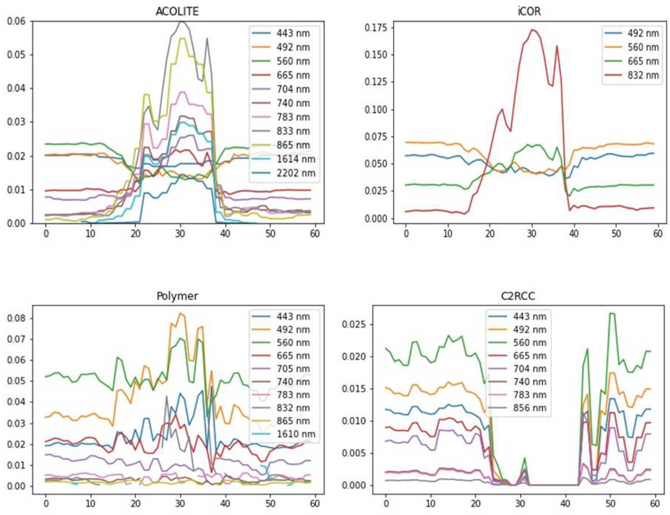
Figure 3.
Visualization of the 18 Jan 2021 formation with B5 (560 nm) after C2RCC, iCOR, Polymer, and ACOLITE corrections have been implemented. Note that the color bar is not the same for all images to improve direct comparison of formation characteristics after different atmospheric corrections have been applied.
Figure 3.
Visualization of the 18 Jan 2021 formation with B5 (560 nm) after C2RCC, iCOR, Polymer, and ACOLITE corrections have been implemented. Note that the color bar is not the same for all images to improve direct comparison of formation characteristics after different atmospheric corrections have been applied.
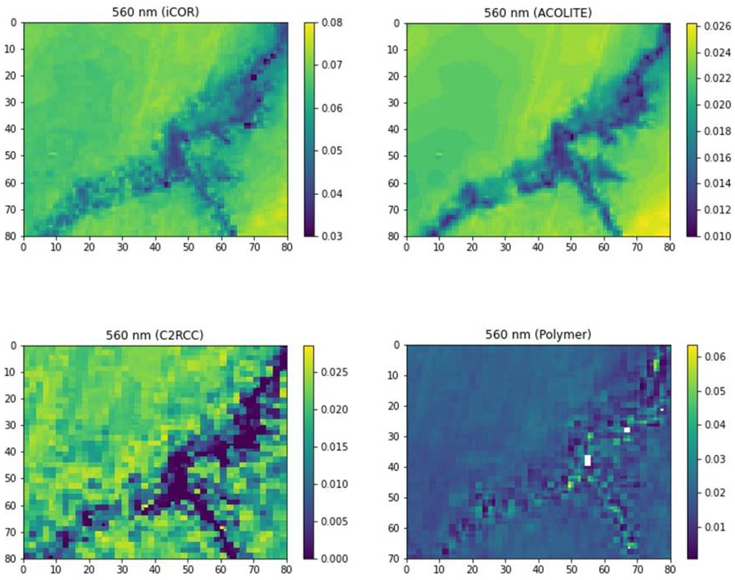
Figure 4.
Visualization of the 18 Jan 2021 formation with NIR (833 nm) after C2RCC, iCOR, Polymer, and ACOLITE corrections have been implemented. Note that for C2RCC we plot the 865 nm band, given that the NIR band is not available. Lack of data in the Polymer illustration indicates that the Polymer algorithm overestimates the correction resulting in a negative , and therefore is masked out.
Figure 4.
Visualization of the 18 Jan 2021 formation with NIR (833 nm) after C2RCC, iCOR, Polymer, and ACOLITE corrections have been implemented. Note that for C2RCC we plot the 865 nm band, given that the NIR band is not available. Lack of data in the Polymer illustration indicates that the Polymer algorithm overestimates the correction resulting in a negative , and therefore is masked out.
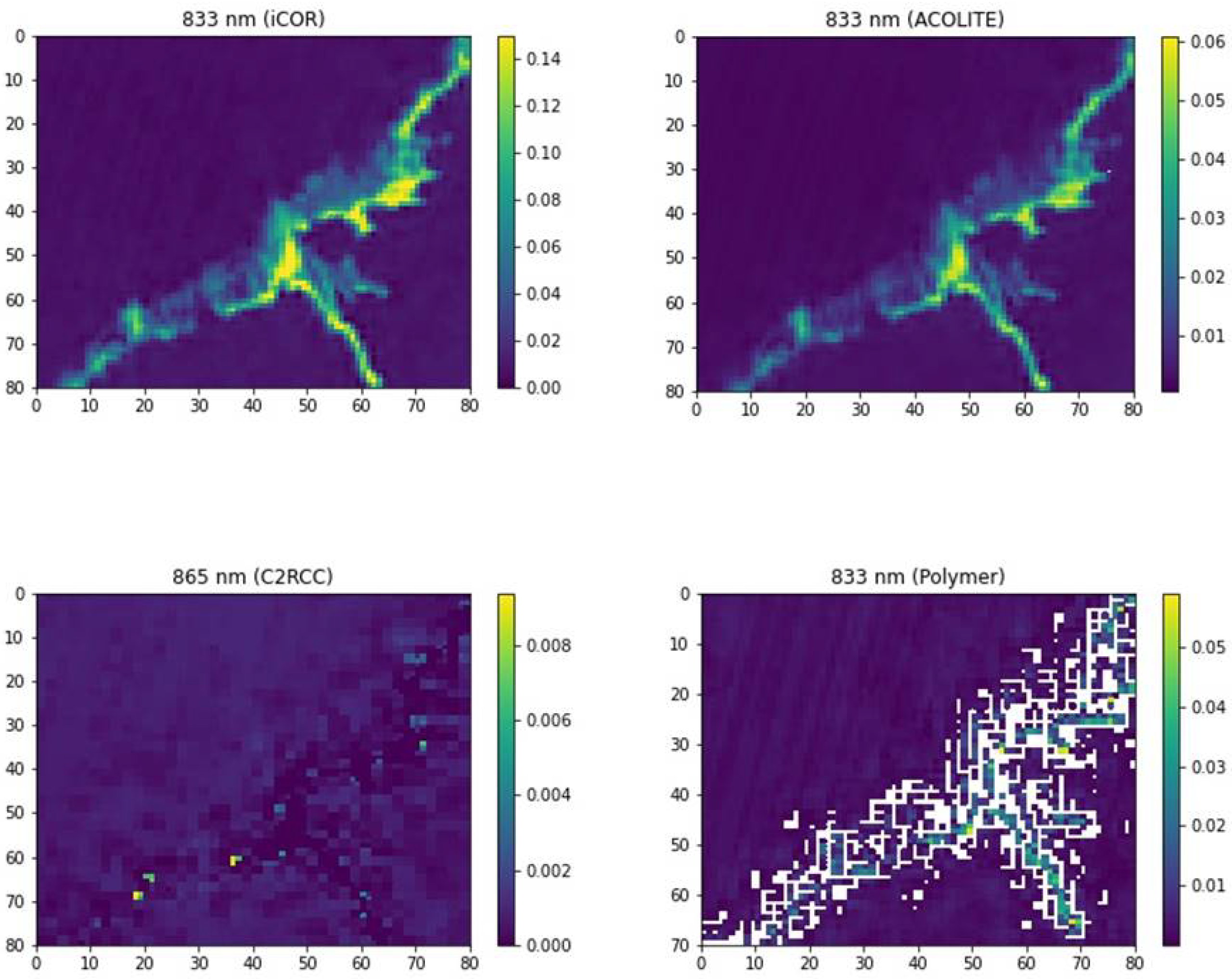
Figure 5.
Visualization of the 30 Dec 2017 formation with B4 (665 nm) after C2RCC, iCOR, Polymer, and ACOLITE corrections have been implemented. Note that the color bar scale is lower for C2RCC. The feature in the upper right corner represents land.
Figure 5.
Visualization of the 30 Dec 2017 formation with B4 (665 nm) after C2RCC, iCOR, Polymer, and ACOLITE corrections have been implemented. Note that the color bar scale is lower for C2RCC. The feature in the upper right corner represents land.
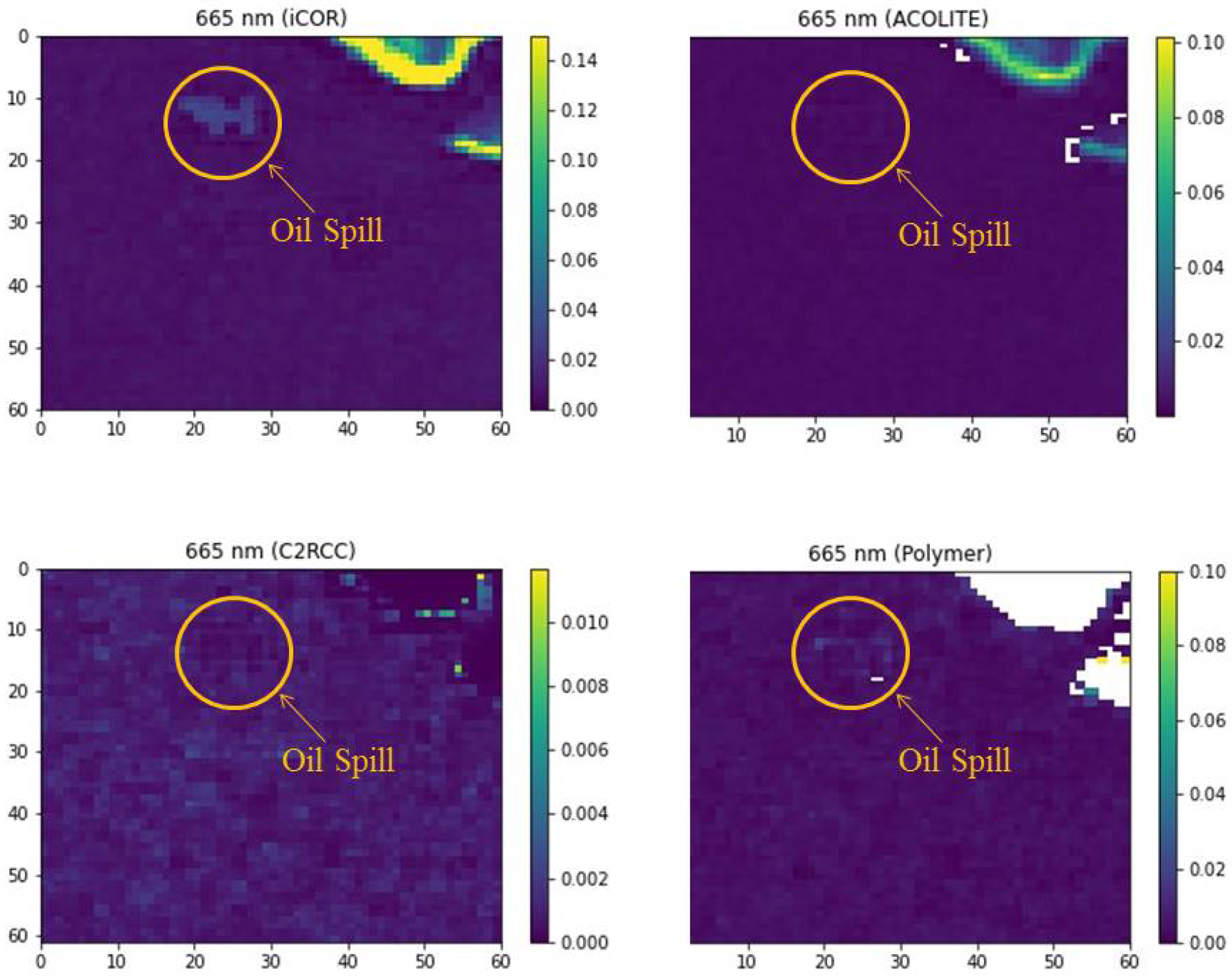
Figure 6.
a) False color image where three patches of different size (30 Dec 2017) were “puzzled together” to form one of the patches that was chosen for annotation, b) formation annotation, c) DNN prediction after ACOLITE was applied, and d) DNN prediction without ACOLITE.
Figure 6.
a) False color image where three patches of different size (30 Dec 2017) were “puzzled together” to form one of the patches that was chosen for annotation, b) formation annotation, c) DNN prediction after ACOLITE was applied, and d) DNN prediction without ACOLITE.
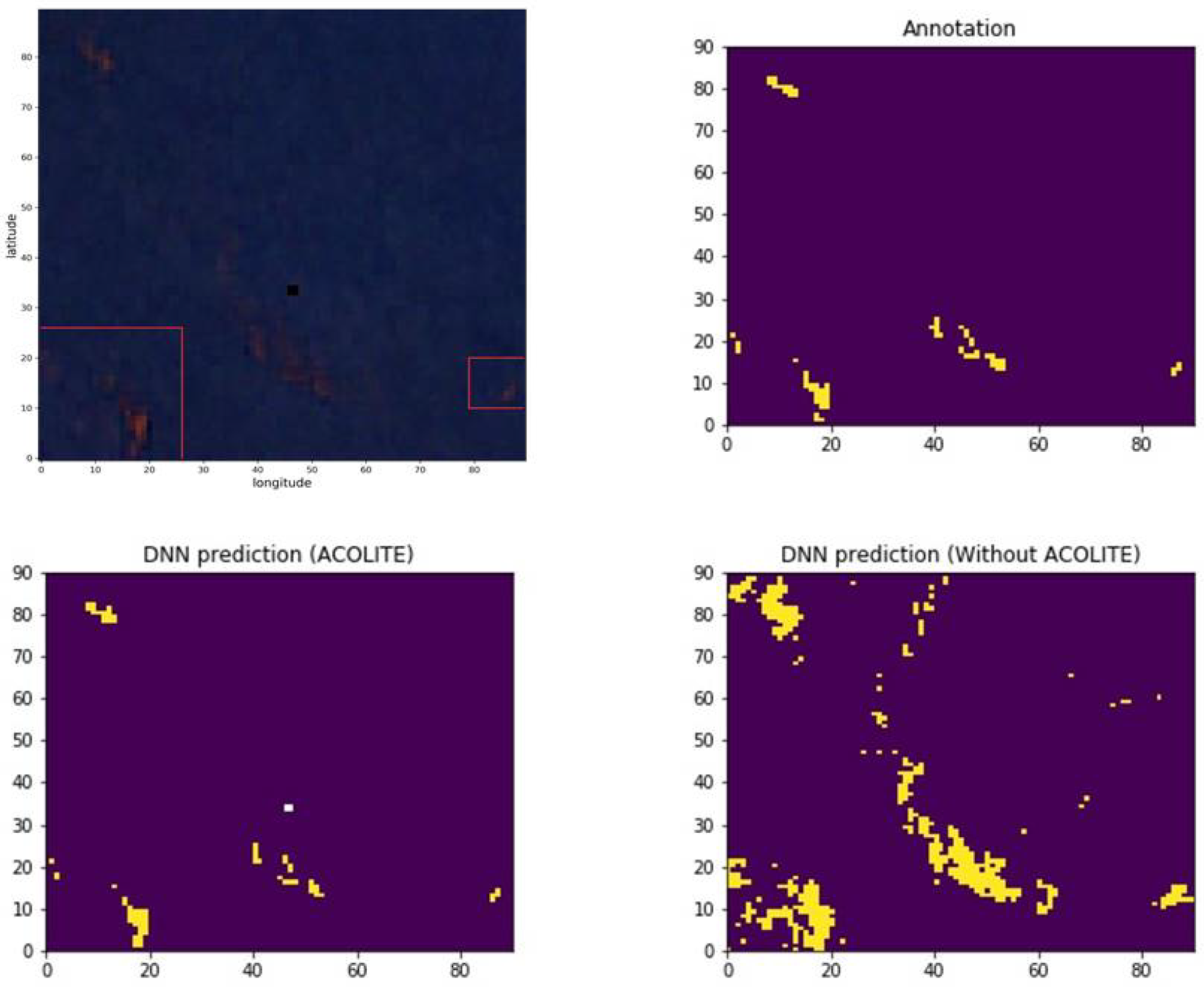
Figure 7.
a) False color image of one of the formations (18 Jan 2021) chosen for annotation, b) formation annotation, c) DNN prediction after ACOLITE was applied, and d) DNN prediction without ACOLITE.
Figure 7.
a) False color image of one of the formations (18 Jan 2021) chosen for annotation, b) formation annotation, c) DNN prediction after ACOLITE was applied, and d) DNN prediction without ACOLITE.
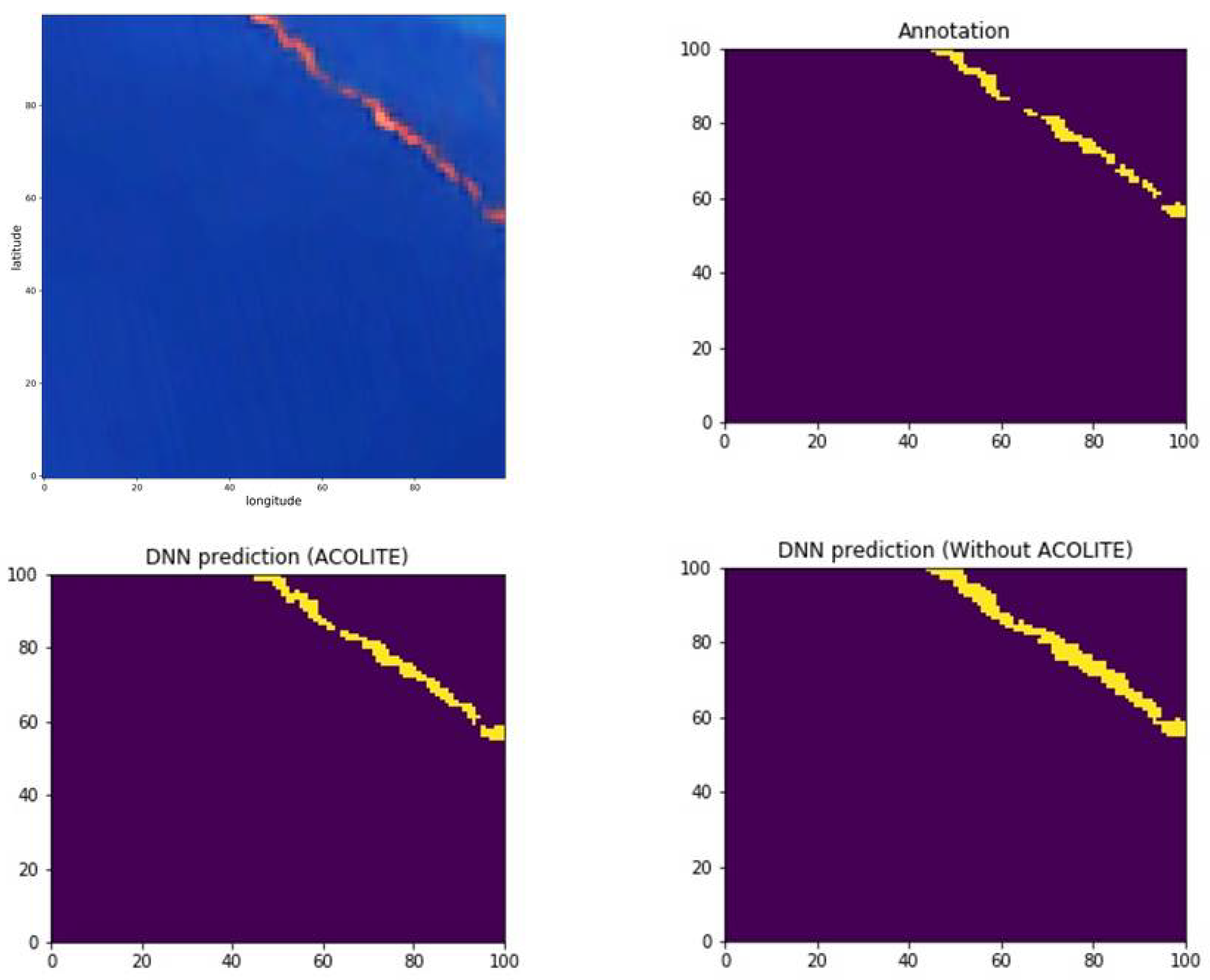
Figure 8.
Red-NIR scatterplot for the formation and clear water pixels that were annotated and used for the DNN training.
Figure 8.
Red-NIR scatterplot for the formation and clear water pixels that were annotated and used for the DNN training.
Disclaimer/Publisher’s Note: The statements, opinions and data contained in all publications are solely those of the individual author(s) and contributor(s) and not of MDPI and/or the editor(s). MDPI and/or the editor(s) disclaim responsibility for any injury to people or property resulting from any ideas, methods, instructions or products referred to in the content. |
© 2024 by the authors. Licensee MDPI, Basel, Switzerland. This article is an open access article distributed under the terms and conditions of the Creative Commons Attribution (CC BY) license (http://creativecommons.org/licenses/by/4.0/).
Copyright: This open access article is published under a Creative Commons CC BY 4.0 license, which permit the free download, distribution, and reuse, provided that the author and preprint are cited in any reuse.