High Order Difference Schemes for Space Riesz Variable-Order Nonlinear Fractional Diffusion Equations

Preprint

Article

High Order Difference Schemes for Space Riesz Variable-Order Nonlinear Fractional Diffusion Equations

Altmetrics

Downloads

Views

Comments

This version is not peer-reviewed

Submitted:

25 September 2024

Posted:

26 September 2024

You are already at the latest version

Alerts

Abstract

This article is aimed at studying new finite difference methods for one-dimensional (1D) and two-dimensional (2D) space Riesz variable-order (VO) nonlinear fractional diffusion equations (SRVONFDEs). In the presented model, fractional derivatives are defined in the Riemann-Liouville type. Based on 4-point weighted-shifted-Gr\"unwald-difference (4WSGD) operators for Riemann-Liouville constant-order (CO) fractional derivatives, which have a free parameter and have at least third order accuracy, we derive 4WSGD operators for space Riesz VO fractional derivatives. In order that the fully discrete schemes have good stability and can handle the nonlinear term efficiently, we apply the implicit Euler (IE) method to discretize the time derivative, which leads to IE-4WSGD schemes for SRVONFDEs. The stability and convergence of the IE-4WSGD schemes are analysed theoretically. In addiction, a parameter selection strategy is derived for 4WSGD schemes and banded preconditioners are put forward to accelerate the GMRES methods for solving the discretization linear systems. Numerical resutls demonstrate the effectiveness of the proposed schemes and preconditioners.

Keywords:

Subject: Computer Science and Mathematics - Computational Mathematics

MSC: 65M06; 26A33; 65M12

1. Introduction

Fractional differential equations have been successfully applied in many fields [2,3,4,36] and attracted many scientists. And many researchers investigated different numerical methods. Commonly used discretization methods include finite difference method, finite element method, and finite volume method [14,20,34]. In genearal, the discretization algebra systems are solved by certain preconditioned iteration methods; see for instance [18,35].

Since constant-order (CO) fractional differential equations fail to describe some complex transport diffusion processes [6,13], the variable-order fractional derivatives have be proposed and the variable-order fractional differential equations have received more and more attention [7,15,19,28,37,43]. Samko and Ross firstly gave the definition of variable-order (VO) fractional derivatives [32]. Lorenzo and Hartley derived different type of VO fractional calculus [21]. For applications of VO fractional differential equations, we refer readers to [15,37,43].

In recent years, many scholars have been studying approximate schemes for variable-order fractional differential equations. In [19], the relationship between the Riemann-Liouville VO fractional derivative and Grünwald-Letnikov expansion has been developed, and in [45], the first order explicit and implicit Euler methods are used to discretize variable-order fractional differential equations. Du, Alikhanov and Sun proposed a second order approximation scheme for time Caputo VO derivative by using special points on each time interval [10]. By utilizng the relationship between VO and CO fractional derivative, VO-WSGD operators for Riemann-Liouville VO fractional derivatives is derived, theory results suggest that the proposed schemes is greater than or equal to second order accuracy [17]. Here WSGD is the abbreviation of weighted-shifted-Grünwald-difference. Kheirkhah, Hajipour and Baleanu proposed a third-order WSGD formula to Caputo derivative for one-dimensional (1D) and two-dimensional (2D) time-fractional advection-reaction-subdiffusion equations with variable-order

α (x, t) \in (0, 1)

[16]. Wang, She, Lao and Lin proposed second-order FCD and fourth-order WSFCD operators for space Riesz VO nonlinear fractional diffusion equations (SRVONFDEs) [42]. However, the fourth-order WSFCD may cause stability problem if

α (x, t) \notin (1, - 3 + \sqrt[3]{48 + \sqrt{\frac{62207}{27}}} + \sqrt[3]{48 - \sqrt{\frac{62207}{27}}}) \approx (1, 1.6516) .

The aim of this work is to develop new difference schemes for the Riesz VO fractional derivative by 4-point weighted-shifted-Grünwald-difference (4WSGD) operators. Similar to [17,42], by applying the relationship between the Riesz CO and VO fractional derivatives, we obtain VO-4WSGD operators for Riesz VO fractional derivative. Then we employ the VO-4WSGD operators to SRVONFDEs.

In this paper, we first consider the following initial-boundary value (IBV) problem for a 1D SRVONFDE:

\begin{matrix} \{\begin{matrix} \frac{\partial u (x, t)}{\partial t} = K (x, t) \frac{\partial^{α (x, t)} u (x, t)}{\partial {| x |}^{α (x, t)}} + f (u, x, t), & (x, t) \in (a, b) \times (0, T], \\ u (x, 0) = u_{0} (x), & x \in (a, b), \\ u (a, t) = u_{a} (t) = 0, u (b, t) = u_{b} (t) = 0, & t \in [0, T], \end{matrix} \end{matrix}

(1)

where

0 < \underset{̲}{K_{C}} \leq K_{C} (x, t) = K (x, t) C_{α (x, t)} \leq \bar{K_{C}}

for certain positive constants

\underset{̲}{K_{C}}

and

\bar{K_{C}}

f (u, x, t)

is a nonlinear source term satisfying the Lipschitz condition

| f (u_{1}, x, t) - f (u_{2}, x, t) | \leq L | u_{1} - u_{2} |

for a certain positive constant L,

\frac{\partial^{α (x, t)} u (x, t)}{\partial {| x |}^{α (x, t)}}

denotes the

α (x, t)

th order Riesz VO fractional derivative (with regard to x) with

1 < \underset{̲}{α} \leq α (x, t) \leq \bar{α} < 2

. Here, the Riesz VO fractional derivative is defined by [30,45]

\frac{\partial^{α (x, t)} u (x, t)}{\partial {| x |}^{α (x, t)}} = C_{α (x, t)} [{}_{a}^{R}D_{x}^{α (x, t)} +_{x}^{R} D_{b}^{α (x, t)}] u (x, t), C_{α (x, t)} = - \frac{1}{2 cos \frac{π α (x, t)}{2}},

where

{}_{a}^{R}D_{x}^{α (x, t)}

and

{}_{x}^{R}D_{b}^{α (x, t)}

are the left-sided and right-sided Riemann-Liouville VO fractional derivatives defined by

{}_{a}^{R}D_{x}^{α (x, t)} u (x, t) = \frac{1}{Γ (2 - α (x, t))} {[\frac{d^{2}}{d ξ^{2}} \int_{a}^{ξ} \frac{u (η, t)}{{(ξ - η)}^{α (x, t) - 1}} d η]}_{ξ = x}, x \in (a, b),

{}_{x}^{R}D_{b}^{α (x, t)} u (x, t) = \frac{{(- 1)}^{2}}{Γ (2 - α (x, t))} {[\frac{d^{2}}{d ξ^{2}} \int_{ξ}^{b} \frac{u (η, t)}{{(η - ξ)}^{α (x, t) - 1}} d η]}_{ξ = x}, x \in (a, b) .

The 2D problem will be discussed in Section 5.

The rest of paper is organised as below. In Section 2, one gains VO-4WSGD operators for Riemann-Liouville VO fractional derivatives and analyze their accuracy. In Section 3, we obtain IE-4WSGD schemes for 1D SRVONFDE and derive stability and convergence. In Section 4, two banded preconditioners are proposed for the discrete systems of linear equations. The spectral radius and the condition number of the preconditioned systems are derived. Extension of the IE-4WSGD scheme to 2D SRVONFDE is discussed in Section 5. Numerical experiments are carried out in Section 6 to verify our theoretical results and concluding remarks are given in Section 7.

2. 4WSGD Operators for Riemann-Liouville VO Fractional Derivatives

Denote

α > 0

and

p \in N^{*}

, the shifted Grünword operator for the left-sided fractional derivative

{}_{- \infty}^{R}D_{x}^{α} u (x)

{}_{L}A_{h, p}^{α} u (x) = \frac{1}{h^{α}} \sum_{k = 0}^{\infty} g_{k}^{(α)} u (x - (k - p) h),

where

g_{k}^{(α)} = {(- 1)}^{k} i n o m α k

, i.e.,

g_{0}^{(α)} = 1, g_{k}^{(α)} = \frac{{(- 1)}^{k}}{k!} \prod_{j = 0}^{k - 1} (α - j), k = 1, 2, \dots .

(2)

As a matter of fact,

g_{k}^{(α)}

satisfies

{(1 - z)}^{α} = \sum_{k = 0}^{\infty} g_{k}^{(α)} z^{k}, | z | < 1 .

To approximate the left-sided Riemann-Liouville fractional derivative, the

{}_{L}A_{h, p}^{α}

has first-order accuracy:

{}_{L}A_{h, p}^{α} u (x) =_{- \infty}^{R} D_{x}^{α} u (x) + O (h);

(3)

see [22]. Similarly, for the right-sided Riemann-Liouville fractional derivative, the shifted Grünword operator is

{}_{R}A_{h, p}^{α} u (x) = \frac{1}{h^{α}} \sum_{k = 0}^{\infty} g_{k}^{(α)} u (x + (k - p) h)

and

{}_{R}A_{h, p}^{α} u (x) = {}_{x}^{R}D_{\infty}^{α} u (x) + O (h) .

In [34], a class of third-order 4WSGD operators are derived.

γ_{p} (p = - 1, 0, 1, 2)

represents the weights, and satisfies

\{\begin{matrix} γ_{2} = γ, \\ γ_{1} = \frac{3 α^{2} + 5 α}{24} - 3 γ, \\ γ_{0} = 1 + 3 γ + \frac{α - 3 α^{2}}{12}, \\ γ_{- 1} = \frac{3 α^{2} - 7 α}{24} - γ, \end{matrix}

(4)

where

γ

is a free parameter. The left 4WSGD operator is defined by

\begin{matrix} {}_{L}D_{h, γ}^{α} u (x) & = & γ_{2} \cdot {}_{L}A_{h, 2}^{α} u (x) + γ_{1} \cdot {}_{L}A_{h, 1}^{α} u (x) + γ_{0} \cdot {}_{L}A_{h, 0}^{α} u (x) + γ_{- 1} \cdot {}_{L}A_{h, - 1}^{α} u (x) \\ = \frac{1}{h^{α}} \sum_{k = 0}^{\infty} ω_{k, γ}^{(α)} u (x - (k - 2) h), \end{matrix}

(5)

where

ω_{k, γ}^{(α)} = γ_{2} g_{k}^{(α)} + γ_{1} g_{k - 1}^{(α)} + γ_{0} g_{k - 2}^{(α)} + γ_{- 1} g_{k - 3}^{(α)}

with

g_{- 1}^{(α)} = g_{- 2}^{(α)} = g_{- 3}^{(α)} = 0

and

g_{k}^{(α)}

for

k \geq 0

being defined by (2). Similarly, the right 4WSGD operator is defined by

\begin{matrix} {}_{R}D_{h, γ}^{α} u (x) = \frac{1}{h^{α}} \sum_{k = 0}^{\infty} ω_{k, γ}^{(α)} u (x + (k - 2) h) . \end{matrix}

(6)

The following theorem indicates that if the weights are given by (4) and

u (x)

is sufficiently smooth, then the the corresponding 4WSGD scheme has at least third-order accuracy.

Theorem 1.

[34] Assume

u (x) \in L^{1} (R) \cap C^{2} (R)

, and

{}_{- \infty}^{R}D_{x}^{α + 4} u (x)

{}_{x}^{R}D_{\infty}^{α + 4} u (x),

F [{}_{- \infty}D_{x}^{α + 4} u (x)] (R),

and

F [{}_{x}^{R}D_{\infty}^{α + 4} u (x)] (R) \in L^{1} (R)

, and

γ_{- 1}

γ_{0}

γ_{1}

γ_{2}

are given by (4), then

\begin{matrix} {}_{- \infty}^{R}D_{x}^{α} u (x) = {}_{L}D_{h, γ}^{α} u (x) + η_{L}, {}_{x}^{R}D_{\infty}^{α} u (x) = {}_{R}D_{h, γ}^{α} u (x) + η_{R}, \end{matrix}

where

| η_{L} | \leq C_{L} | γ - \frac{α^{3} - α^{2} - 4 α}{48} | h^{3} + O (h^{4}), | η_{R} | \leq C_{R} | γ - \frac{α^{3} - α^{2} - 4 α}{48} | h^{3} + O (h^{4})

with

C_{L}

and

C_{R}

being positive constants.

Remark 1.

From the inequalities for

| η_{L} |

and

| η_{R} |

, we know that the 4WSGD operators corresponding to

γ = \frac{α^{3} - α^{2} - 4 α}{48}

has fourth order accuracy. But the 4WSGD operator with 4th order may not suitable for variable-order fractional differential equations since it often causes stability problem.

Now we present the 4WSGD operator for the Riemann-Liouville VO fractional derivatives. According to the concept of Riemann-Liouville VO fractional derivatives, for each

α (x_{n}, t_{m})

, we can rewrite the definition as

\begin{matrix} {}_{a}^{R}D_{x}^{α (x_{n}, t_{m})} u (x, t_{m}) |_{x = x_{n}} & = & {[{}_{a}^{R}D_{ξ}^{α (x_{n}, t_{m})} u (ξ, t_{m})]}_{ξ = x_{n}}, \end{matrix}

(7)

\begin{matrix} {}_{x}^{R}D_{b}^{α (x_{n}, t_{m})} u (x, t_{m}) |_{x = x_{n}} & = & {[{}_{ξ}^{R}D_{b}^{α (x_{n}, t_{m})} u (ξ, t_{m})]}_{ξ = x_{n}} . \end{matrix}

(8)

The formulas (7)–(8) inspire an idea to develop 4WSGD operators for the Riemann-Liouville VO fractional derivatives. From (5) and (7), we get 4WSGD operators for

{}_{a}^{R}D_{x}^{α (x_{n}, t_{m})} u (x, t_{m}) |_{x = x_{n}}

\begin{matrix} {}_{L}D_{h, γ}^{α (x_{n}, t_{m})} u (x_{n}, t_{m}) & = & {[{}_{L}D_{h, γ}^{α (x_{n}, t_{m})} u (ξ, t_{m})]}_{ξ = x_{n}} \\ = & {[\frac{1}{h^{α (x_{n}, t_{m})}} \sum_{k = 0}^{\infty} ω_{k, γ}^{(α (x_{n}, t_{m}))} u (ξ - (k - 2) h, t_{m})]}_{ξ = x_{n}} \\ = & \frac{1}{h^{α (x_{n}, t_{m})}} \sum_{k = 0}^{\infty} ω_{k, γ}^{(α (x_{n}, t_{m}))} u (x_{n} - (k - 2) h, t_{m}), \end{matrix}

(9)

where

ω_{k}^{(α (x_{n}, t_{m}))}

are given by

ω_{k, γ}^{(α (x_{n}, t_{m}))} = γ_{2} g_{k}^{(α (x_{n}, t_{m}))} + γ_{1} g_{k - 1}^{(α (x_{n}, t_{m}))} + γ_{0} g_{k - 2}^{(α (x_{n}, t_{m}))} + γ_{- 1} g_{k - 3}^{(α (x_{n}, t_{m}))},

(10)

with

\{\begin{matrix} γ_{2} = γ, \\ γ_{1} = - 3 γ + \frac{3 α {(x_{n}, t_{m})}^{2} + 5 α (x_{n}, t_{m})}{24}, \\ γ_{0} = 3 γ + \frac{α (x_{n}, t_{m}) - 3 α {(x_{n}, t_{m})}^{2}}{12} + 1, \\ γ_{- 1} = - γ + \frac{3 α {(x_{n}, t_{m})}^{2} - 7 α (x_{n}, t_{m})}{24}, \end{matrix}

(11)

for

k = 0, 1, 2, \dots

. Here

\begin{matrix} g_{- 1}^{(α (x_{n}, t_{m}))} & = & g_{- 2}^{(α (x_{n}, t_{m}))} = g_{- 3}^{(α (x_{n}, t_{m}))} = 0, g_{0}^{(α (x_{n}, t_{m}))} = 1, \end{matrix}

(12)

\begin{matrix} g_{k}^{(α (x_{n}, t_{m}))} & = & \frac{{(- 1)}^{k}}{k!} \prod_{j = 0}^{k - 1} (α (x_{n}, t_{m}) - j), k = 1, 2, \dots . \end{matrix}

(13)

We refer readers to [17] for the idea of deriving formula (9). Similarly, 4WSGD operators for

{}_{x}^{R}D_{\infty}^{α (x_{n}, t_{m})} u (x, t_{m}) |_{x = x_{n}}

are

\begin{matrix} {}_{R}D_{h, γ}^{α (x_{n}, t_{m})} u (x_{n}, t_{m}) = \frac{1}{h^{α (x_{n}, t_{m})}} \sum_{k = 0}^{\infty} ω_{k, γ}^{(α (x_{n}, t_{m}))} u (x_{n} + (k - 2) h, t_{m}) . \end{matrix}

(14)

We call the formulas (9) and (14) left and right VO-4WSGD operator, respectively.

The zero extension of

u (x, t)

R \times [0, T]

\tilde{u} (x, t) = \{\begin{matrix} u (x, t), & (x, t) \in (a, b) \times [0, T], \\ 0, & else . \end{matrix}

Theorem 2.

Let

1 < \underset{̲}{α} \leq α (x, t) \leq \bar{α} < 2

and

u (x, t) \in L^{1} (R) \cap C^{2} (R)

, and

{}_{- \infty}^{R}D_{x}^{\bar{α} + 4} \tilde{u} (x, t)

{}_{x}^{R}D_{\infty}^{\bar{α} + 4} \tilde{u} (x, t)

and their Fourier transforms belong to

L^{1} (R)

. Let

{}_{L}D_{h, γ}^{α (x_{n}, t_{m})} \tilde{u} (x_{n}, t_{m})

and

{}_{R}D_{h, γ}^{α (x_{n}, t_{m})} \tilde{u} (x_{n}, t_{m})

be the VO-4WSGD operators given by (9) and (14), respectively. Then

\begin{matrix} {}_{- \infty}^{R}D_{x}^{α (x_{n}, t_{m})} \tilde{u} (x, t_{m}) |_{x = x_{n}} & = & {}_{L}D_{h, γ}^{α (x_{n}, t_{m})} \tilde{u} (x_{n}, t_{m}) + η_{L} (x_{n}, t_{m}), \\ {}_{x}^{R}D_{\infty}^{α (x_{n}, t_{m})} \tilde{u} (x, t_{m}) |_{x = x_{n}} & = & {}_{R}D_{h, γ}^{α (x_{n}, t_{m}))} \tilde{u} (x_{n}, t_{m})) + η_{R} (x_{n}, t_{m})), \end{matrix}

where

| η_{L} | \leq C_{L} | γ - \frac{α {(x_{n}, t_{m})}^{3} - α {(x_{n}, t_{m})}^{2} - 4 α (x_{n}, t_{m})}{48} | h^{3} + O (h^{4}),

| η_{R} | \leq C_{R} | γ - \frac{α {(x_{n}, t_{m})}^{3} - α {(x_{n}, t_{m})}^{2} - 4 α (x_{n}, t_{m})}{48} | h^{3} + O (h^{4})

with

C_{L}

and

C_{R}

being positive constants.

Proof.

Since

α (x, t) \in [\underset{̲}{α}, \bar{α}] \subset (1, 2)

, for given x and t, we have that

{}_{- \infty}^{R}D_{ξ}^{α (x_{n}, t_{m}) + 4} \tilde{u} (ξ, t_{m})

{}_{x}^{R}D_{\infty}^{α (x_{n}, t_{m}) + 4} \tilde{u} (ξ, t)

and their Fourier transforms belong to

L^{1} (R)

. Thus, for

α (x_{n}, t_{m})

, one gets by Theorem 1,

\begin{matrix} {}_{- \infty}^{R}D_{ξ}^{α (x_{n}, t_{m})} \tilde{u} (ξ, t_{m}) = {}_{L}D_{h, γ}^{α (x_{n}, t_{m})} \tilde{u} (ξ, t_{m}) + η_{L} (ξ, t_{m}) . \end{matrix}

In particular, by (7) we have

\begin{matrix} {}_{- \infty}^{R}D_{x}^{α (x_{n}, t_{m})} \tilde{u} (x, t_{m}) |_{x = x_{n}} & = & {[{}_{- \infty}^{R}D_{ξ}^{α (x_{n}, t_{m})} \tilde{u} (ξ, t_{m})]}_{ξ = x_{n}} \\ = & {[{}_{L}D_{h, γ}^{α (x, t)} \tilde{u} (ξ, t_{m}) + η_{L} (ξ, t)]}_{ξ = x_{n}} \\ = & {}_{L}D_{h, γ}^{α (x_{n}, t_{m})} \tilde{u} (x_{n}, t_{m}) + η_{L} (x_{n}, t_{m}), \end{matrix}

where

| η_{L} (x_{n}, t_{m}) | \leq C_{L} | γ - \frac{α {(x_{n}, t_{m})}^{3} - α {(x_{n}, t_{m})}^{2} - 4 α (x_{n}, t_{m})}{48} | h^{3} + O (h^{4}) .

Similarly, the relation between the right-sided Riemann-Liouville VO fractional derivative and the right-sided VO-4WSGD operator is obtained by using Theorem 1 and (8).□

Remark 2.

(i) Let

u (x, t)

be a function defined in

[a, b] \times [0, T]

with

u (a, t) = u (b, t) = 0

for

t \in [0, T]

, then

{}_{a}^{R}D_{x}^{α (x_{n}, t_{m})} u (x, t_{m}) |_{x = x_{n}}

can be approximated by

\begin{matrix} {}_{L}D_{h, γ}^{α (x_{n}, t_{m})} u (x_{n}, t_{m}) & = & \frac{1}{h^{α (x_{n}, t_{m})}} \sum_{k = 0}^{\infty} ω_{k, γ}^{(α (x_{n}, t_{m}))} u (x_{n} - (k - 2) h, t_{m}) \\ = & \frac{1}{h^{α (x_{n}, t_{m})}} \sum_{k = 0}^{⌊ (x_{n} - a) / h ⌋ + 2} ω_{k, γ}^{(α (x_{n}, t_{m}))} u (x_{n} - (k - 2) h, t_{m}), \end{matrix}

where

⌊ x ⌋

denotes the largest integer that is not greater than x. Similarly,

{}_{x}^{R}D_{b}^{α (x_{n}, t_{m})} u (x, t_{m}) |_{x = x_{n}}

can be approximated by

{}_{R}D_{h, γ}^{α (x_{n}, t_{m})} u (x_{n}, t_{m}) = \frac{1}{h^{α (x_{n}, t_{m})}} \sum_{k = 0}^{⌊ (b - x_{n}) / h ⌋ + 2} ω_{k, γ}^{(α (x_{n}, t_{m}))} u (x_{n} + (k - 2) h, t_{m}) .

(ii) Typically, for a discretization scheme that has good properties, the free parameter

γ

, which dependents on the value of

α (x, t)

, is of great importance.

3. IE-4WSGD Scheme for 1D SRVONFDE

3.1. IE-4WSGD Scheme

In this subsection, we derive IE-4WSGD schemes for the IBV problem of 1D SRVONFDE Eq (1). Let

N, M \in N^{*}

, and let

h = (b - a) / N

and

τ = T / M

, which represent the space grid size and the time step length, respectively. And denote

x_{n} = a + n h, n = 0, 1, 2, \dots N, t_{m} = m τ, m = 0, 1, 2, \dots M .

The following symbols are utilized

\begin{matrix} u_{n}^{m} = u (x_{n}, t_{m}), α_{n}^{m} = α (x_{n}, t_{m}), f_{e, n}^{m} = f (u (x_{n}, t_{m}), x_{n}, t_{m}), d_{n}^{m} = \frac{τ K_{C, n}^{m}}{h^{α_{n}^{m}}}, \\ {(_{a}^{R} D_{x}^{α_{n}^{m}} u)}_{n}^{m} = {}_{a}^{R}D_{x}^{α (x_{n}, t_{m})} u (x, t_{m}) |_{x = x_{n}}, {(_{x}^{R} D_{b}^{α_{n}^{m}} u)}_{n}^{m} = {}_{x}^{R}D_{b}^{α (x_{n}, t_{m})} u (x, t_{m}) |_{x = x_{n}} . \end{matrix}

Applying the implicit Euler (IE) formula

\frac{\partial u (x_{n}, t_{m})}{\partial t} = \frac{u (x_{n}, t_{m}) - u (x_{n}, t_{m - 1})}{τ} + O (τ)

to discretize

\frac{\partial u (x, t)}{\partial t}

, one gains

\begin{matrix} \frac{u_{n}^{m} - u_{n}^{m - 1}}{τ} = K_{C, n}^{m} [{(_{a}^{R} D_{x}^{α_{n}^{m}} u)}_{n}^{m} + {(_{x}^{R} D_{b}^{α_{n}^{m}} u)}_{n}^{m}] + f_{e, n}^{m} + O ({}_{τ}) . \end{matrix}

Approximating

{(_{a}^{R} D_{x}^{α_{n}^{m}} u)}_{n}^{m}

and

{(_{x}^{R} D_{b}^{α_{n}^{m}} u)}_{n}^{m}

by the left- and right-4WSGD operators respectively, and approximating

f (u_{n}^{m}, x_{n}, t_{m})

by the Taylor expansion, we get the following systems:

\begin{matrix} u_{n}^{m} & = & u_{n}^{m - 1} + \frac{τ K_{C, n}^{m}}{h^{α_{n}^{m}}} [\sum_{k = 0}^{n + 2} ω_{k, γ}^{(α_{n}^{m})} u_{n - k + 2}^{m} + \sum_{k = 0}^{N - n + 3} ω_{k, γ}^{(α_{n}^{m})} u_{n + k - 2}^{m}] + τ f_{e, n}^{m - 1} + τ R_{n}^{m}, \end{matrix}

where

n = 1, 2, \dots, N - 1, m = 1, 2, \dots, M

| R_{n}^{m} | \leq C (τ + h^{l})

for a certain constant

C > 0

with

l \in {3, 4}

Let the numerical approximation of

u_{n}^{m}

by the IE-4WSGD scheme be denoted by

U_{n}^{m}

and let

f_{n}^{m} = f (U_{n}^{m}, x_{n}, t_{m})

. By using

u_{0}^{m} = u_{N}^{m} = 0

u_{- 1}^{m} = u_{N + 1}^{m} = 0

, we obtain the linear equations about

{U_{n}^{m} : n = 1, 2, \dots, N - 1, m = 1, 2, \dots, M}

\begin{matrix} U_{n}^{m} - d_{n}^{m} [\sum_{k = 0}^{n + 2} ω_{k, γ}^{(α_{n}^{m})} U_{n - k + 2}^{m} + \sum_{k = 0}^{N - n + 3} ω_{k, γ}^{(α_{n}^{m})} U_{n + k - 2}^{m}] = U_{n}^{m - 1} + τ f_{n}^{m - 1} . \end{matrix}

(15)

Let

\begin{matrix} W_{L}^{m} & = & (\begin{matrix} ω_{2, γ}^{(α_{1}^{m})} & ω_{1, γ}^{(α_{1}^{m})} & ω_{0, γ}^{(α_{1}^{m})} & 0 & \dots & \dots & 0 \\ ω_{3, γ}^{(α_{2}^{m})} & ω_{2, γ}^{(α_{2}^{m})} & ω_{1, γ}^{(α_{2}^{m})} & ω_{0, γ}^{(α_{2}^{m})} & 0 & \dots & 0 \\ ⋮ & ⋱ & ⋱ & ⋱ & ⋱ & ⋱ & ⋮ \\ ⋮ & ⋮ & ⋱ & ⋱ & ⋱ & ⋱ & 0 \\ ⋮ & ⋮ & ⋱ & ⋱ & ⋱ & ⋱ & ⋮ \\ ω_{N - 1, γ}^{(α_{N - 2}^{m})} & ω_{N - 2, γ}^{(α_{N - 2}^{m})} & ω_{N - 3, γ}^{(α_{N - 2}^{m})} & ω_{N - 4, γ}^{(α_{N - 2}^{m})} & ⋱ & ω_{2, γ}^{(α_{N - 2}^{m})} & ω_{1, γ}^{(α_{N - 2}^{m})} \\ ω_{N, γ}^{(α_{N - 1}^{m})} & ω_{N - 1, γ}^{(α_{N - 1}^{m})} & ω_{N - 2, γ}^{(α_{N - 1}^{m})} & ω_{N - 3, γ}^{(α_{N - 1}^{m})} & \dots & ω_{3, γ}^{(α_{N - 1}^{m})} & ω_{2, γ}^{(α_{N - 1}^{m})} \end{matrix}), \end{matrix}

(16)

\begin{matrix} W_{R}^{m} & = & (\begin{matrix} ω_{2, γ}^{(α_{1}^{m})} & ω_{3, γ}^{(α_{1}^{m})} & ω_{4, γ}^{(α_{1}^{m})} & \dots & \dots & ω_{N - 1, γ}^{(α_{1}^{m})} & ω_{N, γ}^{(α_{1}^{m})} \\ ω_{1, γ}^{(α_{2}^{m})} & ω_{2, γ}^{(α_{2}^{m})} & ω_{3, γ}^{(α_{2}^{m})} & \dots & \dots & ω_{N - 2, γ}^{(α_{2}^{m})} & ω_{N - 1, γ}^{(α_{2}^{m})} \\ ω_{0, γ}^{(α_{3}^{m})} & ω_{1, γ}^{(α_{3}^{m})} & ω_{2, γ}^{(α_{3}^{m})} & \dots & \dots & ω_{N - 3, γ}^{(α_{3}^{m})} & ω_{N - 2, γ}^{(α_{3}^{m})} \\ 0 & ω_{0, γ}^{(α_{4}^{m})} & ω_{1, γ}^{(α_{4}^{m})} & ⋱ & \dots & ω_{N - 4, γ}^{(α_{4}^{m})} & ω_{N - 3, γ}^{(α_{4}^{m})} \\ ⋮ & ⋱ & ⋱ & ⋱ & ⋱ & ⋮ & ⋮ \\ ⋮ & ⋱ & ⋱ & ⋱ & ⋱ & ω_{2, γ_{N - 2}^{m}}^{(α_{N - 2}^{m})} & ω_{3, γ_{N - 2}^{m}}^{(α_{N - 2}^{m})} \\ 0 & \dots & \dots & 0 & ω_{0, γ}^{(α_{N - 1}^{m})} & ω_{1, γ}^{(α_{N - 1}^{m})} & ω_{2, γ}^{(α_{N - 1}^{m})} \end{matrix}), \end{matrix}

(17)

where

\begin{matrix} \begin{matrix} ω_{0, γ}^{(α_{j}^{m})} = γ_{j}^{m}, ω_{1, γ}^{(α_{j}^{m})} = - (3 + α_{j}^{m}) γ_{j}^{m} + \frac{3 {(α_{j}^{m})}^{2} + 5 α_{j}^{m}}{24}, \\ ω_{2, γ}^{(α_{j}^{m})} = \frac{{(α_{j}^{m})}^{2} + 5 α_{j}^{m} + 6}{2} γ_{j}^{m} - \frac{α_{j}^{m} (3 {(α_{j}^{m})}^{2} + 11 α_{j}^{m} - 2)}{24}, \\ ω_{k, γ}^{(α_{j}^{m})} = γ_{j}^{m} g_{k}^{(α_{j}^{m})} + (- 3 γ_{j}^{m} + \frac{3 {(α_{j}^{m})}^{2} + 5 α_{j}^{m}}{24}) g_{k - 1}^{(α_{j}^{m})} + (3 γ_{j}^{m} + \frac{α_{j}^{m} - 3 {(α_{j}^{m})}^{3}}{12} + 1) g_{k - 2}^{(α_{j}^{m})} \\ + (- γ_{j}^{m} + \frac{3 {(α_{j}^{m})}^{2} - 7 α_{j}^{m}}{24}) g_{k - 3}^{(α_{j}^{m})}, k \geq 3 . \end{matrix} \end{matrix}

(18)

Denote

D^{m} = diag (d_{1}^{m}, d_{2}^{m}, \dots, d_{N - 1}^{m}), U^{m} = {(U_{1}^{m}, U_{2}^{m}, \dots, U_{N - 1}^{m})}^{T}, F^{m} = {(f_{1}^{m}, f_{2}^{m}, \dots, f_{N - 1}^{m - 1})}^{T} .

We get the matrix form of Eq. (15):

A^{m} U^{m} = U^{m - 1} + τ F^{m - 1}, m = 1, 2, \dots, M,

(19)

where

\begin{matrix} A^{m} = I - D^{m} W^{m}, \end{matrix}

(20)

where

W^{m} = W_{L}^{m} + W_{R}^{m} .

Obviously,

W^{m} = {[w_{i j}^{m}]}_{i, j = 1}^{N - 1}

satisfy

w_{i j}^{m} = \{\begin{matrix} 2 ω_{2, γ}^{(α_{i}^{m})}, & j = i, \\ ω_{1, γ}^{(α_{i}^{m})} + ω_{3, γ}^{(α_{i}^{m})}, & j = i \pm 1, \\ ω_{0, γ}^{(α_{i}^{m})} + ω_{4, γ}^{(α_{i}^{m})}, & j = i \pm 2, \\ ω_{| i - j | + 2, γ}^{(α_{i}^{m})}, & | i - j | > 2 . \end{matrix}

(21)

3.2. Stability and Convergence Analysis

In this subsection, we analyze the stability and convergence of the IE-4WSGD scheme (15). We note that

W_{L}^{m}

W_{R}^{m}

and

W^{m}

are not Toeplitz matrices since the variable order

α (x, t)

depends on the space variable x (and the time variable t). Recalling that

D^{m}

are diagonal matrices with nonnegative entries, we put forward conditions for

W^{m}

to be diagonally dominant with negative diagonal entries, which is sufficient for the IE-4WSGD scheme to be stable.

Lemma 1.

[27,41] For

n = 0, 1, 2, . . ., N, m = 1, 2, . . ., M

and

α_{n}^{m} \in (1, 2),

the coefficient

{g_{k}^{(α_{n}^{m})}}_{k \geq 0}

satisfy

(i): $g_{0}^{(α_{n}^{m})} = 1, g_{1}^{(α_{n}^{m})} = - α_{n}^{m}, g_{k}^{(α_{n}^{m})} > 0 k \geq 2;$
(ii): $\sum_{k = 0}^{\infty} g_{k}^{(α_{n}^{m})} = 0, \sum_{k = 0}^{q} g_{k}^{(α_{n}^{m})} < 0, q \geq 1;$
(iii): $\frac{α_{n}^{m} (α_{n}^{m} - 1) (2 - α_{n}^{m}) (3 - α_{n}^{m})}{180} {(\frac{4}{k})}^{α_{n}^{m} + 1} < g_{k}^{(α_{n}^{m})} \leq \frac{α_{n}^{m} (α_{n}^{m} - 1)}{2} {(\frac{3}{k + 1})}^{α_{n}^{m} + 1}, k \geq 2;$
(iv): $\frac{(α_{n}^{m} - 1) (2 - α_{n}^{m}) (3 - α_{n}^{m})}{45} {(\frac{4}{k})}^{α_{n}^{m}} < \sum_{q = k}^{\infty} g_{q}^{(α_{n}^{m})} \leq \frac{(α_{n}^{m} - 1) 3^{α_{n}^{m} + 1}}{2 k^{α_{n}^{m}}}, k \geq 2;$
(v): $g_{k}^{(α_{n}^{m})} = O (k^{- (α_{n}^{m} + 1)}), k \geq 2$ .

Lemma 2.

Assume

1 < α_{n}^{m} < 2

and

ω_{k, γ}^{(α_{n}^{m})}

n = 0, 1, 2, . . ., N, m = 1, 2, . . ., M

, are given by (18). Then we have

\begin{matrix} \{\begin{matrix} ω_{0, γ}^{(α_{n}^{m})} = γ_{n}^{m}, ω_{1, γ}^{(α_{n}^{m})} = - (3 + α_{n}^{m}) γ_{n}^{m} + \frac{3 {(α_{n}^{m})}^{2} + 5 α_{n}^{m}}{24}, \\ ω_{2, γ}^{(α_{n}^{m})} = \frac{{(α_{n}^{m})}^{2} + 5 α_{n}^{m} + 6}{2} γ_{n}^{m} - \frac{α_{n}^{m} (3 {(α_{n}^{m})}^{2} + 11 α_{n}^{m} - 2)}{24}, \\ ω_{k, γ}^{(α_{n}^{m})} = (\frac{- {(α_{n}^{m})}^{3} - 6 {(α_{n}^{m})}^{2} - 11 α_{n}^{m} - 6}{k (k - 1) (k - 2)} γ_{n}^{m} \\ + \frac{24 k^{2} + (- 12 {(α_{n}^{m})}^{2} - 36 α_{n}^{m} - 96) k + (3 {(α_{n}^{m})}^{4} + 14 {(α_{n}^{m})}^{3} + 33 {(α_{n}^{m})}^{2} + 46 α_{n}^{m} + 72)}{24 (k - 1) (k - 2)}) g_{k - 3}^{(α_{n}^{m})}, k \geq 3, \\ \sum_{k = 0}^{\infty} ω_{k, γ}^{(α_{n}^{m})} = 0 . \end{matrix} \end{matrix}

(22)

Proof.

The formulas for

ω_{0, γ}^{(α_{i}^{m})}, ω_{1, γ}^{(α_{i}^{m})}

, and

ω_{2, γ}^{(α_{i}^{m})}

can be easily obtained from (11) and (18).

For

k \geq 3,

utilizing (13), we get

\begin{matrix} g_{k}^{(α_{n}^{m})} & = & \frac{k - 1 - α_{n}^{m}}{k} g_{k - 1}^{(α_{n}^{m})} = \frac{(k - 1 - α_{n}^{m}) (k - 2 - α_{n}^{m})}{k (k - 1)} g_{k - 2}^{(α_{n}^{m})} \\ = & \frac{(k - 1 - α_{n}^{m}) (k - 2 - α_{n}^{m}) (k - 3 - α_{n}^{m})}{k (k - 1) (k - 2)} g_{k - 3}^{(α_{n}^{m})} . \end{matrix}

Furthermore, by (10), we get

\begin{matrix} ω_{k, γ}^{(α_{n}^{m})} \\ = & γ_{n}^{m} g_{k}^{(α_{n}^{m})} + (- 3 γ_{n}^{m} + \frac{3 {(α_{n}^{m})}^{2} + 5 α_{n}^{m}}{24}) g_{k - 1}^{(α_{n}^{m})} + (3 γ_{n}^{m} + \frac{α_{n}^{m} - 3 {(α_{n}^{m})}^{3}}{12} + 1) g_{k - 2}^{(α_{n}^{m})} \\ + (- γ_{n}^{m} + \frac{3 {(α_{n}^{m})}^{2} - 7 α_{n}^{m}}{24}) g_{k - 3}^{(α_{n}^{m})} \\ = & (γ_{n}^{m} \frac{(k - 1 - α_{n}^{m}) (k - 2 - α_{n}^{m}) (k - 3 - α_{n}^{m})}{k (k - 1) (k - 2)} \\ + (- 3 γ_{n}^{m} + \frac{3 {(α_{n}^{m})}^{2} + 5 α_{n}^{m}}{24}) \frac{(k - 2 - α_{n}^{m}) (k - 3 - α_{n}^{m})}{(k - 1) (k - 2)}) g_{k - 3}^{(α_{n}^{m})} \\ + ((3 γ_{n}^{m} + \frac{α_{n}^{m} - 3 {(α_{n}^{m})}^{3}}{12} + 1) \frac{k - 3 - α_{n}^{m}}{k - 2} + (- γ_{n}^{m} + \frac{3 {(α_{n}^{m})}^{2} - 7 α_{n}^{m}}{24})) g_{k - 3}^{(α_{n}^{m})} \\ = & (\frac{- {(α_{n}^{m})}^{3} - 6 {(α_{n}^{m})}^{2} - 11 α_{n}^{m} - 6}{k (k - 1) (k - 2)} γ_{n}^{m} \\ + \frac{24 k^{2} + (- 12 {(α_{n}^{m})}^{2} - 36 α_{n}^{m} - 96) k + (3 {(α_{n}^{m})}^{4} + 14 {(α_{n}^{m})}^{3} + 33 {(α_{n}^{m})}^{2} + 46 α_{n}^{m} + 72)}{24 (k - 1) (k - 2)}) g_{k - 3}^{(α_{n}^{m})} . \end{matrix}

Finally, by Lemma 1 and Eq. (12), we get

\begin{matrix} \sum_{k = 0}^{\infty} ω_{k, γ}^{(α_{n}^{m})} \\ = & γ_{n}^{m} \sum_{k = 0}^{\infty} g_{k}^{(α_{n}^{m})} + (- 3 γ_{n}^{m} + \frac{3 {(α_{n}^{m})}^{2} + 5 α_{n}^{m}}{24}) \sum_{k = 0}^{\infty} g_{k - 1}^{(α_{n}^{m})} + (3 γ_{n}^{m} + \frac{α_{n}^{m} - 3 {(α_{n}^{m})}^{3}}{12} + 1) \sum_{k = 0}^{\infty} g_{k - 2}^{(α_{n}^{m})} \\ + (- γ_{n}^{m} + \frac{3 {(α_{n}^{m})}^{2} - 7 α_{n}^{m}}{24}) \sum_{k = 0}^{\infty} g_{k - 3}^{(α_{n}^{m})} \\ = & γ_{n}^{m} \sum_{k = 0}^{\infty} g_{k}^{(α_{n}^{m})} + (- 3 γ_{n}^{m} + \frac{3 {(α_{n}^{m})}^{2} + 5 α_{n}^{m}}{24}) \sum_{k = 0}^{\infty} g_{k}^{(α_{n}^{m})} + (3 γ_{n}^{m} + \frac{α_{n}^{m} - 3 {(α_{n}^{m})}^{3}}{12} + 1) \sum_{k = 0}^{\infty} g_{k}^{(α_{n}^{m})} \\ + (- γ_{n}^{m} + \frac{3 {(α_{n}^{m})}^{2} - 7 α_{n}^{m}}{24}) \sum_{k = 0}^{\infty} g_{k}^{(α_{n}^{m})} = 0 . \end{matrix}

□

Lemma 3.

Let

γ_{i}^{m}

be chosen such that

ω_{k, γ}^{(α_{i}^{m})}

k = 0, 1, 2, \dots

, satisfy

ω_{2, γ}^{(α_{i}^{m})} \leq 0, ω_{1, γ}^{(α_{i}^{m})} + ω_{3, γ}^{(α_{i}^{m})} \geq 0, ω_{0, γ}^{(α_{i}^{m})} + ω_{4, γ}^{(α_{i}^{m})} \geq 0, ω_{k, γ}^{(α_{i}^{m})} \geq 0, k \geq 5 .

(23)

Then

W^{m}

are diagonally dominant with negative diagonal entries.

Proof.

Consider the ith row of

W^{m}

. From (21) and (23), it can be seen that all diagonal entries

w_{i i}^{m} \leq 0

and all off-diagonal entries

w_{i j}^{m} \geq 0, i \neq j

. Thus, by Lemma 2, it is easily checked that

\begin{matrix} \sum_{j = 1}^{N - 1} {(W^{m})}_{i, j} = \sum_{j = 1}^{N - 1} w_{i j}^{m} \\ \leq & 2 ω_{2, γ}^{(α_{i}^{m})} + 2 (ω_{1, γ}^{(α_{i}^{m})} + ω_{3, γ}^{(α_{i}^{m})}) + 2 (ω_{0, γ}^{(α_{i}^{m})} + ω_{4, γ}^{(α_{i}^{m})}) + 2 \sum_{j = 5}^{\infty} ω_{j, γ}^{(α_{i}^{m})} \\ = & 2 \sum_{j = 0}^{\infty} ω_{j, γ}^{(α_{i}^{m})} = 0 . \end{matrix}

Equivalently,

\sum_{j = 1, j \neq i}^{\infty} w_{i j}^{m} \leq - w_{i i}^{m} = | w_{i i}^{m} | .

Therefore,

W^{m}

is diagonally dominant with negative diagonal entries. □

Theorem 3.

Let

α_{i}^{m} \in (1, 2)

i = 1, 2, . . ., N - 1, m = 1, 2, . . ., M

. If

γ_{i}^{m}

satisfies

\begin{matrix} {\tilde{γ}}_{3} (α_{i}^{m}) \leq γ_{i}^{m} \leq min {{\tilde{γ}}_{2} (α_{i}^{m}), {\tilde{γ}}_{4} (α_{i}^{m})} \end{matrix}

(24)

where

\{\begin{matrix} {\tilde{γ}}_{2} (α_{i}^{m}) = \frac{3 {(α_{i}^{m})}^{4} + 14 {(α_{i}^{m})}^{3} + 3 {(α_{i}^{m})}^{2} - 52 α_{i}^{m}}{8 ({(α_{i}^{m})}^{3} + 6 {(α_{i}^{m})}^{2} + 17 α_{i}^{m} + 24)}, \\ {\tilde{γ}}_{3} (α_{i}^{m}) = \frac{α_{i}^{m} [3 {(α_{i}^{m})}^{4} + 14 {(α_{i}^{m})}^{3} - 15 {(α_{i}^{m})}^{2} - 98 α_{i}^{m} + 72]}{6 ({(α_{i}^{m})}^{4} + 6 {(α_{i}^{m})}^{3} + 11 {(α_{i}^{m})}^{2} + 6 α_{i}^{m} + 24)}, \\ {\tilde{γ}}_{4} (α_{i}^{m}) = \frac{5 [3 {(α_{i}^{m})}^{4} + 14 {(α_{i}^{m})}^{3} - 27 {(α_{i}^{m})}^{2} - 134 α_{i}^{m} + 192]}{24 ({(α_{i}^{m})}^{3} + 6 {(α_{i}^{m})}^{2} + 11 α_{i}^{m} + 6)} . \end{matrix}

(25)

Then (23) holds, i.e.,

ω_{2, γ}^{(α_{i}^{m})} \leq 0, ω_{1, γ}^{(α_{i}^{m})} + ω_{3, γ}^{(α_{i}^{m})} \geq 0, ω_{0, γ}^{(α_{i}^{m})} + ω_{4, γ}^{(α_{i}^{m})} \geq 0, ω_{k, γ}^{(α_{i}^{m})} \geq 0, k \geq 5 .

Moreover, Eq. (24) has a solution for

α_{i}^{m} \in (1, α^{*})

, where

α^{*} \approx 1.83384978

(26)

is the unique solution of

3 μ^{8} + 32 μ^{7} + 42 μ^{6} - 556 μ^{5} - 1377 μ^{4} + 2204 μ^{3} + 2484 μ^{2} - 12048 μ + 23040 = 0 .

in the interval

(1, 2)

Proof.

For the sake of simplicity, we denote

α_{i}^{m}

μ

. According to Lemma 2, it can be seen that

ω_{2, γ}^{(μ)} = \frac{μ^{2} + 5 μ + 6}{2} γ_{i}^{m} - \frac{μ (3 μ^{2} + 11 μ - 2)}{24} \leq 0,

if and only if

γ_{i}^{m} \leq \frac{μ (3 μ^{2} + 11 μ - 2)}{12 (μ + 2) (μ + 3)} ≜ {\tilde{γ}}_{1} (μ) .

Notice that

\begin{matrix} ω_{1, γ}^{(μ)} + ω_{3, γ}^{(μ)} \\ = & - (3 + μ) γ_{i}^{m} + \frac{3 μ^{2} + 5 μ}{24} + \frac{- μ^{3} - 6 μ^{2} - 11 μ - 6}{6} γ_{i}^{m} + \frac{3 μ^{4} + 14 μ^{3} - 3 μ^{2} - 62 μ}{48} \\ = & - \frac{μ^{3} + 6 μ^{2} + 17 μ + 24}{6} γ_{i}^{m} + \frac{3 μ^{4} + 14 μ^{3} + 3 μ^{2} - 52 μ}{48}, \end{matrix}

it follows that

ω_{1, γ}^{(μ)} + ω_{3, γ}^{(μ)} \geq 0

if and only if

γ_{i}^{m} \leq \frac{3 μ^{4} + 14 μ^{3} + 3 μ^{2} - 52 μ}{8 (μ^{3} + 6 μ^{2} + 17 μ + 24)} ≜ {\tilde{γ}}_{2} (μ) .

\begin{matrix} ω_{0, γ}^{(μ)} + ω_{4, γ}^{(μ)} \\ = & γ_{i}^{m} + \frac{μ (μ^{3} + 6 μ^{2} + 11 μ + 6)}{24} γ_{i}^{m} - \frac{μ (3 μ^{4} + 14 μ^{3} - 15 μ^{2} - 98 μ + 72)}{144} \\ = & \frac{μ^{4} + 6 μ^{3} + 11 μ^{2} + 6 μ + 24}{24} γ_{i}^{m} - \frac{μ (3 μ^{4} + 14 μ^{3} - 15 μ^{2} - 98 μ + 72)}{144}, \end{matrix}

we see that

ω_{0, γ}^{(μ)} + ω_{4, γ}^{(μ)} \geq 0

if and only if

γ_{i}^{m} \geq \frac{μ (3 μ^{4} + 14 μ^{3} - 15 μ^{2} - 98 μ + 72)}{6 (μ^{4} + 6 μ^{3} + 11 μ^{2} + 6 μ + 24)} ≜ {\tilde{γ}}_{3} (μ) .

For

k \geq 5,

we have

\begin{matrix} ω_{k, γ}^{(μ)} & = & (\frac{- μ^{3} - 6 μ^{2} - 11 μ - 6}{k (k - 1) (k - 2)} γ_{i}^{m} \\ + \frac{24 k^{2} + (- 12 μ^{2} - 36 μ - 96) k + 3 μ^{4} + 14 μ^{3} + 33 μ^{2} + 46 μ + 72}{24 (k - 1) (k - 2)}) g_{k - 3}^{(μ)} . \end{matrix}

Notice that

g_{j}^{(μ)} > 0

for

j \geq 2

, we have that

w_{k, γ}^{(μ)} \geq 0

if and only if

γ_{i}^{m} \leq \frac{k [24 k^{2} + (- 12 μ^{2} - 36 μ - 96) k + 3 μ^{4} + 14 μ^{3} + 33 μ^{2} + 46 μ + 72]}{24 (μ^{3} + 6 μ^{2} + 11 μ + 6)} .

Let

\begin{matrix} g (x) & = & 24 x^{3} + (- 12 μ^{2} - 36 μ - 96) x^{2} + (3 μ^{4} + 14 μ^{3} + 33 μ^{2} + 46 μ + 72) x . \end{matrix}

It’s not difficult to verify that

g (x)

monotonically increases. Thus

g (k) \geq g (5)

for

k \geq 5

. In the other hand, for

k \geq 5,

we have

\begin{matrix} γ_{i}^{m} & \leq & \frac{5 [600 - 5 (12 μ^{2} + 36 μ + 96) + 3 μ^{4} + 14 μ^{3} + 33 μ^{2} + 46 μ + 72]}{24 (μ^{3} + 6 μ^{2} + 11 μ + 6)} \\ = & \frac{5 [3 μ^{4} + 14 μ^{3} - 27 μ^{2} - 134 μ + 192]}{24 (μ^{3} + 6 μ^{2} + 11 μ + 6)} ≜ {\tilde{γ}}_{4} (μ) . \end{matrix}

In the following, we will show that

{\tilde{γ}}_{1} (μ) \geq {\tilde{γ}}_{2} (μ) \geq {\tilde{γ}}_{3} (μ)

and derive the condition under which

{\tilde{γ}}_{3} (μ) \leq {\tilde{γ}}_{4} (μ)

(and therefore (24) holds).

We have

\begin{matrix} {\tilde{γ}}_{1} (μ) - {\tilde{γ}}_{2} (μ) \\ = & \frac{μ (3 μ^{2} + 11 μ - 2)}{12 (μ + 2) (μ + 3)} - \frac{3 μ^{4} + 14 μ^{3} + 3 μ^{2} - 52 μ}{8 (μ^{3} + 6 μ^{2} + 17 μ + 24)} \\ = & \frac{2 μ (3 μ^{2} + 11 μ - 2) (μ^{3} + 6 μ^{2} + 17 μ + 24)}{24 (μ + 2) (μ + 3) (μ^{3} + 6 μ^{2} + 17 μ + 24)} - \frac{3 (3 μ^{4} + 14 μ^{3} + 3 μ^{2} - 52 μ) (μ^{2} + 5 μ + 6)}{24 (μ + 2) (μ + 3) (μ^{3} + 6 μ^{2} + 17 μ + 24)} \\ = & \frac{- 3 μ^{6} - 29 μ^{5} - 43 μ^{4} + 353 μ^{3} + 1186 μ^{2} + 840 μ}{24 (μ^{4} + 8 μ^{3} + 29 μ^{2} + 58 μ + 48) (μ + 3)} \\ = & \frac{(- 3 μ^{5} - 20 μ^{4} + 17 μ^{3} + 302 μ^{2} + 280 μ) (μ + 3)}{24 (μ^{4} + 8 μ^{3} + 29 μ^{2} + 58 μ + 48) (μ + 3)} \\ = & \frac{- 3 μ^{5} - 20 μ^{4} + 17 μ^{3} + 302 μ^{2} + 280 μ}{24 (μ^{4} + 8 μ^{3} + 29 μ^{2} + 58 μ + 48)} . \end{matrix}

Let

{\tilde{γ}}_{12} (μ) = - 3 μ^{5} - 20 μ^{4} + 17 μ^{3} + 302 μ^{2} + 280 μ, μ \in (1, 2) .

Then

{\tilde{γ}}_{12}^{'} (μ) = - 15 μ^{4} - 80 μ^{3} + 51 μ^{2} + 604 μ + 280 .

It’s easy to check that

{\tilde{γ}}_{12}^{'} (μ) \geq 0

for

μ \in (1, 2) .

Thus

{\tilde{γ}}_{12} (μ)

monotonically increases. It follows that

{\tilde{γ}}_{12} (μ) \geq {\tilde{γ}}_{12} (1) = 576 > 0

for

μ \in (1, 2),

and therefore

{\tilde{γ}}_{1} (μ) \geq {\tilde{γ}}_{2} (μ) .

Next, we prove that

{\tilde{γ}}_{2} (μ) \geq {\tilde{γ}}_{3} (μ)

. We have

\begin{matrix} {\tilde{γ}}_{2} (μ) - {\tilde{γ}}_{3} (μ) \\ = & \frac{3 μ^{4} + 14 μ^{3} + 3 μ^{2} - 52 μ}{8 (μ^{3} + 6 μ^{2} + 17 μ + 24)} - \frac{μ (3 μ^{4} + 14 μ^{3} - 15 μ^{2} - 98 μ + 72)}{6 (μ^{4} + 6 μ^{3} + 11 μ^{2} + 6 μ + 24)} \\ = & \frac{{\tilde{γ}}_{23} (μ)}{24 (μ^{7} + 12 μ^{6} + 64 μ^{5} + 198 μ^{4} + 391 μ^{3} + 510 μ^{2} + 552 μ + 576)}, \end{matrix}

where

\begin{matrix} {\tilde{γ}}_{23} (μ) = - 3 μ^{8} - 32 μ^{7} - 120 μ^{6} - 74 μ^{5} + 1371 μ^{4} + 5722 μ^{3} + 3792 μ^{2} - 10656 μ . \end{matrix}

The derivative of

{\tilde{γ}}_{23} (μ)

\begin{matrix} {\tilde{γ}}_{23}^{'} (μ) = - 24 μ^{7} - 224 μ^{6} - 720 μ^{5} - 370 μ^{4} + 5484 μ^{3} + 17166 μ^{2} + 7584 μ - 10656 . \end{matrix}

It’s easy to check that

{\tilde{γ}}_{23}^{'} (μ) \geq 0,

μ \in (1, 2) .

Therefore,

{\tilde{γ}}_{23} (μ) \geq {\tilde{γ}}_{23} (1) = 18240 > 0, μ \in (1, 2) .

Hence,

{\tilde{γ}}_{2} (μ) \geq {\tilde{γ}}_{3} (μ) .

In order that (24) has a solution, it is required that

{\tilde{γ}}_{4} (μ) \geq {\tilde{γ}}_{3} (μ)

. By some computation, we get

\begin{matrix} {\tilde{γ}}_{4} (μ) - {\tilde{γ}}_{3} (μ) \\ = & \frac{5 (3 μ^{4} + 14 μ^{3} - 27 μ^{2} - 134 μ + 192)}{24 (μ^{3} + 6 μ^{2} + 11 μ + 6)} - \frac{μ (3 μ^{4} + 14 μ^{3} - 15 μ^{2} - 98 μ + 72)}{6 (μ^{4} + 6 μ^{3} + 11 μ^{2} + 6 μ + 24)} \\ = & \frac{{\tilde{γ}}_{34} (μ)}{24 (μ^{7} + 12 μ^{6} + 58 μ^{5} + 144 μ^{4} + 217 μ^{3} + 276 μ^{2} + 300 μ + 144)}, \end{matrix}

where

\begin{matrix} {\tilde{γ}}_{34} (μ) & = & 3 μ^{8} + 32 μ^{7} + 42 μ^{6} - 556 μ^{5} - 1377 μ^{4} + 2204 μ^{3} + 2484 μ^{2} - 12048 μ + 23040 . \end{matrix}

It is easy to get

\begin{matrix} {\tilde{γ}}_{34}^{'} (μ) = 24 μ^{7} + 224 μ^{6} + 252 μ^{5} - 2780 μ^{4} - 5508 μ^{3} + 6612 μ^{2} + 4968 μ - 12048 . \end{matrix}

We can verify that

{\tilde{γ}}_{34}^{'} (μ)

decreases for

μ \in (1, 2)

and it follows that

{\tilde{γ}}_{34}^{'} (μ) \leq {\tilde{γ}}_{34}^{'} (1) = - 8256 < 0 .

Therefore,

{\tilde{γ}}_{34} (μ)

also decreases. Notice that

{\tilde{γ}}_{34} (1) = 13824 > 0, {\tilde{γ}}_{34} (2) = - 5760 < 0,

we have that there exists a unique

α^{*} \in (1, 2)

such that

{\tilde{γ}}_{34} (α^{*}) = 0 .

By using Matlab, we get

α^{*} \approx 1.83384978

. Thus,

{\tilde{γ}}_{4} (μ) \geq {\tilde{γ}}_{3} (μ)

for

μ \in (1, α^{*}),

and (24) has solution(s). □

Lemma 4.

[1] (The barrier lemma) Assume

M_{A}

is a a monotone matrix with

M_{A} \in R^{n \times n} .

If there is a unit vector

\vec{ϱ}

, i.e.,

∥ \vec{ϱ} ∥_{\infty} = 1

, and

min_{1 \leq i \leq n} {(M_{A} \vec{ϱ})}_{i} \geq a_{M}

with

a_{M} > 0

a positive constant. Then one gains

∥ M_{A}^{- 1} ∥_{\infty} \leq 1 / a_{M} .

Define

e = {(1, 1, \dots, 1)}^{T}

. For any vectors

x, y \in R^{n}

, denote

x \geq (or >) y

{[x - y]}_{i} \geq 0

(or

{[x - y]}_{i} > 0

)

i = 1, 2, \dots, n

Lemma 5.

Suppose

1 < α_{i}^{m} \leq α^{*}

with

α^{*}

being given by (26) and

γ_{i}^{m}

is chosen such that

{\tilde{γ}}_{3} (α_{i}^{m}) \leq γ_{i}^{m} \leq min {{\tilde{γ}}_{2} (α_{i}^{m}), {\tilde{γ}}_{4} (α_{i}^{m})}

i = 1, 2, \dots, N - 1,

where

{\tilde{γ}}_{2} (α_{i}^{m}), {\tilde{γ}}_{3} (α_{i}^{m})

and

{\tilde{γ}}_{4} (α_{i}^{m})

are given by (25). Then

∥ {(A^{m})}^{- 1} ∥_{\infty} \leq 1

Proof.

Notice that

A^{m} = I - D^{m} W^{m}

with

W^{m}

given by (21), we are aware of that

A^{m}

is an L-matrix. By Lemmas 2 and 3, we have

\begin{matrix} \sum_{j = 1}^{N - 1} {[A^{m}]}_{i j} = 1 - d_{i}^{m} \sum_{j = 1}^{N - 1} w_{i j}^{(α_{i}^{m})} \\ \geq & 1 - [2 ω_{2, γ}^{(α_{i}^{m})} + 2 (ω_{1, γ}^{(α_{i}^{m})} + ω_{3, γ}^{(α_{i}^{m})}) + 2 (ω_{0, γ}^{(α_{i}^{m})} + ω_{4, γ}^{(α_{i}^{m})}) + 2 \sum_{j = 5}^{\infty} ω_{j, γ}^{(α_{i}^{m})}] \\ \geq & 1 - 2 \sum_{j = 0}^{\infty} ω_{j, γ}^{(α_{i}^{m})} \geq 1, i = 1, 2, \dots, N - 1 . \end{matrix}

Hence,

A^{m} e \geq e > 0 .

It follows that

A^{m}

is an M-matrix [12]. Furthermore,

∥ {(A^{m})}^{- 1} ∥_{\infty} \leq min_{1 \leq i \leq N} {[e]}_{i} = 1

from Lemma 4. □

Lemma 6.

[45] (Discrete Gronwall Inequality) Let

{ζ^{n} | n \geq 0}

be a sequence with

ζ^{n} > 0

, and

ϱ^{n} \geq 0 .

ζ^{n + 1} \leq (1 + c τ) ζ^{n} + τ ϱ^{n}, n = 0, 1, 2, \dots,

then

ζ^{n}

satisfies

ζ^{n + 1} \leq e^{c n τ} \sum_{k = 0}^{n} τ ϱ^{k},

where

ζ^{0} = 0,

c is a nonnegative constant.

Theorem 4.

1 < α_{i}^{m} \leq α^{*}

with

α^{*}

being given by (26) and

γ_{i}^{m}

is chosen such that

{\tilde{γ}}_{3} (α_{i}^{m}) \leq γ_{i}^{m} \leq min {{\tilde{γ}}_{2} (α_{i}^{m}), {\tilde{γ}}_{4} (α_{i}^{m})},

i = 1, 2, \dots, N - 1, m = 1, 2 \dots, M,

where

{\tilde{γ}}_{2} (α_{i}^{m}), {\tilde{γ}}_{3} (α_{i}^{m})

and

{\tilde{γ}}_{4} (α_{i}^{m})

are given by (25). Then the IE-4WSGD scheme (19) is stable.

Proof.

Suppose

{\tilde{U}}^{m}

is the approximation solution of

U^{m}

and

{\tilde{F}}^{m} = {({\tilde{f}}_{1}^{m}, {\tilde{f}}_{2}^{m}, \dots, {\tilde{f}}_{N - 1}^{m - 1})}^{T}

. Let

E^{m} = U^{m} - {\tilde{U}}^{m} .

Then we have

A^{m} E^{m} = E^{m - 1} + τ (F^{m - 1} - {\tilde{F}}^{m - 1}), m = 1, 2, \dots, M,

that is,

E^{m} = {(A^{m})}^{- 1} E^{m - 1} + τ {(A^{m})}^{- 1} (F^{m - 1} - {\tilde{F}}^{m - 1}) .

From Lemma 5, we get

\begin{matrix} ∥ E^{m} ∥_{\infty} & \leq & ∥ {(A^{m})}^{- 1} ∥_{\infty} ∥ E^{m - 1} ∥_{\infty} + τ L ∥ {(A^{m})}^{- 1} ∥_{\infty} {∥ E^{m - 1} ∥}_{\infty} \\ \leq & (1 + τ L) ∥ E^{m - 1} ∥_{\infty} \leq {(1 + τ L)}^{m} ∥ E^{0} ∥_{\infty} \leq e^{m τ L} ∥ E^{0} ∥_{\infty} \leq e^{T L} {∥ E^{0} ∥}_{\infty} . \end{matrix}

This can lead to the conclusion. □

Theorem 5.

Denote

u_{n}^{m}

the exact solution of IBV problem (1) and

U_{n}^{m}

the solution of (19). If

1 < α_{i}^{m} \leq α^{*}

and

{\tilde{γ}}_{3} (α_{i}^{m}) \leq γ_{i}^{m} \leq min {{\tilde{γ}}_{2} (α_{i}^{m}), {\tilde{γ}}_{4} (α_{i}^{m})},

i = 1, 2, \dots, N - 1, m = 1, 2, \dots, M .

Then for

1 \leq m \leq M

, it holds

∥ U^{m} - u^{m} ∥_{\infty} \leq C e^{T L} T (τ + h^{l}),

where

C > 0

and

l \in {3, 4}

Proof.

Denote

e^{m} = U^{m} - u^{m}

. From Eqs. (1) and (19), we get

A^{m} e^{m} = e^{m - 1} + τ (F_{e}^{m - 1} - F^{m - 1}) + τ R^{m}, m = 1, 2, \dots, M,

where

∥ R^{m} ∥_{\infty} \leq C (τ + h^{l}), l \in {3, 4} .

That is,

e^{m} = {(A^{m})}^{- 1} e^{m - 1} + τ {(A^{m})}^{- 1} (F_{e}^{m - 1} - F^{m - 1}) + τ {(A^{m})}^{- 1} R^{m} .

Notice that

e^{0} = 0,

from Lemmas 5 and 6, we get

\begin{matrix} ∥ e^{m} ∥_{\infty} & \leq & ∥ {(A^{m})}^{- 1} ∥_{\infty} ∥ e^{m - 1} ∥_{\infty} + τ L ∥ {(A^{m})}^{- 1} ∥_{\infty} ∥ e^{m - 1} ∥_{\infty} + τ ∥ {(A^{m})}^{- 1} ∥_{\infty} {∥ R^{m} ∥}_{\infty} \\ \leq & (1 + τ L) ∥ e^{m - 1} ∥_{\infty} + τ {∥ R^{m} ∥}_{\infty} \leq e^{m τ L} C m τ (τ + h^{l}) \leq C e^{T L} T (τ + h^{l}) . \end{matrix}

This can lead to the conclusion. □

In the following, we discuss how to choose the parameters

γ_{i}^{m}

such that the IE-4WSGD scheme is stable and has the optimal error bound.

Theorem 6.

Let

γ_{o b j} (α_{i}^{m}) = \frac{{(α_{i}^{m})}^{3} - {(α_{i}^{m})}^{2} - 4 α_{i}^{m}}{48}, i = 1, 2, \dots, N - 1, m = 1, 2, \dots, M

and let

α^{* *} \approx 1.79968326

(27)

be the unique solution of

- μ^{6} - 5 μ^{5} + 29 μ^{4} + 169 μ^{3} - 220 μ^{2} - 1316 μ + 1920 = 0

in the interval

(1, 2)

. Then for

α_{i}^{m} \in (1, α^{* *})

, it holds

{\tilde{γ}}_{3} (α_{i}^{m}) \leq γ_{o b j} (α_{i}^{m}) \leq min {{\tilde{γ}}_{2} (α_{i}^{m}), {\tilde{γ}}_{4} (α_{i}^{m})},

(28)

where

{\tilde{γ}}_{2} (α_{i}^{m}), {\tilde{γ}}_{3} (α_{i}^{m})

and

{\tilde{γ}}_{4} (α_{i}^{m})

are given by (25). That is, if

α (x, t) \in (0, α^{* *})

, then we can select the free parameter of the 4WSGD scheme so that the corresponding scheme has fourth order of accuracy.

Proof.

We first compare

γ_{o b j} (μ)

and

{\tilde{γ}}_{3} (μ)

. We have

\begin{matrix} γ_{o b j} (μ) - {\tilde{γ}}_{3} (μ) \\ = & \frac{μ^{3} - μ^{2} - 4 μ}{48} - \frac{μ (3 μ^{4} + 14 μ^{3} - 15 μ^{2} - 98 μ + 72)}{6 (μ^{4} + 6 μ^{3} + 11 μ^{2} + 6 μ + 24)} \\ = & \frac{γ_{o b j 3} (μ)}{48 (μ^{4} + 6 μ^{3} + 11 μ^{2} + 6 μ + 24)}, \end{matrix}

where

γ_{o b j 3} (μ) = μ^{7} + 5 μ^{6} - 23 μ^{5} - 141 μ^{4} + 94 μ^{3} + 736 μ^{2} - 672 μ .

It follows that

γ_{o b j 3}^{'} (μ) = 7 μ^{6} + 30 μ^{5} - 115 μ^{4} - 564 μ^{3} + 282 μ^{2} + 1472 μ - 672 .

It is easily checked that

γ_{o b j 3}^{'} (μ)

increases first and then decreases with

γ_{o b j 3}^{'} (1) > 0

and

γ_{o b j 3}^{'} (α^{*}) < 0

for

(1, α^{*})

. Thus

γ_{o b j 3} (μ)

also increases first and then decreases and there exists a minimum at

μ = 1

μ = α^{*} .

Since

γ_{o b j 3} (1) = 0,

γ_{o b j 3} (α^{*}) > 0,

therefore

γ_{o b j 3} (μ) \geq 0,

that is

γ_{o b j} (μ) \geq {\tilde{γ}}_{3} (μ)

for

(1, α^{*})

Next we compare

{\tilde{γ}}_{2} (μ)

and

γ_{o b j} (μ)

. We have

\begin{matrix} {\tilde{γ}}_{2} (μ) - γ_{o b j} (μ) \\ = & \frac{3 μ^{4} + 14 μ^{3} + 3 μ^{2} - 52 μ}{8 (μ^{3} + 6 μ^{2} + 17 μ + 24)} - \frac{μ^{3} - μ^{2} - 4 μ}{48} \\ = & \frac{γ_{o b j 2} (μ)}{48 (μ^{3} + 6 μ^{2} + 17 μ + 24)}, \end{matrix}

where

γ_{o b j 2} (μ) = - μ^{6} - 5 μ^{5} + 11 μ^{4} + 101 μ^{3} + 110 μ^{2} - 216 μ .

Then it is easy to get

γ_{o b j 2}^{'} (μ) = - 6 μ^{5} - 25 μ^{4} + 44 μ^{3} + 303 μ^{2} + 220 μ - 216,

and one can verify that

γ_{o b j 2}^{'} (μ)

increases monotonically for

μ \in (1, α^{*})

. Notice that

γ_{o b j 2}^{'} (1) = 320 > 0

, we have that

γ_{o b j 2} (μ) \geq γ_{o b j 2} (1) \geq 0 .

Equivalently,

{\tilde{γ}}_{2} (μ) \geq γ_{o b j} (μ)

for

(1, α^{*})

Finally, we compare

{\tilde{γ}}_{4} (μ)

and

γ_{o b j} (μ)

. We have

\begin{matrix} {\tilde{γ}}_{4} (μ) - γ_{o b j} (μ) \\ = & \frac{5 (3 μ^{4} + 14 μ^{3} - 27 μ^{2} - 134 μ + 192)}{24 (μ^{3} + 6 μ^{2} + 11 μ + 6)} - \frac{μ^{3} - μ^{2} - 4 μ}{48} \\ = & \frac{γ_{o b j 4} (μ)}{48 (μ^{3} + 6 μ^{2} + 11 μ + 6)}, \end{matrix}

where

γ_{o b j 4} (μ) = - μ^{6} - 5 μ^{5} + 29 μ^{4} + 169 μ^{3} - 220 μ^{2} - 1316 μ + 1920 .

It can be checked that

γ_{o b j 4}^{'} (μ) = - 6 μ^{5} - 25 μ^{4} + 116 μ^{3} + 507 μ^{2} - 440 μ - 1316

increases monotonically and

γ_{o b j 4}^{'} (α^{*}) < 0 .

Therefore,

γ_{o b j 4} (μ)

decreases monotonically. Notice that

γ_{o b j 4} (1) > 0 and γ_{o b j 4} (α^{*}) \leq 0,

we see that there exists a unique

α^{* *} \in (1, α^{*})

such that

γ_{o b j 4} (α^{* *}) = 0

. By using Matlab, we get an approximate value of

α^{* *}

, i.e.,

α^{* *} \approx 1.79968326

. That is

γ_{o b j 4} (μ) > 0

for

α_{i}^{m} \in (1, α^{* *})

, and

γ_{o b j 4} (α^{*}) < 0

for

α_{i}^{m} \in (α^{* *}, α^{*})

In summary,

{\tilde{γ}}_{3} (α_{i}^{m}) \leq γ_{o b j} (α_{i}^{m}) \leq min {{\tilde{γ}}_{2} (α_{i}^{m}), {\tilde{γ}}_{4} (α_{i}^{m})} α_{i}^{m} \in (1, α^{* *}) .

□

To end this section, we discuss how to choose the parameter

γ_{i}^{m}

for

α^{* *} < α_{i}^{m} \leq α^{*}

, where

α^{*}

and

α^{* *}

are given by (26) and (27) respectively. The minimization problem will take into account

\begin{matrix} min | γ_{i}^{m} - \frac{{(α_{i}^{m})}^{3} - {(α_{i}^{m})}^{2} - 4 α_{i}^{m}}{48} | \\ s . t . & {\tilde{γ}}_{3} (α_{i}^{m}) \leq γ_{i}^{m} \leq min {{\tilde{γ}}_{2} (α_{i}^{m}), {\tilde{γ}}_{4} (α_{i}^{m})}, α^{* *} \leq α_{i}^{m} \leq α^{*} . \end{matrix}

To seek above-mentioned problem, we draw the curves below (see Figure 1):

Objective: $γ_{o b j} (α_{i}^{m}),$
Lower bound: ${\tilde{γ}}_{3} (α_{i}^{m}),$
Upper bound: $min {{\tilde{γ}}_{2} (α_{i}^{m}), {\tilde{γ}}_{4} {(α)}_{i}^{m}} .$

Combining Theorem 6 and the curves in Figure 1, it can be easily seen that

{\tilde{γ}}_{4} (α_{i}^{m}) \leq γ_{o b j} (α_{i}^{m}), {\tilde{γ}}_{3} (α_{i}^{m}) \leq γ_{o b j} (α_{i}^{m})

for

[α^{* *}, α^{*})

, and

{\tilde{γ}}_{4} (α_{i}^{m})

is closer to the objective

{\tilde{γ}}_{o b j} (α_{i}^{m})

. Therefore, we can choose

γ_{i}^{m} = {\tilde{γ}}_{4} (α_{i}^{m})

for

[α^{* *}, α^{*}) .

In summary, select

γ_{i}^{m}

as follows:

γ_{i}^{m} = \{\begin{matrix} γ_{o b j} (α_{i}^{m}), α_{i}^{m} \in (1, α^{* *}) \\ {\tilde{γ}}_{4} (α_{i}^{m}), α_{i}^{m} \in [α^{* *}, α^{*}) . \end{matrix}

(29)

4. Preconditioning Techniques

In this section, based on Section 3, we consider applying preconditioned GMRES methods to solve the linear systems in Eq. (19). Although the coefficient matrices are dense and do not have a Toeplitz-like structure, each

W^{m}

has off-diagonal decay property, hence we employ banded matrices as preconditioners for the linear systems to speed up the relevant GMRES methods. Similar discussion can be found in the literature; see for instance [18,42].

Firstly, a banded preconditioner with diagonal compensation will be take into account. Letting

Q = {(q_{i j})}_{i, j = 1}^{N}

, we denote

diag (\sum_{j = 1}^{N} q_{1 j}, \sum_{j = 1}^{N} q_{2 j}, \dots, \sum_{j = 1}^{N} q_{N j})

diag (sum (Q, 2))

. Let

k_{b}

be an integer that is much less than N. Split

W^{m}

W^{m} = W_{k_{b}}^{m} + (W^{m} - W_{k_{b}}^{m}),

where

W_{k_{b}}^{m} = {\tilde{W}}_{k_{b}}^{m} + diag (sum (W^{m} - {\tilde{W}}_{k}^{m}, 2))

with

{\tilde{W}}_{k_{b}}^{m} = (\begin{matrix} w_{1, 1}^{(m)} & \dots & w_{1, k_{b}}^{(m)} & 0 & \dots & 0 \\ ⋮ & ⋱ & ⋮ & ⋱ & ⋱ & ⋮ \\ w_{k_{b}, 1}^{(m)} & \dots & w_{k_{b}, k_{b}}^{(m)} & ⋱ & ⋱ & 0 \\ 0 & ⋱ & ⋱ & ⋱ & ⋱ & w_{N - k_{b}, N - 1}^{(m)} \\ ⋮ & ⋱ & ⋱ & ⋱ & ⋱ & ⋮ \\ 0 & \dots & 0 & w_{N - 1, N - k_{b}}^{(m)} & \dots & w_{N - 1, N - 1}^{(m)} \end{matrix}) .

(30)

Then we use

P_{k_{b}}^{m} = I - D^{m} W_{k_{b}}^{m}

as preconditioner.

Lemma 7.

For

k_{b} \geq 3,

we have

\begin{matrix} ∥ W^{m} - {\tilde{W}}_{k_{b}}^{m} ∥_{\infty} \leq r_{α, k_{b}}^{m}, {∥ W^{m} - W_{k_{b}}^{m} ∥}_{\infty} \leq 2 r_{α, k_{b}}^{m}, \end{matrix}

where

r_{α, k_{b}}^{m} = 4 max_{1 \leq n \leq N - 1} (| γ |, | γ_{1} |, | γ_{0} |, | γ_{- 1} |) max_{0 \leq n \leq N} (\frac{(α_{n}^{m} - 1) 3^{α_{n}^{m} + 1}}{{(k_{b} - 1)}^{α_{n}^{m}}}) .

Proof.

From (21) and Lemma 1, we get

\begin{matrix} ∥ W^{m} - {\tilde{W}}_{k_{b}}^{m} ∥_{\infty} \\ \leq & 2 max_{1 \leq n \leq N - 1} (\sum_{q = k_{b} + 2}^{\infty} ω_{q, γ}^{(α_{n}^{m})}) \\ \leq & 8 max_{1 \leq n \leq N - 1} (| γ |, | γ_{1} |, | γ_{0} |, | γ_{- 1} |) max_{1 \leq i \leq N - 1} (\sum_{q = k_{b} - 1}^{\infty} g_{q}^{(α_{n}^{m})}) \\ \leq & 8 max_{1 \leq n \leq N - 1} (| γ |, | γ_{1} |, | γ_{0} |, | γ_{- 1} |) max_{1 \leq n \leq N - 1} (\frac{(α_{n}^{m} - 1) 3^{α_{n}^{m} + 1}}{2 {(k_{b} - 1)}^{α_{n}^{m}}}) \\ ≜ & r_{α, k_{b}}^{m} . \end{matrix}

Similarly, we can get

\begin{matrix} ∥ W^{m} - W_{k_{b}}^{m} ∥_{\infty} \leq 2 r_{α, k_{b}}^{m} . \end{matrix}

□

Theorem 7.

Let

d_{max}^{m} = max_{1 \leq n \leq N - 1} (d_{n}^{m})

and

r_{α, k_{b}}^{m}

be the same as in Lemma 7. For

k_{b} \geq 3,

we have following conclusions:

(i): The spectrum radius of ${(P_{k_{b}}^{m})}^{- 1} A^{m} - I$ is bounded as follows:

$ρ ({(P_{k_{b}}^{m})}^{- 1} A^{m} - I) \leq 2 d_{max}^{m} r_{α, k_{b}}^{m};$
(ii): The condition number of the preconditioned matrix is bounded as follows:

${cond}_{\infty} ({(P_{k_{b}}^{m})}^{- 1} (A^{m})) \leq {(1 + 2 d_{max}^{m} r_{α, k_{b}}^{m})}^{2}, m = 1, 2, \dots, M .$

Proof.

Similar to Lemma 5, we have

{∥{(I - D^{m} W_{k_{b}}^{m})}^{- 1}∥}_{\infty} \leq 1

by using Lemma 4.

(i) Utilizing Lemma 7, we get

\begin{matrix} {∥{(P_{k_{b}}^{m})}^{- 1} A^{m} - I∥}_{\infty} \\ = & {∥{(I - D^{m} W_{k_{b}}^{m})}^{- 1} (I - D^{m} W^{m}) - I∥}_{\infty} \\ = & {∥{(I - D^{m} W_{k_{b}}^{m})}^{- 1} [I - D^{m} (W_{k_{b}}^{m} + (W^{m} - W_{k_{b}}^{m}))] - I∥}_{\infty} \\ = & {∥{(I - D^{m} W_{k_{b}}^{m})}^{- 1} D^{m} (W^{m} - W_{k_{b}}^{m})∥}_{\infty} \\ \leq & {∥{(I - D^{m} W_{k_{b}}^{m})}^{- 1}∥}_{\infty} {∥D^{m} (W^{m} - W_{k_{b}}^{m})∥}_{\infty} \\ \leq & max_{1 \leq n \leq N - 1} (d_{n}^{m}) {∥W^{m} - W_{k_{b}}^{m}∥}_{\infty} \leq 2 d_{max}^{m} r_{α, k_{b}}^{m} . \end{matrix}

Therefore, we get

ρ ({(P_{k_{b}}^{m})}^{- 1} (A^{m}) - I) \leq {∥{(P_{k_{b}}^{m})}^{- 1} (A^{m}) - I∥}_{\infty} \leq 2 d_{max}^{m} r_{α, k_{b}}^{m} .

(ii) We have

\begin{matrix} {∥{(P_{k_{b}}^{m})}^{- 1} A^{m}∥}_{\infty} & = & {∥{(P_{k_{b}}^{m})}^{- 1} A^{m} - I + I∥}_{\infty} \\ \leq & 1 + {∥{(P_{k_{b}}^{m})}^{- 1} A^{m} - I∥}_{\infty} \\ \leq & 1 + 2 d_{max}^{m} r_{α, k_{b}}^{m} . \end{matrix}

Similarly, we have

\begin{matrix} {∥{[{(P_{k_{b}}^{m})}^{- 1} A^{m}]}^{- 1}∥}_{\infty} \\ = & {∥{(I - D^{m} W^{m})}^{- 1} (I - D^{m} W_{k_{b}}^{m})∥}_{\infty} \\ = & {∥I + {(I - D^{m} W^{m})}^{- 1} D^{m} (W^{m} - W_{k_{b}}^{m})∥}_{\infty} \\ \leq & 1 + {∥{(I - D^{m} W^{m})}^{- 1}∥}_{\infty} {∥D^{m} (W^{m} - W_{k_{b}}^{m})∥}_{\infty} \\ \leq & 1 + 2 d_{max}^{m} r_{α, k_{b}}^{m} . \end{matrix}

The conclusion of the theorem follows. □

Now, a banded preconditioner without diagonal compensation will be take into account.

{\tilde{P}}_{k_{b}}^{m} = I - D^{m} {\tilde{W}}_{α, k_{b}}^{m} .

Theorem 8.

Let

d_{max}^{m} = max_{1 \leq n \leq N - 1} (d_{n}^{m})

and

r_{α, k_{b}}^{m}

be the same as in Lemma 7. For

k_{b} \geq 3,

we have following conclusions:

(i): The spectrum radius of ${({\tilde{P}}_{k_{b}}^{m})}^{- 1} A^{m} - I$ is bounded as follows:

$ρ ({({\tilde{P}}_{k_{b}}^{m})}^{- 1} A^{m} - I) \leq d_{max}^{m} r_{α, k_{b}}^{m} .$
(ii): The condition number of the preconditioned matrix is bounded as follows:

${cond}_{\infty} ({({\tilde{P}}_{k_{b}}^{m})}^{- 1} (A^{m})) \leq {(1 + d_{max}^{m} r_{α, k_{b}}^{m})}^{2}, m = 1, 2, \dots, M .$

Proof.

By using Lemma 7, the theorem can be proved similar to the proof of Theorem 7. □

5. IE-4WSGD Scheme for 2D SRVONFDE

Nowadays, we take into account the IBV problem for a 2D SRVONFDE:

\begin{matrix} \{\begin{matrix} \frac{\partial u (x, y, t)}{\partial t} = K_{α} (x, y, t) \frac{\partial^{α (x, y, t)} u (x, y, t)}{\partial {| x |}^{α (x, y, t)}} + K_{β} (x, y, t) \frac{\partial^{β (x, y, t)} u (x, y, t)}{\partial {| y |}^{β (x, y, t)}} + f (u, x, y, t), \\ (x, y) \in Ω = (x_{L}, x_{R}) \times (y_{L}, y_{R}), t \in (0, T], \\ u (x, y, 0) = u_{0} (x, y), (x, y) \in \bar{Ω}, \\ u (x, y, t) = 0, (x, y) \in \partial Ω, t \in [0, T], \end{matrix} \end{matrix}

(31)

where

\frac{\partial^{α (x, y, t)} u (x, y, t)}{\partial {| x |}^{α (x, y, t)}}

and

\frac{\partial^{β (x, y, t)} u (x, y, t)}{\partial {| y |}^{β (x, y, t)}}

are Riesz VO fractional derivatives,

0 < \underset{̲}{K_{C α}} \leq K_{C α} (x, y, t) = K_{α} (x, y, t) C_{α} (x, y, t) \leq \bar{K_{α}}

for certain positive constants

\underset{̲}{K_{C α}}

and

\bar{K_{C α}}

0 < \underset{̲}{K_{C β}} \leq K_{C β} (x, y, t) = K_{β} (x, y, t) C_{β} (x, y, t) \leq \bar{K_{C β}}

for certain positive constants

\underset{̲}{K_{C β}}

and

\bar{K_{C β}}

f (u, x, y, t)

is the source term that satisfies the Lipschitz condition.

We discuss discretization of the IBV problem firstly.

N_{x}, N_{y}, M \in N^{*}

Let

h_{x} = \frac{x_{R} - x_{L}}{N_{x}}

h_{y} = \frac{y_{R} - y_{L}}{N_{y}}

and

τ = \frac{T}{M}

. Let

x_{i} = x_{L} + i h_{x}, 0 \leq i \leq N_{x}

y_{j} = y_{L} + j h_{y}, 0 \leq j \leq N_{y},

and

t_{m} = m τ, m = 0, 1, 2, \dots, M .

g (x, y, t)

is a given function, let

g_{i j}^{m}

g_{i, j}^{m}

represent

g (x_{i}, y_{j}, t_{m})

. The IE-4WSGD scheme presented in Section 3 can also be applied to 2D RVONFDE, i.e., Eq. (31). The IE-4WSGD scheme for Eq. (31) is

\begin{matrix} u_{i j}^{m} & = & u_{i j}^{m - 1} + \frac{τ K_{C α, i, j}^{m}}{h_{x}^{α_{i, j}^{m - 1}}} [\sum_{k = 0}^{i + 2} ω_{k, γ}^{(α_{i, j}^{m})} u_{i - k + 2, j}^{m} + \sum_{k = 0}^{N_{x} - i + 3} ω_{k, γ}^{(α_{i, j}^{m})} u_{i + k - 2, j}^{m}] \\ + \frac{τ K_{C β, i, j}^{m}}{h_{y}^{β_{i, j}^{m - 1}}} [\sum_{k = 0}^{j + 2} ω_{k, γ}^{(α_{i, j}^{m})} u_{i, j - k + 2}^{m} + \sum_{k = 0}^{N_{y} - j + 3} ω_{k, γ}^{(α_{i, j}^{m})} u_{i, j + k - 2}^{m}] + τ f_{e, i j}^{m - 1} + τ R_{i j}^{m}, \end{matrix}

(32)

where

f_{e, i j}^{m} = f (u_{i j}^{m}, x_{i}, y_{j}, t_{m})

and

| R_{i j}^{m} | \leq C_{x y} (τ + h_{x}^{l} + h_{y}^{l}), l \in {3, 4} .

Let

U_{i j}^{m}

be an approximation of

u_{i j}^{m}

, we have the following systems of linear equations:

\begin{matrix} U_{i j}^{m} & - & \frac{τ K_{C α, i, j}^{m}}{h_{x}^{α_{i, j}^{m - 1}}} [\sum_{k = 0}^{i + 2} ω_{k, γ}^{(α_{i, j}^{m})} U_{i - k + 2, j}^{m} + \sum_{k = 0}^{N_{x} - i + 3} ω_{k, γ}^{(α_{i, j}^{m})} U_{i + k - 2, j}^{m}] \\ - & \frac{τ K_{C β, i, j}^{m}}{h_{y}^{β_{i, j}^{m - 1}}} [\sum_{k = 0}^{j + 2} ω_{k, γ}^{(α_{i, j}^{m})} U_{i, j - k + 2}^{m} + \sum_{k = 0}^{N_{y} - j + 3} ω_{k, γ}^{(α_{i, j}^{m})} U_{i, j + k - 2}^{m}] = U_{i j}^{m - 1} + τ f_{i j}^{m - 1} . \end{matrix}

(33)

Now, we take into account the matrix form of the discretization linear system (33). Denote

U^{m} = {(U_{1, 1}^{m}, U_{2, 1}^{m}, \dots, U_{N_{x} - 1, 1}^{m}, \dots, U_{1, N_{y} - 1}^{m}, \dots, U_{N_{x} - 1, N_{y} - 1}^{m})}^{T} .

For

i = 1, 2, \dots, N_{x} - 1

j = 1, 2 \dots, N_{y} - 1

, let

f_{i j}^{m} = f (U_{i j}^{m}, x_{i}, y_{j}, t_{m})

and then define

F^{m} = {(f_{1, 1}^{m}, f_{2, 1}^{m}, \dots, f_{N_{x} - 1, 1}^{m}, \dots, f_{1, N_{y} - 1}^{m}, \dots, f_{N_{x} - 1, N_{y} - 1}^{m})}^{T} .

For

j = 1, 2, \dots, N_{y} - 1

, denote

D_{x, j}^{m} = diag (\frac{τ K_{C α, 1, j}^{m}}{h_{x}^{α_{1, j}^{m}}}, \frac{τ K_{C α, 2, j}^{m}}{h_{x}^{α_{2, j}^{m}}}, \dots, \frac{τ K_{C α, N_{x} - 1, j}^{m}}{h_{x}^{α_{N_{x} - 1, j}^{m}}}),

D_{y, j}^{m} = diag (\frac{τ K_{C β, 1, j}^{m}}{h_{y}^{β_{1, j}^{m}}}, \frac{τ K_{C β, 2, j}^{m}}{h_{y}^{β_{2, j}^{m}}}, \dots, \frac{τ K_{C β, N_{x} - 1, j}^{m}}{h_{y}^{β_{N_{x} - 1, j}^{m}}}) .

Then define

D_{x}^{m} = diag (D_{x, 1}^{m}, D_{x, 2}^{m}, \dots, D_{x, N_{y} - 1}^{m}), D_{y}^{m} = diag (D_{y, 1}^{m}, D_{y, 2}^{m}, \dots, D_{y, N_{y} - 1}^{m}) .

Similar to Eq. (21), let

W_{x, j}^{m} = {[w_{x, i_{1}, i_{2}}^{m, j}]}_{i_{1}, i_{2} = 1}^{N_{x} - 1}

, where

w_{x, i_{1}, i_{2}}^{m, j} = \{\begin{matrix} 2 ω_{2, γ}^{(α_{i_{1}, j}^{m})}, & i_{2} = i_{1}, \\ ω_{1, γ}^{(α_{i_{1}, j}^{m})} + ω_{3, γ}^{(α_{i_{1}, j}^{m})}, & i_{2} = i_{1} \pm 1, \\ ω_{0, γ}^{(α_{i_{1}, j}^{m})} + ω_{4, γ}^{(α_{i_{1}, j}^{m})}, & i_{2} = i_{1} \pm 2, \\ ω_{| i_{1} - i_{2} | + 2, γ}^{(α_{i_{1}, j}^{m})}, & | i_{1} - i_{2} | > 2 . \end{matrix}

(34)

Then let

W_{x}^{m} = diag (W_{x, 1}^{m}, W_{x, 2}^{m}, \dots, W_{x, N_{y} - 1}^{m}) .

Let

W_{y, i}^{m} = {[w_{y, j_{1}, j_{2}}^{m, i}]}_{j_{1}, j_{2} = 1}^{N_{y} - 1}

, where

w_{y, j_{1}, j_{2}}^{m, i} = \{\begin{matrix} 2 ω_{2, γ}^{(β_{i, j_{1}}^{m})}, & j_{2} = j_{1}, \\ ω_{1, γ}^{(β_{i, j_{1}}^{m})} + ω_{3, γ}^{(β_{i, j_{1}}^{m})}, & j_{2} = j_{1} \pm 1, \\ ω_{0, γ}^{(β_{i, j_{1}}^{m})} + ω_{4, γ}^{(β_{i, j_{1}}^{m})}, & j_{2} = j_{1} \pm 2, \\ ω_{| j_{1} - j_{2} | + 2, γ}^{(β_{i, j_{1}}^{m})}, & | j_{1} - j_{2} | > 2 . \end{matrix}

(35)

Let

P = ({\vec{ℓ}}_{1}, {\vec{ℓ}}_{1 + (N_{y} - 1)}, \dots, {\vec{ℓ}}_{1 + (N_{x} - 2) (N_{y} - 1)}, \dots, {\vec{ℓ}}_{N_{y} - 1}, {\vec{ℓ}}_{2 (N_{y} - 1)}, \dots, {\vec{ℓ}}_{(N_{x} - 1) (N_{y} - 1)}),

where

{\vec{ℓ}}_{j}

mean the jth column of the identity square matrix and the matrix belongs to

(N_{x} - 1) (N_{y} - 1)

. Then let

W_{y}^{m} = P^{T} diag (W_{y, 1}^{m}, W_{y, 2}^{m}, \dots, W_{y, N_{x} - 1}^{m}) P .

Using the above notations, we obtain the linear system of (33):

\begin{matrix} (I - D_{x}^{m} W_{x}^{m} - D_{y}^{m} W_{y}^{m}) U^{m} = U^{m - 1} + τ F^{m - 1}, m = 1, 2, \dots, M . \end{matrix}

(36)

The following theoretical results require the conditions:

\{\begin{matrix} 1 < α_{i j}^{m} \leq α^{*}, {\tilde{γ}}_{3} (α_{i j}^{m}) \leq γ_{x, i j}^{m} \leq min {{\tilde{γ}}_{2} (α_{i j}^{m}), {\tilde{γ}}_{4} (α_{i j}^{m})}; \\ 1 < β_{i j}^{m} \leq α^{*}, {\tilde{γ}}_{3} (β_{i j}^{m}) \leq γ_{y, i j}^{m} \leq min {{\tilde{γ}}_{2} (β_{i j}^{m}), {\tilde{γ}}_{4} (β_{i j}^{m})}; \end{matrix}

(37)

for

i = 1, 2, \dots, N_{x} - 1, j = 1, 2, \dots, N_{y} - 1,

where

α^{*} \approx 1.83384978

is given by (26), and

{\tilde{γ}}_{2} (\cdot), {\tilde{γ}}_{3} (\cdot)

and

{\tilde{γ}}_{4} (\cdot)

are given by (25).

Lemma 8.

Suppose (37) holds, then

{∥{(I - D_{x}^{m} W_{x}^{m} - D_{y}^{m} W_{y}^{m})}^{- 1}∥}_{\infty} \leq 1 .

Proof.

Based on the given conditions,

I - D_{x}^{m} W_{x}^{m} - D_{y}^{m} W_{y}^{m}

is an L-matrix. We get the sum of

((j - 1) (N_{x} - 1) + i)

th row of

I - D_{x}^{m} W_{x}^{m} - D_{y}^{m} W_{y}^{m}

\begin{matrix} 1 - \frac{τ K_{C α, i, j}^{m}}{h_{x}^{α_{i, j}^{m}}} \sum_{j = 1}^{(N_{x} - 1) (N_{y} - 1)} {[W_{x}^{m}]}_{i j} - \frac{τ K_{C β, i, j}^{m}}{h_{y}^{β_{i, j}^{m}}} \sum_{j = 1}^{(N_{x} - 1) (N_{y} - 1)} {[W_{y}^{m}]}_{i j} \\ \geq & 1 - \frac{τ K_{C α, i, j}^{m}}{h_{x}^{α_{i, j}^{m}}} [2 ω_{2, γ}^{(α_{i, j}^{m})} + 2 (ω_{1, γ}^{(α_{i, j}^{m})} + ω_{3, γ}^{(α_{i, j}^{m})}) + 2 (ω_{0, γ}^{(α_{i, j}^{m})} + ω_{4, γ}^{(α_{i, j}^{m})}) + 2 \sum_{j = 5}^{\infty} ω_{j, γ}^{(α_{i, j}^{m})}] \\ - \frac{τ K_{C β, i, j}^{m}}{h_{x}^{β_{i, j}^{m}}} [2 ω_{2, γ}^{(β_{i, j}^{m})} + 2 (ω_{1, γ}^{(β_{i, j}^{m})} + ω_{3, γ}^{(β_{i, j}^{m})}) + 2 (ω_{0, γ}^{(β_{i, j}^{m})} + ω_{4, γ}^{(β_{i, j}^{m})}) + 2 \sum_{j = 5}^{\infty} ω_{j, γ}^{(β_{i, j}^{m})}] \\ \geq & 1 - \frac{2 τ K_{C α, i, j}^{m}}{h_{x}^{α_{i, j}^{m}}} \sum_{j = 0}^{\infty} ω_{j, γ}^{(α_{i, j}^{m})} - \frac{2 τ K_{C β, i, j}^{m}}{h_{x}^{β_{i, j}^{m}}} \sum_{j = 0}^{\infty} ω_{j, γ}^{(β_{i, j}^{m})} \\ \geq & 1 . \end{matrix}

Therefore,

(I - D_{x}^{m} W_{x}^{m} - D_{y}^{m} W_{y}^{m}) e \geq e > 0 .

It follows that

I - D_{x}^{m} W_{x}^{m} - D_{y}^{m} W_{y}^{m}

is an M-matrix. Furthermore,

{∥{(I - D_{x}^{m} W_{x}^{m} - D_{y}^{m} W_{y}^{m})}^{- 1}∥}_{\infty} \leq 1

by Lemma 4. □

Theorem 9.

Suppose (37) holds, then the difference scheme (36) is stable.

Proof.

Define

E^{m} = U^{m} - {\tilde{U}}^{m}

. Then we have

\begin{matrix} (I - D_{x}^{m} W_{x}^{m} - D_{y}^{m} W_{y}^{m}) E^{m} = E^{m - 1} + τ (F^{m - 1} - {\tilde{F}}^{m - 1}), m = 1, 2, \dots, M . \end{matrix}

That is

\begin{matrix} E^{m} = {(I - D_{x}^{m} W_{x}^{m} - D_{y}^{m} W_{y}^{m})}^{- 1} E^{m - 1} + τ {(I - D_{x}^{m} W_{x}^{m} - D_{y}^{m} W_{y}^{m})}^{- 1} (F^{m - 1} - {\tilde{F}}^{m - 1}) . \end{matrix}

By Lemma 8, we have

\begin{matrix} ∥ E^{m} ∥_{\infty} \leq (1 + τ L) ∥ E^{m - 1} ∥_{\infty} \leq {(1 + τ L)}^{m} ∥ E^{0} ∥_{\infty} \leq e^{m τ L} ∥ E^{0} ∥_{\infty} \leq e^{T L} {∥ E^{0} ∥}_{\infty} . \end{matrix}

The conclusion of the theorem follows. □

Theorem 10.

Let the exact solution to IBV problem (31) at the grid points and the solution of (36) be denoted by

u_{i j}^{m}

and

U_{i j}^{m}

, respectively. Suppose (37) holds, then for

m = 1, 2, \dots, M

, it holds

∥ u^{m} - U^{m} ∥_{\infty} \leq C T (τ + h_{x}^{l} + h_{y}^{l}),

where

C > 0,

l \in {3, 4}

Proof.

Denote

e^{m} = u^{m} - U^{m}

. Utilizing Eqs. (31) and (36), we get

(I - D_{x}^{m} W_{x}^{m} - D_{y}^{m} W_{y}^{m}) e^{m} = e^{m - 1} + τ (F_{e}^{m - 1} - F^{m - 1}) + τ R^{m}, m = 1, 2, \dots, M,

where

∥ R^{m} ∥_{\infty} \leq C (τ + h_{x}^{l} + h_{y}^{l}), l \in {3, 4} .

That is,

e^{m} = {(I - D_{x}^{m} W_{x}^{m} - D_{y}^{m} W_{y}^{m})}^{- 1} e^{m - 1} + τ {(I - D_{x}^{m} W_{x}^{m} - D_{y}^{m} W_{y}^{m})}^{- 1} ((F_{e}^{m - 1} - F^{m - 1}) + R^{m}) .

Notice that

e^{0} = 0,

and from Lemmas 6 and 8, we get

\begin{matrix} ∥ e^{m} ∥_{\infty} \leq (1 + τ L) ∥ e^{m - 1} ∥_{\infty} + τ {∥ R^{m} ∥}_{\infty} \leq e^{m τ L} C m τ (τ + h_{x}^{l} + h_{y}^{l}) \leq C e^{T L} T (τ + h_{x}^{l} + h_{y}^{l}) . \end{matrix}

The conclusion of the theorem follows. □

Remark 3.

For preconditioners, we extend 1D case to 2D case. Let

W_{x, j}^{m} = W_{x, j, k_{b}}^{m} + (W_{x, j}^{m} - W_{x, j, k_{b}}^{m}), j = 1, 2, \dots, N y - 1,

W_{y, i}^{m} = W_{y, i, k_{b}}^{m} + (W_{y, i}^{m} - W_{y, i, k_{b}}^{m}), i = 1, 2, \dots, N x - 1,

where

W_{x, j, k_{b}}^{m} = {\tilde{W}}_{x, j, k_{b}}^{m} + diag (sum (W_{x, j,}^{m} - {\tilde{W}}_{x, j, k}^{m}, 2)), W_{y, i, k_{b}}^{m} = {\tilde{W}}_{y, i, k_{b}}^{m} + diag (sum (W_{y, i,}^{m} - {\tilde{W}}_{y, i, k}^{m}, 2)),

wich

{\tilde{W}}_{x, j, k_{b}}^{m}

and

{\tilde{W}}_{y, i, k_{b}}^{m}

being similar to (30). Let

W_{x, k_{b}}^{m} = diag (W_{x, 1, k_{b}}^{m}, W_{x, 2, k_{b}}^{m}, \dots, W_{x, N_{y} - 1, k_{b}}^{m}) .

W_{y, k_{b}}^{m} = P^{T} diag (W_{y, 1, k_{b}}^{m}, W_{y, 2, k_{b}}^{m}, \dots, W_{y, N_{x} - 1, k_{b}}^{m}) P .

Then we use

P_{k_{b}}^{m} = I - D_{x}^{m} W_{x, k_{b}}^{m} - D_{y}^{m} W_{y, k_{b}}^{m}

{\tilde{P}}_{k_{b}}^{m} = I - D_{x}^{m} {\tilde{W}}_{x, k_{b}}^{m} - D_{y}^{m} {\tilde{W}}_{y, k_{b}}^{m}

as a preconditioner.

Spectral analysis of preconditioners is similar to Section 4.

6. Numerical Results

We verify the validity of the developed IE-4WSGD schemes with two examples though numerical experiments in this section. We utilize Gauss elimination (GE) and the preconditioned GMRES (PGMRES) method to solve the relevant linear systems. Moreover, their CPU time is compared. The CPU time cover the whole solving process, involving the original matrix, corresponding preconditioner, and solving linear systems. For the restarted PGMRES method, we take the initial guess:

U^{m + 1, 0} = \{\begin{matrix} U^{m}, & m = 0, \\ 2 {\hat{U}}^{m} - {\hat{U}}^{m - 1}, & m > 0 . \end{matrix}

The stopping criterion is

\frac{∥ {F_{r}}_{j} ∥_{2}}{∥ {F_{b}}^{m + 1} ∥_{2}} < 10^{- 5},

where

{F_{r}}_{j}

represents the residual vector after j iterations and

{F_{b}}^{m + 1}

represents the right-sided vector of the corresponding linear equations.

For 2D problem, we take

N_{x} = N_{y} = N

. We use a parenthesis (Iter, CPU time) to represent the average number of iterations for solving discrete linear systems (the first component) and the CPU time in seconds (the second component). For the Gauss elimination (GE) method, the first component is simply replaced by “–”. The order of spatial accuracy is denoted by

{“rate}_{h}

”, which is given by

{r a t e}_{h} = \frac{{log}_{2} (Error (N_{1}, M_{1}) / Error (N_{2}, M_{2}))}{{log}_{2} (N_{2} / N_{1})}

with

M_{i} = O (N_{i}^{4})

and

Error (N, M) = {∥{\tilde{u}}^{M} - u_{T}∥}_{\infty},

where

{\tilde{u}}^{M}

denote the approximate solution vector at the final time step and

u_{T}

denote the exact solution vector at

t = T

. All computations are performed via Matlab version 2021a on a DESKTOP-1VC6MHV (Intel(R) Core(TM) i7-10510U CPU @ 1.80GHz 2.30GHz, 12.0GB RAM).

Example 1.

Consider the IBV problem for a 1D SRVONFDE with

a = 0

b = 2

T = 1

α (x, t) = \frac{7}{5} + \frac{1}{2} e^{- x^{2} t^{2} - 1}

\frac{545 - {(x t)}^{4}}{300}

, and

K (x, t) = - 2 {(x + 1)}^{2} e^{x} cos \frac{π α (x, t)}{2}

. Let

u (x, t) = e^{- t} x^{4} {(2 - x)}^{4}

, we can get

\frac{\partial u (x, t)}{\partial t} = - e^{- t} x^{4} {(2 - x)}^{4}, \frac{\partial^{α (x, t)} u (x, t)}{\partial {| x |}^{α (x, t)}} = h (x, t),

where

h (x, t) = - e^{- t} \frac{sec (\frac{π α (x, t)}{2})}{2} (\sum_{i = 5}^{9} \frac{{(- 1)}^{i - 1} 2^{9 - i} C_{4}^{i - 5} Γ (i)}{Γ (i - α (x, t))} (x^{i - 1 - α (x, t)} + {(2 - x)}^{i - 1 - α (x, t)})) .

Let

f (u, x, t) = - e^{- t} x^{4} {(2 - x)}^{4} - K (x, t) h (x, t) + u^{3} - e^{- 3 t} x^{12} {(2 - x)}^{12} .

It can be checked that

u (x, t) = e^{- t} x^{4} {(2 - x)}^{4}

is the exact solution of the relevant IBV problem.

Table 1 and Table 2 demonstrate the spatial convergence rate for Example 1. We take different variable order functions

α_{1} (x, t) = 1.4 + 0.5 e^{- {(x t)}^{2} - 1} \in (1, α^{* *})

and

α_{2} (x, t) = \frac{545 - {(x t)}^{4}}{300} \in (1, α^{*})

, where

α^{*} \approx 1.83384978

and

α^{* *} \approx 1.79968326

are given by (26) and (27) respectively. Table 1 shows that the IE-4WSGD scheme has spatial fourth accuracy. For

α_{2} (x, t) = \frac{545 - {(x t)}^{4}}{300}

, we choose

γ_{i}^{m}

by using (29). From Table 2, it can also be seen that the IE-4WSGD scheme achieve spatial fourth accuracy for

α_{2} (x, t)

. In fact, although some values of

α_{2} (x, t)

are larger than

α^{* *}

, the difference

α_{2} (x, t) - α^{* *}

is small, which leads to high order spatial accuracy. For the PGMRES method, we choose

k_{b} = 5

. We can see that the PGMRES methods require less CPU times than the GE method for sufficiently large N. Although the average number of iterations between preconditioners

P_{k_{b}}^{m}

and

{\tilde{P}}_{k_{b}}^{m}

is barely no difference for large N, the former requires more CPU times than the latter because of higher costs of constructing

P_{k_{b}}^{m}

at each time step. Note that for the

N = 2^{6}, M = 2^{2}

and

N = 2^{7}, M = 2^{6}

, the PGMRES method with

{\tilde{P}}_{k_{b}}^{m}

need much more iterations than the one with

P_{k_{b}}^{m}

, which indicates that

P_{k_{b}}^{m}

is more efficient in the sense of the number of iterations.

Example 2.

Consider the IBV problem for 2D SRVONFDE (31) with following conditions:

\begin{matrix} (x, y, t) \in (1, 3) \times (2, 4) \times (0, 1), u (x, y, 0) = 0, \\ K_{α} (x, y, t) = - 10 e^{x y + 1} cos (\frac{π α (x, y, t)}{2}), K_{β} (x, y, t) = - 16 e^{x y + 2} cos (\frac{π β (x, y, t)}{2}), \end{matrix}

and

\begin{matrix} f (u, x, y, t) = cos (t) {(x - 1)}^{4} {(3 - x)}^{4} {(y - 2)}^{4} {(4 - y)}^{4} + (e^{sin (t) {(x - 1)}^{4} {(3 - x)}^{4} {(y - 2)}^{4} {(4 - y)}^{4}} - e^{u}) + h (x, y, t) \end{matrix}

with

\begin{matrix} h (x, y, t) \\ = & \frac{sin (t) K_{α} (x, y, t)}{2 cos (π α (x, y, t) / 2)} \\ \times (\sum_{i = 5}^{9} \frac{{(- 1)}^{i - 1} C_{4}^{i - 5} Γ (i)}{Γ (i - α (x, y, t))} ({(x - 1)}^{i - 1 - α (x, y, t)} + {(3 - x)}^{i - 1 - α (x, y, t)})) {(y - 2)}^{4} {(4 - y)}^{4} \\ + \frac{sin (t) K_{β} (x, y, t)}{2 cos (π β (x, y, t) / 2)} \\ \times (\sum_{i = 5}^{9} \frac{{(- 1)}^{i - 1} C_{4}^{i - 5} Γ (i)}{Γ (i - β (x, y, t))} ({(y - 2)}^{i - 1 - β (x, y, t)} + {(4 - y)}^{i - 1 - β (x, y, t)})) {(x - 1)}^{4} {(3 - x)}^{4} . \end{matrix}

Then the exact solution is

u (x, y, t) = sin (t) {(x - 1)}^{4} {(3 - x)}^{4} {(y - 2)}^{4} {(4 - y)}^{4} .

The order of the fractional orders are specified in Table 3 and Table 4.

We observe the spatial accuracy of the IE-4WSGD scheme for the 2D problem (31). In Table 3 and Table 5, the orders

α (x, y, t)

β (x, y, t)

are in

(1, α^{* *})

, so we can choose the corresponding parameters to achieve fourth order spatial accuracy. Numerical results in Table 3 and Table 4 verify that the derived scheme has 4th order accuracy. In Table 4 and Table 6, the orders

α (x, y, t)

β (x, y, t)

are in

(1, α^{*})

. Similar to one-dimensional example, numerical results illustrate that the proposed scheme can achieve theoretical accuracy presented in Section 5 for

α (x, y, t)

and

β (x, y, t)

that satisfy the conditions. For PGMRES method, we choose

k_{b} = 3

in this example. Similar to Example 1, PGMRES methods are more efficient than the GE method for large N. Moreover, the PGMRES method with

{\tilde{P}}_{k_{b}}^{m}

need sightly more the average number of iterations than the one with

P_{k_{b}}^{m}

while the former requires more CPU time.

7. Concluding Remarks

In this paper, we proposed 4WSGD schemes for the Riesz VO fractional derivative, and derived the convergence and stability of IE-4WSGD schemes for 1D and 2D SRVONFDEs. Numerical experiments show that the presented schemes and the PGMRES methods are very efficient. In the future, we will study the application of the schemes and algorithms for solving other SRVONFDEs, e.g., the movement of groundwater pollution and control.

Author Contributions

Conceptualization, Q.W. and F.L.; methodology, Q.W. and F.L.; writing—original draft preparation, Q.W.; writing—review and editing, F.L.; visualization, F.L.; supervision, F.L. All authors have read and agreed to the published version of the manuscript.

Funding

This research was supported by Doctoral Start-up Foundation of Shandong Jiaotong University (BS2023060).

Data Availability Statement

Data sharing not applicable to this article as no datasets were generated or analyzed during the current study.

Acknowledgments

We thank the anonymous referees for providing detailed and valuable comments and suggestions, which are very helpful for improving our paper.

Conflicts of Interest

The authors declare no conflicts of interest.

References

Axelsson, O.; Kolotilina, L. Montonicity and discretization error eatimates. SIAM J. Numer. Anal. 1990, 27, 1591–1611. [Google Scholar] [CrossRef]
Bai, J.; Feng, X.C. Fractional-order anisotropic diffusion for image denoising. IEEE Trans. Image Proc. 2007, 16, 2492–2502. [Google Scholar] [CrossRef] [PubMed]
Benson, D.A.; Wheatcraft, S.W.; Meerschaert, M.M. Application of a fractional advection-dispersion equation. Water Resour. Res. 2000, 36, 1403–1412. [Google Scholar] [CrossRef]
Benson, D.A.; Wheatcraft, S.W.; Meerschaert, M.M. The fractional-order governing equation of Lévy motion. Water Resour. Res. 2000, 36, 1413–1423. [Google Scholar] [CrossRef]
Çelik, C.; Duman, M. Crank-Nicolson method for the fractional diffusion equation with the Riesz fractional derivative. J. Comput. Phys. 2012, 231, 1743–1750. [Google Scholar] [CrossRef]
Chechkin, A.V.; Gorenflo, R.; Sokolov, I.M. Fractional diffusion in inhomogeneous media. J. Phys. A 2005, 38, L679–L684. [Google Scholar] [CrossRef]
Coimbra, C. F. Mechanics with variable-order differential operators. Ann. Phys. 2003, 515, 692–703. [Google Scholar]
Diethelm, K. The Analysis of Fractional Differential Equations; Spring-Verlag, Berlin and Heidelberg, 2010.
Ding, H.F.; Li, C.P.; Chen, Y.Q. High-order algorithms for Riesz derivative and their applications (I). Abstr. Appl. Anal. 2014, 2014, 653797. [Google Scholar] [CrossRef]
Du, R.; Alikhanov, A.A.; Sun, Z.Z. Temporal second order difference schemes for the multi-dimensional variable-order time fractional sub-diffusion equations. Comput. Math. Appl. 2020, 79, 2952–2972. [Google Scholar] [CrossRef]
Henry, B.I.; Wearne, S.L. Fractional reaction-diffusion. Physica A 2000, 276, 448–455. [Google Scholar] [CrossRef]
Horn, R.A.; Johnson, C.R. Toptics in Matrix Analysis; Academic Press, Cambridge, 1994.
Ingman, D.; Suzdalnitsky, J. Control of damping oscillations by fractional differential operator with time-dependent order. Comput. Methods Appl. Mech. Engrg. 2004, 193, 5585–5595. [Google Scholar] [CrossRef]
Jin, B.T.; Lazarov, R.; Pasciak, J.; Zhou, Z. Error analysis of a finite element method for the space-fractional parabolic equation. SIAM J. Numer. Anal. 2014, 52, 2272–2294. [Google Scholar] [CrossRef]
Kameni, S.N.; Djida, J.D.; Atangana, A. Modelling the movement of groundwater pollution with variable order derivative. J. Nonlinear Sci. Appl. 2017, 10, 5422–5432. [Google Scholar] [CrossRef]
Kheirkhah, F.; Hajipour, M.; Baleanu, D. The performance of a numerical scheme on the variable-order time-fractional advection-reaction-subdiffusion equations. Appl. Numer. Math. 2022, 178, 25–40. [Google Scholar] [CrossRef]
Lin, F.R.; Wang, Q.Y.; Jin, X.Q. Crank-Nicolson-weighted-shifted-Grünwald difference schemes for space Riesz variable-order fractional diffusion equations. Numer. Algor. 2021, 87, 601–631. [Google Scholar] [CrossRef]
Lin, F.R.; Yang, S.W.; Jin, X.Q. Preconditioned iterative methods for fractional diffusion equation. J. Comput. Phys. 2014, 256, 109–117. [Google Scholar] [CrossRef]
Lin, R.; Liu, F.; Anh, V.; Turner, I. Stability and convergence of a new explicit finite-difference approximation for the variable-order nonlinear fractional diffusion equation. Appl. Math. Comput. 2009, 212, 435–445. [Google Scholar] [CrossRef]
Liu, F.; Zhuang, P.; Turner, I.; Burrage, K.; Anh, V. A new fractional finite volume method for solving the fractional diffusion equation. Appl. Math. Model. 2014, 38, 3871–3878. [Google Scholar] [CrossRef]
Lorenzo, C.F.; Hartley, T.T. Variable-order and distributed order fractional operators. Nonlinear Dyn. 2002, 29, 57–98. [Google Scholar] [CrossRef]
Meerschaert, M.M.; Tadjeran, C. Finite difference approximtionns for fractional advection-dispersion flow equations. J. Comput. Appl. Math. 2004, 172, 65–77. [Google Scholar] [CrossRef]
Meerschaert, M.M.; Tadjeran, C. Finite difference approximations for two-sided space-fractional partial differential equations. Appl. Numer. Math. 2006, 56, 80–90. [Google Scholar] [CrossRef]
Miller, K.S.; Ross, B. An Introduction to the Fractional Calculus and Fractional Differential Equations; John Wiley, New York, 1993.
Oldham, K.B.; Spanier, J. The Fractional Calculus; Academic Press, New York, 1974.
Ortigueira, M.D. Riesz potential operators and inverses via fractional centred derivatives. Int. J. Math. Math. Sci. 2006, 2006, 048391. [Google Scholar] [CrossRef]
Pang, H.K.; Sun, H.W. A fast algorithm for the variable-order spatia fractional advection-diffusion equation. J. Sci. Comput. 2021, 87, 15. [Google Scholar] [CrossRef]
Patnaik, S.; Hollkamp, J.P.; Semperlotti, F. Applications of variable-order fractional operators: a review. Proc. R. Soc. A 2020, 87476, 20190498. [Google Scholar] [CrossRef]
Podlubny, I. Fractional Differential Equations; Cambridge University Press, New York, 1999.
Ruiz-Medina, M.D.; Anh, V.; Angulo, J.M. Fractional generalized random fields of variable order. Stochastic Anal. Appl. 2004, 22, 775–799. [Google Scholar] [CrossRef]
Samko, S.G.; Kilbas, A.A.; Marichev, O.I. Fractional Integerals and Derivatives: Theory and Applications; Gordon and Breach Science Publishers, 1993.
Samko, S.G.; Ross, B. Integration and differentiation to a variable fractional order. Integr. Transf. Special Funct. 1993, 1, 277–300. [Google Scholar] [CrossRef]
Seki, K.; Wojcik, M.; Tachiya, M. Fractional reaction-diffusion equation. J. Chem. Phys. 2003, 119, 2165–2174. [Google Scholar] [CrossRef]
She, Z.H. A class of unconditioned stable 4-point WSGD schemes and fast iteration methods for space fractional diffusion equations. J. Sci. Comput. 2022, 92, 18. [Google Scholar] [CrossRef]
She, Z.H.; Lao, C.X.; Yang, H.; Lin, F.R. Banded preconditioners for Riesz space fractional diffusion equations. J. Sci. Comput. 2021, 86, 31. [Google Scholar] [CrossRef]
Sokolov, I.M.; Klafter, J.; Blumen, A. Fractional kinetics. Phys. Today 2002, 55, 48–54. [Google Scholar] [CrossRef]
Sun, H.; Chang, A.; Zhang, Y.; Chen, W. A review on variable-order fractional differential equations: mathematical foundations, physical models, numerical methods and applications. Fract. Calc. Appl. Anal. 2019, 22(1), 27–59. [Google Scholar] [CrossRef]
Sun, Z.Z.; Gao, G.H. Finite Difference Method for Fractional Differential Equations (Chinese version). Science Press, Beijing, 2015.
Tian, W.; Zhou, H.; Deng, W. A class of second order difference approximations for solving space fractional diffusion equations. Math. Comput. 2015, 84, 1703–1727. [Google Scholar] [CrossRef]
Wang, D.L.; Xiao, A.G.; Yang, W. Maximum-norm error analysis of a difference scheme for the space fractional CNLS. Appl. Math. Comput. 2015, 257, 241–251. [Google Scholar] [CrossRef]
Wang, Q.Y.; Lin, F.R. Banded preconditioners for two-sided space variable-order fractional diffusion equations with a nonlinear source term. Accepted by Commun. Appl. Math. Comput.
Wang, Q.Y.; She, Z.H.; Lao, C.X.; Lin, F.R. Fractional centered difference schemes and banded preconditioners for nonlinear Riesz space variable-order fractional diffusion equations. Numer. Algor. 2023, 95, 859–895. [Google Scholar] [CrossRef]
Zeng, F.H.; Zhang, Z.Q.; Karniadakis, G.E. A generalized spectral collocation method with tunable accuracy for variable-order fractional differential equations. SIAM J. Sci. Comput. 2015, 37, A2710–A2732. [Google Scholar] [CrossRef]
Zhao, X.; Sun, Z.Z.; Karniadakis, G.E. Second-order approximations for variable order fractional derivatives: Algorithms and applications. J. Comput. Phys. 2015, 293, 184–200. [Google Scholar] [CrossRef]
Zhuang, P.; Liu, F.; Anh, V.; Turner, I. Numerical methods for the variable-order fractional advection-diffusion equation with a nonlinear source term SIAM J. Numer. Anal. 2009, 47, 1760–1781. [Google Scholar] [CrossRef]

Figure 1. The upper bound, lower bound and objective curves

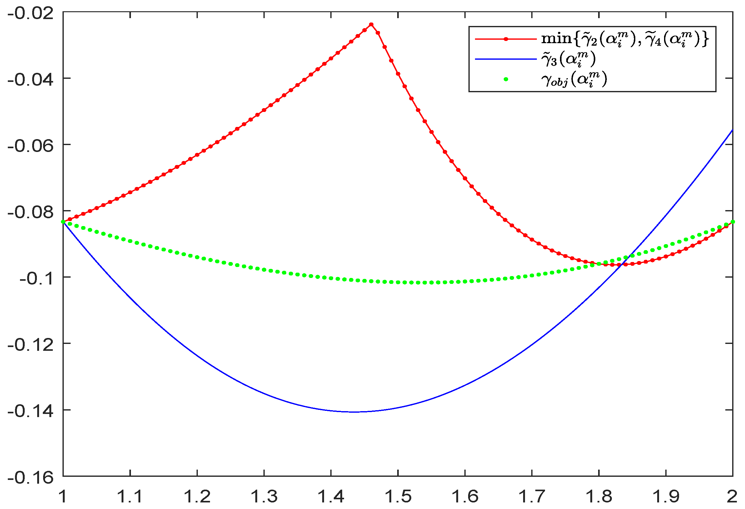
Table 1. The CPU time, the average number of iterations (for PGMRES) and errors of numerical solutions for IE-4WSGD scheme for

α (x, t) = 1.4 + 0.5 e^{- {(x t)}^{2} - 1}

Table 1. The CPU time, the average number of iterations (for PGMRES) and errors of numerical solutions for IE-4WSGD scheme for

α (x, t) = 1.4 + 0.5 e^{- {(x t)}^{2} - 1}

N	M	Error	${rate}_{h}$	GE	$P_{k_{b}}^{m}$	${\tilde{P}}_{k_{b}}^{m}$
$2^{6}$	$2^{2}$	1.6776e-01	–	(–, 0.0216)	(6.00, 0.0369)	(26.00, 0.0394)
$2^{7}$	$2^{6}$	8.6713e-03	4.26	(–, 0.0895)	(3.92, 0.1379)	(13.81, 0.1398)
$2^{8}$	$2^{10}$	5.3568e-04	4.02	(–, 2.3517)	(1.01, 2.3228)	(1.01, 2.2034)
$2^{9}$	$2^{14}$	3.3459e-05	4.00	(–, 175.5498)	(1.00, 156.8173)	(1.00, 149.2442)

Table 2. The CPU time, the average number of iterations (for PGMRES) and errors of numerical solutions for IE-4WSGD scheme for

α (x, t) = \frac{545 - {(x t)}^{4}}{300}

Table 2. The CPU time, the average number of iterations (for PGMRES) and errors of numerical solutions for IE-4WSGD scheme for

α (x, t) = \frac{545 - {(x t)}^{4}}{300}

N	M	Error	${rate}_{h}$	GE	$P_{k_{b}}^{m}$	${\tilde{P}}_{k_{b}}^{m}$
$2^{6}$	$2^{2}$	1.0610e-01	–	(–, 0.0212)	(4.00, 0.0365)	(28.50, 0.0391)
$2^{7}$	$2^{6}$	5.7878e-03	4.20	(–, 0.0918)	(2.94, 0.1334)	(22.73, 0.1488)
$2^{8}$	$2^{10}$	3.5884e-04	4.01	(–, 2.4540)	(1.01, 2.4022)	(1.22, 2.3063)
$2^{9}$	$2^{14}$	2.2415e-05	4.00	(–, 177.6686)	(1.00, 161.0472)	(1.00, 152.0569)

Table 3. The CPU time, the average number of iterations (for PGMRES) and errors of numerical solutions for IE-4WSGD scheme with

α (x, y, t) = 1 + 1.6 e^{- x y / 2}

β (x, y, t) = 1 + sin (π x y / 48)

Table 3. The CPU time, the average number of iterations (for PGMRES) and errors of numerical solutions for IE-4WSGD scheme with

α (x, y, t) = 1 + 1.6 e^{- x y / 2}

β (x, y, t) = 1 + sin (π x y / 48)

N	M	Error	${rate}_{h}$	GE	$P_{k_{b}}^{m}$	${\tilde{P}}_{k_{b}}^{m}$
$2^{3}$	$2^{2}$	1.4136e-01	–	(–, 0.1455)	(7.33, 0.1474)	(6.67, 0.1569)
$2^{4}$	$2^{6}$	7.8665e-03	4.17	(–, 0.2134)	(2.60, 0.2876)	(3.03, 0.3827)
$2^{5}$	$2^{10}$	4.8806e-04	4.01	(–, 126.3812)	(1.05, 11.7302)	(1.10, 13.8425)
$2^{6}$	$2^{14}$	3.0296e-05	4.01	(–, 29107.2033)	(1.00, 748.1152)	(1.02, 753.8003)

Table 4. The CPU time, the average number of iterations (for PGMRES) and errors of numerical solutions for IE-4WSGD scheme with

α (x, y, t) = 1.72 - 0.1 (sin (x) cos (x) - sin (y) cos (y))

β (x, y, t) = 1 + e^{- \frac{x y}{3}} + 0.3 cos (\frac{x y}{32})

Table 4. The CPU time, the average number of iterations (for PGMRES) and errors of numerical solutions for IE-4WSGD scheme with

α (x, y, t) = 1.72 - 0.1 (sin (x) cos (x) - sin (y) cos (y))

β (x, y, t) = 1 + e^{- \frac{x y}{3}} + 0.3 cos (\frac{x y}{32})

N	M	Error	${rate}_{h}$	GE	$P_{k_{b}}^{m}$	${\tilde{P}}_{k_{b}}^{m}$
$2^{3}$	$2^{2}$	1.3983e-01	–	(–, 0.1073)	(16.00, 0.1375)	(16.00, 0.1886)
$2^{4}$	$2^{6}$	7.6815e-03	4.19	(–, 0.2687)	(4.68, 0.4383)	(5.59, 0.4450)
$2^{5}$	$2^{10}$	4.7459e-04	4.02	(–, 139.7812)	(1.09, 13.7007)	(1.17, 12.0109)
$2^{6}$	$2^{14}$	2.9450e-05	4.01	(–, 13772.3810)	(1.02, 1010.3408)	(1.07, 1216.1459)

Table 5. Errors of numerical solutions IE-4WSGD scheme with

α (x, y, t) = 1 + e^{- x y} / e^{t}

β (x, y, t) = 1 + sin (π x y / 48) / e^{t}

Table 5. Errors of numerical solutions IE-4WSGD scheme with

α (x, y, t) = 1 + e^{- x y} / e^{t}

β (x, y, t) = 1 + sin (π x y / 48) / e^{t}

N	M	Error	${rate}_{h}$
$2^{3}$	$2^{2}$	5.6644e-02	–
$2^{4}$	$2^{6}$	6.1470e-03	3.20
$2^{5}$	$2^{10}$	4.0610e-04	3.92
$2^{6}$	$2^{14}$	2.5891e-05	3.97

Table 6. Errors of numerical solutions IE-4WSGD scheme with

α (x, y, t) = 1.72 - 0.1 (sin (x) cos (x t) - sin (y) cos (y t))

β (x, y, t) = 1 + e^{- t} e^{- x y / 11}

Table 6. Errors of numerical solutions IE-4WSGD scheme with

α (x, y, t) = 1.72 - 0.1 (sin (x) cos (x t) - sin (y) cos (y t))

β (x, y, t) = 1 + e^{- t} e^{- x y / 11}

N	M	Error	${rate}_{h}$
$2^{3}$	$2^{2}$	6.7791e-02	–
$2^{4}$	$2^{6}$	3.9463e-03	4.10
$2^{5}$	$2^{10}$	2.5590e-04	3.95
$2^{6}$	$2^{14}$	1.6331e-05	3.97

Disclaimer/Publisher’s Note: The statements, opinions and data contained in all publications are solely those of the individual author(s) and contributor(s) and not of MDPI and/or the editor(s). MDPI and/or the editor(s) disclaim responsibility for any injury to people or property resulting from any ideas, methods, instructions or products referred to in the content.

© 2024 by the authors. Licensee MDPI, Basel, Switzerland. This article is an open access article distributed under the terms and conditions of the Creative Commons Attribution (CC BY) license (http://creativecommons.org/licenses/by/4.0/).

Copyright: This open access article is published under a Creative Commons CC BY 4.0 license, which permit the free download, distribution, and reuse, provided that the author and preprint are cited in any reuse.

MDPI Initiatives

Important Links

Choose an area of interest and we will send you notifications of new preprints at your preferred frequency.

Disclaimer

High Order Difference Schemes for Space Riesz Variable-Order Nonlinear Fractional Diffusion Equations

Abstract

1. Introduction

2. 4WSGD Operators for Riemann-Liouville VO Fractional Derivatives

3. IE-4WSGD Scheme for 1D SRVONFDE

3.1. IE-4WSGD Scheme

3.2. Stability and Convergence Analysis

4. Preconditioning Techniques

5. IE-4WSGD Scheme for 2D SRVONFDE

6. Numerical Results

7. Concluding Remarks

Author Contributions

Funding

Data Availability Statement

Acknowledgments

Conflicts of Interest

References

MDPI Initiatives

Important Links

Subscribe