SOAMC: A Semi-Supervised Open Set RecognitionAlgorithm for Automatic Modulation Classification

1. Introduction

In modern communication systems, different modulation schemes directly impact data transmission performance and spectral efficiency. As such, the accurate identification of modulation modes plays a critical role in signal processing, resource allocation, and overall system optimization. Automatic Modulation Classification (AMC) [1,2,3] represents a significant technological advancement that enables the automatic detection of the modulation scheme used in a received signal. Widely applied in the field of communications, AMC technology is instrumental in optimizing system performance, efficiently allocating resources, and effectively managing the communication spectrum by precisely identifying modulation schemes.

Despite its advancements, the field of AMC continues to encounter significant challenges, including signal noise, multipath fading, and frequency offset, all of which contribute to signal degradation. Furthermore, the increasing diversity and complexity of modulation schemes intensify the difficulty of the classification task. As AMC is inherently a pattern recognition problem, the integration of artificial intelligence (AI) technologies, such as intelligent signal processing [4,5,6], has emerged as a promising solution in electromagnetic signal processing. With ongoing technological advancements, AI has demonstrated substantial potential in improving pattern recognition. In particular, deep learning [7,8], renowned for its ability to automatically extract complex features and enhance recognition accuracy, has been extensively adopted in this field.

In the field of deep learning research on signal modulation classification, the collection of a substantial volume of electromagnetic sample signals is crucial for supervised training. However, this process typically requires considerable human and material resources. The acquisition of radio frequency (RF) signals from the environment involves the use of various spectrum acquisition devices and signal processing techniques to generate visual representations of signals, such as afterglow plots, waterfall plots, and spectrum maps. Signal analysis in this context demands experts to carefully examine the time-frequency characteristics of the signals in order to accurately identify the target signal. This technology necessitates a high level of expertise and technical proficiency from operators. Nevertheless, as the volume of radio signals increases or the monitoring period extends, the efficiency and accuracy of manual analysis significantly decline. To overcome these challenges, semi-supervised learning [9,10] offers a promising solution in modulation signal recognition by reducing the dependence on labeled samples. Through the use of semi-supervised learning algorithms, a large volume of unlabeled modulation signal samples can be leveraged for model training, even when only a limited number of labeled samples are available. This approach significantly reduces the need for labeled data and enhances both the efficiency and accuracy of modulation signal recognition.

With the rapid advancement of communication technology, the need for effective communication signal recognition has become increasingly urgent. In the domain of communication signal classification and recognition, deep learning has achieved significant progress. However, existing methods typically assume that test samples belong to the known categories present in the training set, an assumption that often does not hold true in practical applications. As a result, the challenge of open set recognition (OSR) has gained considerable attention. The objective of OSR is to develop algorithms capable of handling unknown category samples, thereby enhancing the robustness and generalization ability of machine learning systems. Compared to traditional closed-set recognition, OSR presents greater challenges. In an open-set environment, it is impossible to obtain training data that encompasses all possible categories in advance, making it difficult to distinguish unknown category samples from known categories. To address this issue, researchers have proposed a range of innovative methods and techniques, including anomaly detection algorithms, generative models, and metric learning approaches. These methods aim to establish robust decision boundaries that can effectively differentiate between unknown and known category samples.

Open set semi-supervised learning is a crucial and challenging field that aims to address the open set classification problem while maximizing the use of unlabeled data. In traditional supervised learning, training samples from known categories are typically sufficient and reliable, but unknown categories remain unaddressed. In open set classification, however, the presence of both known and unknown category samples introduces significant challenges to conventional supervised learning algorithms. This paper proposes a semi-supervised open set recognition algorithm, SOAMC, specifically designed for automatic modulation classification. The algorithm enhances the robustness of the pre-trained model through data augmentation and adaptive adjustment techniques. Additionally, the proposed open set feature embedding strategy effectively leverages a small amount of labeled data to achieve detailed classification under open set conditions. The algorithm demonstrates excellent performance, particularly in scenarios with limited labeled data. In cases with only five labeled samples per category and per signal-to-noise ratio (SNR), the SOAMC method achieves a 2% accuracy improvement over the FreeMatch method. Moreover, when the number of labeled samples increases to 10 and 20 per category and per SNR, the SOAMC algorithm outperforms FreeMatch, with accuracy improvements of 4% and 3%, respectively. These results strongly demonstrate that the proposed SOAMC method outperforms FreeMatch in scenarios with scarce labeled data, proving its efficacy in open set semi-supervised learning.

In summary, we have made the following three main contributions:

• We propose a semi-supervised open-set modulation recognition algorithm called SOAMC, which performs label propagation on a large number of unlabeled samples. This approach effectively addresses the challenge of automatic modulation classification and recognition in open environments, relying only on a small number of labeled samples
• We design an adaptive enhancement module that leverages data augmentation and adaptive modulation techniques to significantly enhance the robustness of the pre-trained model. Experimental results demonstrate that this module effectively improves the model’s recognition accuracy, even when only a small number of labeled samples are available.
• We propose an open-set feature embedding strategy that effectively utilizes a minimal number of labeled samples to achieve accurate classification in open-set modulation recognition. The effectiveness of the proposed algorithm is validated through simulation experiments.

The following introduces the general content of each section of this article. In Section 2, related work is elaborated. In Section 3, we introduce SOAMC, a semi-supervised open-set modulation recognition algorithm, and describe the proposed method in detail. The simulation results are presented in Section 4, while Section 5 provides a summary of the conclusions.

2. Related Work

2.1. Semi-Supervised Learning

Semi-supervised learning (SSL) is a machine learning approach that lies between the supervised and unsupervised learning paradigms. It leverages a small set of labeled data alongside a large amount of unlabeled data for pattern recognition [11,12].The primary goal of SSL is to overcome the limitations of supervised and unsupervised methods by enabling the model to autonomously leverage unlabeled samples and improve performance without external intervention.

A prominent research focus in semi-supervised learning is pseudo-labeling [13]. In [14], Zou et al. introduced the Confidence Regularized Self-Training (CRST) method, which treats pseudo-labels as continuous hidden variables and iteratively refines them through optimization. The approach employs two regularization techniques. The first, label regularization, enhances the entropy of pseudo-labels during the labeling process, similar to label smoothing. The second, model regularization (MR), increases the entropy of network output probabilities during network retraining. The experimental results presented by the authors confirm the effectiveness of confidence regularization. Specifically, when the pseudo-label matches the true label, both regularization strategies slightly reduce the probability of the corresponding class for the pseudo-label. Conversely, when the pseudo-label does not match the true label, the probability of the corresponding class for the pseudo-label is significantly reduced.

In [15], Mukherjee et al. introduced the concept of Bayesian inconsistent active learning for assessing the uncertainty of sample labels. They utilized this uncertainty to choose pseudo-labeled samples for model retraining, aiming to bolster the reliability of pseudo-labels and mitigate the influence of noise. Through the incorporation of extra unlabeled samples, a larger dataset is made available for model training, thereby enhancing generalization performance. Furthermore, by eliminating the noise from unlabeled data, the model’s robustness and performance can be enhanced. In [16], the FixMatch method was introduced by Sohn et al. The core concept of FixMatch involves aligning the predictions of strongly augmented unlabeled data with the pseudo-labels of weakly augmented data when the model’s confidence in the weakly augmented data is high. This process aims to improve the model training. FixMatch has demonstrated notable effectiveness in scenarios with limited labeled data. Despite the proliferation of research on pseudo-label learning techniques in recent years and the advancements in semi-supervised learning, existing approaches often rely on predefined static thresholds or proprietary threshold adjustment strategies. These methods are not universally applicable to diverse signal samples and neural network architectures, thereby constraining the progress of deep learning in the domain of modulation recognition.

2.2. Data Augmentation

Data augmentation enhances the robustness of deep neural networks. In [17], RandAugment was introduced, offering a significant reduction in the search space by discovering a generalizable augmentation strategy across various datasets. This method employs two interpretable hyperparameters to control the augmentation intensity, tailored to specific tasks and datasets. The interpretability of these parameters allows for deeper exploration of the types and roles of augmentations applied to diverse models and datasets. The efficacy of RandAugment has been validated, particularly in the context of semi-supervised image classification tasks. In another investigation [18], the Unsupervised Data Augmentation (UDA) technique was introduced. The algorithm involves initially applying a back-translation data method, followed by a semi-supervised data augmentation approach for classification, leading to enhanced classification accuracy. To incorporate unlabeled data into the classification model, the study utilizes KL (Kullback-Leibler) divergence to assess the objective function of the unlabeled data.

2.3. Automatic Modulation Classification Utilizing Deep Learning

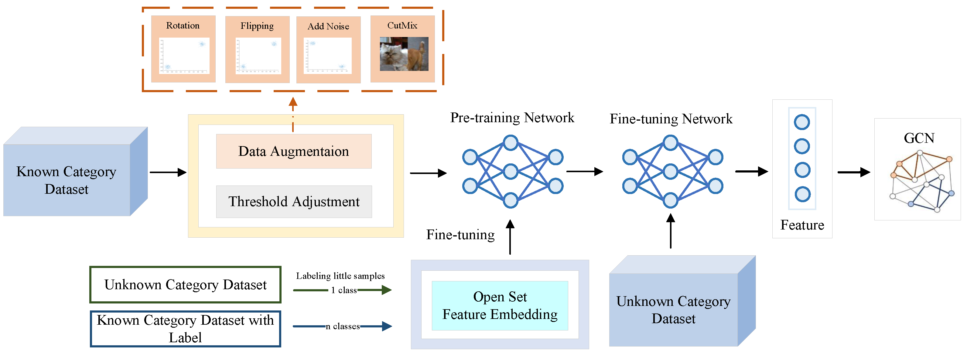
With the rapid advancement of technology, deep learning [8,19,20,21,22,23,24,25,26,27] has become a formidable tool across a wide range of disciplines. Its applications span various sectors, including education, healthcare [28], and other domains of everyday life, encompassing areas such as computer vision [29], speech recognition [30], natural language processing, and finance. However, the integration of deep learning technology within the field of wireless communications remains in its early stages.

Significant advancements in image recognition, driven by the development of deep neural networks, have sparked interest in their application for automatic modulation classification. O’Shea et al. [31,32,33] explored the integration of deep learning into radio communication and identification, proposing an automatic modulation classification technique utilizing Convolutional Neural Networks (CNNs). This method leverages the time-domain representation of radio signals as input, enabling automatic feature extraction through convolutional layers, followed by classification via fully connected layers. The training and testing datasets were generated using GnuRadio, encompassing 11 modulation schemes. Zhang et al. [34] introduced a novel approach that combines deep CNN and long short-term memory (LSTM) models, accompanied by a signal preprocessing technique that integrates in-phase, quadrature, and fourth-order statistical characteristics. This method led to an 8% performance improvement of the CNN-LSTM models on the test dataset. Zheng et al. [35] proposed three fusion techniques: voting-based, confidence-based, and feature-based fusion, demonstrating through simulations that these methods outperform non-fusion approaches. Additionally, Chen et al. [36] developed a novel attention collaboration framework aimed at enhancing the accuracy of automatic modulation recognition (AMC) using deep learning. Experiments on the RML2016.10a dataset revealed that the proposed framework outperforms other deep learning models, including VGG, GoogleNet, and ResNet.

In general, deep learning-based automatic modulation classification methods have achieved substantial performance improvements in modulation classification tasks. Unlike traditional feature-based approaches, deep learning methods automatically learn feature representations and exhibit superior generalization capabilities. However, these methods typically require large volumes of labeled data for training, and their design and tuning demand specialized expertise and experience. Given the challenges in acquiring labeled data in practice, this paper investigates a semi-supervised signal recognition approach that aims to label a large quantity of unlabeled samples using only a small number of labeled samples.

3. Method

This section provides an introduction to the semi-supervised open set modulation recognition proach,with a detailed description of the specific structure and training methods of each component of the proposed SOAMC. The adaptive enhancement module uses modulated signal flipping, rotation, noise addition, and CutMix algorithms for data enhancement, and incorporates adaptive adjustment of confidence thresholds to improve the performance of pre-trained modulated signal recognition networks. The open set features are embedded in the fine tuning network, which is used to extract features and feed them into the graph neural network for label propagation. It is capable of refine classification of unknown samples in cases where the unknown samples are very few by manual labeling. The structure of SOAMC is shown in Figure 1.

3.1. Adaptive Enhancement Module

The adaptive augmentation module combines the advantages of data augmentation and threshold adjustment to improve the performance of the pre-trained network for modulated signal recognition. The complete module algorithm is provided in Algorithm 1.

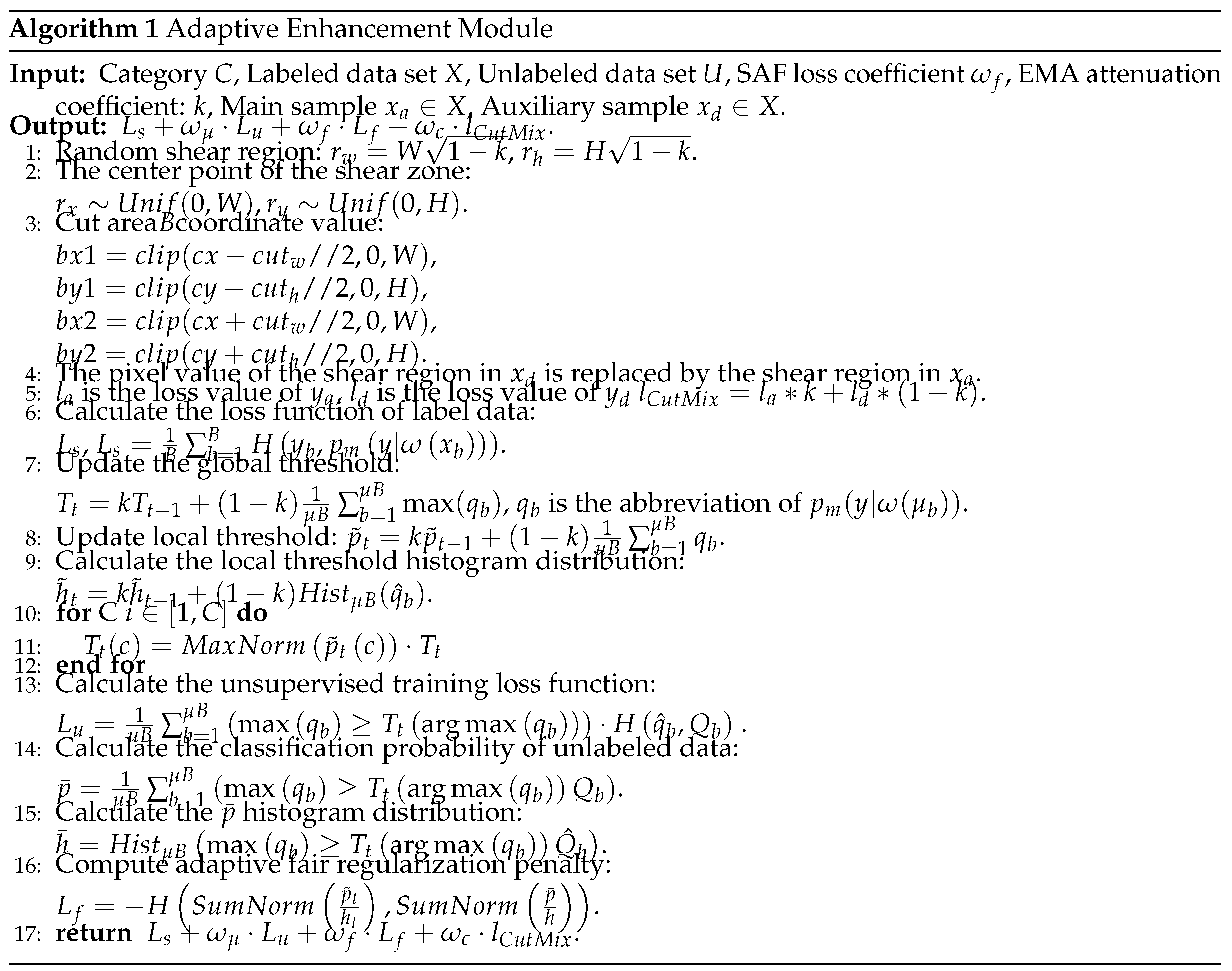
3.1.1. Data Augmentation

Data augmentation is a commonly employed technique in deep learning as it enhances the model’s generalization capabilities and mitigates overfitting. The principal data augmentation techniques utilized in this module include rotation, flipping, Gaussian noise, and CutMix data augmentation.

The method of data rotation for the original I/Q signal significantly differs from that in the field of images. In image processing, rotation typically involves the clockwise or counterclockwise rotation of a two-dimensional image based on intuitive perception. However, in electromagnetic signal processing, the rotation operation entails mapping the I/Q data to the complex domain. Subsequently, based on the distribution pattern of sample points in the complex domain, a clockwise or counterclockwise rotation is executed around the origin to enhance the rotation effect of the I/Q data in the complex domain. This complex operation aims to better address the characteristics of electromagnetic signals, distinguishing it from the rotation method used in image processing. By utilizing the formula 1, the modulated wireless signal $\left(I,Q\right)$ is rotated at different angles around its origin to derive the enhanced signal sample $\left(I^{\prime },Q^{\prime }\right)$.

$$\left[\begin{array}{c}{I}^{\prime }\\ Q^{\prime }\end{array}\right]=\left[\begin{array}{cc}cos\theta & -sin\theta \\ sin\theta & cos\theta \end{array}\right]\left[\begin{array}{c}I\\ Q\end{array}\right].$$

(1)

Complex domain flipping and complex domain rotation encounter analogous challenges. In the realm of image processing, the direct application of the flip operation to electromagnetic signals is impeded due to its inability to alter data within the complex space. Consequently, to attain the desired flip enhancement effect, it becomes imperative to initially map the signal’s sample points to the complex space before executing the flip operation. For a provided modulated wireless signal $\left(I,Q\right)$, a horizontal flip is delineated by interchanging the I value with its opposite. The precise computational procedure is outlined as follows:

$$\left[\begin{array}{c}{I}^{\prime }\\ Q^{\prime }\end{array}\right]=\left[\begin{array}{c}-I\\ Q\end{array}\right],$$

(2)

The vertical flip operation involves changing the Q value to its opposite, which can be computed as follows:

$$\left[\begin{array}{c}{I}^{\prime }\\ Q^{\prime }\end{array}\right]=\left[\begin{array}{c}I\\ -Q\end{array}\right].$$

(3)

By introducing Gaussian noise $N\left(0,{\sigma }^2\right)$ to the modulated wireless signal $\left(I,Q\right)$, an improved signal sample $\left(I^{\prime },Q^{\prime }\right)$ is generated. The detailed computational procedure is outlined as follows:

$$\left[\begin{array}{c}{I}^{\prime }\\ Q^{\prime }\end{array}\right]=\left[\begin{array}{c}I\\ Q\end{array}\right]+N\left(0,{\sigma }^2\right).$$

(4)

Among these, ${\sigma }^2$ represents the noise variance. Through the selection of a sufficient number of distinct $\sigma$ values, Gaussian noise data augmentation has the potential to substantially increase the size of the dataset.

CutMix is a data augmentation technique utilized to improve the resilience and generalization capacity of the model. This method generates novel training instances by blending local regions from different samples. Specifically, CutMix involves extracting a segment from the original image and randomly incorporating pixel values from other samples in the training dataset into this region, distributing the classification outcomes based on a specific ratio. This procedure aids in eliminating irrelevant pixels during training, thus enhancing training efficiency.

$x_a$ and $x_b$ represent distinct training samples, while $y_a$ and $y_b$ denote their respective labeled values. In the context of CutMix, the objective is to create a novel training sample along with its associated labels: $\tilde{x}$ and $\tilde{y}$.

$$\tilde{x}=M\odot x_a+\left(1-M\right)\odot x_b,$$

(5)

$$\tilde{y}=k{y}_a+(1-k)y_b.$$

(6)

$M\in {\left\{0,1\right\}}^{H\times W}$ represent a binary mask used for dropping out parts of a region and for padding. The symbol ⊙ denotes pixel-by-pixel multiplication. The binary mask 1 consists of all elements being 1. The parameter k follows a Beta distribution similar to Mixup.

If k follows a Beta distribution with parameters $\alpha$ and $\alpha$, where $\alpha =1$, then k follows a uniform distribution on the interval (0, 1).

To sample the binary mask, the bounding box of the clipping region $B=\left(r_x,r_y,r_w,r_h\right)$ is initially sampled. This bounding box is then utilized for the indicative calibration of the clipping region for the samples $x_a$ and $x_b$. The formula for sampling the bounding box of the clipping region is as follows:

$$r_x\sim Unif(0,W),r_w=W\sqrt{1-k},$$

(7)

$$r_y\sim Unif(0,H),r_h=H\sqrt{1-k}.$$

(8)

3.1.2. Threshold Adjustment

The threshold adjustment comprises two main components: Self-Adaptive Thresholding (SAT) and Self-Adaptive Class Fairness Regularization (SAF). SAT is responsible for maintaining the quality of pseudo-tags by dynamically modifying the threshold, whereas SAF promotes diverse predictions by employing Class Fairness Regularization.

Adaptive thresholding can be specifically categorized into adaptive global thresholding and adaptive local thresholding. The global threshold is determined based on the average confidence of the model in unlabeled data, however, due to the huge amount of unlabeled data, calculating the confidence for all the unlabeled data at each time step or training period can be time consuming. Therefore, the exponential moving average (EMA) technique is used to approximate the global confidence level, which is calculated as follows:

$$T_t=\left\{\begin{array}{c}{\displaystyle \frac{1}{C}},\\ k{T}_{t-1}+(1-k){\displaystyle \frac{1}{\mu B}}{\sum }_{b=1}^{\mu B}max\left(q_b\right),\end{array}\begin{array}{c}t=0\\ other\end{array}\right.$$

(9)

Here, T denotes the global threshold and t denotes the time step iteration. Specifically, the variable T is initialized to ${\displaystyle \frac{1}{C}}$, where C denotes the number of categories. Where $X=\left\{(x_b,y_b):b\in (1,2,...,B)\right\}$ represents a labeled data set, $U=\left\{u_b:b\in (1,2,\dots ,\mu B)\right\}$ is unlabeled dataset. $k\in (0,1)$ is the momentum decay of EMA.

Adaptive local thresholding computes the expectation of the model’s predictions for each category c to estimate category-specific learning states. The computational formula is as follows:

$${\tilde{p}}_t\left(c\right)=\left\{\begin{array}{c}{\displaystyle \frac{1}{C}},\\ k{\tilde{p}}_{t-1}\left(c\right)+(1-k){\displaystyle \frac{1}{\mu B}}{\sum }_{b=1}^{\mu B}{q}_b\left(c\right),\end{array}\begin{array}{c}t=0\\ other\end{array}\right.$$

(10)

Here, ${\tilde{p}}_t=\left[{\tilde{p}}_t\left(1\right),{\tilde{p}}_t\left(2\right),...,{\tilde{p}}_t\left(C\right)\right]$ is a list containing all ${\tilde{p}}_t\left(c\right)$.

The final threshold is adaptively adjusted by integrating the global and local thresholds to obtain the final adaptive threshold $T_t\left(c\right)$:

$$T_t\left(c\right)=MaxNorm\left({\tilde{p}}_t\left(c\right)\right)·T_t.$$

(11)

where $MaxNorm$ denotes the maximum normalization, specifically:

$$x^{\prime }={\displaystyle \frac{x}{max\left(x\right)}}.$$

(12)

Finally, the unsupervised training target $L_u$ at the t-th iteration is:

$$L_u={\displaystyle \frac{1}{\mu B}}\sum _{b=1}^{\mu B}max\left(q_b\right)>T_t(argmax\left(q_b\right))·H({\widehat{q}}_b,Q_b).$$

(13)

where $H(·)$ represents the cross-entropy loss function.

Because real-world scenarios often do not satisfy the class balance condition, instead of penalizing the model with the class-averaged prior that has often been used before, the sliding average EMA from the model prediction ${\tilde{p}}_t$ is used here as the expected predictive distribution of the estimated unlabeled data. Considering that the distribution of potential pseudo-labels may be uneven, the fairness objective is moderated in an adaptive manner, i.e., the expectation of the probability is normalized by the histogram distribution of the pseudo-labels to counteract the negative effect of imbalance. The formula is calculated as follows:

$$\overline{p}={\displaystyle \frac{1}{\mu B}}\sum _{b=1}^{\mu B}I(max\left(q_b\right)\ge T_t(argmax\left(q_b\right))Q_b,$$

(14)

$$\overline{h}=His{t}_{\mu B}\left(I(max\left(q_b\right)\ge T_t(argmax\left(q_b\right)){\widehat{Q}}_b\right).$$

(15)

Similar to the calculation of ${\tilde{p}}_t$, the value of ${\tilde{h}}_t$ is determined as follows:

$${\tilde{h}}_t=k{\tilde{h}}_{t-1}+(1-k)His{t}_{\mu B}\left({\widehat{q}}_b\right).$$

(16)

The adaptive fair regularization penalty $L_f$ at step t is defined as follows:

$$L_f=-H\left(SumNorm\left({\displaystyle \frac{{\tilde{p}}_t}{{\tilde{h}}_t}}\right),SumNorm\left({\displaystyle \frac{\overline{p}}{\overline{h}}}\right)\right).$$

(17)

The training objective of the final model consists of the cross-entropy of labeled data, the unsupervised training loss function $L_u$, and the adaptive fair regularization penalty $L_f$

3.2. Open Set Feature Embedding

Open-set feature embedding acquires signals of known classes and a small number of labeled incremental class signals, intercepting the convolutional structure of the pretrained model to fine-tune the new feature extractor. Consider that the feature extractor obtained by intercepting the pre-trained model on the known class has limited or even no feature extraction capability for incremental class signals. In order to fully utilize the pre-trained model on the known and a large number of unlabeled incremental class signals, the feature extractor is designed in a certain way. A moderate amount of all unlabeled incremental signals are treated as one class (without differentiation) and allowed to be learned by the pre-trained model to obtain rough supervised information about these incremental classes. Based on this, the newly obtained pre-trained model is fine-tuned to obtain a new feature extractor.

3.3. Graph Neural Network

The goal of graph semi-supervised learning is to process data with a graph structure where only a small number of nodes are labeled and most of them are unlabeled. The task is to predict the labels of the unlabeled nodes. Therefore, the graph semi-supervised learning algorithm is suitable for the case where only a small number of samples are labeled. The SOAMC method employs graph semi-supervised learning to label the unlabeled samples. A small number of labeled samples and a large number of unlabeled samples are constructed as a similarity graph, the nodes represent the samples, and the edges of the graph represent the degree of similarity between the two samples. Finally labeling of unlabeled samples is achieved using label propagation algorithm.

4. Experiment

4.1. Simulation Verification

4.1.1. Simulation Setup

In order to validate the ability of the proposed SOAMC method for signal recognition identification with a limited number of labeled samples, a simulation dataset is constructed for testing. The dataset setup is shown in Table 1.

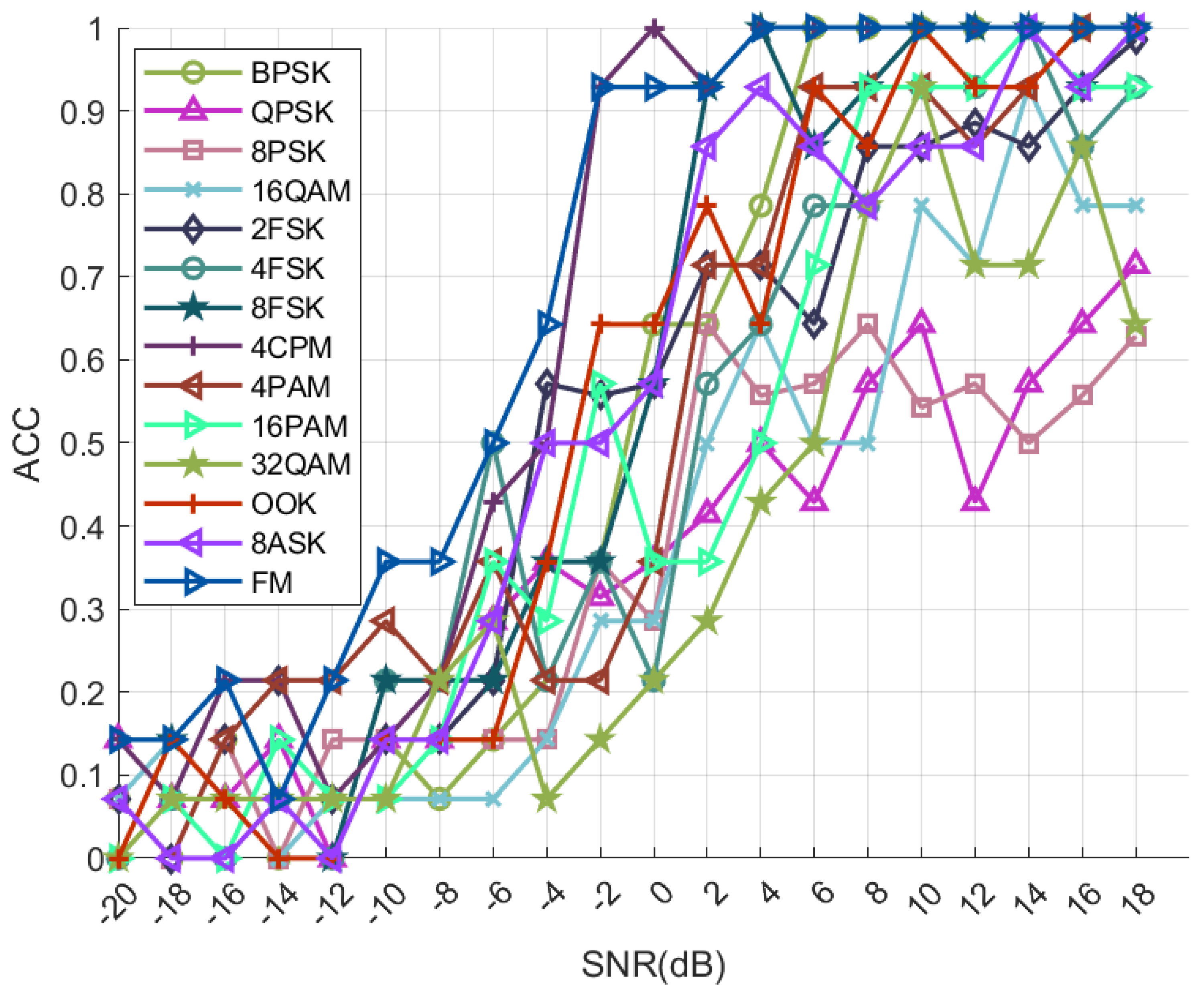
4.1.2. Simulation Results

Our proposed semi-supervised open set identification algorithm SOAMC, which relies on only a small amount of manual labeling, is capable of refine classification of unknown samples. The experimental results are shown in Figure 2, and the simulation results show that the recognition rates of the added classes OOK, 8ASK and FM can reach 99% at 18 dB.

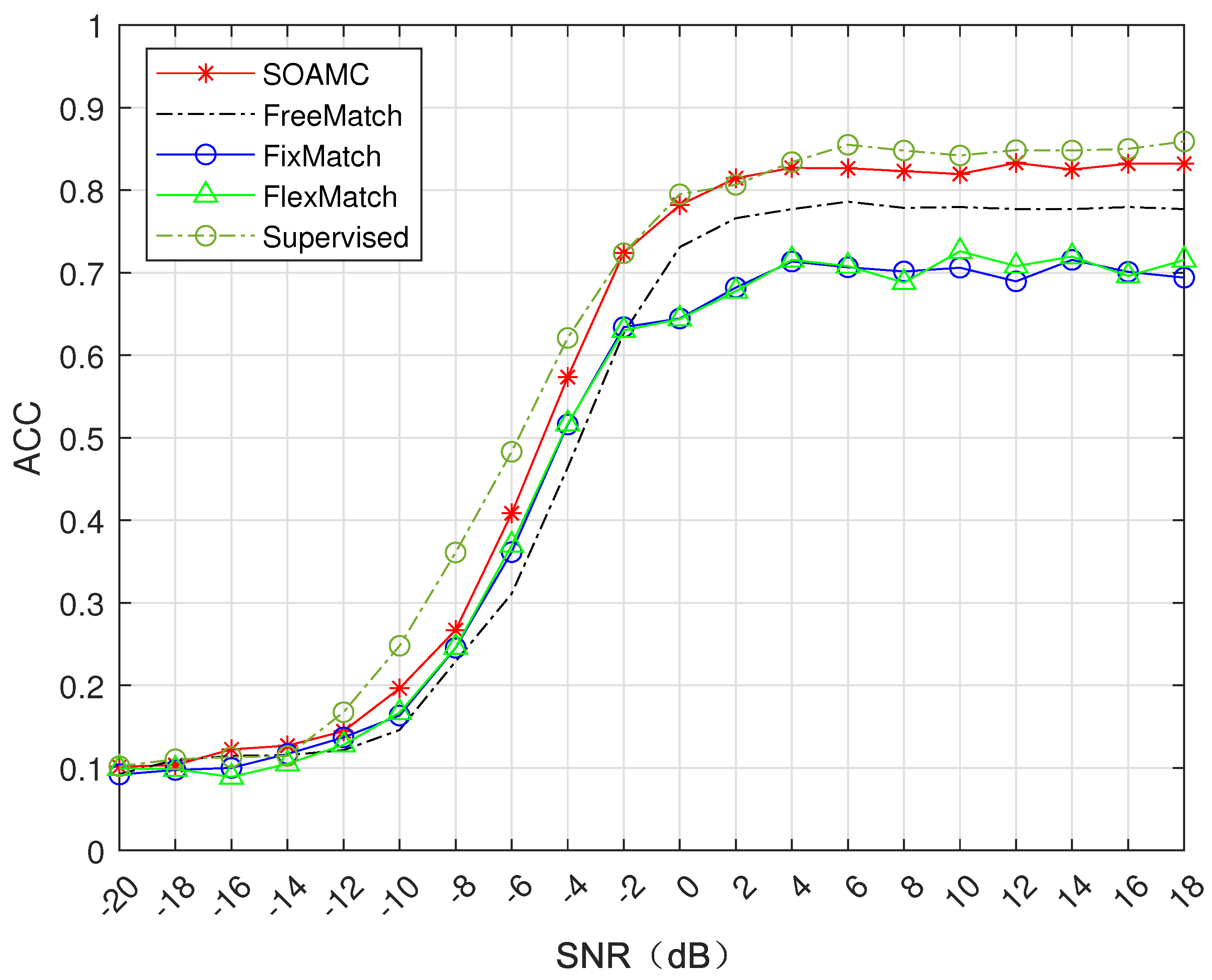
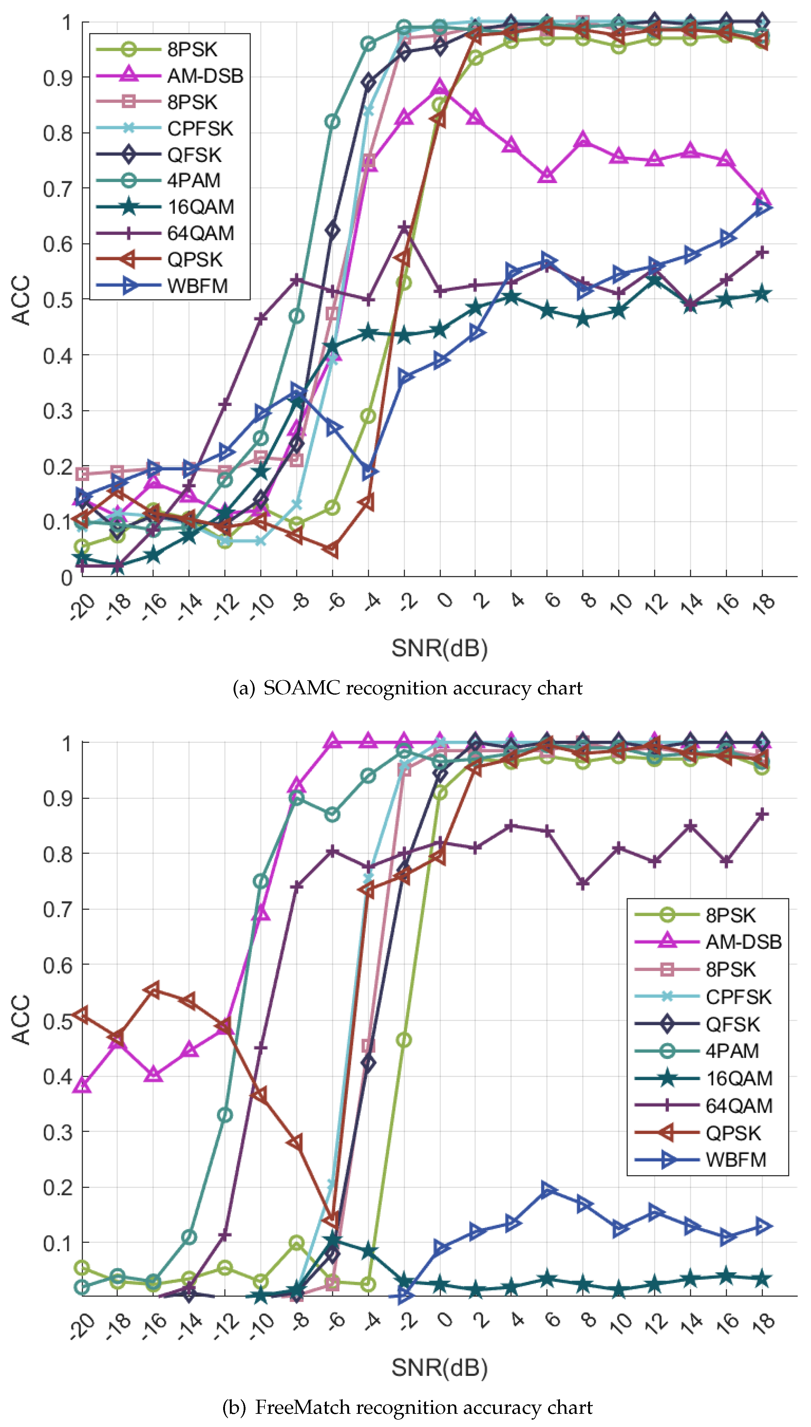
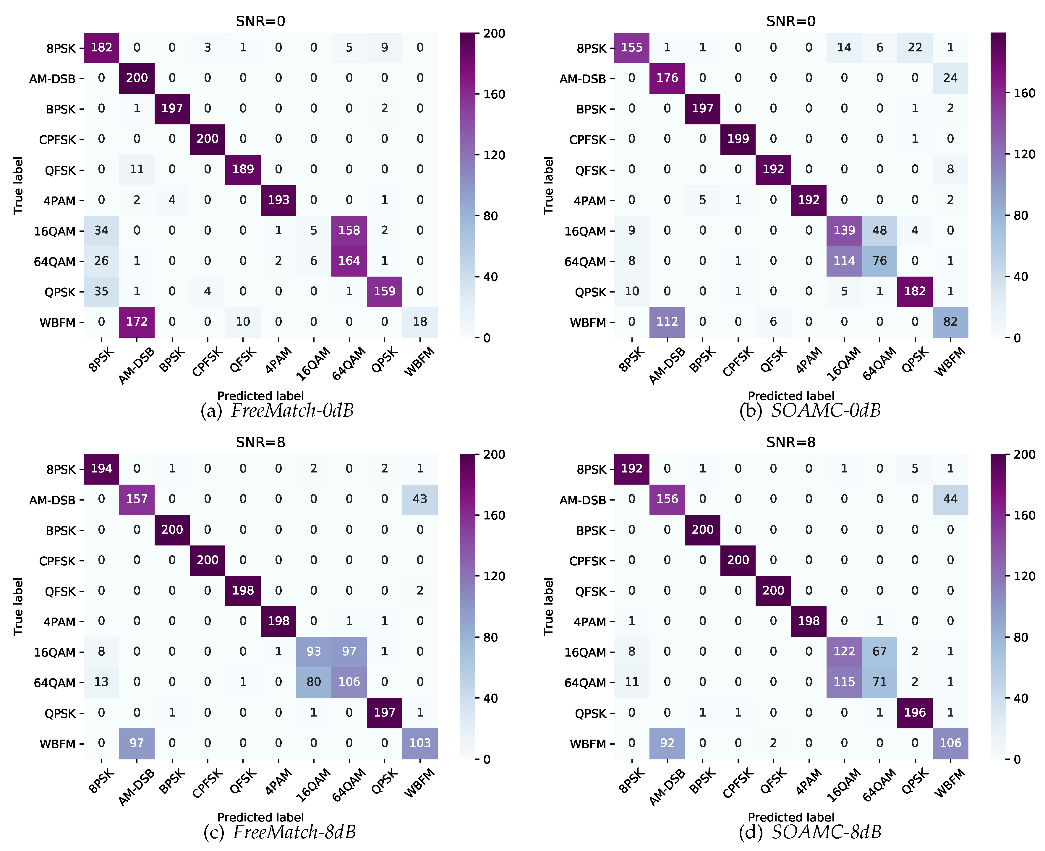
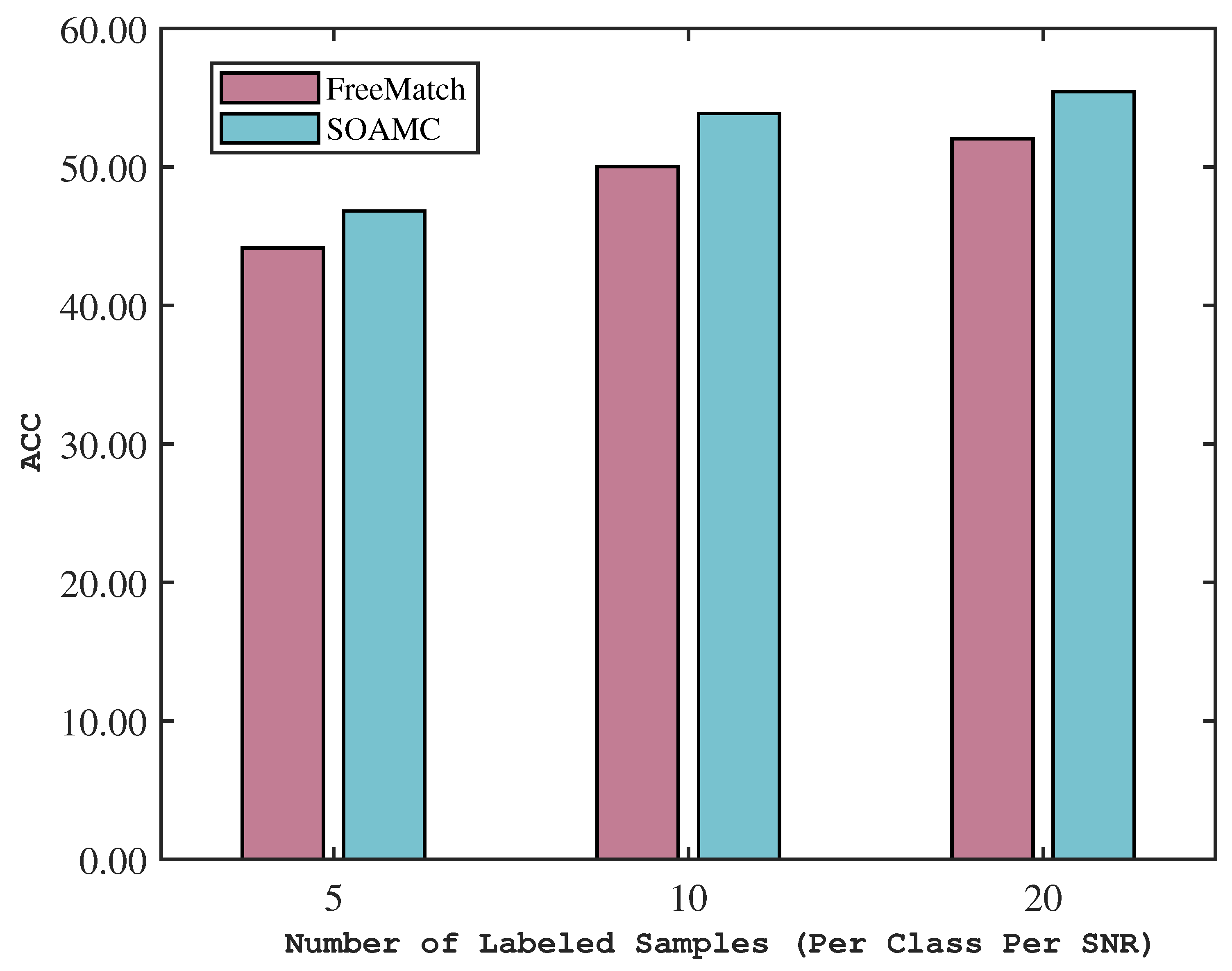
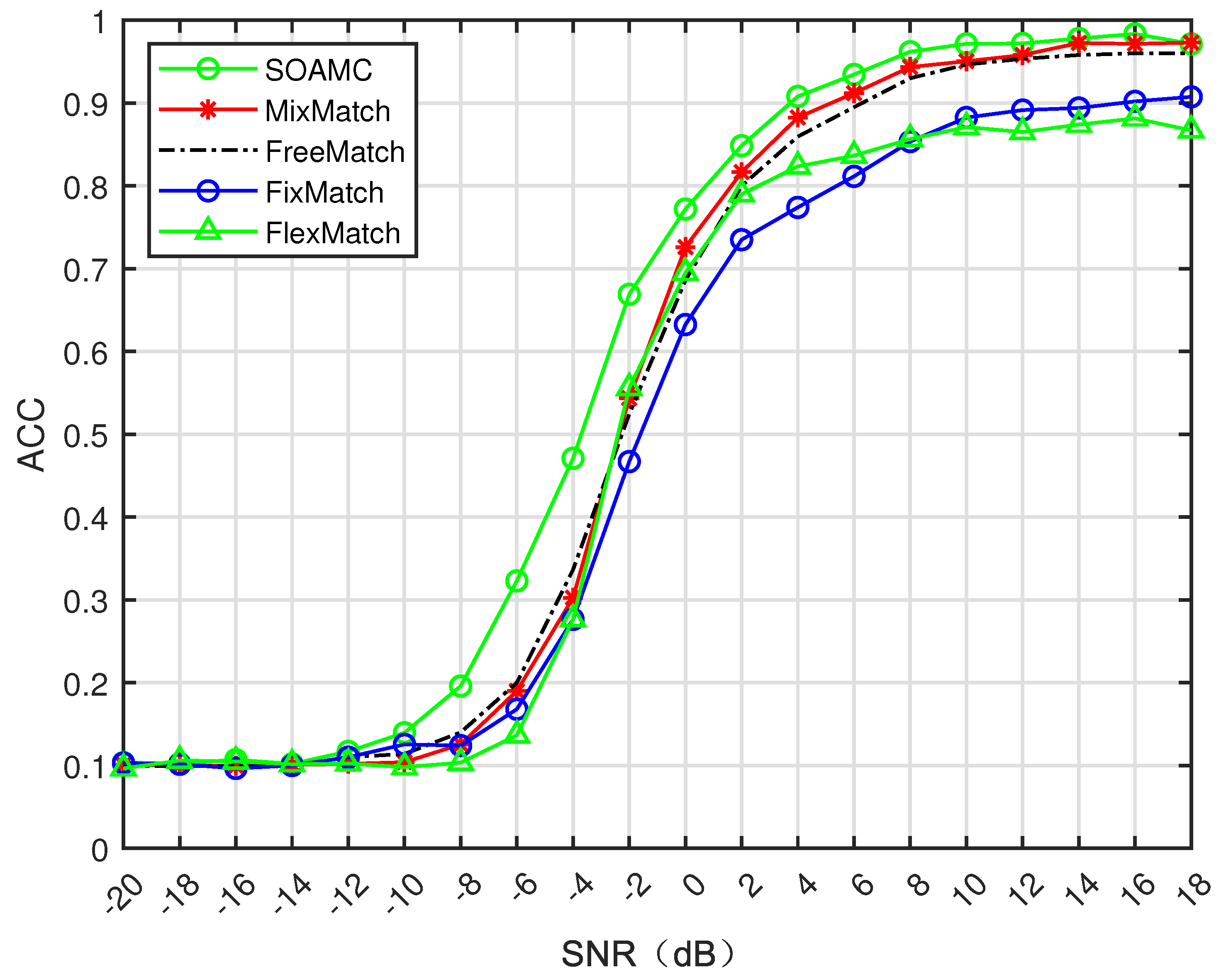
4.2. Comparative Experiment

In order to validate the effectiveness of the proposed SOAMC algorithm, validation has been carried out using publicly available datasets and homemade datasets, respectively, and comparative experiments have been conducted with existing methods.

4.2.1. Public Dataset Validation

The validation of this experiment was conducted using the RML2016.10a public dataset. In their study, Javier Maroto et al. [37] identified the issue of AM-SSB signals being obscured by AWGN noise, leading to the deliberate exclusion of AM-SSB signals from the experimental dataset. The dataset comprises ten modulation types, including 8PSK, AM-DSB, BPSK, CPFSK, QFSK, 4PAM, 16QAM, 64QAM, QPSK, and WBFM, encompassing a range of 20 signal-to-noise ratios from -20 dB to 18 dB.

The convergence curves for the fully supervised learning, FlexMatch algorithm [38], FixMatch algorithm [16], FreeMatch algorithm [39], and the SOAMC algorithm proposed in this study are illustrated in Figure 3. These curves depict the training process of the model for the test set of the recognition accuracy convergence curve. The model is trained for semi-supervised learning using data composition that includes 20 labeled data per class per SNR, 1,000 unlabeled data per class per SNR, and 200 test data per class per SNR. In contrast, fully-supervised learning employs 1,000 labeled data per class per SNR for training.

It can be seen from Figure 3 that the recognition accuracy of FlexMatch algorithm and FixMatch algorithm is low, especially after 0dB, FlexMatch algorithm and FixMatch algorithm show a lower recognition rate. The recognition rate of FreeMatch algorithm is higher than that of FlexMatch algorithm and FixMatch algorithm. It can be seen that FreeMatch adaptive threshold adjustment and adaptive fair regularization multiplication are effective for modulated signal data. The accuracy of the proposed SOAMC algorithm in low SNR and high SNR is significantly higher than that of the FreeMatch algorithm, and it is close to the fully supervised algorithm, which shows the effectiveness of the proposed SOAMC algorithm.

Figure 4a,b depict the recognition accuracy of each modulation mode at various signal-to-noise ratios. A comparison of the two figures reveals that SOAMC demonstrates significant enhancements for the challenging modulation types of WBFM and 16QAM.

The analysis of the confusion matrices presented in Figure 5a,b reveals that the model trained using the FreeMatch algorithm exhibits notably low WBFM recognition accuracy at 0dB. Specifically, a significant portion of WBFMs are misclassified as AM-DSBs, while a majority of 16QAMs are misclassified as 64QAMs. This deficiency in accurately recognizing WBFMs and 16QAMs primarily contributes to the overall poor performance of the FreeMatch algorithm at 0dB. Conversely, the model trained with the SOAMC algorithm demonstrates substantial enhancements in the recognition accuracy of WBFM and 16QAM signals at 0dB. This improvement underscores the efficacy of the optimization scheme proposed in this study, which in turn validates the superiority of the enhanced algorithm introduced herein.

The confusion matrix depicted in Figure 5c,d illustrates that the model trained using the FreeMatch algorithm did not exhibit any enhancement in the recognition accuracy of WBFM and 16QAM signals at 8dB and 0dB, as shown in Figure 5a,b. Specifically, a significant portion of WBFM signals were misclassified as AM-DSB, while a considerable number of 16QAM signals were misidentified as 64QAM. This misclassification of WBFM and 16QAM signals primarily contributed to the overall poor recognition accuracy of the FreeMatch algorithm at 10dB. In contrast, the model trained with the SOAMC algorithm demonstrated notable improvements in the recognition accuracy of WBFM and 16QAM signals at 10dB. A comparison between Figures 5a,b indicates a substantial increase in the recognition rate of WBFM signals at 10dB compared to 0dB. This observation validates that the optimization strategy proposed in this study facilitates an enhanced recognition rate at higher signal-to-noise ratios, aligning more closely with the characteristics of modulated signal data. Consequently, this study affirms the efficacy of the algorithm proposed herein for processing modulated signals.

Figure 6 illustrates a comparison of the recognition rates between FreeMatch and the proposed SOAMC algorithm across varying numbers of labeled samples. When faced with severely limited labeled data, specifically 5 labeled samples per class per signal-to-noise ratio, the SOAMC method demonstrates a 2% increase in accuracy compared to the FreeMatch approach. Moreover, with only 10 and 20 labeled samples per class per SNR, the SOAMC algorithm exhibits enhanced recognition performance, showcasing accuracy improvements of 4% and 3% over the FreeMatch method, respectively. These results unequivocally establish the superior performance of the proposed method over the FreeMatch technique in scenarios with scarce labeled data.

4.2.2. Self-Made Data Set Verification

The accuracy curves depicting the recognition performance of the model on the test set during the training phase of the SOAMC, MixMatch, FreeMatch, FixMatch, and FlexMatch algorithms introduced in this study are illustrated in Figure 7. The training dataset utilized in the model training consists of 30 labeled data instances per class per signal-to-noise ratio, 1000 unlabeled data instances per class per signal-to-noise ratio, and 200 test data instances per class per signal-to-noise ratio, with data distributed across ten classes. Analysis of Figure 7 reveals that the recognition accuracy curves of the FixMatch and FlexMatch algorithms exhibit lower accuracy levels compared to other algorithms. Notably, the SOAMC algorithm consistently outperforms the FreeMatch algorithm across all signal-to-noise ratios, indicating the efficacy of the proposed approach.

5. Conclusions

This paper presents an in-depth analysis of the current development trends and challenges in automatic modulation classification technologies, particularly in open-set scenarios. To address the limitations of existing open-set modulation recognition techniques, we propose a semi-supervised open-set recognition method, SOAMC. By incorporating data augmentation and adaptive adjustment techniques in the pre-training phase, the algorithm enhances its robustness. Furthermore, the designed open-set feature embedding mechanism refines the classification of unknown samples, even in cases where only a limited number of samples are manually labeled. Simulation experiments conducted on both open-source and self-constructed datasets demonstrate the effectiveness of the proposed SOAMC method, highlighting its potential for practical application in open-set modulation recognition.

With the rapid advancement of deep learning technologies, the modulation recognition of communication signals has become increasingly intelligent, fostering the integration of communication systems and deep learning. This convergence has attracted considerable attention and presents new opportunities for further exploration. In light of the research focus and objectives of this study, several promising areas for future research are identified:

• This paper presents a novel approach to open-set recognition and semi-supervised modulation signal classification, aiming to improve the accuracy of classifying known samples while developing robust rejection mechanisms for samples from unknown classes. However, the subsequent processing and interpretability of rejected samples remain underexplored. Future work could benefit from a deeper investigation into extending open-set recognition tasks by incorporating new class discovery techniques, which would enhance the system’s ability to manage previously unseen modulation types.
• Furthermore, while the proposed method demonstrates strong performance when a small number of unknown category samples are manually labeled, exploring alternative approaches to identify unknown data without relying on manual labeling is a compelling avenue for future research. This would involve developing fully automated mechanisms to recognize unknown categories, expanding the applicability of the method in more dynamic and real-time communication environments.

References

1. Dobre, O.A.; Abdi, A.; Bar-Ness, Y.; Su, W. Survey of automatic modulation classification techniques: Classical approaches and new trends. IET communications 2007, 1, 137–156. [Google Scholar] [CrossRef]
2. Xu, J.L.; Su, W.; Zhou, M. Likelihood-ratio approaches to automatic modulation classification. IEEE Transactions on Systems, Man, and Cybernetics, Part C (Applications and Reviews) 2010, 41, 455–469. [Google Scholar] [CrossRef]
3. Zhang, Z.; Wang, C.; Gan, C.; Sun, S.; Wang, M. Automatic modulation classification using convolutional neural network with features fusion of SPWVD and BJD. IEEE Transactions on Signal and Information Processing over Networks 2019, 5, 469–478. [Google Scholar] [CrossRef]
4. Zheng, S.; Hu, J.; Zhang, L.; Qiu, K.; Chen, J.; Qi, P.; Zhao, Z.; Yang, X. FM-Based Positioning via Deep Learning. IEEE Journal on Selected Areas in Communications, 2024; 1. [Google Scholar] [CrossRef]
5. Zheng, S.; Yang, Z.; Shen, F.W.; Zhang, L.; Zhu, J.; Zhao, Z.; Yang, X. Deep Learning-Based DOA Estimation. IEEE Transactions on Cognitive Communications and Networking 2024, 10, 819–835. [Google Scholar] [CrossRef]
6. Qi, P.; Jiang, T.; Xu, J.; He, J.; Zheng, S.; Li, Z. Unsupervised Spectrum Anomaly Detection With Distillation and Memory Enhanced Autoencoders. IEEE Internet of Things Journal. [CrossRef]
7. Goodfellow, I.; Bengio, Y.; Courville, A. Deep learning; MIT press, 2016.
8. LeCun, Y.; Bengio, Y.; Hinton, G. Deep learning. nature 2015, 521, 436–444. [Google Scholar] [CrossRef] [PubMed]
9. Van Engelen, J.E.; Hoos, H.H. A survey on semi-supervised learning. Machine learning 2020, 109, 373–440. [Google Scholar]
10. Zhou, Z.H.; Zhou, Z.H. Semi-supervised learning. Machine Learning, 2021; 315–341. [Google Scholar]
11. Wang, H.; Zhang, Q.; Wu, J.; Pan, S.; Chen, Y. Time series feature learning with labeled and unlabeled data. Pattern Recognition 2019, 89, 55–66. [Google Scholar] [CrossRef]
12. Simao, M.; Mendes, N.; Gibaru, O.; Neto, P. A review on electromyography decoding and pattern recognition for human-machine interaction. Ieee Access 2019, 7, 39564–39582. [Google Scholar] [CrossRef]
13. Pseudo-Label, D.H.L. The simple and efficient semi-supervised learning method for deep neural networks. In Proceedings of the ICML 2013 Workshop: Challenges in Representation Learning; 2013; pp. 1–6. [Google Scholar]
14. Zou, Y.; Yu, Z.; Liu, X.; Kumar, B.; Wang, J. Confidence regularized self-training. In Proceedings of the Proceedings of the IEEE/CVF international conference on computer vision, 2019, pp. 5982–5991.
15. Mukherjee, S.; Awadallah, A.H. Uncertainty-aware self-training for text classification with few labels. arXiv preprint arXiv:2006.15315, 2020; arXiv:2006.15315 2020. [Google Scholar]
16. Sohn, K.; Berthelot, D.; Carlini, N.; Zhang, Z.; Zhang, H.; Raffel, C.A.; Cubuk, E.D.; Kurakin, A.; Li, C.L. Fixmatch: Simplifying semi-supervised learning with consistency and confidence. Advances in neural information processing systems 2020, 33, 596–608. [Google Scholar]
17. Cubuk, E.D.; Zoph, B.; Shlens, J.; Le, Q.V. Randaugment: Practical automated data augmentation with a reduced search space. In Proceedings of the Proceedings of the IEEE/CVF conference on computer vision and pattern recognition workshops, 2020, pp. 702–703.
18. Xie, Q.; Dai, Z.; Hovy, E.; Luong, T.; Le, Q. Unsupervised data augmentation for consistency training. Advances in neural information processing systems 2020, 33, 6256–6268. [Google Scholar]
19. Deng, L.; Yu, D.; et al. Deep learning: Methods and applications. Foundations and trends® in signal processing 2014, 7, 197–387. [Google Scholar] [CrossRef]
20. He, K.; Zhang, X.; Ren, S.; Sun, J. Deep residual learning for image recognition. In Proceedings of the Proceedings of the IEEE conference on computer vision and pattern recognition, 2016, pp. 770–778.
21. Zhang, C.; Bengio, S.; Hardt, M.; Recht, B.; Vinyals, O. Understanding deep learning (still) requires rethinking generalization. Communications of the ACM 2021, 64, 107–115. [Google Scholar] [CrossRef]
22. Gui, G.; Huang, H.; Song, Y.; Sari, H. Deep learning for an effective nonorthogonal multiple access scheme. IEEE Transactions on Vehicular Technology 2018, 67, 8440–8450. [Google Scholar] [CrossRef]
23. Zhang, Y.; Doshi, A.; Liston, R.; Tan, W.t.; Zhu, X.; Andrews, J.G.; Heath, R.W. DeepWiPHY: Deep learning-based receiver design and dataset for IEEE 802.11 ax systems. IEEE Transactions on Wireless Communications 2020, 20, 1596–1611. [Google Scholar]
24. Ghasemzadeh, P.; Banerjee, S.; Hempel, M.; Sharif, H. A novel deep learning and polar transformation framework for an adaptive automatic modulation classification. IEEE Transactions on Vehicular Technology 2020, 69, 13243–13258. [Google Scholar] [CrossRef]
25. Lyu, Z.; Wang, Y.; Li, W.; Guo, L.; Yang, J.; Sun, J.; Liu, M.; Gui, G. Robust automatic modulation classification based on convolutional and recurrent fusion network. Physical Communication 2020, 43, 101213. [Google Scholar] [CrossRef]
26. Weng, L.; He, Y.; Peng, J.; Zheng, J.; Li, X. Deep cascading network architecture for robust automatic modulation classification. Neurocomputing 2021, 455, 308–324. [Google Scholar] [CrossRef]
27. Zhang, H.; Nie, R.; Lin, M.; Wu, R.; Xian, G.; Gong, X.; Yu, Q.; Luo, R. A deep learning based algorithm with multi-level feature extraction for automatic modulation recognition. Wireless Networks 2021, 27, 4665–4676. [Google Scholar]
28. Shang, J.; Sun, Y. Predicting the hosts of prokaryotic viruses using GCN-based semi-supervised learning. BMC biology 2021, 19, 1–15. [Google Scholar] [CrossRef]
29. Han, H.; Ma, W.; Zhou, M.; Guo, Q.; Abusorrah, A. A novel semi-supervised learning approach to pedestrian reidentification. IEEE Internet of Things Journal 2020, 8, 3042–3052. [Google Scholar] [CrossRef]
30. Khonglah, B.; Madikeri, S.; Dey, S.; Bourlard, H.; Motlicek, P.; Billa, J. Incremental semi-supervised learning for multi-genre speech recognition. In Proceedings of the ICASSP 2020-2020 IEEE International Conference on Acoustics, Speech and Signal Processing (ICASSP). IEEE, 2020, pp. 7419–7423.
31. O’Shea, T.J.; Corgan, J.; Clancy, T.C. Unsupervised representation learning of structured radio communication signals. In Proceedings of the 2016 First International Workshop on Sensing, Processing and Learning for Intelligent Machines (SPLINE). IEEE, 2016, pp. 1–5.
32. O’Shea, T.J.; West, N.; Vondal, M.; Clancy, T.C. Semi-supervised radio signal identification. In Proceedings of the 2017 19th International Conference on Advanced Communication Technology (ICACT). IEEE, 2017, pp. 33–38.
33. O’shea, T.J.; West, N. Radio machine learning dataset generation with gnu radio. In Proceedings of the Proceedings of the GNU Radio Conference. 2016, 1, number 1. [Google Scholar]
34. Zhang, M.; Zeng, Y.; Han, Z.; Gong, Y. Automatic modulation recognition using deep learning architectures. In Proceedings of the 2018 IEEE 19th International Workshop on Signal Processing Advances in Wireless Communications (SPAWC). IEEE, 2018, pp. 1–5.
35. Zheng, S.; Qi, P.; Chen, S.; Yang, X. Fusion methods for CNN-based automatic modulation classification. IEEE Access 2019, 7, 66496–66504. [Google Scholar] [CrossRef]
36. Chen, S.; Zhang, Y.; He, Z.; Nie, J.; Zhang, W. A novel attention cooperative framework for automatic modulation recognition. IEEE Access 2020, 8, 15673–15686. [Google Scholar] [CrossRef]
37. Huynh-The, T.; Pham, Q.V.; Nguyen, T.V.; Nguyen, T.T.; Ruby, R.; Zeng, M.; Kim, D.S. Automatic modulation classification: A deep architecture survey. IEEE Access 2021, 9, 142950–142971. [Google Scholar]
38. Zhang, B.; Wang, Y.; Hou, W.; Wu, H.; Wang, J.; Okumura, M.; Shinozaki, T. Flexmatch: Boosting semi-supervised learning with curriculum pseudo labeling. Advances in Neural Information Processing Systems 2021, 34, 18408–18419. [Google Scholar]
39. Wang, Y.; Chen, H.; Heng, Q.; Hou, W.; Fan, Y.; Wu, Z.; Wang, J.; Savvides, M.; Shinozaki, T.; Raj, B.; et al. Freematch: Self-adaptive thresholding for semi-supervised learning. arXiv preprint arXiv:2205.07246, 2022; arXiv:2205.07246 2022. [Google Scholar]
Figure 1. The structure of SOAMC framework. The adaptive enhancement module utilizes data enhancement and threshold adjustment techniques to pre-train signal feature extraction networks. Open-set features are embedded in the pre-training network, then features are extracted using the fine-tuning network, and features are fed into a graph neural network for label propagation.
Preprints 119412 g001
Figure 2. Recognition accuracy of SOAMC algorithm in open set scenarios.
Preprints 119412 g002
Figure 3. Accuracy comparison chart under 20 labeled data for each class and SNR.
Preprints 119412 g003
Figure 4. Recognition accuracy of each modulation at each SNR, SOAMC has a performance improvement over FreeMatch.
Preprints 119412 g004
Figure 5. Comparison of results between SOAMC and FreeMatch split on 0dB and 8dB on the confusion matrix.
Preprints 119412 g005
Figure 6. Comparison of recognition accuracy of different number of labeled data.
Preprints 119412 g006
Figure 7. Recognition accuracy curves of SOAMC, MixMatch, FreeMatch, FixMatch and FlexMatch for the test set of the model during training.
Preprints 119412 g007