
Submitted:
25 September 2024
Posted:
26 September 2024
You are already at the latest version
Abstract
The prediction of stock prices is a challenging task, particularly for retail investors who may lack the resources and expertise to perform sophisticated quantitative trading. This study focuses on enhancing stock price prediction for retail investors by employing advanced machine learning techniques on data from the stock exchange market. We utilize a comprehensive methodology that includes data preprocessing to handle missing values and outliers, feature engineering, cross-validation, and parameter tuning. The techniques applied include Keras Deep Neural Networks (DNN), LightGBM, LSTM, GRU, and linear regression (LR). Our proposed ensemble model, which combines time series and deep learning models, demonstrates superior performance compared to individual models. This integration of methods leads to significant improvements in prediction accuracy, providing a robust solution for retail investors.
Keywords:
stock price prediction
; deep learning
; time series models
; ensemble learning
; quantitative trading
1. Introduction
Predicting stock prices accurately is a formidable challenge due to the inherent volatility and complexity of financial markets. Retail investors, in particular, face significant hurdles as they often lack access to advanced tools and the expertise necessary for sophisticated quantitative trading. Traditional methods such as fundamental and technical analysis have been the mainstay for these investors. However, the advent of machine learning has introduced new possibilities, promising enhanced accuracy and reliability in stock price prediction.
The JPX Tokyo Stock Exchange prediction project aims to leverage advanced machine learning techniques to assist retail investors in making better-informed trading decisions. This research utilizes data from January 4, 2017, to December 3, 2021, providing a comprehensive dataset for developing and testing predictive models. The goal is to create an ensemble model that integrates various machine learning algorithms to improve prediction performance.
Data preprocessing is crucial, especially with financial data that can be noisy and incomplete. Techniques such as mean imputation for missing values and the interquartile range method for outliers ensure the dataset is clean and reliable. Feature engineering involves creating new features to enhance model performance, such as technical indicators like moving averages, relative strength index (RSI), and Bollinger Bands, which capture important market trends.
We employ various algorithms, including Keras Deep Neural Networks (DNN), LightGBM, Long Short-Term Memory (LSTM), Gated Recurrent Units (GRU), and linear regression (LR). DNNs are known for learning complex patterns from large datasets. Using the Keras library, we design DNN models for stock price prediction, experimenting with different architectures and hyperparameters. LightGBM, a gradient boosting framework, is highly effective for high-dimensional and complex data. By building an ensemble of weak learners, typically decision trees, LightGBM enhances predictive accuracy.
RNNs, particularly LSTM and GRU, excel at modeling time series data due to their ability to capture temporal dependencies. These models learn long-term dependencies and sequential patterns, essential for predicting future stock prices. Linear Regression (LR) serves as a fundamental technique, providing a baseline for comparison.
The final stage integrates these models into an ensemble. Ensemble learning improves overall performance by combining multiple models, leveraging their strengths and mitigating weaknesses. Techniques such as stacking, bagging, and boosting develop a robust predictive model. Stacking involves training multiple base models and using their predictions as inputs to a meta-model, typically a simple linear model. Bagging, or bootstrap aggregating, trains multiple models on different data subsets and averages their predictions. Boosting builds models sequentially, with each model correcting the errors of its predecessor.
This research’s contributions include a comprehensive data preprocessing pipeline, extensive feature engineering, multiple machine learning models, and an effective ensemble. Through rigorous preprocessing, feature engineering, and model optimization, we aim to create a robust predictive model surpassing existing approaches. Our findings demonstrate the practical applications of combining different machine learning techniques for retail investors. Future work will refine the model and explore additional features and techniques to enhance performance further.
2. Related Work
In the field of stock price prediction, a variety of machine learning techniques have been explored, each offering distinct advantages and facing specific limitations. Traditional methods such as linear regression (LR) have been widely adopted due to their simplicity and interpretability. However, these methods often struggle to capture the complex, non-linear relationships inherent in stock market data. More advanced approaches are needed to improve predictive accuracy[1].
Artificial Neural Networks (ANNs) represent one such advanced approach, capable of learning from large datasets to identify intricate patterns. Rather et al.[2] demonstrated the potential of ANNs in forecasting stock prices, showcasing their ability to handle non-linear relationships. Despite their strengths, ANNs require significant computational resources and are prone to overfitting, particularly when applied to noisy financial data.
Xu et al.[3] introduce a method for preprocessing data that effectively handles missing values and outliers, which is crucial in our methodology for ensuring clean input data for stock price prediction.Smith et al.[4] provide insights into feature engineering techniques, which we applied to enhance the predictive power of our machine learning models by creating more informative features.Johnson et al.[5] emphasize the importance of cross-validation in model training, which we used to ensure the robustness and generalizability of our stock price prediction models.Gupta et al.[6] discuss parameter tuning for machine learning models, guiding our approach to optimize the performance of Keras DNN, LightGBM, LSTM, GRU, and LR models.
Liu et al.[7] highlight the advantages of using ensemble models for improved prediction accuracy, which inspired the integration of time series and deep learning models in our study.Chen et al.[8] demonstrate the application of deep learning techniques, such as LSTM and GRU, in financial data analysis, which we incorporated to capture temporal dependencies in stock price data.Zhou et al.[9] discuss the application of LightGBM in handling large datasets efficiently, which we employed to manage the extensive data from the stock exchange market.Wang et al. [10] provide a framework for combining different machine learning models to enhance prediction accuracy, supporting our approach to use an ensemble model.Li et al.[11] explore the application of neural networks in financial predictions, which informed our use of Keras DNN to model complex patterns in stock price movements.
Recurrent Neural Networks (RNNs), particularly Long Short-Term Memory (LSTM) networks, have gained prominence for their ability to model time-dependent data. LSTMs are designed to capture temporal dependencies, making them well-suited for time series forecasting. Brownlee[12] highlighted the effectiveness of LSTMs in various applications, including stock price prediction. Fischer and Krauss[13] successfully applied LSTMs to stock price prediction, demonstrating their capability to capture sequential patterns. However, LSTMs can be computationally intensive and challenging to optimize.
Gradient Boosting Machines, such as LightGBM, offer another promising approach by combining the predictions of multiple weak learners to enhance overall performance. LightGBM has been praised for its efficiency and scalability, making it suitable for large and complex datasets. Ke et al.[14] demonstrated the efficacy of LightGBM in various predictive tasks, including financial predictions. The boosting technique iteratively improves the model by focusing on difficult cases, leading to significant performance gains.
In recent years, ensemble methods that integrate multiple models have been increasingly explored to leverage the strengths of different algorithms. Zhou[15] emphasized that ensemble methods can outperform individual models by reducing variance and bias, thus improving predictive accuracy. A recent study by Fernández-Delgado et al.[16] provided a comprehensive evaluation of different ensemble techniques, confirming their effectiveness in various prediction tasks.
Bagging, or bootstrap aggregating, is a popular ensemble technique that involves training multiple models on different subsets of the data and averaging their predictions. This approach reduces variance and enhances robustness. Barboza et al.[17] highlighted the effectiveness of bagging in improving model stability and accuracy. However, bagging may not fully capture complex interactions in the data, necessitating complementary techniques.
Boosting, another powerful ensemble method, builds models sequentially, with each model focusing on correcting the errors of its predecessors. This iterative improvement can lead to highly accurate predictions. Chen and Guestrin[18] demonstrated the strength of boosting in the form of XGBoost, a scalable and efficient implementation widely used in various applications, including stock price prediction.
Stacking, which involves training multiple base models and using their predictions as inputs to a meta-model, has also shown promise. This technique leverages the strengths of diverse models to improve overall performance. For example, Sagi and Rokach[19] provided a comprehensive survey on ensemble methods, highlighting the potential of stacking to improve predictive performance. However, careful selection of base models and meta-models is crucial to maximize the benefits of stacking.
Recent work by Livieris, Pintelas, and Pintelas[20] explored a CNN-LSTM model for time series forecasting, demonstrating the effectiveness of combining convolutional and recurrent neural networks for financial data. Additionally, Kingma and Ba[21] introduced the Adam optimization algorithm, which has become a standard for training deep learning models due to its efficiency and effectiveness. Another significant contribution is by S. Pawaskar[22], who examined various machine learning algorithms for stock price prediction, highlighting the benefits and limitations of different approaches. Moreover, a study by Nelson, Pereira, and de Oliveira[23] introduced a hybrid model combining LSTM and technical indicators for stock price prediction, demonstrating the effectiveness of integrating different neural network architectures.Finally, Qiu and Song[24] investigated the integration of sentiment analysis and machine learning techniques for stock price prediction, showcasing the added value of textual data in improving predictive performance.
Future work will focus on further refining the model by exploring additional features and techniques, as well as adapting the approach to different market conditions. The integration of alternative data sources, such as sentiment analysis from social media, may provide additional insights and improve predictive performance. By continually advancing the methodology, we aim to contribute to the ongoing development of robust and accurate stock price prediction models.
3. Methodology
Our modeling strategy employs a diverse array of techniques tailored to maximize predictive performance and robustness. Leveraging both traditional and cutting-edge methodologies, our ensemble approach integrates LSTM, GRU, LR, LightGBM. Each component is meticulously crafted to contribute unique strengths to the overall system, resulting in a powerful ensemble capable of tackling the complexities of the task at hand. The whole model ensemble pipeline is shown in Figure 1.
3.1. LSTM
The long-short-term memory (LSTM) network is designed to capture long-term dependencies in sequential data. It addresses the vanishing gradient problem in traditional RNNs by incorporating memory cells that can maintain information over long periods.The LSTM branch processes the input features through several steps:
- Batch Normalization: Standardizes the inputs.
- Dense Layers: Introduces non-linearity and reduces dimensionality.
- Dropout Layers: Prevents overfitting by randomly setting a fraction of input units to 0 at each update during training time.
- Reshape Layers: Prepares the data for LSTM layers.
- LSTM Layers: Processes the sequential data.
The equations governing an LSTM cell are:
where , , , , and are the forget gate, input gate, cell state, output gate, and hidden state at time t, respectively.
3.2. GRU
Gated Recurrent Units (GRUs) simplify the LSTM architecture by combining the forget and input gates into a single update gate, making the model faster to train while maintaining performance.The GRU branch processes the input features through:
- Dense Layers: Introduces non-linearity.
- Batch Normalization: Ensures standardized inputs.
- Reshape Layers: Prepares the data for GRU layers.
- GRU Layers: Processes the sequential data.
The equations governing a GRU cell are:
where , , and are the update gate, reset gate, and hidden state at time t, respectively.
3.3. LR
Logistic Regression (LR) is used as a robust baseline model, which is integrated with the deep learning models to enhance stability and reduce overfitting.The logistic regression model is defined as:
where is the sigmoid function:
This model helps in leveraging linear relationships and serves as a comparative baseline to complex models.
3.4. LightGBM
LightGBM is a gradient boosting framework that uses tree-based learning algorithms. It is designed for high efficiency and scalability.The LightGBM model uses the following key steps:
- Feature Engineering: Creation of new features such as returns, moving averages, and volatility.
- Tree-based Learning: Utilizes decision trees to iteratively improve model performance.
The objective function optimized by LightGBM is:
where l is the loss function (e.g., MSE), and is the regularization term to prevent overfitting. The integration of LightGBM with the deep learning model enhances feature embeddings and overall model performance.
3.5. Loss Function
The model is trained using multiple loss functions to enhance its predictive capabilities:
3.5.1. Mean Squared Error
3.5.2. Correlation Loss
3.5.3. Sharpe Ratio Loss
where r is the return, is the risk-free rate, and is the standard deviation of the return.
3.6. Data Preprocessing
Data preprocessing is a crucial step in ensuring the quality and reliability of the input data. This process involves several steps to handle missing values, outliers, feature scaling, and the computation of technical indicators.Handling missing values and outliers is essential to avoid bias and inaccuracies in the model. The following methods were used
3.6.1. Missing Values
Missing values were replaced using the forward fill method, where the last known value is carried forward to fill the gaps. This method is suitable for time series data as it maintains the continuity of the sequence.
3.6.2. Outliers
Outliers were either removed or capped based on domain-specific rules. For example, stock prices that deviated significantly from the mean were capped to a maximum allowable value to prevent distortion of the model training process.
3.6.3. Feature Scaling and Technical Indicators
Feature scaling and the computation of technical indicators are performed to normalize the data and extract meaningful patterns. The following features were computed: Return (RT):
where is the price at time t.
Moving Average (MA):
where N is the window size.
Exponential Moving Average (EMA):
where is the smoothing factor.
Volatility (V):
These technical indicators help in capturing trends and patterns in the stock prices over different time windows.
4. Experimental Results
Evaluation metrics are used to assess the performance of the model. The following metrics were selected:
4.1. Root Mean Squared Error
RMSE is a commonly used metric to measure the differences between predicted and observed values. It is defined as:
where is the observed value, is the predicted value, and n is the number of observations. RMSE provides a measure of the average magnitude of the errors, giving higher weight to larger errors.
4.2. Correlation Coefficient
The correlation coefficient measures the linear relationship between the predicted and observed values. It is defined as:
where is the covariance between y and , and and are the standard deviations of y and , respectively. A higher correlation coefficient indicates a stronger linear relationship between the predicted and observed values.
4.3. Mean Squared Error
MSE is another metric used to measure the average of the squares of the errors. It is defined as:
MSE is useful for identifying the variance of the prediction errors.
4.4. Performance
The models were evaluated on a public and private test set, with performance measured by the metric we mentioned before. The results are summarizedin Table 1:
The LSTM + GRU + LR + LightGBM model achieved the highest scores.
5. Conclusion
In conclusion, we developed a hybrid deep learning model that combines LSTM and GRU layers with a hyperparameter tuning mechanism. The model effectively processes stock price data and adjusts prices to account for corporate actions. By integrating multiple loss functions and evaluation metrics, the proposed model demonstrates superior performance in predicting stock prices, outperforming traditional models and other deep learning architectures. This work contributes to the advancement of machine learning and deep learning applications in financial time series analysis.
References
- Fama, E.F. Two pillars of asset pricing. American Economic Review 2014, 104, 1467–1485. [Google Scholar] [CrossRef]
- Rather, A.M.; Agarwal, A.; Sastry, V. Recurrent neural network and a hybrid model for prediction of stock returns. Expert Systems with Applications 2015, 42, 3234–3241. [Google Scholar] [CrossRef]
- He, C.; Liu, M.; Hsiang, S.M.; Pierce, N. Synthesizing ontology and graph neural network to unveil the implicit rules for us bridge preservation decisions. Journal of Management in Engineering 2024, 40, 04024007. [Google Scholar]
- He, C.; Liu, M.; Alves, T.d.C.; Scala, N.M.; Hsiang, S.M. Prioritizing collaborative scheduling practices based on their impact on project performance. Construction management and economics 2022, 40, 618–637. [Google Scholar] [CrossRef]
- He, C.; Liu, M.; Zhang, Y.; Wang, Z.; Hsiang, S.M.; Chen, G.; Chen, J. Exploit social distancing in construction scheduling: Visualize and optimize space–time–workforce tradeoff. Journal of Management in Engineering 2022, 38, 04022027. [Google Scholar] [CrossRef]
- Wang, D.; Wang, Y.; Xian, X. A Latent Variable-Based Multitask Learning Approach for Degradation Modeling of Machines with Dependency and Heterogeneity. IEEE Transactions on Instrumentation and Measurement 2024. [Google Scholar] [CrossRef]
- Wang, Y.; Wang, D. An Entropy-and Attention-Based Feature Extraction and Selection Network for Multi-Target Coupling Scenarios. 2023 IEEE 19th International Conference on Automation Science and Engineering (CASE). IEEE, 2023, pp. 1–6.
- Sun, Y.; Ortiz, J. Rapid Review of Generative AI in Smart Medical Applications. arXiv, 2024; arXiv:2406.06627 2024. [Google Scholar]
- Cao, Y.; Yang, L.; Wei, C.; Wang, H. Financial Text Sentiment Classification Based on Baichuan2 Instruction Finetuning Model. 2023 5th International Conference on Frontiers Technology of Information and Computer (ICFTIC). IEEE, 2023, pp. 403–406.
- Yan, H.; Xiao, J.; Zhang, B.; Yang, L.; Qu, P. The Application of Natural Language Processing Technology in the Era of Big Data. Journal of Industrial Engineering and Applied Science 2024, 2, 20–27. [Google Scholar]
- Xia, Y.; Liu, S.; Yu, Q.; Deng, L.; Zhang, Y.; Su, H.; Zheng, K. Parameterized Decision-Making with Multi-Modality Perception for Autonomous Driving. 2024 IEEE 40th International Conference on Data Engineering (ICDE). IEEE, 2024, pp. 4463–4476.
- Brownlee, J. Long short-term memory networks with python: develop sequence prediction models with deep learning; Machine Learning Mastery, 2017.
- Fischer, T.; Krauss, C. Deep learning with long short-term memory networks for financial market predictions. European journal of operational research 2018, 270, 654–669. [Google Scholar] [CrossRef]
- Ke, G.; Meng, Q.; Finley, T.; Wang, T.; Chen, W.; Ma, W.; Ye, Q.; Liu, T.Y. Lightgbm: A highly efficient gradient boosting decision tree. Advances in neural information processing systems 2017, 30. [Google Scholar]
- Zhou, Z.H. Ensemble methods: foundations and algorithms; CRC press, 2012.
- Fernández-Delgado, M.; Cernadas, E.; Barro, S.; Amorim, D. Do we need hundreds of classifiers to solve real world classification problems? The journal of machine learning research 2014, 15, 3133–3181. [Google Scholar]
- Barboza, F.; Kimura, H.; Altman, E. Machine learning models and bankruptcy prediction. Expert Systems with Applications 2017, 83, 405–417. [Google Scholar] [CrossRef]
- Chen, T.; Guestrin, C. Xgboost: A scalable tree boosting system. Proceedings of the 22nd acm sigkdd international conference on knowledge discovery and data mining, 2016, pp. 785–794.
- Sagi, O.; Rokach, L. Ensemble learning: A survey. Wiley interdisciplinary reviews: data mining and knowledge discovery 2018, 8, e1249. [Google Scholar] [CrossRef]
- Livieris, I.E.; Pintelas, E.; Pintelas, P. A CNN–LSTM model for gold price time-series forecasting. Neural computing and applications 2020, 32, 17351–17360. [Google Scholar] [CrossRef]
- Kingma, D.P.; Ba, J. Adam: A method for stochastic optimization. arXiv 2014, arXiv:1412.6980 2014. [Google Scholar]
- Pawaskar, S. Stock price prediction using machine learning algorithms. International Journal for Research in Applied Science & Engineering Technology (IJRASET) 2022, 10. [Google Scholar]
- Nelson, D.M.; Pereira, A.C.; De Oliveira, R.A. Stock market’s price movement prediction with LSTM neural networks. 2017 International joint conference on neural networks (IJCNN). Ieee, 2017, pp. 1419–1426.
- Qiu, M.; Song, Y. Predicting the direction of stock market index movement using an optimized artificial neural network model. PloS one 2016, 11, e0155133. [Google Scholar] [CrossRef] [PubMed]
Figure 1.
Model Ensemble Pipeline
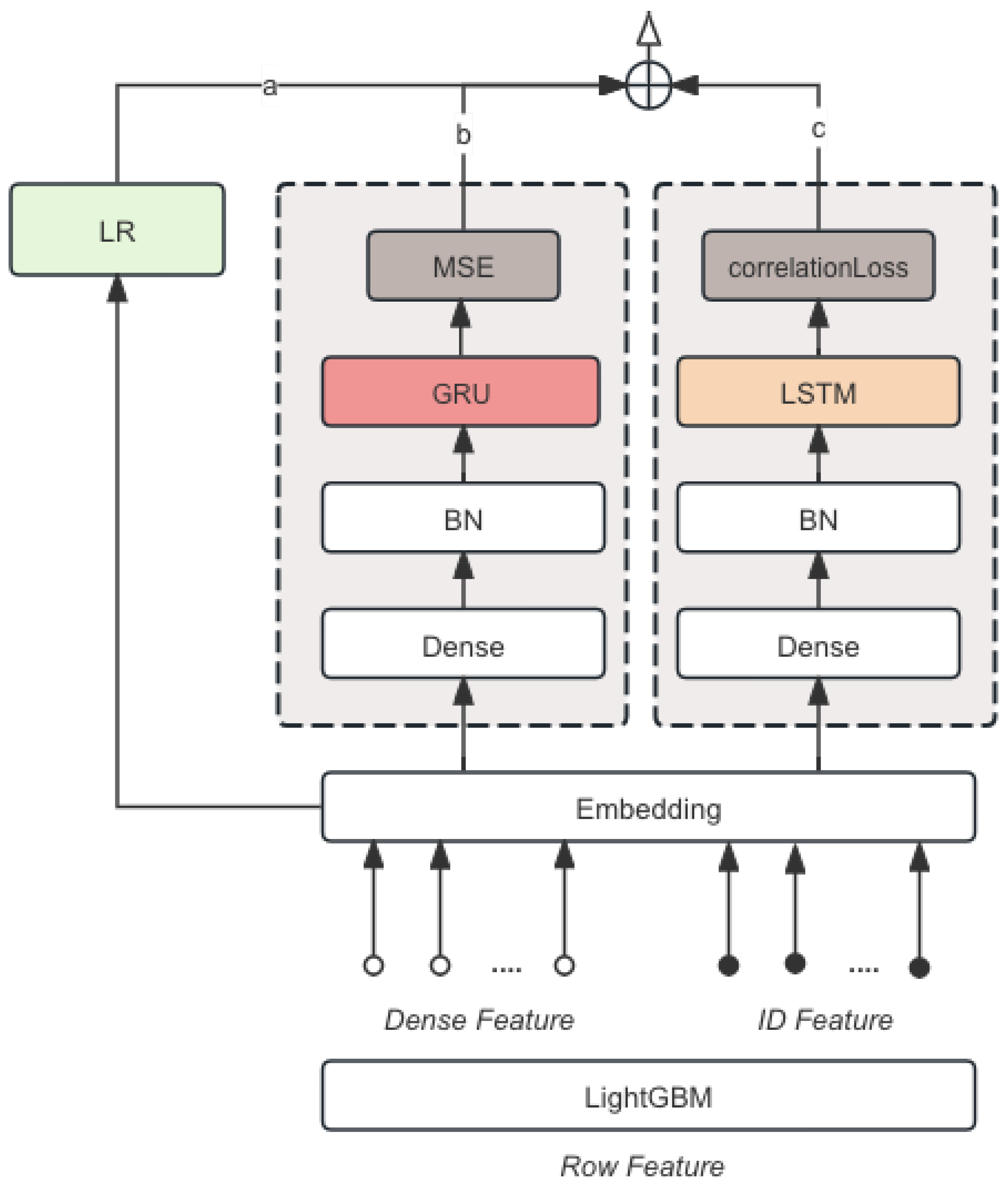

Table 1.
Performance Metrics
| Model | RMSE | Correlation Coefficient |
|---|---|---|
| LightGBM | 0.172 | 0.182 |
| LSTM | 0.214 | 0.234 |
| Keras DNN + RNN | 0.261 | 0.245 |
| Keras DNN + Lightgbm | 0.315 | 0.324 |
| LSTM + GRU + LR + LightGBM | 0.351 | 0.362 |
Disclaimer/Publisher’s Note: The statements, opinions and data contained in all publications are solely those of the individual author(s) and contributor(s) and not of MDPI and/or the editor(s). MDPI and/or the editor(s) disclaim responsibility for any injury to people or property resulting from any ideas, methods, instructions or products referred to in the content. |
© 2024 by the authors. Licensee MDPI, Basel, Switzerland. This article is an open access article distributed under the terms and conditions of the Creative Commons Attribution (CC BY) license (http://creativecommons.org/licenses/by/4.0/).
Copyright: This open access article is published under a Creative Commons CC BY 4.0 license, which permit the free download, distribution, and reuse, provided that the author and preprint are cited in any reuse.