

Submitted:
24 September 2024
Posted:
26 September 2024
You are already at the latest version
Abstract
This study presents a comprehensive investigation on an innovative mechanical system inspired by recent advancements in metamaterials, more specifically the work is focused on Origami-type structures for their intriguing mechanical properties. Originating from the specific fields such as aerospace for their lightweight and foldable characteristics, Origami mechanical devices exhibit unique non-linear stiffness, in particular, when suitably designed, they show Quasi-Zero Stiffness (QZS) characteristics within a specific working range. The QZS property, aligned with the High Static Low Dynamic (HSLD) stiffness concept, suggests promising applications such as a low-frequency mechanical passive vibration isolator. The study explores the vibration isolation characteristics of Origami-type suspensions, with a particular emphasis on their potential application as low-frequency passive vibration isolators. The Kresling Origami Module (KOM) has been selected for its compactness and compatibility with 3D printers. A detailed analysis using 3D CAD, Finite Element Analysis, and experimental testing have been carried out. The investigation includes the analysis of the influence of geometric parameters on the non-linear Force-Displacement curve. Multibody simulations validate the low-frequency isolation properties within the QZS region, and disparities in dynamic properties beyond the QZS range. The study underscores the transformative potential of Origami-type metamaterials in enhancing low-frequency vibration isolation technology. It also highlights challenges related to material properties and loading mass variations, providing valuable insights for future developments in this promising field.
Keywords:
quasi-zero stiffness
; origami-type structure
; non-linear stiffness
; passive vibration isolator
; multibody dynamics
; experimental testing
; metamaterials
1. Introduction
Quasi-Zero-Stiffness mechanisms primarily involve combinations of negative and positive stiffness elements to achieve a stable equilibrium point with very small stiffness. The simplest QZS mechanism proposed in the literature is the planar three-spring vibration isolator [1]. It consists of three springs, with one in the vertical direction connected to the ground and the suspended mass in its unloaded configuration, while the other two springs are in an oblique position. Loading this mechanism with a properly sized load results in spring compression until the equilibrium position is reached. Around this position, the vertical spring behaves as a positive stiffness element, while the two transversal springs, now in the horizontal direction around the equilibrium point, act as negative stiffness elements. One interesting aspect of this solution is that the working position of the mechanism can be tuned using springs with different stiffness characteristics. Kovacic et al. [2] used the same three-spring QZS mechanism, but instead of having all the springs with linear characteristics, the oblique springs had softening nonlinear stiffness characteristics. This configuration resulted in a smaller overall stiffness at larger displacements from the equilibrium position than the system using only linear springs. Various solutions derived from this base arrangement are explored, such as the one presented in Ref. [3], featuring two pairs of oblique springs instead of one. This configuration led to lower dynamic stiffness in a wider region around the equilibrium point and lower force and displacement transmissibility than the original mechanism. Again, on three-spring-based mechanisms, an intriguing solution is presented by Lan et al. [4], this work introduced a three-spring QZS compact mechanism composed of specially designed planar springs with linear stiffness characteristics, deviating from the conventional coil springs. The proposed solution not only exhibited the sought QZS behavior but also offered advantages in terms of design flexibility, as planar springs can be tailored with arbitrarily selected stiffness, and compactness, as they occupy less space than coil springs, optimizing the overall structural design. A slight variation from the three-springs based mechanism involves scissor-like structures arranged symmetrically, see Ref. [5]; this configuration presents an isolator with four n-layer scissor-like structures connected to the four sides of the object to be isolated; moreover, a damper with linear characteristics is added. While this solution increases system complexity due to additional adjustable parameters influencing overall behavior, the heightened complexity could potentially enhance isolation performance across diverse working environments. Another mechanism employing multiple layers of scissor-like structures is introduced by Sun et al. [6], it is designed for vibration isolation in the two directions orthogonal to the vertical axis. Alternatively, achieving a QZS characteristic with a scissor-like structure is demonstrated using only two springs and a series of rigid bars, see Ref. [7]; the vertical spring supports the external load, while the horizontal spring, in conjunction with the symmetric arrangement of the mechanism, induces deformation primarily in the vertical direction; attaining the QZS behavior is possible through careful tuning of the stiffness characteristic and adjusting the length of the bars.
The three-springs mechanism is not the only approach to achieve QZS behavior. Nonlinear isolators can also manifest a negative stiffness characteristic around their working displacement, and to attain QZS behavior, they can be coupled in parallel to a linear spring with a positive stiffness characteristic. This configuration was proposed by Ye et al. [8] utilizing a cam-roller mechanism, comprising a series of cams in the axial direction attached to one end of the main spring-damper system and a roller structure attached to the other end. Similarly, Zuo et al. [9] introduced a cam-roller QZS mechanism, resembling a three-springs mechanism where the mass to be insulate is attached to a cam roller structure, situated above the loading support; they conducted a study on the cam profile and its impact on the isolation performance.
A distinct approach to achieve a negative stiffness characteristic involves the use of the Euler buckled beam. When a perfect slender beam is fixed on one side and axially loaded, after exceeding the critical load, the straight configuration is unstable, as the beam presents a negative stiffness; the buckled beam can be coupled with an elastic spring, to achieve a QZS-like characteristic. Various mechanisms leverage this theory to create nonlinear isolators, as shown e.g., in Ref. [10], which features a planar mechanism with a linear isolator attached to the isolated mass and two buckled beams connected to the mass, in a similar fashion of the three-springs mechanism. A similar system was proposed for shock vibration control by Huang et al. [11]. Effects of transversal springs on slender structures was addressed in Ref. [12] in the framework of the Normal Form theory.
Given that adjustable stiffness is one of the distinctive properties of mechanical metamaterials and metastructures, their application in vibration isolation is noteworthy. Metamaterials and metastructures allow for the programming the mechanical properties through several design parameters. Nowadays they can be easily manufactured using 3D printing technologies, mitigating challenges associated with complex geometry. A mechanical metamaterial having vibration isolation properties was created [13] by Zolfagharian et al. using two distinct unit cells, one stiffer than the other, arranged geometrically to form a cylindrical metamaterial, simulations and experimental tests demonstrated QZS behavior and superior vibration isolation compared to conventional isolators. The mechanical properties of origami-based vibration isolators heavily rely on the crease pattern, which changes with different folding geometries [14]. In general, two methods are considered to design such isolators:
- (1)
- optimization of structural parameters, eliminating the negative stiffness feature caused by oblique creases to achieve QZS characteristics for the entire structure, this is beneficial for high-performance vibration isolation.
- (2)
- Incorporating a parallel spring with positive stiffness into the mechanism to achieve vibration isolation over a broader range, serving as a stiffness corrector.
The present study presents a comprehensive investigation of an innovative mechanical system inspired by recent developments in metamaterials and metastructures, specifically focusing on the vibration isolation properties of Origami-type structures. Origami mechanical equipment, developed in the aerospace sector, where the system might experience complex behavior [15,16] due to characteristics of different components within the system[17,18], for their lightweight and foldable features, represents distinctive non-linear stiffness. The QZS property, aligned with the High Static Low Dynamic stiffness concept, suggests promising applications as a low-frequency mechanical passive vibration isolator. The present study is based on both numerical simulations (Nonlinear Finite Element Method) and experimental testing; the Origami KOM concept chosen for its compactness and compatibility with 3D printers. The investigation delves into geometric parameters’ influence on the Force-Displacement QZS response, resulting in the creation and testing of a KOM prototype. Multibody simulations validate the low-frequency isolation properties within the QZS region, acknowledging challenges associated with material properties and loading mass variations. Overall, this study emphasizes the transformative potential of Origami-type metamaterials/metastructures in advancing low-frequency vibration isolation technology.
2. Vibration Isolation Model
Vibration isolation can be provided using different systems such as: active vibration isolation systems, semi-active vibration isolation systems, and passive vibration isolation systems. The passive vibration isolator is based on a spring and a damping element with linear characteristics, mounted between the vibration source and the object that must be protected from excessive vibrations; this system basically behaves like a single-DOF mass-spring-damper oscillator. Other passive isolators are based on the concept of antiresonance and consist of adding suitable oscillators to the main structure, see e.g., Ref. [19].
One important parameter used in Engineering to evaluate the isolation performances is the transmissibility , it is a dimensionless parameter (at least depending on the frequency of excitation), which is defined as the ratio between the amplitude of the transmitted dynamic force and the corresponding static force or the ratio between the vibration amplitude of the suspended system and the support.
depends on the ratio between the excitation frequency and the natural frequency of the system. In order to have a proper system isolation, should be lower than 1. It can be noticed that , for any value, when the ratio , for higher frequencies, by increasing the , the transmissibility decreases. It means that the isolation is not provided at excitation frequencies less than . Indeed, if a wider isolation region is required, it would be a solution to change the isolation properties.
The Origami considered in the present study is a HSLD stiffness vibration isolator, where the system has a high static stiffness, useful to have a low static displacement, and a low dynamic stiffness, useful for a proper isolation to reduce the natural frequency and to increase the isolation region [20]. The vibration isolator can achieve a QZS around the equilibrium point. This characteristic behavior is due to a highly nonlinear Force-The force displacement curve is shown in Figure 1, the system does not stand the Hook’s law [21], and the stiffness presents a minimum in a wide central interval of displacement and increases for low and high force levels.
The QZS mechanism is typically composed of positive and negative stiffness elements. In this study, an Origami-based metastructure is used to propose the QZS-vibration isolator. The main characteristics of the origami-based metamaterial are foldability, multi-stability, and nonlinear stiffness.
3. The Origami Metastructure
Origami has a complex and repetitive geometry layout, which can achieve interesting mechanical properties. There are different folding geometries which affect the overall shape and behavior of the system, one of which is the Kresling pattern (KOM). The reason for choosing this pattern, KOM, is the size of the geometry and easiness in producing.
Kresling Pattern
The Kresling pattern was initially proposed by Kresling [22] to produce foldable and deployable structures, then it has also been used to propose a new type of origami-based metamaterial. This geometric pattern is based on a series of triangle shaped facets arranged in a cylindrical manner to form a tower-like structure with a hexagonal base, middle and top plane, see Figure 2 and Ref. [23]. The middle plane of the unit cell is the symmetric plane of the mechanism. This symmetrical condition, during the compression of the element, leads to the rotation and translation of the sole middle plane, while the top and base plane will just have a pure translation in the motion direction. The motion of the whole mechanism is like the one of a threaded screw into a nut [24]. The base unit can be stacked in series or in parallel to achieve different vibration isolation performances. This geometric pattern is not under the rigid origami theory, so, when a compressive load is applied, the triangular panels will slightly deform and store the applied work in the form of strain energy. The same strain energy will then be released after the removal of the load and the mechanism will return to its unloaded shape. This mechanism can also have a bistable behavior. In fact, if properly designed, during the motion there could be a second stable configuration.
4. Geometry Definition
The geometry is defined starting from the one proposed in Refs. [25,26]. Five different types of Origami are analyzed: KOM 0, KOM I, KOM II, KOM III, KOMIV. The geometric parameters used in the following investigations are shown in Table 1.
KOM-0: KOM-0 precisely replicates the geometry of the external planar facets in KOM, see Figure 3a. The initial configuration comprises the base and a hexagon inscribed within a circle. The top plate is positioned at a specified distance and angular shift from the base hexagon. Subsequently, two primary triangles are constructed, aided by intersecting construction planes at the middle of structure and aligned with the base and top hexagon planes. A circular pattern of these triangles is generated to finalize the lower structure. The concluding step involves mirroring the existing structure on the top plane, resulting in the completion of the surface model. It is worth mentioning that KOM-0 has flexures instead of joints with rotational springs.
KOM-I: The focus of KOM-0 is on effectively modeling the creases, with the goal of imparting a rotational spring-like behavior. This behavior can be achieved by ensuring that the thickness of the crease is less than that of the corresponding facet. In the case of KOM-I, a central core is added to each base triangular facet with a specific thickness. The creases are then modeled around this core, having a thickness equal to half of the core thickness in the initial analysis. The final stages involve assigning suitable thickness to the base, middle, and top planes, Figure 3b.
KOM-II: The idea of KOM-II model is rooted in manufacturing considerations regarding KOM-I; due to numerous geometry variations in different directions achieving precise replication during manufacturing poses a challenge. To address this issue, a straightforward solution is to create walls with uniform thickness, see Figure 3c, and to better reproduce a rolling-joint behavior on the edges, the central parts of the faces are thickened extruding a triangular feature. All other procedural steps and geometric features in KOM-II remain consistent with the previous models, Figure 3c.
KOM-III: The KOM-III model closely mirrors the KOM-II model, with the key distinction lying in the introduction of a fillet at the connection between the extruded core triangles and the side triangles. Notably, this fillet replaces the sharp edge present in the KOM-II model. The fillet radius matches the dimension of the core triangle thickness, a deliberate choice aimed at minimizing the number of geometric parameters. This strategic decision is made under the consideration that the fillet’s impact on the overall system behavior is minimal, Figure 3d.
KOM-IV: the last Origami structure is KOM-IV, this variation has been designed to explore different scenarios and check the effect of a truss-like structure, where instead of having a solid triangular core there was a triangular hole in the middle of the triangular faces, Figure 3e.
KOM-II and KOM-III are simplified models in order to address manufacturing concerns. Further variants of KOM are KOM-Ia, KOM-IIa, KOM-IIIa and KOM-IVa, which are basically the same models presented previously; however, the intersecting construction plane at the middle of structure and aligned with the base and top planes is removed, see Figure 3-version a.
5. Numerical Analysis on the Influence of Design Parameters on the Origami Stiffness
Due to the complexity and nonlinearity of the Origami structure, it is essential to evaluate the behavior of the system under different load conditions and design parameters. The numerical analysis is carried out using the FEM-based software NASTRAN. The aim is to correlate FEM simulations with experimental tests, in order to set and validate the numerical model. The material is Polylactic acid, a common thermoplastic used in 3D filament printing, see Table 2.
The FEM analysis relies on a static nonlinear simulation, even though the primary concerns pertain to the system’s dynamic behavior; indeed, the goal is to determine the elastic characteristics of the Origami, i.e., the force-displacement curve. To gauge the restoring force exerted by the mechanism during the compression stroke, a Rigid Body Element is applied at the midpoint of the top face, connecting to all associated nodes. the base plane and the midpoint of the top face are fixed to ensure a statically determined structure. Eventually, the compressive load is applied at the RBE node.
5.1. Element Selection for FEA
The initial step is to select the appropriate element to represent the Origami. Given that the mechanism relies on planar oblique facets and horizontal plates, both solid elements and shell elements are viable options. On the KOM-0 and KOM-I models, we analyzed which of the two elements (solid or shell) would best suit our purposes, Figure 4 shows the FEM mesh for the two types of elements. In order to assure sufficient accuracy, a parabolic formulation was applied to both finite elements. The simulation parameters are shown in Table 3.
The overall behavior of the system aligns with expectations, featuring a swift force increase leading to a maximum, followed by a gradual force decrease. Analyzing Figure 5 reveals almost identical force responses for both quadrilateral shell elements and tetrahedral solid elements, indicating their interchangeable use without introducing modeling errors. The primary distinction arises in simulation time, with quadrilateral shell elements significantly reducing the time required by over half compared to tetrahedral solid elements. However, it is noted that shell elements may not accurately replicate crease geometry due to their formulation, designed for structures with a substantially smaller thickness dimension. Consequently, the preference going forward is to primarily employ solid element formulation, reserving the use of shell elements for instances where simulation time becomes excessive.
5.2. Stiffness Analysis
In this section a comparison between the eight models (KOM I-IV and Ia, IIa, IIa, Iva) is carried out, a compressive load is applied, with the aim of understanding their behavior under large displacement. Figure 6 presents the comparison between different models. KOM v2, v3 and v4 have a stiffer response with respect to KOM v1, while KOM v1a and KOMv4a are less stiff than KOM0, similar behaviour is found for KOM v2a and v3a.
5.3. Strain Analysis
In this section, the behavior of the Origami’s is evaluated in order to understand if they behave like a mechanism or like a (meta)-structure. This study serves the purpose of determining whether the modeled creases work well as rotational springs, while also examining whether the strain on the planar facets is negligible compared to that of the creases.
For this study, the KOM-I model is considered, loaded with the same compression stroke as in Table 4. This choice is made with the intention of examining the strain distribution around the presumed working stroke. The simulation parameters for this analysis are defined in Table 4.
As shown in Figure 7, the significant difference in strain amplitude between creases and planar facets confirms that the Origami behaves mostly like a mechanism. The motion of the KOM primarily relies on the rotation and deformation of creases, with a lesser contribution from the bending of lateral facets.
5.4. Analyzing the Effects of the Middle Plane Shift Angle
Understanding how design variables influence the attitude of the system is crucial for suitably setting the Origami as a nonlinear suspension. In this section, we analyze the KOM-I model with varying middle plane angular shifts. The base model initially features a 30° angular shift between the base plane and the middle plane, see Figure 8.
To avoid introducing modeling errors, the lower and upper limits of this angle were determined from the 3D model, with the lower limit at approximately 16° and the upper limit at around 55°. This sensitivity analysis uses a shell element model subjected to a 10 mm compressive stroke, with an angular variation of 10° between planes for each simulation. To reduce simulation time, the shell element is used for this analysis. The simulation parameters are detailed in Table 5.
In Figure 9 the force displacement curves for different angles are shown, it is evident that an increment of the angular shift between the base and middle planes results in a substantial decrease in the force response. Specifically, the maximum force for the case with the shift angle equals to 50° is something more than 50% of the maximum observed for the case with the angle equals to 20°. Additionally, achieving the QZS behavior in the system becomes more challenging when there is a smaller initial angular shift between the two planes. In Figure 9, the stiffness curve for the case with the shift angle equals to 50° consistently remains above the horizontal line representing zero stiffness, albeit in close proximity. For the case with the angle equals to 20°, the simulation ceases at approximately half of the overall stroke values. Although the simulation stops, it is noteworthy that excessively reducing the shift angle can cause a significant reduction in force, potentially leading to undesired system instability.
5.5. Analyzing the Effects of the Distance between Middle Plane and Base Plane
In this section, the analysis involves varying the distance between the base and the middle plane. This variation directly impacts the overall height of the Origami, potentially influencing the compressive strokes due to the compressive load. In order to maintain consistency across these studies, we opt to use a constant compression stroke for all simulations, facilitating a coherent comparison of results across different design parameters.
The initial step involves determining the lower and upper limits for the height of the model, represented by the distance between the base and middle plane. In this case, the lower height limit is set to 6 mm. As there is no proper upper limit due to the fact that the system potentially behaving like a vertical tower-like structure, we decide to commence the analysis from a 10 mm distance between the two planes, resulting in an overall height of 23 mm, considering the base, middle, and top planes.
This starting value is increased by a 4 mm shift until reaching a 26 mm distance between the two planes, corresponding to an overall height of 55 mm. The simulation parameters are consistent and detailed in Table 5.
In Figure 11a, the force-displacement curve is represented, it is evident that an increase in the height of the middle plane results in a more pronounced force reduction after reaching its maximum. This trend is further clarified in Figure 11b, showing the stiffness of the Origami, where the curve for the 26 mm height stays below the horizontal line representing zero/negative stiffness for an extended distance. This indicates that, in this particular case, the system fails to attain the QZS condition. Additionally, consistently with the earlier analysis, the significant force reduction observed here can lead to system instability and that is not welcome for engineering applications.
5.6. Analyzing the Effects of Different Base Length
In this section an analysis of the design parameters is carried out, it focuses on varying base lengths, see Figure 12, while maintaining a constant overall height. For this analysis, there are no strict upper or lower limits for the base length, as its variations solely impact on the overall dimensions of the Origami. Since the proposed system is intended for use as a mechanical vibration isolator, the dimensions of the mechanisms may pose challenges during production and mounting, excessively small should be avoided.
To address this concern, the lower base length limit for the study is set at 6 mm, incrementally increasing by a 4 mm shift until reaching a maximum base length of 26 mm. The simulation parameters align with those detailed in Table 5.
Figure 13a shows the force-displacement curves, it is evident that an increment in base length facilitates a more attainable realization of QZS behavior, i.e., negative stiffness is less likely to appear for larger base length. Notably, this effect is particularly pronounced at extended compression stroke values, despite the uniformity in overall system height across all models under analysis. The scrutiny of Figure 13b (stiffness vs. displacement) reveals that, for base lengths of 18 mm, 22 mm, and 26 mm, the stiffness converges closely to the horizontal line denoting zero stiffness, particularly at higher compression stroke values.
5.7. Analyzing the Effects of Different Planar Facets Thickness
The final analysis of design parameters focuses on varying planar facets thickness. It was anticipated that reducing the thickness of planar facets results in a corresponding reduction in force, indicative of a lower system stiffness. The lower limit for this analysis is set at 0.2 mm, dictated by manufacturing constraints that cannot ensure planar facet thicknesses below this threshold. The upper limit is established at 0.6 mm. The remaining design parameters of the KOM-I Origami are consistent with the basic model KOM-0. An increment of thickness of 0.1 mm will be applied for the analysis, maintaining uniformity with simulation parameters detailed in Table 5. Figure 14 shows the force-displacement curves and the stiffness vs. displacement, it demonstrates a decrease in system force with a reduction in planar facets thickness.
5.8. Conclusions on the Numerical Analysis of Design Parameters
The findings of this analysis underscore the substantial impact that variations in specific design parameters can have on the Origami’s force response. For instance, achieving QZS behavior may necessitate adjustments to both the base length and the angular shift between the base and middle planes. It is important to note that all the considered variations thus far have been undertaken without knowledge of the mass requiring isolation by the mechanism. A more targeted approach could involve initiating the design process with a known isolated mass and subsequently adjusting the design parameters to achieve QZS behavior at the required displacement.
6. Dynamic Simulations: The Multibody Dynamics Model
In this section, the dynamic properties of a KOM system are numerically investigated through a nonlinear dynamical model. The software MSC ADAMS is used here, it is one of the most reliable Multibody Dynamics software used in engineering. The focus of the investigation is the KOM’s dynamic properties, which are essential for understanding the HSLD and QZS characteristics.
This model is based on a spring-mass system, omitting damping effects on the spring element. Figure 15 shows the graphical representation of the Multibody model, the red box represents the base undergoing to a seismic-like motion. The green box represents the mass, conceptualized as an ideal cubic-shaped mass. A translational joint connects its center of mass (CM) to the base, i.e., the mass is constrained to move in the vertical direction relative to the base only. The coil spring serves as the translational spring, linking the CM of the mass to the base CM. In the basic formulation of a traditional elastic suspension, the spring is linear, i.e., the force is proportional to the displacement through a constant stiffness. In the case of Origami KOM’s, having the focus on QZS properties, a suitable force-displacement law is set in the Multibody software, which calculates the stiffness based on the given law.
Therefore, the input for the Multibody model is the Force-Displacement curve of the KOM mechanism obtained through nonlinear FEM simulations or from experimentation. This curve will serve to define the non-linear behavior of the spring during the compression stroke. Furthermore, the QZS range and the input data for mass is derived from this curve, ensuring the equilibrium point of the system lies within the range where the force-displacement curve is almost flat (minimal tangent stiffness). The Multibody simulations are carried out for the KOM-II, KOM-IIb Origami’s. The KOM-IIb has the HSLD characteristic and a near QZS characteristic, which avoids the negative tangent stiffness behavior that leads to system instabilities, i.e., negative slope of the force-displacement curve. The model parameters are shown in Table 6.
In Figure 16a, the comprehensive Force-Displacement plot illustrates both tractive and compressive strokes applied to the KOM-IIb from nonlinear FEM model, note that now the FEM analysis is extended to negative (tractive) displacements, as they are likely to take place during a real dynamic scenario. Positive displacement and force correspond to the compressive phase, which is of particular interest for this work, while negative displacement and force values pertain to the tractive phase, which can be experienced in particularly violent resonances. Figure 16b further delineates the QZS region and two additional characteristic regions within the compression stroke. This subdivision within the working range of the mechanism is valuable for highlighting the distinctions observed at different working points, see Figure 17. Of primary interest is the QZS region, spanning from +4 to +8 mm, where the Origami’s stiffness, although not exactly zero, assumes a minimal value compared to the stiffness in the other two working regions.
The operational point of the KOM-IIb is positioned in the middle of the QZS zone, specifically at a compression stroke of 6 mm, see Figure 17: case-II; for such deflection. the reaction force of the Origami is 1518.32 N, corresponding to the weight of a mass of 154.77 kg. Such mass (see the red box in Figure 15) is used in the Multibody model together with the gravity acceleration in the direction of the mass motion. Once these parameters are set, the model accurately reflects the expected operation of a KOM system. Now the mechanism operates around its equilibrium point as a QZS, due to the suitable value of the mass/weight. Different working conditions will be systematically analyzed by adopting various spring preloads to elucidate the system’s dynamic response.
The seismic like motion imposed to the base CM is a sine-sweep ( where is the lower frequency, is the upper frequency and is the sweep duration) with a constant amplitude of mm, such kind of signal, which dynamically varies the frequency over time from an initial to an ending frequency , is commonly used in simulation and experimentation for investigating non-linear dynamic scenarios: resonance frequencies and magnification factors. This kind of excitation is suitable for a basic evaluation of the isolator performances, even though for deeper analyses of the nonlinear behavior, the stepped sine approach can give more insight on the nonlinear dynamic scenario, see e.g., Ref. [28].
The next step is to carry out different simulations aimed at understanding how Origami based suspensions respond to sinusoidal seismic excitations; no damping is included in the system. The results are analyzed in the frequency domain by calculating the Frequency Response Functions for both magnitude and phase, the MSC ADAMS VIBRATION PLUGIN is used for such a purpose. The workflow of this plugin begins with defining the equilibrium point of the system, followed by model linearization around that point, and ultimately conducting vibration analysis on the linearized model. The simulation is done for three different cases from different regions: case-I, case-II, and case-III; besides, all simulation parameters are defined as shown in Table 7.
Case-I (PRE QZS region): In this case, the equilibrium point is set to be in the PRE QZS region, and to reach this specific working region, a spring preload is applied. It is assumed that the new equilibrium point will be at a compression stroke value of 2 mm. The stiffness is determined from FEM data, and to achieve the equilibrium point, a spring preload is used since the mass and the static load should give equilibrium in the QZS zone, but we want that the Origami operates in a different zone. To attain the PRE QZS working point, a spring preload is applied in the vertical direction (positive y direction), effectively reducing the compressive stroke of the spring element. The natural frequency observed in this configuration is now 6.3152 Hz.
Case-II (QZS region): the equilibrium point is in the Quasi-Zero Stiffness region, where the system is expected to operate in an optimal condition. The stiffness is derived from FEM data, and in this case, no spring preload is necessary since the weight associated to the mass gives the equilibrium in this region. It is expected that the new equilibrium point is at a compression stroke value of 6 mm, resulting in a natural frequency of 0.8640 Hz.
Case-III (POST QZS region): In this case, the equilibrium point is situated in the POST Quasi-Zero Stiffness region, requiring the application of a spring preload in the opposite direction compared to Case-I. It is assumed that the new equilibrium point will be at a compression stroke value of 9 mm. The stiffness, derived from FEM data, necessitates the application of a spring preload to achieve the predefined equilibrium point since the mass and the static load should give equilibrium in the QZS zone, but here there is interest in the POST-QZS. To attain the POST QZS working point, a spring preload is applied in the vertical direction (negative y direction), effectively increasing the compressive stroke of the spring element. The natural frequency observed in this configuration is 1.6259 Hz.
The performances of the isolator are here evaluated through the analysis of transmissibility, even though more sophisticated signal processing techniques are available in literature, see e.g., Ref. [29], for the purpose of the present work, the transmissibility analysis is considered sufficient for evaluating the basic performances.
Figure 18 shows that the behavior of the system depends on the working position. The x-axis of the graphs is normalized based on the natural frequency of the system in the QZS working position. For Case-II, at the QZS point, the KOM exhibits the lowest resonance frequency compared to those of the POST-QZS (case-III) and PRE-QZS (case-I) points. This finding is crucial because if the system operates in the QZS position, it initiates the suppression of excitation from the base at a lower frequency in contrast to the other working positions. These three simulations, Case-I, Case-II, and Case-III have been carried out assuming small oscillations around the equilibrium points, in this way the linearity hypothesis is still valid. However, it must be point out that the nonlinear character of the system is not lost, as the equilibrium position and the consequent linearization, vary depending on the static load; this is a direct consequence of the nonlinearity.
7. Experiments on Origami Suspensions
The test case considered for the experiments is based on KOM-III, indeed, the QZS region for this model presents reasonable force values. Eight distinct cases, all based on KOM-III, are considered; each case is described by the geometric parameters shown in Table 8. In order to enhance our understanding of the Force-Displacement characteristics of the proposed geometries, an additional analysis involves applying a tractive load with a constant stroke of 10 mm, see Table 8.
Before conducting the experimental test, some initial steps are required to suitably set all parameters. First of all, a FEA is carried out to evaluate the main differences between all geometries; Figure 19 represents numerical results for all cases. The results reveal similarities in the behavior of the system in terms of force-displacement and stiffness diagrams. Therefore, KOM-III.3 is considered as the main model to produce and carry out the experimental analysis, this particular case was selected due to the absence of negative stiffness, and the zero-stiffness zone is activated with an adequate but not overly excessive displacement. This is done to prevent any abrupt jump effects in the system.
The second step is to select the material for the 3D printing, which uses a fused filament fabrication process and a thermoplastic material filament. Two types of materials are considered (PLA and TPU), which are commonly used for 3D printed components. The principal nominal mechanical properties of these materials are listed in Table 16; it is worthwhile to point out that these values can significantly vary during the printing process due to several factors: moisture, room temperature, extrusion temperature, material contamination. Before conducting the experimental text, a numerical simulation is conducted for each material, utilizing the KOM-III.3 Origami under a compression of 38 mm. This simulation aims to determine the most suitable material for the prototype and subsequent tests.
The results represented in Figure 20 show that the force levels that lead to the QZS region greatly vary for different materials and we are interested to the lowest, because it is in the force range of our load cell experimental setup ; this is achieved with the TPU filament, see Figure 20b. Once all parameters has been set, we proceed with the next step that involves the 3D printing of the KOM-III.3 prototype, see Figure 21.
7.1. Experimental Static Tests: Measurement of the Nonlinear Stiffness
The main purpose of these compressive tests is to carefully study how the KOM prototype behaves in terms of force-displacement dependency. The goal is to check if the QZS behavior identified in the numerical model is confirmed experimentally. This investigation is crucial for ensuring the reliability and practicality of the numerical model of the KOM Origami in real-world applications.
The test setup, shown in Figure 22, comprises a metal plate to which a metallic cube is connected on one side (right side in Figure 22) and a screw attached to a thin metallic circular plate on the other side (left side in Figure 22). Positioned between the screw and the circular plate there is a load cell, essential for measuring the force exerted by the KOM during the compressive stroke. The final component of the test setup is a mechanical comparator that determines the displacement of the circular plate during compression. The KOM prototype is situated between the cube and the plate, supported by a circular support (white color in figure). The entire assembly is securely clamped to a sturdy metallic plate to prevent any minute base movements that could compromise the accuracy of the measurements.
This static test involves a 40 mm compression stroke, with 1 mm increments, the force is measured by a load cell with an acquisition device. Six compressive tests have been conducted using this setup. Among them, three tests will position the KOM model with the upper part on the left side, while the remaining tests position the upper part on the right side. Additionally, the prototype is rolled around its axis between each compression. Varying the model’s positions during the tests aims to mitigate the impact of manufacturing imperfections and enhance the influence of the system’s geometry on the resulting Force-Displacement characteristics.
Figure 23 illustrates the experimental results, where a subtle QZS behavior emerges within the compressive stroke range of 10 mm to 20 mm. In Figure 23b, the results have been averaged, and the resulting curve has been interpolated using an eighth-order polynomial. The Force-Displacement averaged data has been utilized to define the Stiffness-Displacement characteristic in Figure 23b interpolated with a seventh-order polynomial. These interpolations distinctly reveal the presence of the QZS property in the prototype.
7.2. Numerical-Experimental Correlation
Once the experimental measurements and processing have been completed and the Force-Displacement characteristics are estimated, the final step of this work involves refining the FEM and Multibody models used in the preceding sections to fit the real KOM’s behavior. Initially, the FEM model is set to obtain the Force-Displacement characteristic of the virtual model corresponding to the experiments. This virtual characteristic is then compared to the experimental one to highlight any discrepancies. Subsequently, both characteristics are employed, to refine the Multibody model and define its dynamic properties. This point is required to repeat that KOM-III.3 is considered for carrying out the simulations.
7.3. FEM Correlation
The first step of the correlation analysis is to establish a FEM model that accurately replicates the results obtained from the experimental tests. Throughout the 3D printing process, the mechanical properties of the materials may exhibit significant variations from their nominal values, indeed, they are influenced by several environmental factors. Another distinction between the modeled and 3D printed KOM lies in the manufacturing process. The KOM model is directly derived from the 3D CAD model. It incorporates sections between two external walls that are uniformly filled with material distributed in an ideal manner. However, the 3D printed model may exhibit slight differences due to the manufacturing process. Factors such as infill parameters, density, geometric pattern, orientation, and wall thickness can be defined prior to the 3D printing process. Each of these factors significantly impacts the mechanical response of the 3D printed model. [30]. The parameters, modified to fit the experimental test, are the material properties (isotropic): Young’s Modulus (E) and Poisson coefficient (). The first study is conducted by varying the Young’s Modulus and considering TPU material with constant Poisson coefficient, i.e., the TPU nominal one, this range spans from 14 MPa to 7 MPa [31].
The results of the simulation are presented in Figure 24, which displays the Force-Displacement characteristics of the models at different Young’s Moduli (E). In Figure 24, the error for each FEA is defined by considering the experimental results as the reference data for two different regions: region 1: and region 2: . Among the simulations, and exhibit the closest fit to the experimental results (blue and red solid line in Figure 24 respectively), considering the overall error. Although the simulation carried out using has a slightly lower overall error, the model chosen for Multibody correlation is the one obtained using . This decision is based on the lower error observed in the compression strokes ranging from 0 to 20 mm (Region 2), a critical zone where the QZS behavior is of particular interest.
In the next step, the Poisson coefficient value is identified to enhance the correlation between experimental and simulation results. Different simulations are carried out by varying the Poisson coefficient around its nominal value, while keeping the Young modulus constant. It was observed that the influence of the Poisson coefficient on the Force-Displacement characteristic is minimal and primarily centered on the last phase of the compression stroke. Consequently, the model to be used in the next section will feature the nominal value for the Poisson coefficient.
The comparison between the Force-Displacement and Stiffness-Displacement characteristics is depicted in Figure 25. The main source of error is concentrated on the final part of the compression stroke, where a significant portion of compression and sliding between adjacent walls occurs.
A significant disparity is observed in the Force-Displacement and Stiffness-Displacement responses between experimental data and the simulated model for larger displacements. This variance was anticipated, as the model does not account for specific simulation factors such as internal contacts and sliding or manufacturing aspects like the internal infill pattern, both of which can impact the system’s response. To quantify these differences in dynamic properties, Multibody simulations were conducted using the Force-Displacement curves from the correlated model and the experimental test. As expected, discrepancies up to the QZS region were below 10%, but the error increased beyond the QZS region. The study affirms the potential of the technology, particularly in low-frequency vibration isolation, with versatile applications across various industries. However, the complexity arises from the interaction of the working principle across different engineering fields, and material properties and loading mass variations notably influence the system’s response.
7.4. Multibody Correlation on FRF
The final step is to analyze the dynamic behavior of the system, using the experimental and FEM stiffness. The single-DOF multibody model, implemented in MSC ADAMS, has been used for this purpose.
In Figure 25, the properties used to define the spring stiffness of the equivalent single-DOF for both models are presented; for the dynamic simulations three different working positions are evaluated, see Table 9. In the QZS position of both models, the corresponding loading mass value is defined, followed by the application of the same base excitation used in the prior Multibody simulations. In these simulations, the base excitation frequency ranges from 0 to 15 Hz, and only the undamped configuration is analyzed for this model.
Figure 26 and Table 10 show that the FEM model aligns well with the experimental data in the PRE-QZS and QZS regions (blue box and red box in Figure 26), exhibiting an error for the natural frequencies in those working zones of less than 10%. The model spring characteristics, mimicking the KOM system, closely resemble the curve presented in Figure 25, particularly in the first two working zones. Conversely, a notable error is expected in the POST-QZS working zone, highlighting the substantial difference between the experimental stiffness and the FEM stiffness.
8. Conclusions
This study investigates a novel mechanical system inspired by metamaterials, specifically an Origami-type (meta)structures, renowned for their unique mechanical properties. Focusing on the vibration isolation characteristics, the Origami model, when appropriately designed, exhibits a Quasi-Zero Stiffness property within its working range, offering promising applications as a low-frequency mechanical passive vibration isolator.
Among various Origami-based metamaterials, each featuring distinct geometric patterns, the KOM was selected for its compactness, folding motion, and compatibility with common 3D printers. By modeling the Origami through a 3D CAD software and deriving different FEM models, we investigated the influence of key geometric parameters on the non-linear Force-Displacement QZS characteristics. The objective was to identify the most influential parameter in shaping the Force-Displacement dependency and leverage this knowledge to create a KOM prototype for testing. Subsequently, a Multibody software was used to explore the dynamic properties of the system, confirming low-frequency isolation properties with low compression strokes in the QZS region. This is achievable with proper isolator design and the correct loading mass. Following a numerical study of the system without constraints on loading mass or KOM dimensions, the goal shifted to creating a prototype using a 3D printer. The prototype was statically tested to validate the properties predicted by FEM simulations. Once the Origami prototype was produced, experimental tests were conducted and the Force-Displacement characteristic were obtained, confirming the QZS properties. The final step involved proposing a correlation between the data obtained from experimental tests and the virtual model of the prototype. The initial correlation analysis was conducted using FEM software, resulting in a Force-Displacement curve of the model that aligns with the experimental data until the end of the QZS region.
Funding
STARTER KIT FAR Dipartimentale 2022 nr 3482 for the project “Identification, modelling and analysis of nonlinear EMG signals of pathological tremor”.
Conflicts of Interest
The Authors declare that there is no conflict of interest.
Abbreviations
| CAD | Computer Aided Design |
| CM | Center of Mass |
| DOF | Degrees of Freedom |
| FEA | Finite Element Analysis |
| FEM | Finite Element Method |
| FRF | Frequency Response Function |
| HSLD | High-Static-Low-Dynamics |
| KOM | Kresling Origami Module |
| PLA | Polylactic acid |
| QZS | Quasi-Zero-Stiffness |
| RBE | Rigid Body Element |
| TPU | Thermoplastic Polyurethane |
References
- A. Carrella, M. J. Brennan, and T. P. Waters, “Static analysis of a passive vibration isolator with quasi-zero-stiffness characteristic,” J Sound Vib, vol. 301, no. 3–5, pp. 678–689, Apr. 2007. [CrossRef]
- I. Kovacic, M. J. Brennan, and T. P. Waters, “A study of a nonlinear vibration isolator with a quasi-zero stiffness characteristic,” J Sound Vib, vol. 315, no. 3, pp. 700–711, Aug. 2008. [CrossRef]
- F. Zhao, J. C. Ji, K. Ye, and Q. Luo, “Increase of quasi-zero stiffness region using two pairs of oblique springs,” Mech Syst Signal Process, vol. 144, p. 106975, Oct. 2020. [CrossRef]
- C. C. Lan, S. A. Yang, and Y. S. Wu, “Design and experiment of a compact quasi-zero-stiffness isolator capable of a wide range of loads,” J Sound Vib, vol. 333, no. 20, pp. 4843–4858, Sep. 2014. [CrossRef]
- X. Sun and X. Jing, “Multi-direction vibration isolation with quasi-zero stiffness by employing geometrical nonlinearity,” Mech Syst Signal Process, vol. 62–63, pp. 149–163, Oct. 2015. [CrossRef]
- X. Sun and X. Jing, “A nonlinear vibration isolator achieving high-static-low-dynamic stiffness and tunable anti-resonance frequency band,” Mech Syst Signal Process, vol. 80, pp. 166–188, Dec. 2016. [CrossRef]
- G. Gatti, A. D. Shaw, P. J. P. Gonçalves, and M. J. Brennan, “On the detailed design of a quasi-zero stiffness device to assist in the realisation of a translational Lanchester damper,” Mech Syst Signal Process, vol. 164, p. 108258, Feb. 2022. [CrossRef]
- K. Ye, J. C. Ji, and T. Brown, “Design of a quasi-zero stiffness isolation system for supporting different loads,” J Sound Vib, vol. 471, p. 115198, Apr. 2020. [CrossRef]
- S. Zuo, D. Wang, Y. Zhang, and Q. Luo, “Design and testing of a parabolic cam-roller quasi-zero-stiffness vibration isolator,” Int J Mech Sci, vol. 220, p. 107146, Apr. 2022. [CrossRef]
- X. Huang, X. Liu, J. Sun, Z. Zhang, and H. Hua, “Vibration isolation characteristics of a nonlinear isolator using Euler buckled beam as negative stiffness corrector: A theoretical and experimental study,” J Sound Vib, vol. 333, no. 4, pp. 1132–1148, Feb. 2014. [CrossRef]
- X. Huang, Y. Chen, H. Hua, X. Liu, and Z. Zhang, “Shock isolation performance of a nonlinear isolator using Euler buckled beam as negative stiffness corrector: Theoretical and experimental study,” J Sound Vib, vol. 345, pp. 178–196, Jun. 2015. [CrossRef]
- F. Pellicano and F. Mastroddi, “Nonlinear Dynamics of a Beam on Elastic Foundation,” Nonlinear Dyn, vol. 14, no. 4, pp. 335–355, 1997. [CrossRef]
- A. Zolfagharian, M. Bodaghi, R. Hamzehei, L. Parr, M. Fard, and B. F. Rolfe, “3D-Printed Programmable Mechanical Metamaterials for Vibration Isolation and Buckling Control,” Sustainability 2022, Vol. 14, Page 6831, vol. 14, no. 11, p. 6831, Jun. 2022. [CrossRef]
- J. C. Ji, Q. Luo, and K. Ye, “Vibration control based metamaterials and origami structures: A state-of-the-art review,” Mech Syst Signal Process, vol. 161, p. 107945, Dec. 2021. [CrossRef]
- F. Pellicano, A. Zippo, G. Iarriccio, and M. Barbieri, “Experimental Study on Nonlinear Random Excitation,” Lecture Notes in Mechanical Engineering, pp. 637–648, 2020. [CrossRef]
- G. Iarriccio, A. Zippo, F. Pellicano, and M. Barbieri, “Resonances and nonlinear vibrations of circular cylindrical shells, effects of thermal gradients,” Proc Inst Mech Eng C J Mech Eng Sci, vol. 235, no. 20, pp. 4818–4832, Oct. 2021. [CrossRef]
- M. Molaie, F. S. Samani, A. Zippo, and F. Pellicano, “Spiral Bevel Gears: nonlinear dynamic model based on accurate static stiffness evaluation,” J Sound Vib, vol. 544, p. 117395, Feb. 2023. [CrossRef]
- G. Iarriccio, A. Zippo, and F. Pellicano, “Asymmetric vibrations and chaos in spherical caps under uniform time-varying pressure fields,” Nonlinear Dyn, vol. 107, no. 1, pp. 313–329, Jan. 2022. [CrossRef]
- F. S. Samani, F. Pellicano, and A. Masoumi, “Performances of dynamic vibration absorbers for beams subjected to moving loads,” Nonlinear Dyn, vol. 73, no. 1–2, pp. 1065–1079, Mar. 2013. [CrossRef]
- X. Huang, Y. Chen, H. Hua, X. Liu, and Z. Zhang, “Shock isolation performance of a nonlinear isolator using Euler buckled beam as negative stiffness corrector: Theoretical and experimental study,” J Sound Vib, vol. 345, pp. 178–196, Jun. 2015. [CrossRef]
- S. Liu, G. Peng, Z. Li, W. Li, K. Jin, and H. Lin, “Design and experimental study of an origami-inspired constant-force mechanism,” Mech Mach Theory, vol. 179, p. 105117, Jan. 2023. [CrossRef]
- B. Kresling, “Origami-structures in nature: lessons in designing ‘smart’ materials,” MRS Online Proceedings Library (OPL), vol. 1420, pp. mrsf11-1420-oo02-01, 2012. [CrossRef]
- Q. Zhang, J. Cai, M. Li, and J. Feng, “Bistable behaviour of a deployable cylinder with Kresling pattern,” in 7th International Meeting on Origami in Science, Mathematics and Education (7OSME), Oxford University, United Kingdom, 2018. [Online]. Available: https://www.researchgate.net/publication/335925217_Bistable_behaviour_of_a_deployable_cylinder_with_Kresling_pattern.
- S. Khazaaleh, R. Masana, and M. F. Daqaq, “Combining advanced 3D printing technologies with origami principles: A new paradigm for the design of functional, durable, and scalable springs,” Compos B Eng, vol. 236, p. 109811, May 2022. [CrossRef]
- H. Han, V. Sorokin, L. Tang, and D. Cao, “Lightweight origami isolators with deployable mechanism and quasi-zero-stiffness property,” Aerosp Sci Technol, vol. 121, p. 107319, Feb. 2022. [CrossRef]
- S. M. Alipour and J. Arghavani, “On the starting point in designing Kresling origami,” Aerosp Sci Technol, vol. 138, p. 108301, Jul. 2023. [CrossRef]
- S. Farah, D. G. Anderson, and R. Langer, “Physical and mechanical properties of PLA, and their functions in widespread applications — A comprehensive review,” Adv Drug Deliv Rev, vol. 107, pp. 367–392, Dec. 2016. [CrossRef]
- F. Pellicano, M. Barbieri, A. Zippo, and M. Strozzi, “Experiments on shells under base excitation,” J Sound Vib, vol. 369, pp. 209–227, May 2016. [CrossRef]
- L. Gelman, N. Harish Chandra, R. Kurosz, F. Pellicano, M. Barbieri, and A. Zippo, “Novel spectral kurtosis technology for adaptive vibration condition monitoring of multi-stage gearboxes,” Insight: Non-Destructive Testing and Condition Monitoring, vol. 58, no. 8, pp. 409–416, Aug. 2016. [CrossRef]
- M. Qamar Tanveer, G. Mishra, S. Mishra, and R. Sharma, “Effect of infill pattern and infill density on mechanical behaviour of FDM 3D printed Parts- a current review,” Mater Today Proc, vol. 62, pp. 100–108, Jan. 2022. [CrossRef]
- “Home | Covestro AG.” Accessed: Dec. 15, 2023. [Online]. Available: https://solutions.covestro.com/en.
- “Online Materials Information Resource - MatWeb.” Accessed: Dec. 15, 2023. [Online]. Available: https://www.matweb.com/.
Figure 1.
QZS Force-Displacement behaviour.
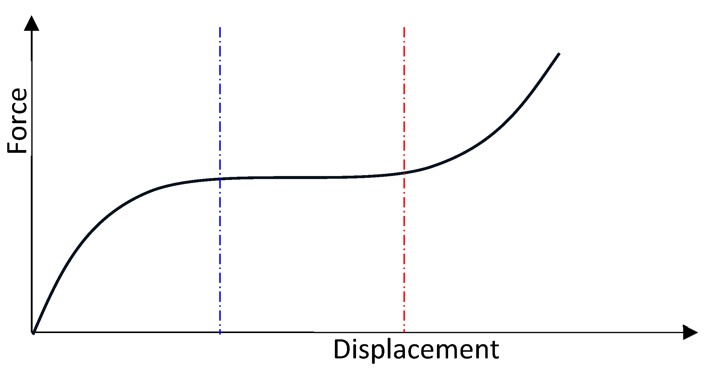
Figure 2.
Kresling unit cell [23].
Figure 2.
Kresling unit cell [23].
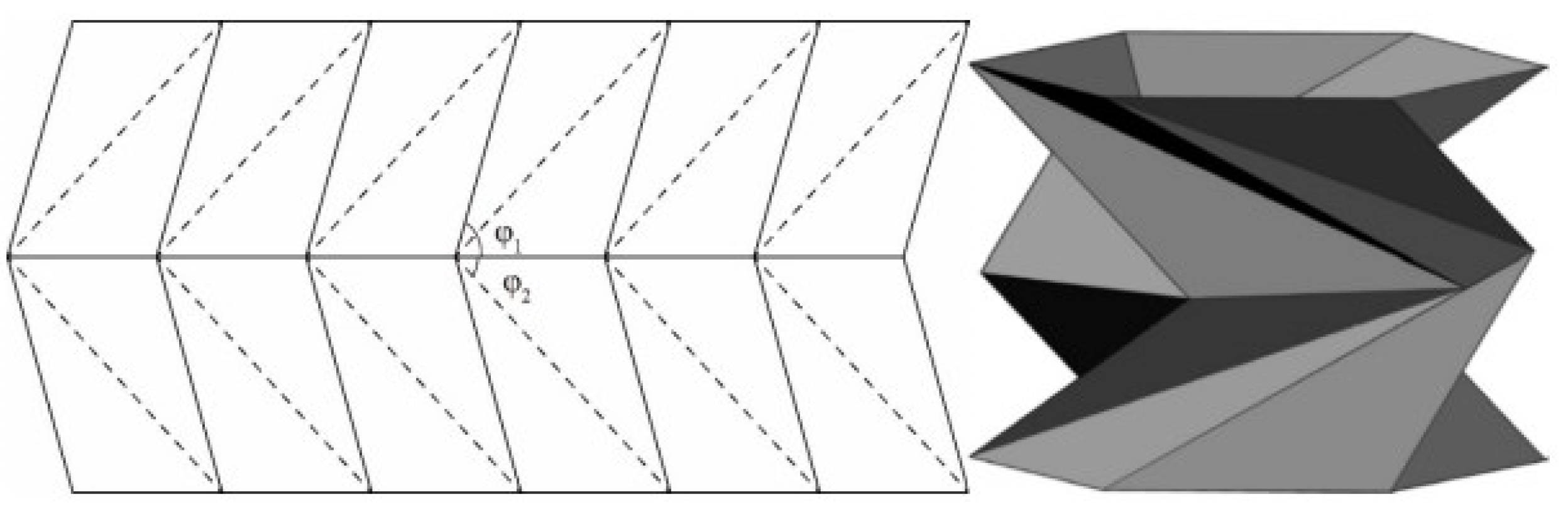
Figure 3.
Representing the geometry of all five cases.
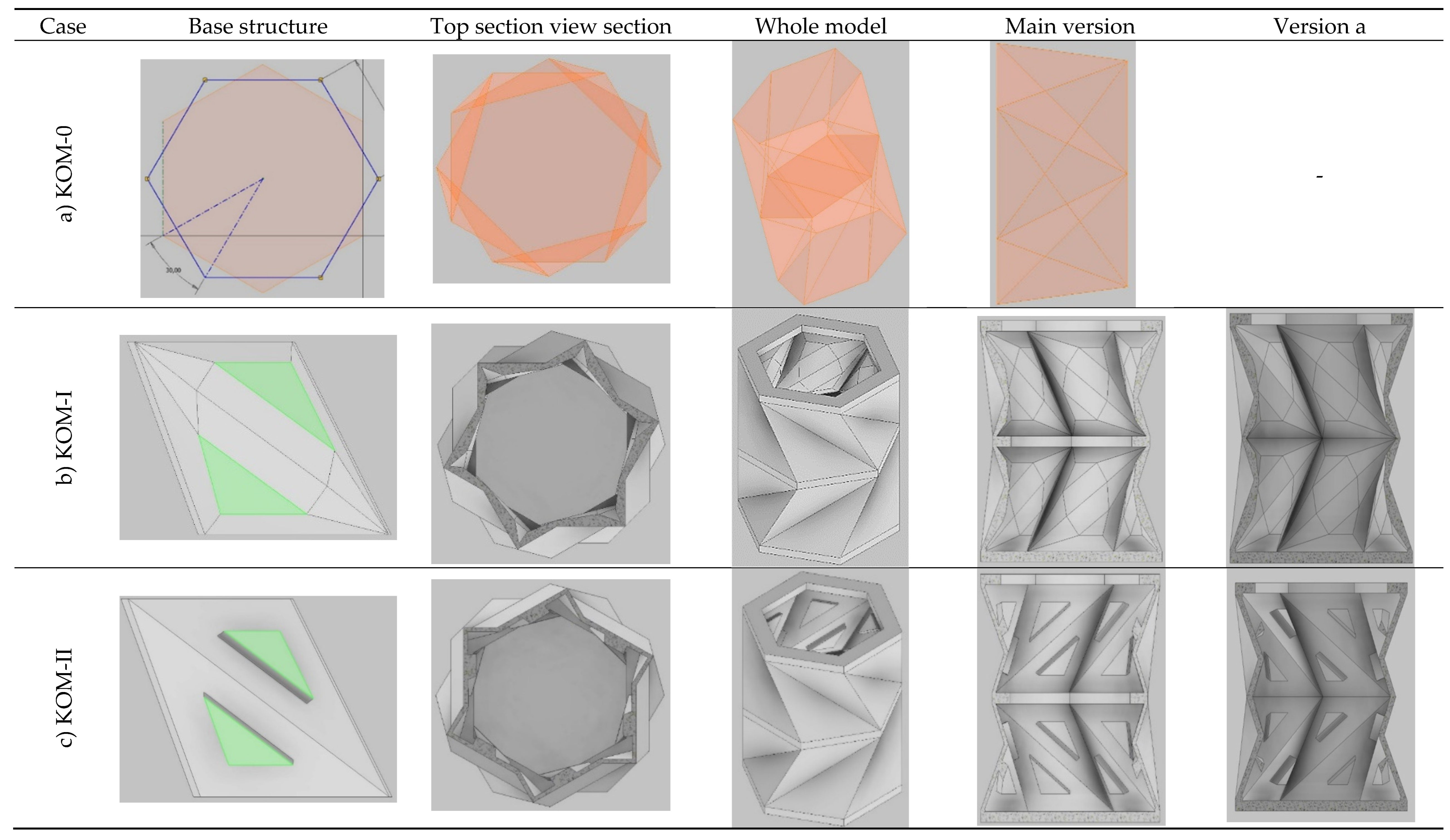
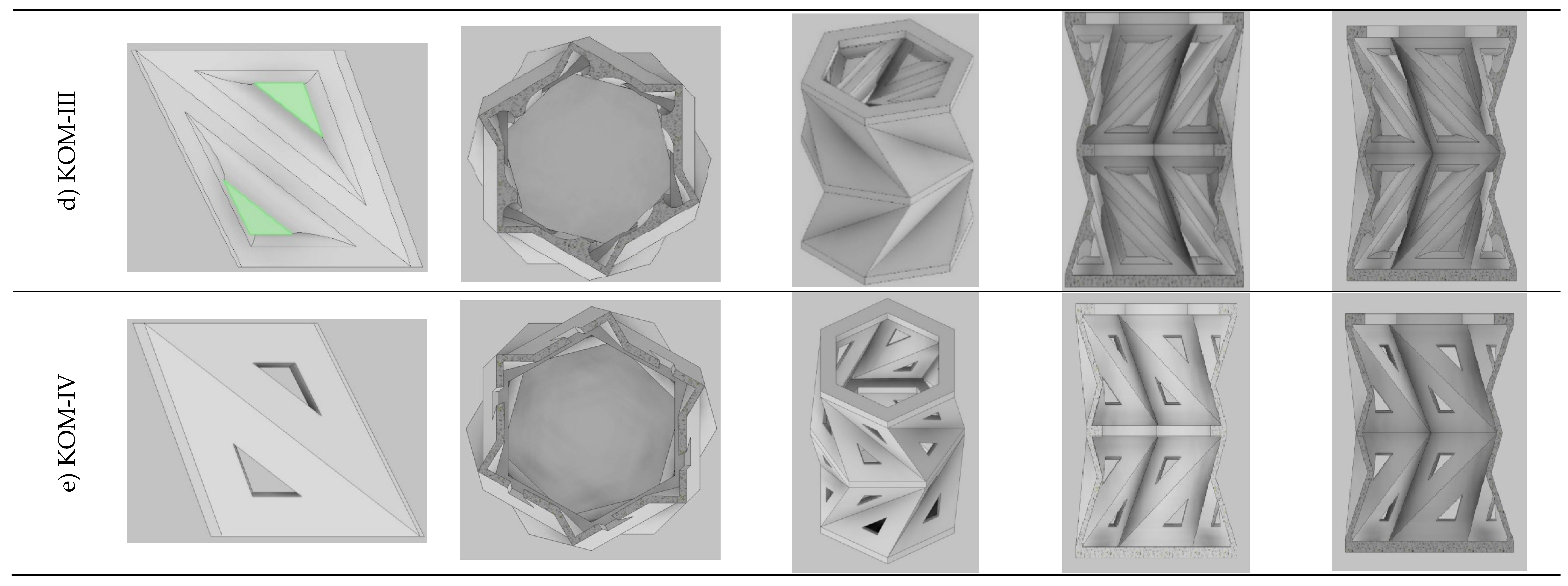
Figure 4.
Elements for meshing the geometries.
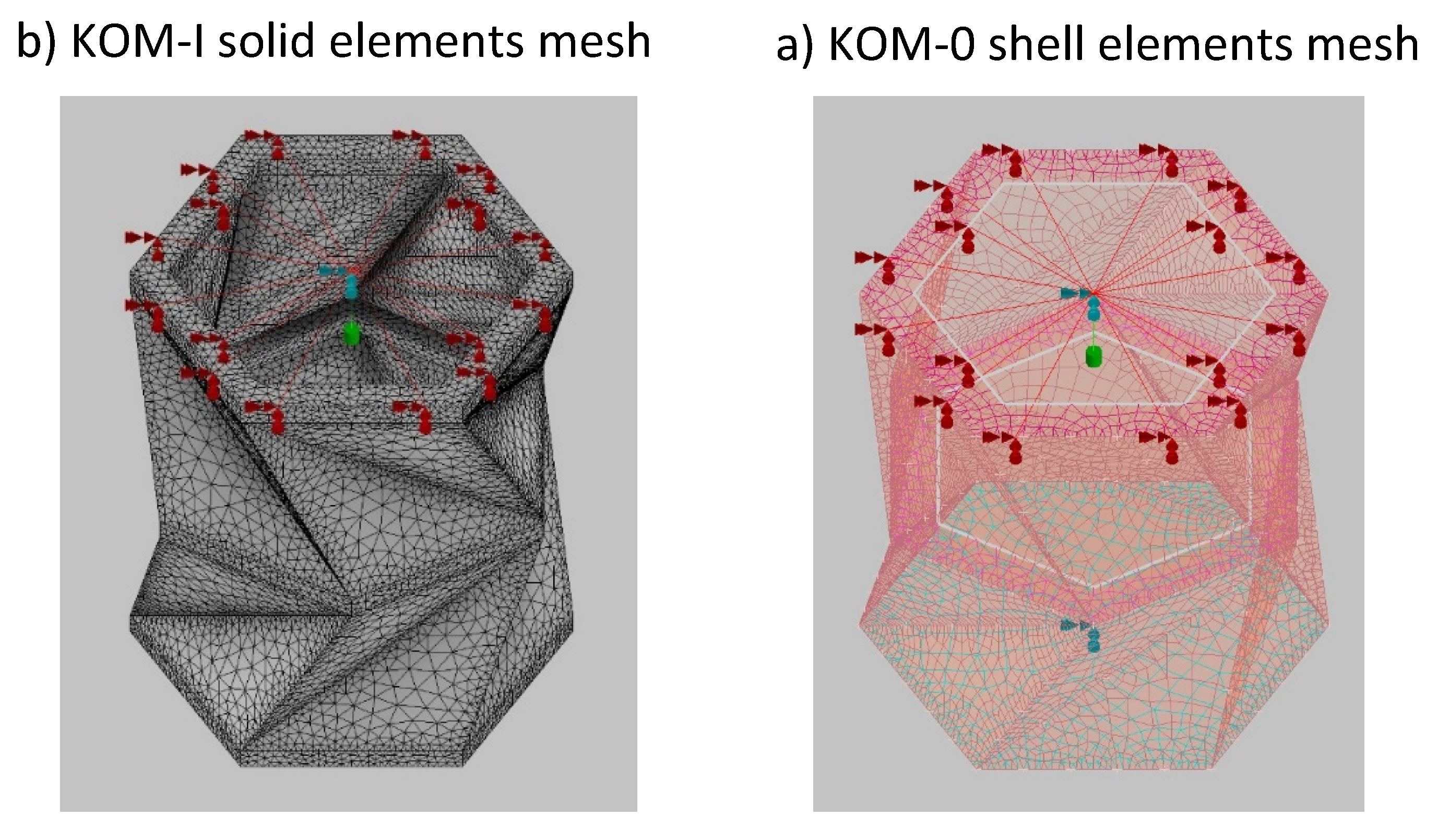
Figure 5.
Element selection for FEA; ▬ shell element; ▬ solid element.
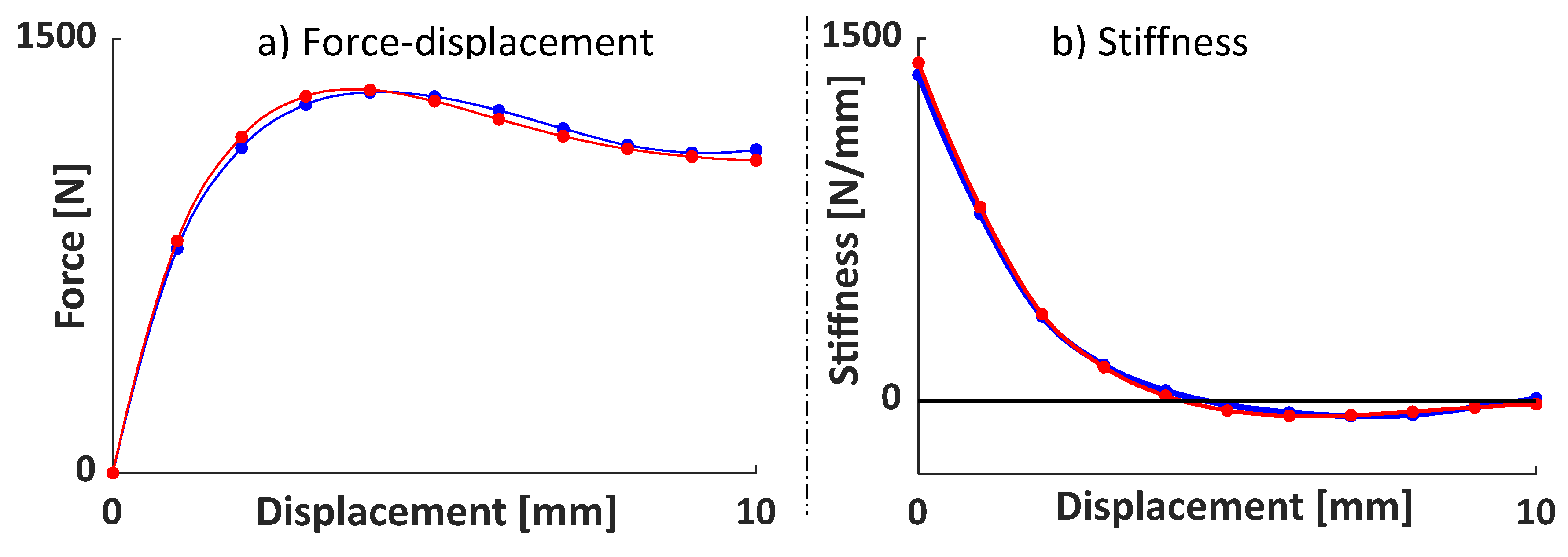
Figure 6.
Comparing all eight cases in terms of a) force-displacement, and b) stiffness ▬ KOM-I; ▬ ● ▬ KOM-Ia; ▬ KOM-II; ▬ ● ▬ KOM-IIa; ▬ KOM-III; ▬ ● ▬ KOM-IIIa; ▬ KOM-IV; ▬ ● ▬ KOM-Iva.
Figure 6.
Comparing all eight cases in terms of a) force-displacement, and b) stiffness ▬ KOM-I; ▬ ● ▬ KOM-Ia; ▬ KOM-II; ▬ ● ▬ KOM-IIa; ▬ KOM-III; ▬ ● ▬ KOM-IIIa; ▬ KOM-IV; ▬ ● ▬ KOM-Iva.
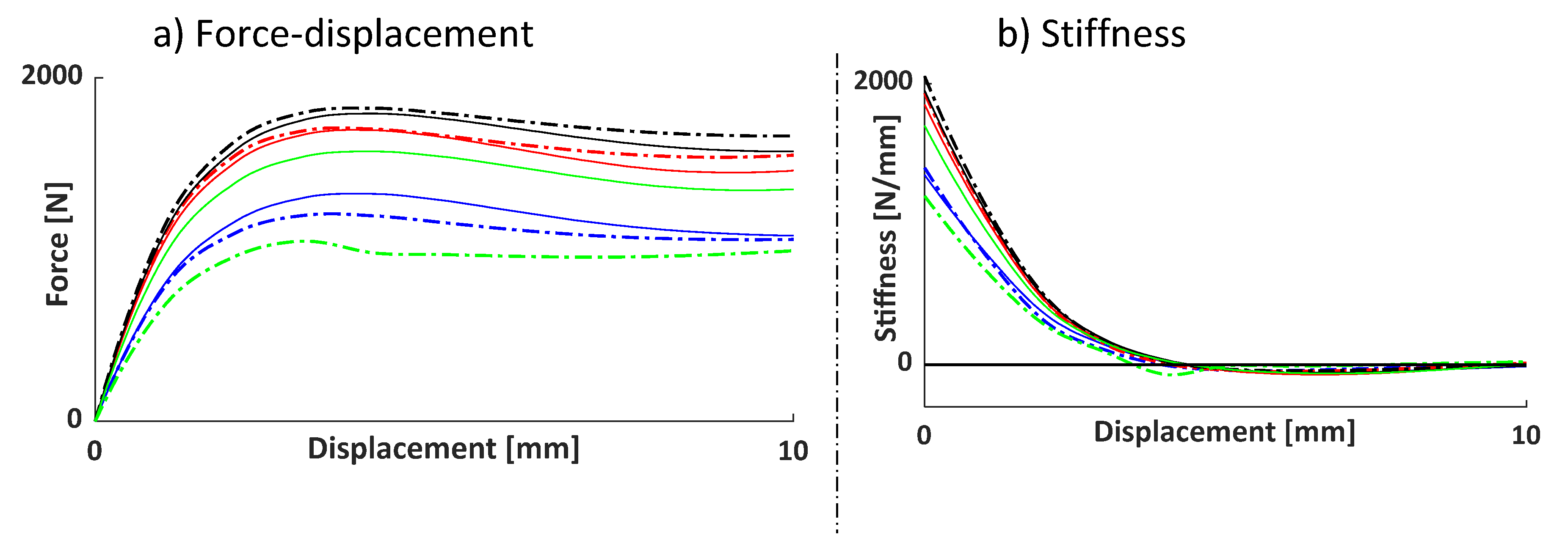
Figure 7.
Strain analysis simulation parameters.
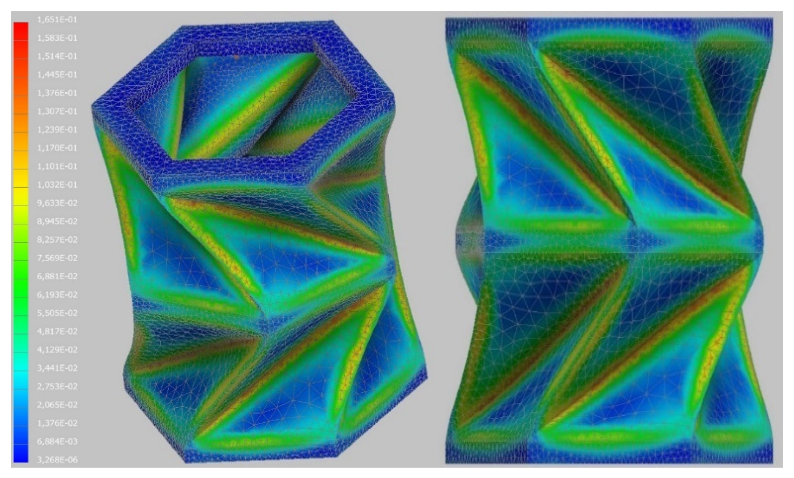
Figure 8.
a scheme of the middle plane shift angle shift angle.
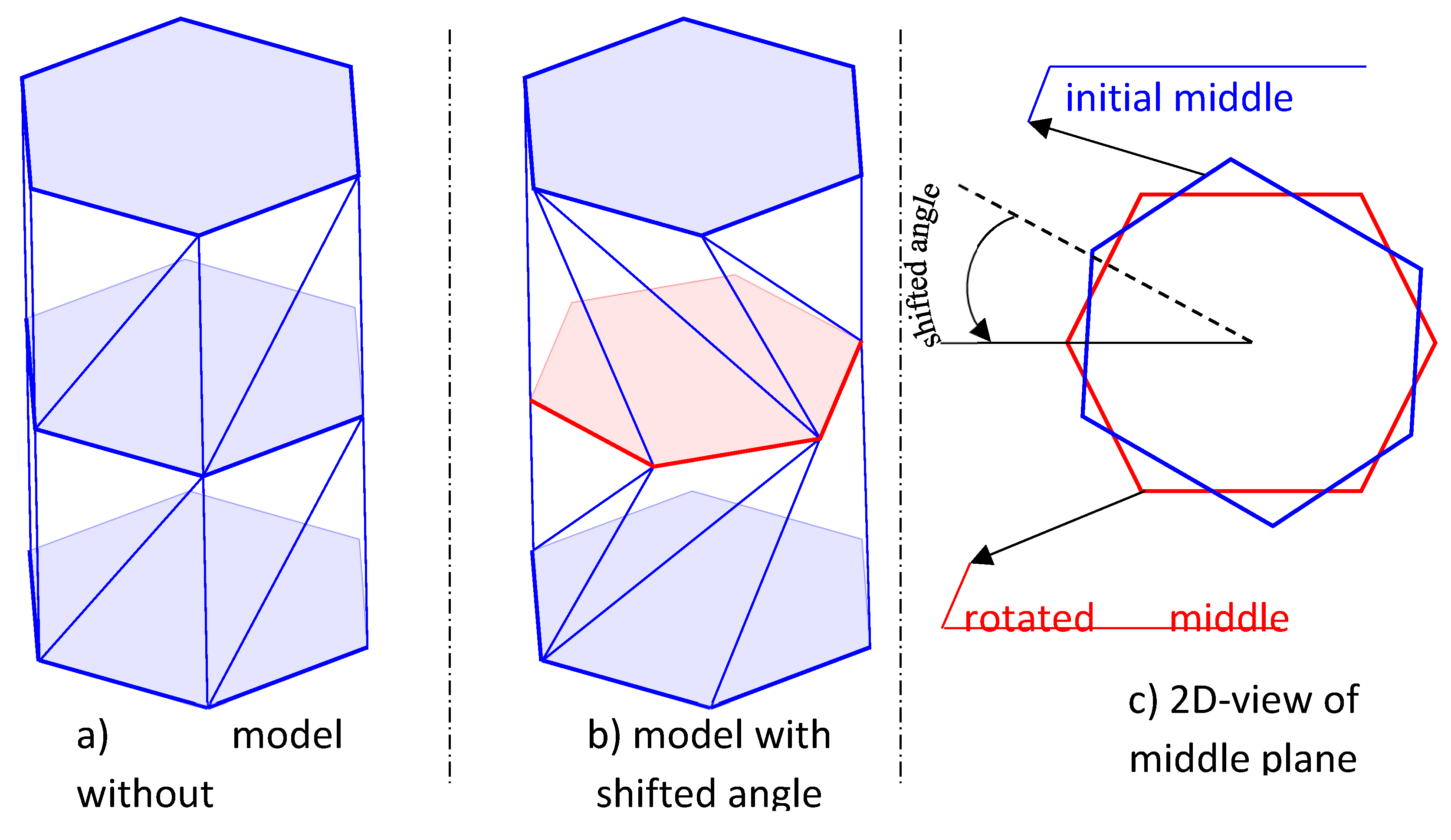
Figure 9.
Evaluating the effect of the angular shift: ▬ ; ▬ ; ▬ ; ▬ .
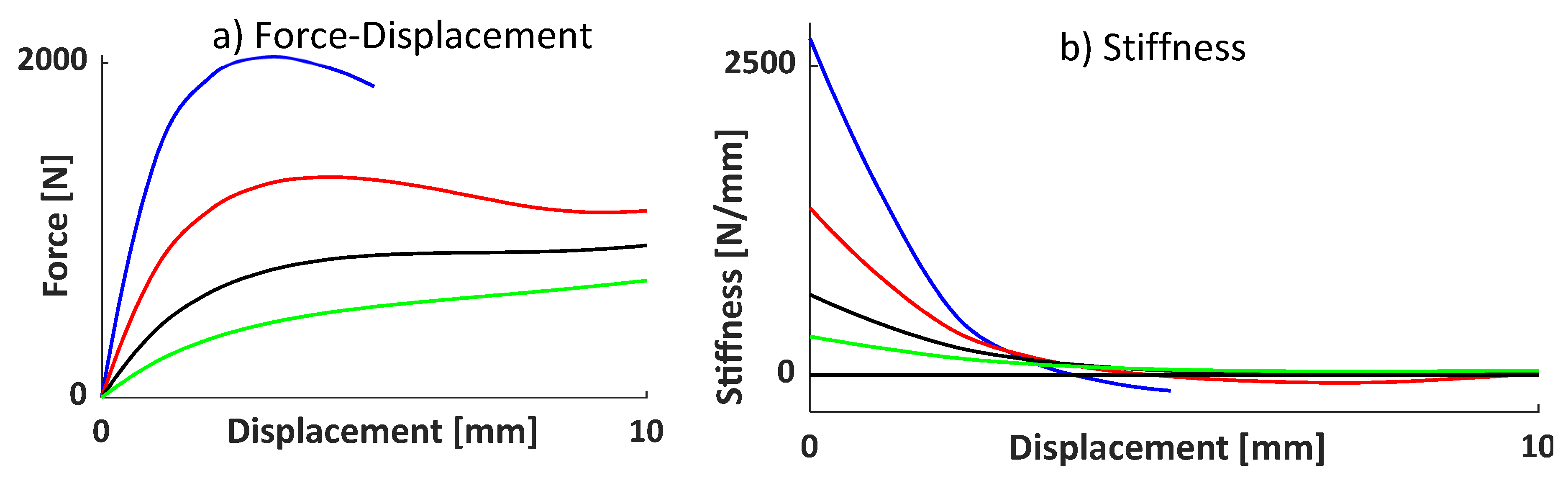
Figure 10.
a scheme where the distance between middle and base planes are illustrated.
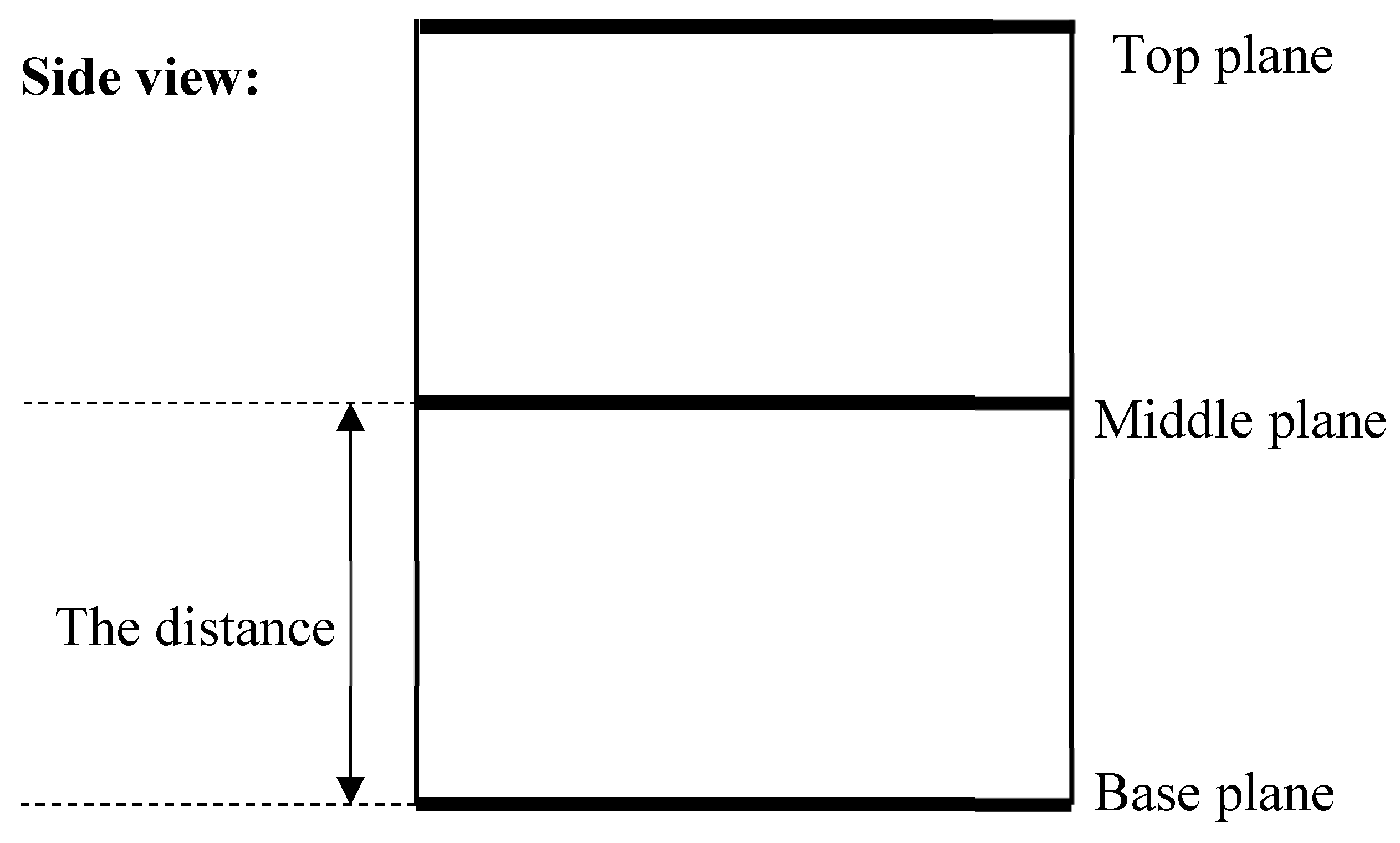
Figure 11.
Evaluating the effect of middle plane height: ▬ ; ▬ ; ▬ ; ▬ ; ▬
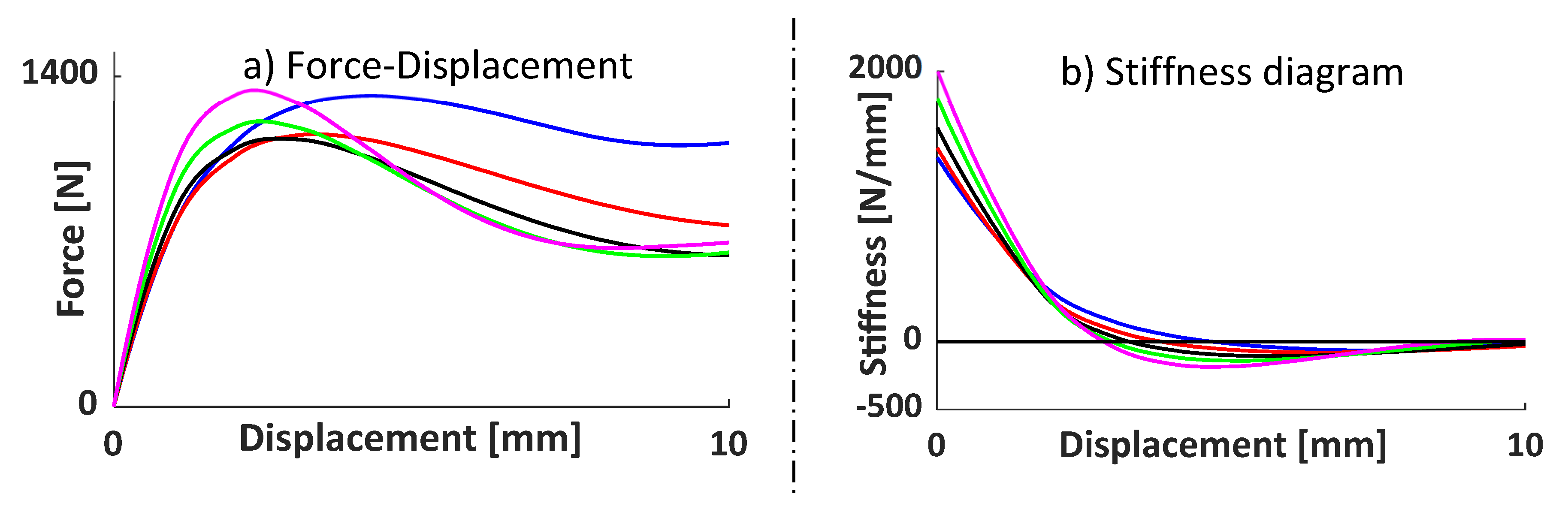
Figure 12.
a scheme of the base length.
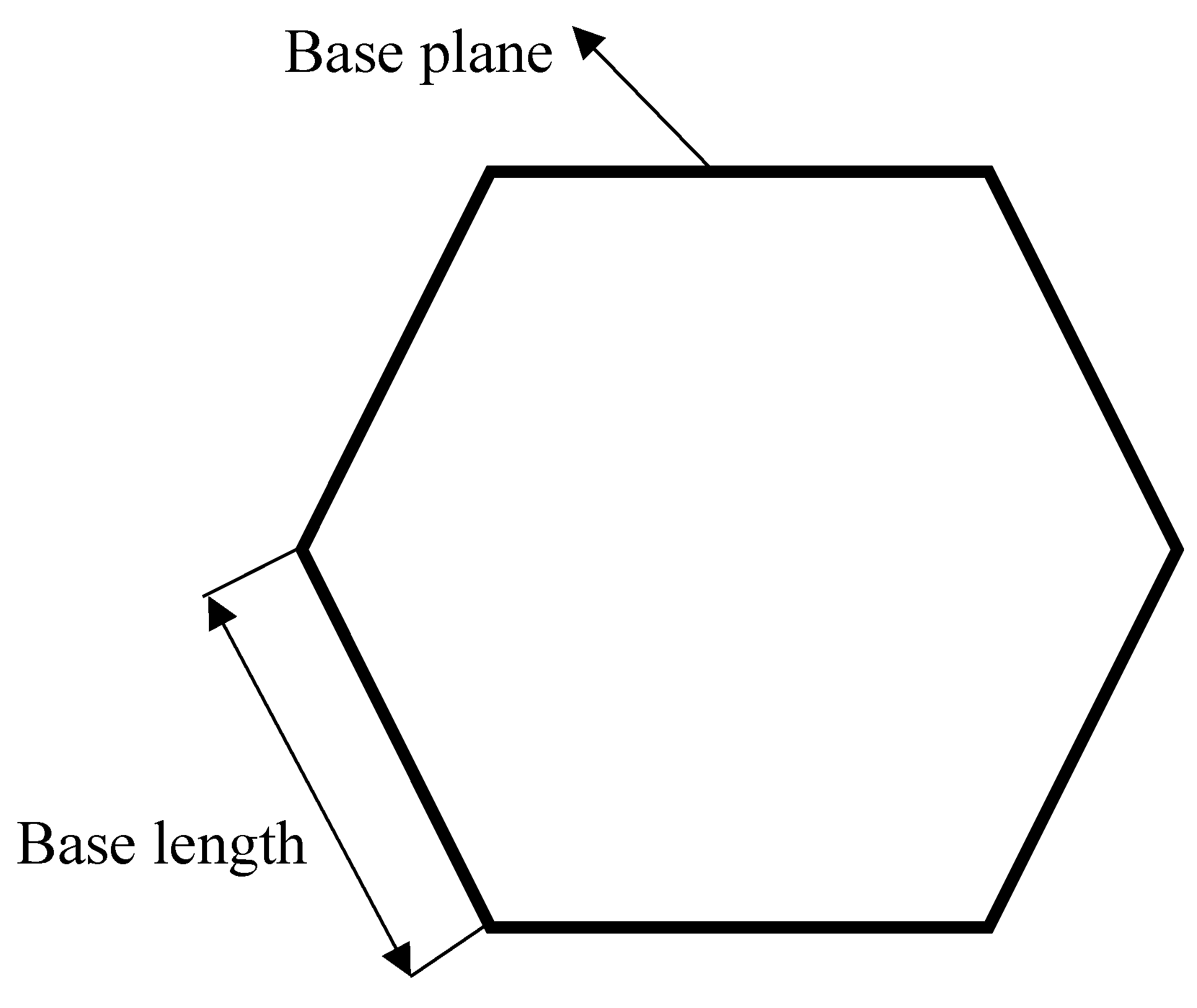
Figure 13.
Evaluating the effect of base length, ; ▬ ; ▬ ; ▬ ; ▬ ; ▬ ; ▬ .

Figure 14.
Evaluating the effect of base length, ; ▬ ; ▬ ; ▬ ; ▬ ; ▬ .
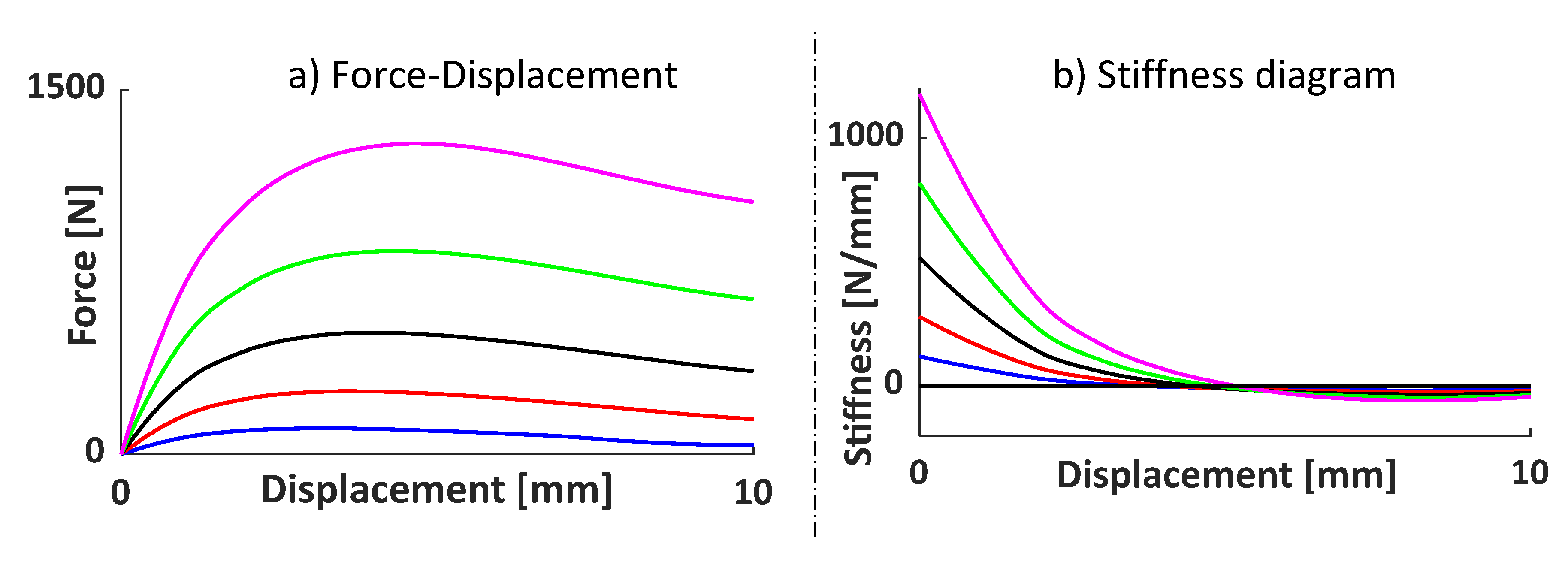
Figure 15.
KOM Multibody model.
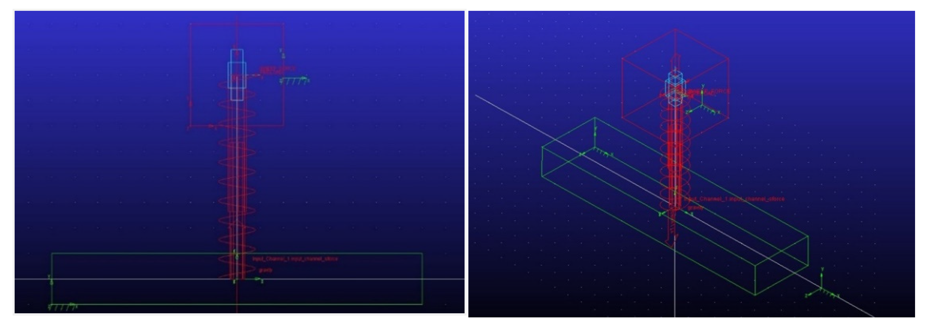
Figure 16.
FEA for KOM-IIb in the compression stroke: a) Force-Displacement, b) Stiffness diagram.

Figure 17.
Working regions for the compression stroke.
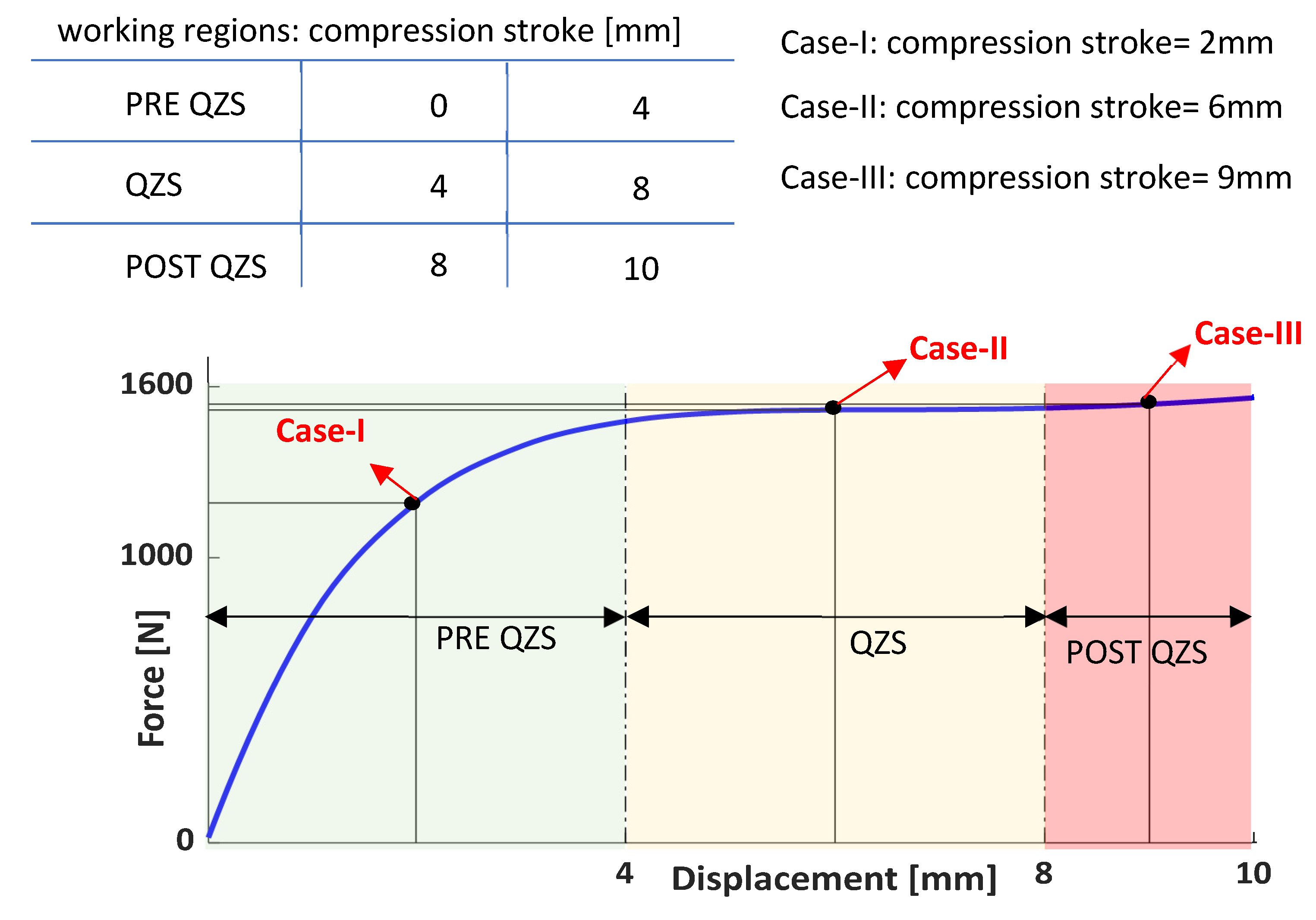
Figure 18.
Magnitude and Phase FRF comparison.
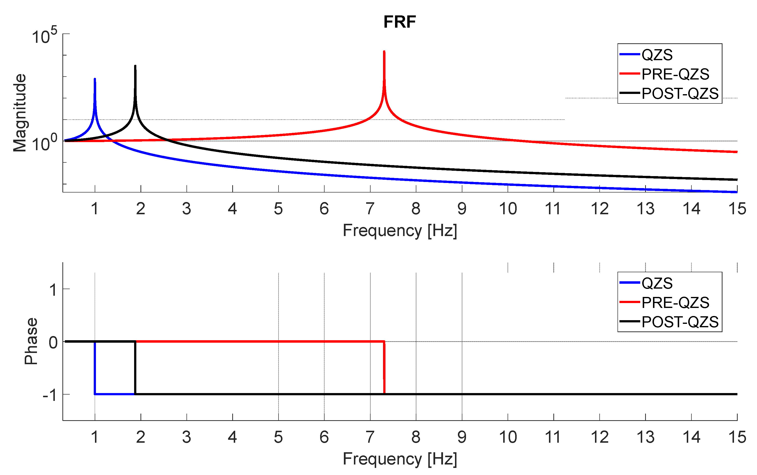
Figure 19.
the KOM-III models under compressive load (numerical results) ▬ KOM-III.1; ▬ KOM-III.2; ▬ KOM-III.3; ▬ KOM-III.4; ▬ KOM-III.5; ▬ KOM-III.6; ▬ KOM-III.7; ▬ KOM-III.8.
Figure 19.
the KOM-III models under compressive load (numerical results) ▬ KOM-III.1; ▬ KOM-III.2; ▬ KOM-III.3; ▬ KOM-III.4; ▬ KOM-III.5; ▬ KOM-III.6; ▬ KOM-III.7; ▬ KOM-III.8.
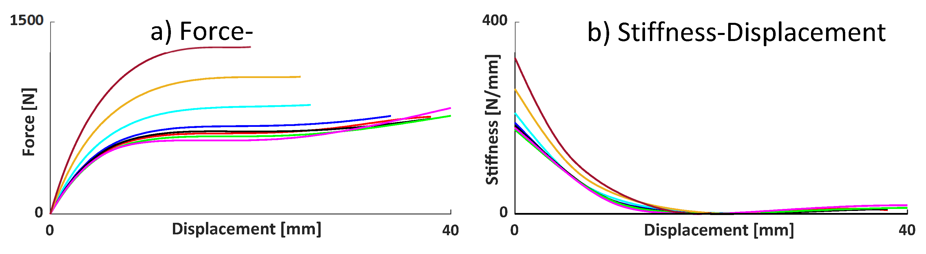
Figure 20.
KOM under compressive load for the three different materials by means of FEA.
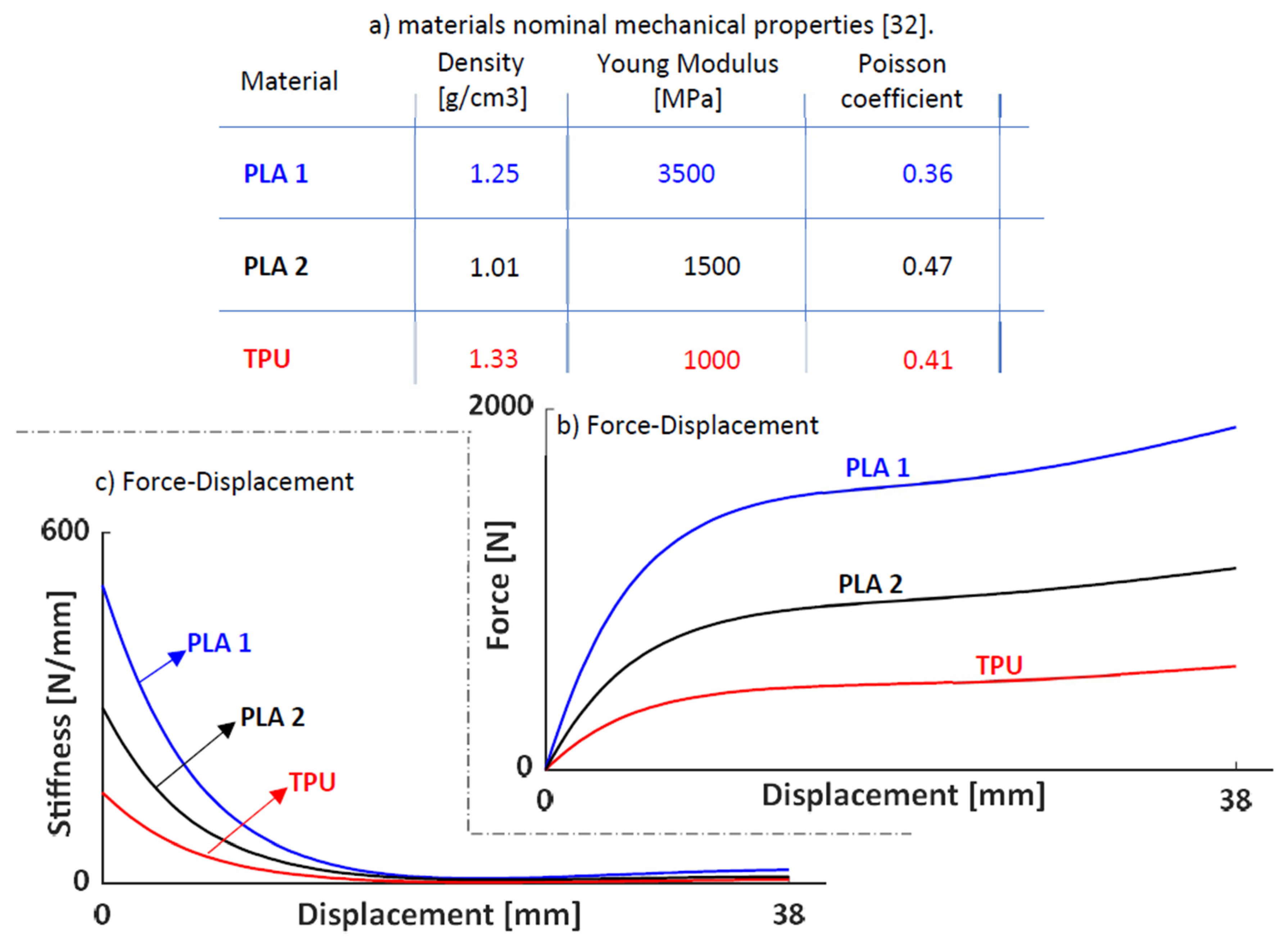
Figure 21.
KOM-III.3 prototype.
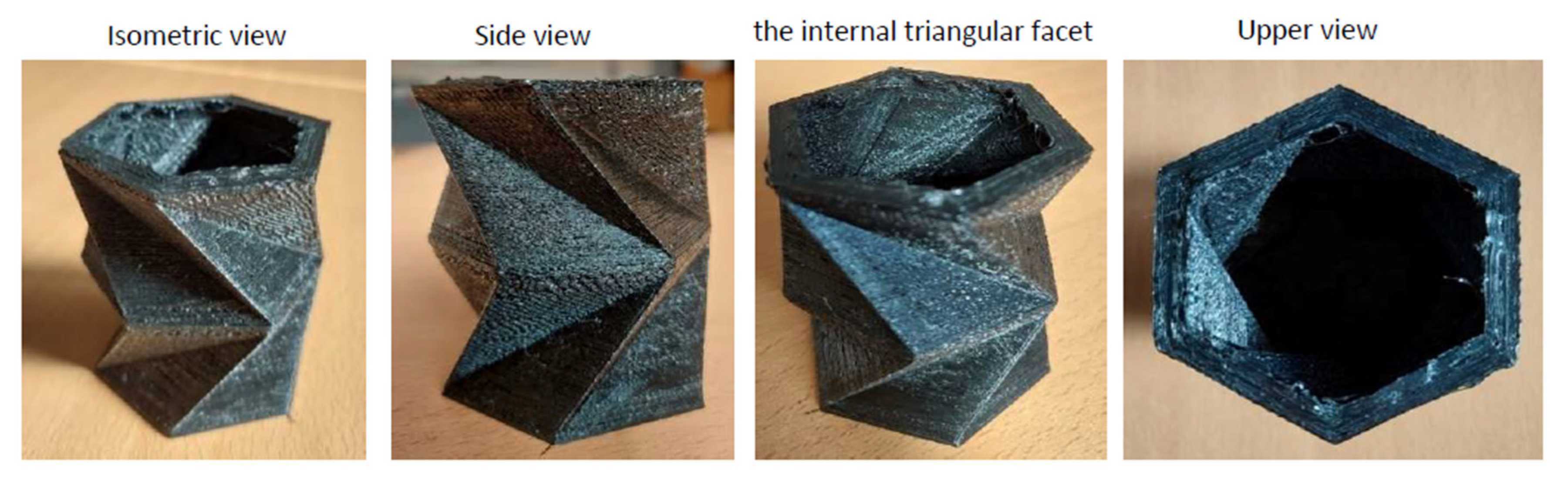
Figure 22.
Compressive test setup.
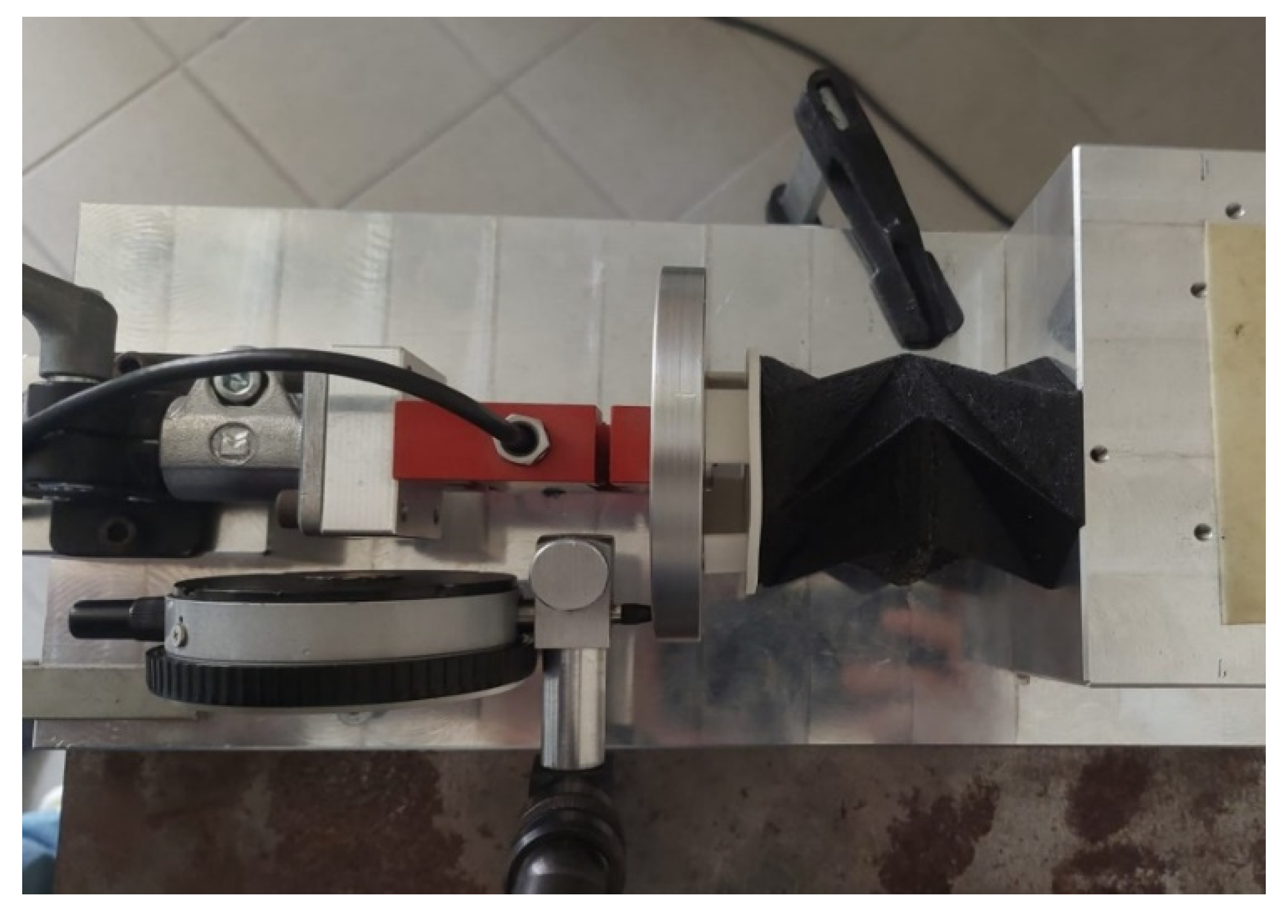
Figure 23.
Experimental results: a) Force, b) Average Force, c) Stiffness ▬ try-1; ▬ try-2; ▬ try-3; ▬ try-4; ▬ try-5; ▬ try-6.
Figure 23.
Experimental results: a) Force, b) Average Force, c) Stiffness ▬ try-1; ▬ try-2; ▬ try-3; ▬ try-4; ▬ try-5; ▬ try-6.
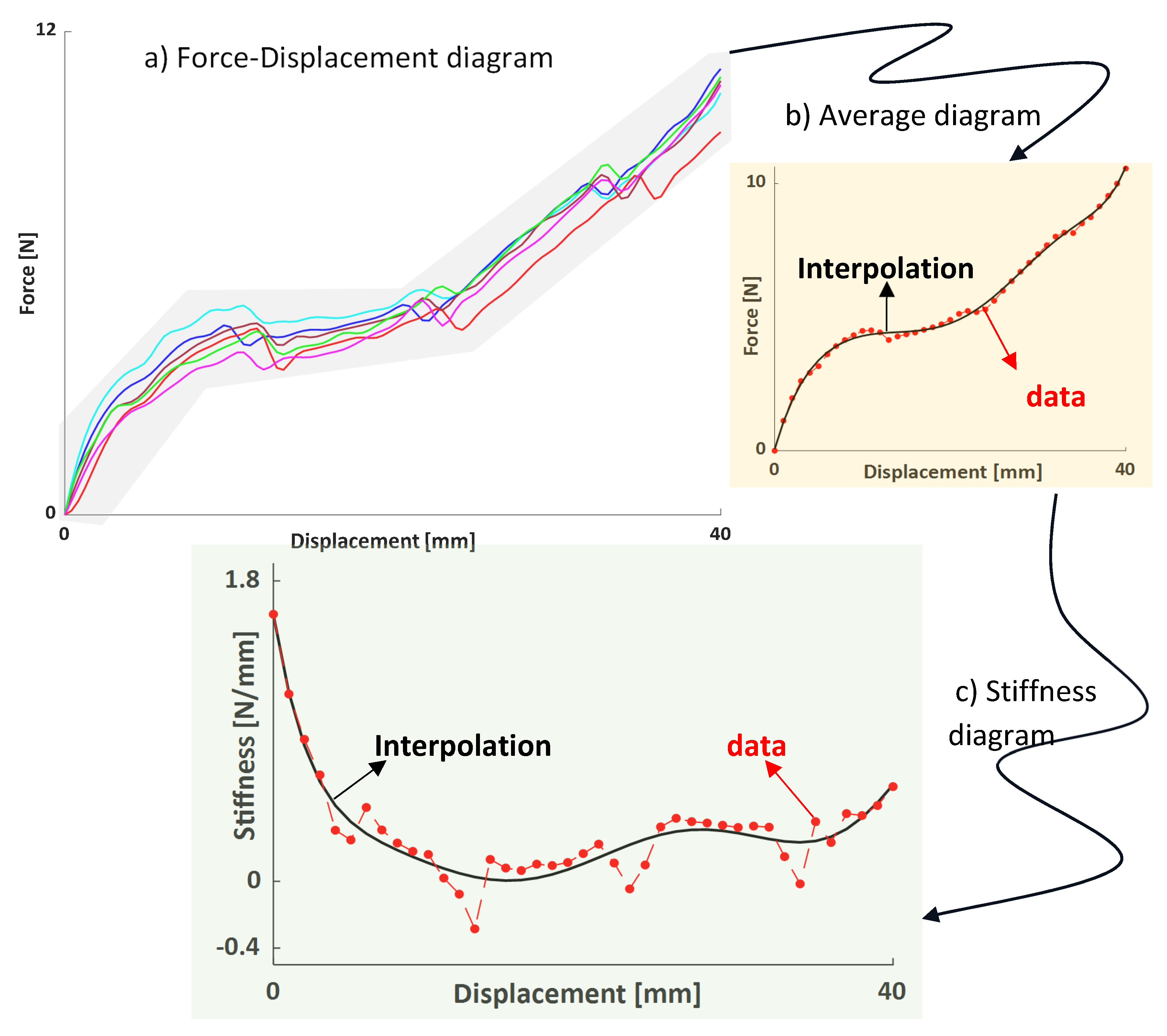
Figure 24.
Simulation results Force – Displacement at different E values ▬ ; ▬ ; ▬ ; ▬ ; ▬ ; ▬ ; ▬ ; ▬ Exp. Data.
Figure 24.
Simulation results Force – Displacement at different E values ▬ ; ▬ ; ▬ ; ▬ ; ▬ ; ▬ ; ▬ ; ▬ Exp. Data.
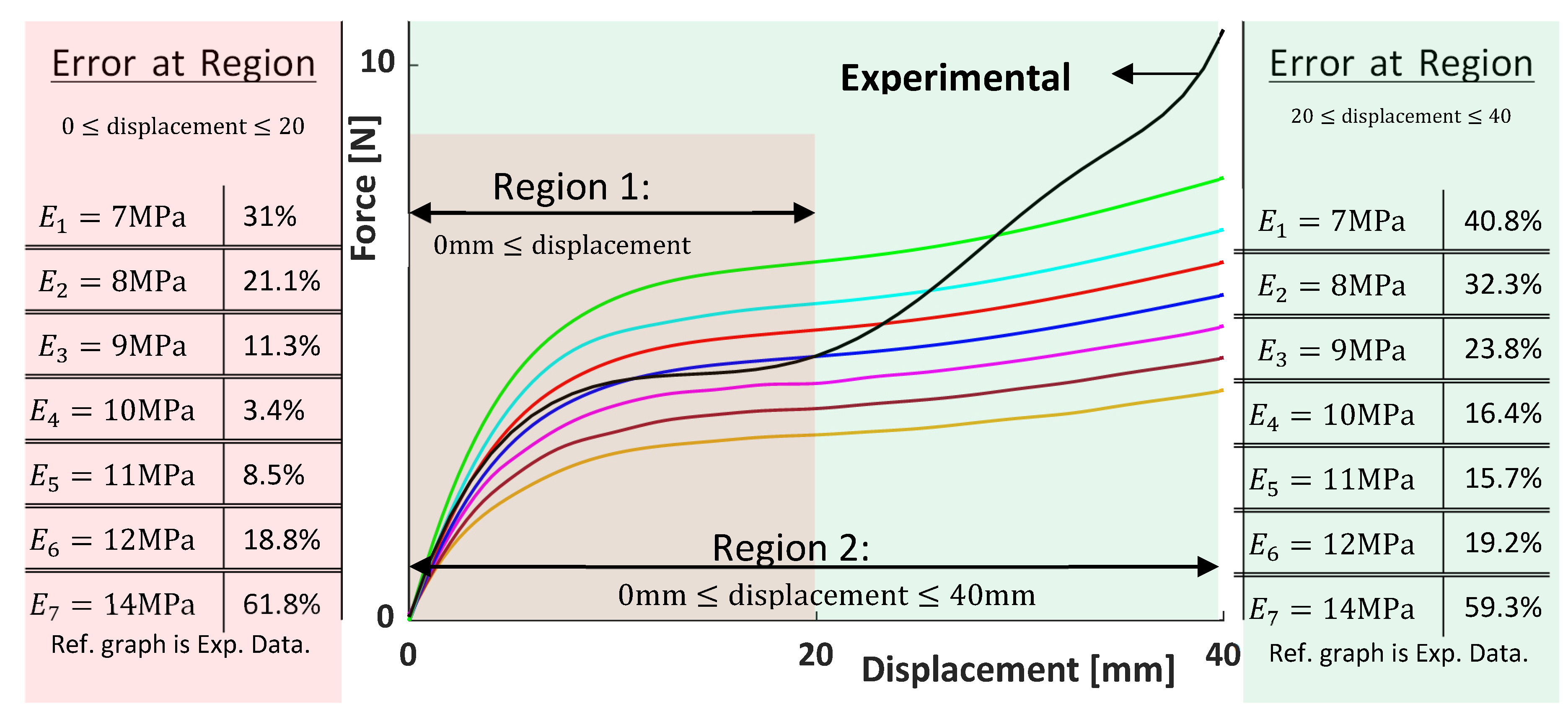
Figure 25.
comparison between a) Force-Displacement and b) Stiffness-Displacement characteristics: ▬ Experimental results; ▬ FEA results.
Figure 25.
comparison between a) Force-Displacement and b) Stiffness-Displacement characteristics: ▬ Experimental results; ▬ FEA results.
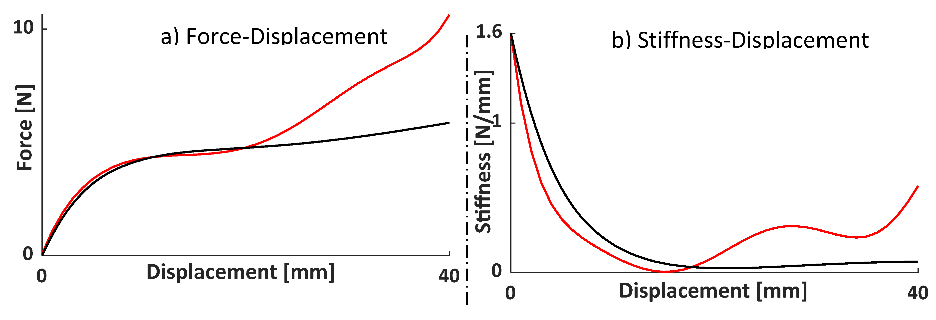
Figure 26.
FRF comparison between multibody model based on FEM and experimental stiffness.
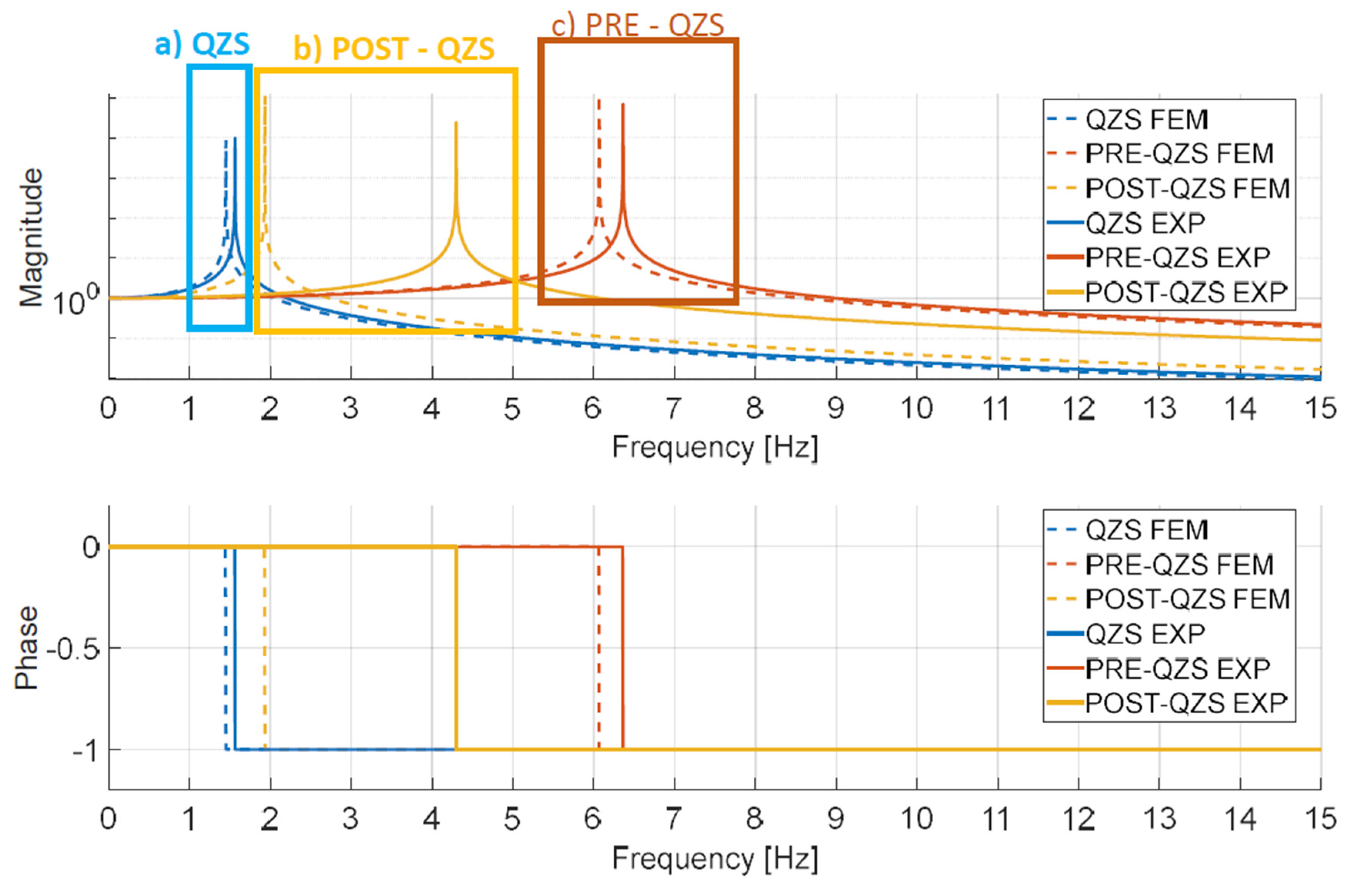

Table 1.
KOM surface model parameters.
| KOM-0 | KOM-I | KOM-II | KOM-III | |
| R [mm] | 10 | 10 | 10 | 10 |
| a0 [mm] | 10 | 10 | 10 | 10 |
| H [mm] | 10 | 10 | 10 | 10 |
| Φ start [deg] | 30 | 30 | 30 | 30 |
| Core triangle distance from edges [mm] | 0 | 2 | 2 | 2 |
| Core triangle extrusion thickness [mm] | 0 | 1 | 0.5 | 0.5 |
| Crease thickness [mm] | 0 | 0.5 | 0.5 | 0.5 |
| Base, middle and top plane thickness [mm] | 0 | 1 | 1 | 1 |
| Fillet | - | - | - | ok |
Table 2.
PLA nominal mechanical properties [27].
Table 2.
PLA nominal mechanical properties [27].
| Solid density [g/cm3] | 1.252 |
| Melt density [g/cm3] | 1.073 |
| Tensile strength [MPa] | 59 |
| Elastic modulus [MPa] | 3500 |
| Shear modulus [MPa] | 1287 |
Table 3.
FEM simulation parameters.
| Starting height [mm] | 23 |
| Compression stroke [mm] | 10 |
| Overall mesh size [mm] | 1 |
| Mesh refinement size [mm] | 0.25 |
Table 4.
FEM simulation parameters for the strain analysis.
| Starting height [mm] | 23 |
| Compression stroke [mm] | 3 |
| Overall mesh size [mm] | 1 |
| Mesh refinement size [mm] | 0.25 |
Table 5.
simulation parameters for analyzing the effects of the middle plane shift angle.
| Starting height [mm] | 23 |
| Compression stroke [mm] | 10 |
| Overall mesh size [mm] | 1 |
| Mesh refinement size [mm] | 0.25 |
| Elements type | Shell |
| Facets thickness [mm] | 0.5 |
Table 6.
KOM-IIb model parameters.
| R [mm] | 10 |
| a0 [mm] | 10 |
| H [mm] | 10 |
| Φ [deg] | 38 |
| Core triangle distance from edges [mm] | 1.5 |
| Side triangles thickness [mm] | 0.5 |
| Core triangle extrusion thickness [mm] | 1 |
| Base, middle and top plane thickness [mm] | 1 |
Table 7.
QZS region simulation parameters.
| Name | Case-I | Case-II | Case-III |
| Damping ratio | 0 | 0 | 0 |
| Stiffness (FEM data) [N/mm] | 404.03 | 7.7 | 13.56 |
| Natural frequency (FEM data) [Hz] | 8.132 | 1.123 | 1.490 |
| Starting frequency [Hz] | 0.3 | 0.3 | 0.3 |
| Ending frequency [Hz] | 15 | 5 | 5 |
| Sweep time steps | |||
| Preload [N] | 325.95 | - | 19.87 |
Table 8.
geometric parameters of the different models based on KOM-III.
| Model name | R [mm] | a0 [mm] | h [mm] | Φ [deg] | Overall height [mm] |
| KOM-III.1 | 30 | 30 | 25 | 40° | 56 |
| KOM-III.2 | 30 | 30 | 30 | 42.5° | 66 |
| KOM-III.3 | 30 | 30 | 33 | 43.5° | 72 |
| KOM-III.4 | 30 | 30 | 33 | 42° | 72 |
| KOM-III.5 | 30 | 30 | 35 | 43° | 76 |
| KOM-III.6 | 30 | 30 | 40 | 43.5° | 86 |
| KOM-III.7 | 30 | 30 | 20 | 35° | 46 |
| KOM-III.8 | 30 | 30 | 15 | 31.5° | 36 |
Table 9.
KOM Prototype working regions.
| Name | From | To |
| PRE QZS [mm] | 0 | 10 |
| QZS [mm] | 10 | 20 |
| POST QZS [mm] | 20 | 40 |
Table 10.
Comparison between Experimental and FEM properties.
| Name | Exp | FEM | Error |
| Loading mass [kg] | 0.4729 | 0.4783 | 1.1% |
| Natural frequency at QZS [Hz] | 1.5594 | 1.4499 | 7.0% |
| Natural frequency at PRE-QZS [Hz] | 6.3606 | 6.0676 | 4.6% |
| Preload for PRE-QZS [N] | 2.3734 | 2.6067 | 9.8% |
| Natural frequency at POST-QZS [Hz] | 4.2979 | 1.9308 | 55.0% |
| Preload for POST-QZS [N] | 4.8094 | 0.9564 | 80.1% |
Disclaimer/Publisher’s Note: The statements, opinions and data contained in all publications are solely those of the individual author(s) and contributor(s) and not of MDPI and/or the editor(s). MDPI and/or the editor(s) disclaim responsibility for any injury to people or property resulting from any ideas, methods, instructions or products referred to in the content. |
© 2024 by the authors. Licensee MDPI, Basel, Switzerland. This article is an open access article distributed under the terms and conditions of the Creative Commons Attribution (CC BY) license (http://creativecommons.org/licenses/by/4.0/).
Copyright: This open access article is published under a Creative Commons CC BY 4.0 license, which permit the free download, distribution, and reuse, provided that the author and preprint are cited in any reuse.