
Submitted:
20 September 2024
Posted:
23 September 2024
You are already at the latest version
Abstract
In this paper we have investigated the driven quintic Duffing equa- tion. Using some analysis technique, we are able to predict the number of limit cycles around the equilibrium and to develop a theoretical ap- proach to chaos transition in damped driven systems.
Keywords:
Homoclinic orbits
; chaos theory
; duffing equation
; Hamiltonian
AMS (MOS) Subject Classifications: 82C80, 91B62, 92C55, 11xx
1. Introduction
The Duffing equation is an example of a dynamical system that exhibits chaotic behaviour [1].The equation is given by :
where the (unknown) function is the displacement at time t. The damping factor controls the size of the damping, the controls the size of the stiffness and the controls the amount of nonlinearity in the restoring force. If , the Duffing equation describes a damped and driven simple harmonic oscillator. The quantity controls the amplitude of the periodic driving force. If , we have a system without driving force. The quantity controls the frequency of the periodic driving force. [6]
2. Homoclinic Orbits in the Unperturbed System
For the unperturbed system with fractional order displacement, when , the differential Equation (2) simplifies to
Let
Equilibrium points for are :
Define
The energy function for (3) is
where K is the energy constant dependent on the initial amplitude and initial velocity :
Dependently on K, the level sets are different. For all of them it is common that they form closed periodic orbits which surround the fixed points or or all the three fixed points and . The boundary between these two groups of orbits corresponds to , when
The level set
is composed of two homoclinic orbits
which connect the fixed hyperbolic saddle point to itself and contain the stable and unstable manifolds. The functions may be evaluated using formulas of the two following homoclinic orbits :
and
see Figure 1
The homoclinic orbit separates the phase plane into two areas.([3,4]) Inside the separatrix curve the orbits are around one of the centers, and outside the separatrix curve the orbits surround both the centers and the saddle point. Physically it means that for certain initial conditions the oscillations are around one steady-state position, and for others around all the steady- state solutions (two stable and an unstable).[5]
For and in 2 the system become perturbed , let us treat some chaotic behavior of 2 for some values of , , , and .it is known that the Duffing oscillator describes the motion of a classical particle in a double well potential such that the potential is given by , is ploted in Figure 2
We choose the units of length so that the minima are at , and the units of energy so that the depth of each well is at . We may consider the force .As usual we solve the second order differential equation by expressing it as two first order differential equations:
,where we set the mass equal to unity. Because of energy conservation ([3,7,8]), one can clearly never get chaos from the motion of a single degree of freedom. We therefore add both a driving force and damping, in order to remove energy conservation. The equations of motion become:
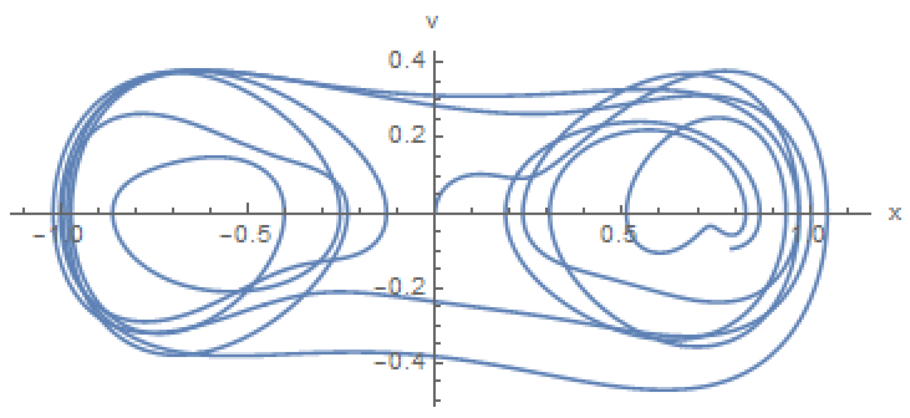
where friction coefficient, and A is the strength of the driving force which oscillates at a frequency . We will see that a transition to chaos ([9,10,11]),now occurs as the strength of the driving force is increased (The values of c must be decreasing). We will fix coefficients as: (which will be in the non-chaotic regime).We now start the particle off at rest at the origin and integrate the equations of motion. We will go up to .We obtain the following figure (see Figure 3 and Figure 4).
3. Conclusions
Control of chaos remains an area of intensive research. Reliable forecasting of the dynamics of nonlinear systems with chaotic behaviour is a challenging task. It can be solved in several ways. For example, by localizing a chaotic attractor, while obtaining a rough forecasting, or by introducing control of unstable periodic orbits embedded in a chaotic attractor, thereby making the behavior of the system predictable for given values of its parameters .
Acknowledgments
This work was partially supported by University of batna2.Algeria and universidad national de Colombia.
References
- Palmero, F. Chacon, R, Suppressing chaos in damped driven systems by non-harmonic excitations,experimental robustness against potential mismatches Nonlinear Dyn 108, 2643-2654 (2022), ,Springer.
- H.W. Haslach, Post-buckling behavior of columns with non-linear constitutive equations, In ternational Journal of Non-Linear Mechanics 20 (1982).
- S. Wiggins, Global Bifurcations and Chaos: Analy tical Me thods, Springer, New York, 1988.
- W.Y. Tseng, J. Dugundji, Nonlinear vibrations of a buckled beam under harmonic excitation, Journal of Applied Mechanics 38 (1971) 467-476.
- P. Holmes, A nonlinear oscillator with a strange attractor, Philosophical Transac tions of the Royal Society of London Series A 292 (1979) 419-448.
- P. Holmes, J. Marsden, A partial differential equation with infinitely many periodic orbits: chaotic oscillations of a forced beam, Archives for Rational,Holmes, Philip and Marsden, Jerrold E. (1981).
- Mechanics and Analysis 76 (1981) 135-166.
- G. Prathap, T., Varadan, The inelastic large deformation of beams, Journal of Applied Mechanics 43 (1976) 689-690.
- C.C. Lo, S.D. Gupta, Bending of a nonlinear rectangular beam in large deflection, Journal of Applied Mechanics 45 (1978) 213-215.
- G. Lewis, F. Monasa, Large deflections of cantilever beams of non-linear material of the Ludwick type subjected to an end moment, Journal of Non-Linear Mechanics 17 (1982) 1-6.
- H.W. Haslach, Post-buckling behavior of columns with non-linear constitutive equations, In ternational Journal of Non-Linear Mechanics 20 (1982),53-67.
Figure 1.
Homoclinic orbit.
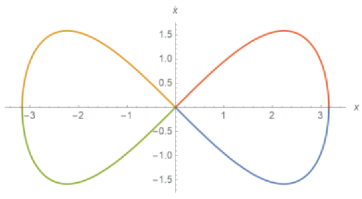
Figure 2.
Potential plot.
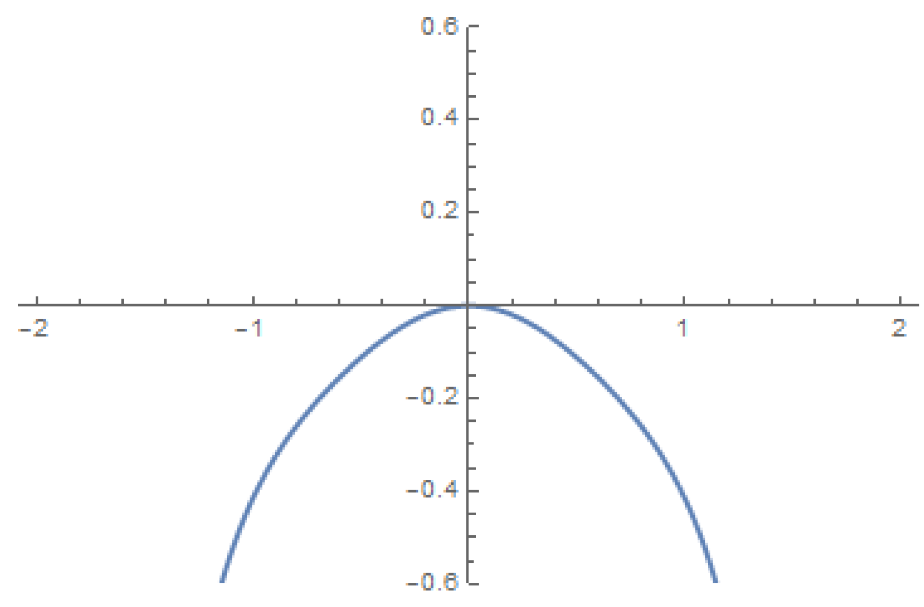
Figure 3.
Transition to chaos whenever .
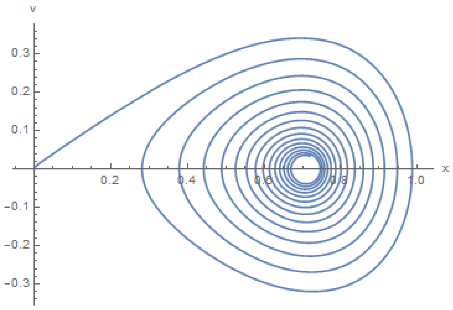
Figure 4.
Transition to chaos whenever .
Disclaimer/Publisher’s Note: The statements, opinions and data contained in all publications are solely those of the individual author(s) and contributor(s) and not of MDPI and/or the editor(s). MDPI and/or the editor(s) disclaim responsibility for any injury to people or property resulting from any ideas, methods, instructions or products referred to in the content. |
© 2024 by the authors. Licensee MDPI, Basel, Switzerland. This article is an open access article distributed under the terms and conditions of the Creative Commons Attribution (CC BY) license (https://creativecommons.org/licenses/by/4.0/).
Copyright: This open access article is published under a Creative Commons CC BY 4.0 license, which permit the free download, distribution, and reuse, provided that the author and preprint are cited in any reuse.


