

Submitted:
12 September 2024
Posted:
12 September 2024
Read the latest preprint version here
Abstract
Purpose:
Decomposition analysis of forecasting errors relating to time series generated by a 3PL logistics operator for ten distribution channels operated by the logistics operator.
Design / methodology / approach:
The studies were focused on the analysis of 10 distribution channels operated by the 3PL logistics operator who used a forecasting tool based on a modified ARIMA algorithm to prepare forecasts. In this paper, R environment was used. The studies focused on the visual analysis of forecasting error series, on the analysis of the basic parameters of the error time series distributions, on the analysis of STL decomposition and statistical tests relating to trend and seasonality.
Findings:
The forecasting error analysis indicates that there are different patterns and characteristics of errors for individual channels. The statistical test results for various channels display significant differences between forecast groups in some cases. This suggests that the forecasting tool can be more accurate for some than for other channels.
Research limitations:
Logistic operations are usually based on numerous variables which may influence forecast quality. Moreover, the absence of any information on the forecasting models and input data used may prevent complete understanding of error sources.
Value of the paper:
The studies described in this paper emphasized valuable conclusions which can be drawn from the analysis of time series forecasting errors in the context of logistic operations. The findings indicated the need for an adapted approach to forecasting for each and every channel, the importance of improving the forecasting tool and the potential to optimize the forecast accuracy by focusing on the trend and seasonality. For this reason, the analysis is an important input into the theory and practice relating to demand forecasting by logistics operators in distribution networks. The studies contribute to the works related to demand forecasting by logistics operators.
Keywords:
time series of forecasting errors
; 3PL
; logistics operator
; demand forecasting
; distribution channels
1. Introduction
The effective delivery chain management is of key importance for ensuring smooth movement of goods and services in a contemporary dynamic business environment (Davis, 1993; Fawcett et al., 2008; Towill et al., 2000). An accurate forecast plays a key role in this process, enabling organizations to make apt decisions, optimize stock levels and meet customers’ needs effectively (Babai et al., 2022; Abolghasemi et al., 2020; Hofmann and Rutschmann, 2018). Consequently, forecast accuracy is a key to improve operating effectiveness and customer satisfaction. At present, 3PL logistics operators play a crucial role in delivery chains and distribution networks (Qureshi, 2022; Kmiecik, 2022; Minashkina and Happonen, 2023; Baidoo-Baiden, 2022). Logistics operators, in particular 3PL ones, operate different channels having unique demand patterns and supply dynamics (Kmiecik and Wolny, 2022). Although the forecast models are becoming more and more advanced, their efficiency may differ depending on the channels because of inherent complexities and variability of the demand and supply characteristics. Understanding hidden patterns and behaviors relating to forecasting errors for every channel is of crucial importance for improving predictive abilities of those models.
This study is aimed at the comprehensive analysis of forecasting errors relating to time series generated by a 3PL logistics operator for ten distribution channels operated by the logistics operator. By means of the direct identification of similarities and differences of forecasting errors in different channels, the authors intend to provide practical conclusions aimed at improving forecasting models and the overall operating effectiveness which may be used for the logistics operators’ operations. The studies are aimed at filling the gap connected with the demand forecasting by logistics operators. Despite the expertise relating to the ability to implement forecasting solutions in the logistics operators’ operations (Kmiecik, 2021b; Li et al., 2022; Al. Mesfer, 2023) and the overall benefits which may be offered by the take-over of the other network participants’ forecasting function by the operator (Kmiecik, 2023) and the studies of the importance of forecasting error time series (Wolny, 2023; Yang et al., 2021; Yang et al., 2022), there have been no studies of forecasting error time series for the forecasting tools used by the logistics operators.
2. Theoretical Background
2.1. Demand Forecasting by Logistics Operators
One of more popular strategies to determine future demand is using forecasting methods to that aim. Forecasts are an input into the decision-making process relating to the supply, manufacture, deliveries and warehouse management (Alam and El Saddik, 2017) which has been stressed many times. Forecasts allow to plan production and supply of raw materials and other materials in relevant quantities and time. Thanks to that, it is possible to avoid shortages likely to result in late deliveries and in increased manufacturing costs. Forecasts allow to optimize the cost of supply and production by determining the optimum amount of raw materials and other materials as well as the delivery schedule. This leads to reduced warehousing costs and helps to avoid superfluous stock. Abholgasemi et al. (2020) (Abolghasemi et al., 2020) confirm this belief, mentioning such extra areas like demand planning, restocking, production planning and inventory control where forecasts are the grounds to make many decisions at the managerial level. A well-built forecasting system allows to plan goods flow between various production stages and between warehouses and points of sales. Thanks to that, fast and effective distribution of goods can be guaranteed and any delays and unnecessary costs can be avoided. Moreover, the forecasts are useful when implementing the assumptions of contemporary logistic concepts, e.g., mass customization (Guo et al., 2019). The forecasts also allow to adapt to the changing market conditions, including fluctuations of demand, raw material prices and also amendments to the applicable regulations. It allows to respond to market fluctuations fast and avoid unnecessary costs. Demand forecasting should allow primarily to aggregate short-term, medium-term and long-term forecasts (Kim et al., 2019). The ability to aggregate forecasts easily in different time horizons and the criterion relating to the geographic and product aggregation serves to adapt the forecasts to the requirements of individual customers. The grounds for the effective forecasting system are a well-adopted strategy of the forecast generation which includes e.g., the choice of relevant forecasting and information-flow methods. The most frequently mentioned algorithms used to forecast demand in logistic flows includes the ones based on ARIMA (Abolghasemi et al., 2020), machine learning (Chen and Lu, 2021) and neural networks (Kim et al., 2019). As it often is impossible to use highly accurate input data or adapt automatic, algorithm-based solutions to the forecasts, many forecasts are created or modified by human judgment. As stressed e.g., by Perera et al. (2019) (Perera et al., 2019), the human factor influences the forecast reliability. When forecasting, the factors of the highest impact on the forecast quality include the product history and promotion schedules (Ma et al., 2016), but also the ones relating to the distribution network coordination and its internal relations.
Forecasting starts to be associated with logistics operators. Some authors associate the operators with forecasting closely relating to the fact that the operators often forecast financial profitability of some projects (Wang et al., 2018). Oftentimes, the operators are perceived as entities forecasting demand in transport operations or cross-docking activity (Grzelak et al., 2019), although this is not an implementation approach from the perspective of this function usability for the entire distribution network. To a higher extent, it is based on the appropriate use of data found in 3PL entities. The increase in the complexity of the distribution network, in particular related to the development of omnichannel systems (Briel, 2018) is an additional stimulus for the development of forecasting systems at the level of logistics operators, which take over, in this system, the role of logistics processes coordinators (Kramarz and Kmiecik, 2022). A concept which assumes extending the logistics operators’ function is the one based on the centralized forecasting in distribution networks. Centralization can be analyzed in many aspects, e.g., transport, operations or decision making (Simoes et al., 2018). The factors which are often associated with centralization include trust and the ability to track the flows (Beikverdi and Song, 2015; Lu and Hu, 2018). In this paper, centralization will be analyzed from the perspective of implementing processes which will allow one network node to take over the decision-making function and to collect information with its subsequent appropriate analysis. The main prerequisites for centralization include (Szozda and Świerczek, 2016): the diverse nature of individual activities, which are typical for many different organizational units operating in subsequent stages of product flow, the lack of separate units responsible for coordinating processes related to managing demand for products from other processes, as well as the vertical nature of organizational structures, which intensifies the phenomenon of independent decisions regarding demand management in individual entities.
According to this concept, the logistics operator providing logistic services to a manufacturing entity and having a number of required attributes is able to take over the centralized forecasting in the distribution network. This will allow to remove the burden of the need to forecast demand from the manufacturer in the distribution network and will intensify favorable effects of the manufacturers’ specialization. The concept of the take-over of the centralized forecasting function was studied (Kmiecik, 2021a), with implementation guidelines prepared relating to the development and implementation of the forecasting model in the logistic outsourcing company (Kmiecik, 2021b). At present, the forecasting tool developed by the author has undergone an implementation pilot study in one of the international logistics operators. This solution type may have significant advantages for the entire distribution network. Given suitable conditions and attributes, the logistics operators could forecast the demand which would be a component of the broadly-taken demand management system. Demand forecasting can result in the development of the base for further activities relating to the sales, goods placement and production planning in the entire distribution network. By forecasting the demand, the logistics operators could control those components and coordinate them based on their knowledge of flow management. Another important forecasting component in the logistics operators’ structures is the use of forecasts for the operating activities. The studies reveal that the logistics operators would use the forecasting system most eagerly to support resource planning in warehousing management (Kmiecik and Wolny, 2022). However, irrespective of whether the forecasts were to help the operator coordinate flows in the entire distribution network or whether they were to serve solely the operators’ operating purposes, they would have to be characterized by high reliability. High reliability of the demand forecasts in the distribution and the warehouse is highly important for the effective management of the delivery chain and production, as it allows to plan accurately, to optimize costs, to improve service quality and increase customer satisfaction. This allows to avoid deficits resulting in delayed deliveries and cost increase, to reduce warehousing costs and avoid excessive stock, to improve service quality and ensure the entity’s continued operations. Forecast reliability can be improved based on the analysis of errors generated by the forecasting system used by the entity at present.
2.2. Forecasting Error Analysis
The forecasting error analysis is an important forecasting tool enabling to assess the adopted models’ effectiveness when forecasting future events. It consists in comparing the actual values observed in the analyzed phenomenon with the values foreseen by the adopted forecasting model. This comparison allows to identify discrepancies between the forecasts and the actual parameters and to understand the model behavior in different scenarios more thoroughly.
The basic purpose of forecasting error analysis is to estimate the forecast accuracy. To that aim, various forecasting error assessment indicators are used which help to determine the accuracy of the actual observation mapping by the forecasting model. The synthetic forecast accuracy assessment is based on averaged forecasting errors (MAE, MAPE, MSE, MASE, MdAE etc.). Two basic measures are used in this paper, i.e., MAE – Mean Absolute Error and MAPE – Mean Absolute Percentage Error.
where n – number of errors, – observed value, – predicted value.
The forecasting error measures play an important role in the forecast quality assessment. They are characterized by the general level of the forecasting model error regardless of the length of time in the future covered by the forecast, i.e., of the forecast time horizon. Those synthetic measures of forecasting errors are grounds for comparing different forecasting models and assessing their performance. They provide information on the mean deviation between the predicted and the actual values which allows to look at the overall forecast effectiveness in the context. For example, MAE indicates how much the forecast values differ from the actual ones in an average case, whereas MAPE expresses that error as an actual value percentage which helps to assess forecasts in the context of their significance for the phenomenon. The comparison of forecasting error synthetic measures may also provide further information on the error distribution asymmetry.
However, to carry out a more accurate forecast quality analysis, it is necessary to analyze a comprehensive error distribution. The values of synthetic forecasting error measures may hide various error aspects, including outliers, skewness of the distribution or other irregularities. This is why it is so important to analyze error distribution. A more detailed error analysis consists in studying the time series of forecasting errors. In such a case, the time series properties are interesting. The analysis entails primarily the answer to the question on whether the series has any regularities allowing e.g., to decompose the series into systematic constituents (seasonality, trend). Consequently, the analysis should lead to the conclusions relating to the forecasting model assessment, including the opportunity or necessity to adjust it.
3. Methods
This is a case study of two distribution networks where the logistics operator provides logistic services for a manufacturing company (Figure 1).
This is a logistic company specializing in the distribution and warehousing of goods for different entities. This company offers a broad range of logistic services, including transport, warehousing, delivery chain management, forwarding services and stock-taking processes. The operator keeps investing in cutting-edge technology and offers training to their employees to meet the market requirements and improve competitiveness. The operator operates on the international market primarily in Europe, but also outside it.
For their operating activities, the operator uses a forecasting tool fed with data from WMS (Warehouse Management System). To facilitate their warehousing activities, the operator decided that the tool would be used primarily to forecast collective releases (for all SKUs, i.e., Stock Keeping Units) for various picking methods and sales channels. Various picking methods imply diverse warehouse stock involvement in the process of the customer’s order preparation. The said forecasting tool is supplied with WMS data and is based on the modified ARIMA algorithm (Autoregressive Integrated Moving Average). ARIMA is a time series forecasting model that is commonly used in statistical analysis to understand the pattern of data over time and forecast future values based on the patterns found. ARIMA models can be used to model and forecast data that has three key characteristics: stationarity, autocorrelation, and seasonality. Stationarity refers to the property of a time series that has a constant mean and variance over time. Autocorrelation refers to the property of a time series where the values of the series at different time points are correlated with each other. Seasonality refers to the property of a time series that shows regular patterns or cycles over a fixed period of time, such as daily, weekly, or monthly (Hyndman and Athanasopoulos, 2018). The ARIMA model is built by combining the AR (Autoregressive) model, the MA (Moving Average) model, and the differencing method. The AR component models the dependence of the current value on past values of the same series, while the MA component models the dependence of the current value on past errors. The differencing method is used to remove the trend and seasonality of the series, making it stationary and easier to model (Box et al., 2015). ARIMA models are commonly used in demand forecasting because they are able to capture the complex patterns and trends often found in demand data, such as seasonality and autocorrelation. The tools employed by the operator use a commercial version of the modified ARIMA algorithm (www.cloud.google.com). That extends the capacities of the traditional ARIMA model. It is designed to handle time series which display complex patterns and it has such functionalities as the automatic detection of seasons, automatic detection of outliers and the ability to handle missing data values. The model overcomes some limitations of the traditional ARIMA model by introducing new functions (Table 1).
The discussed model is used by the logistics operator and has collected historical data concerning the forecast and actual values for ca. half a year. In this context, the forecasts were generated in a 30-day horizon with daily data updates in daily granulation. The forecast values were consistent with the managerial requirements learned during the analysis of the operator’s business needs and were based on forecasting collective values of SKU releases where the release handling was similar (forecasts for different picking methods).
The studies focused on the analysis of two distribution networks where the logistics operator providing services to the manufacturer operates. In both cases, the forecasting tool operates based on the above-mentioned assumptions and is oriented towards forecasting collective SKU releases for various picking methods. The first case (Manufacturer 1) is a distribution network where the manufacturer specializes in pharmaceutical products and their two main sales channels operated logistically by the operator include the distribution to hospital and to pharmaceutical wholesalers. In both circumstances, the forecasts referred to three picking types, e.g., picking of individual units, picking of a cardboard collective packagings and picking of shrink-wrap collective packagings. In the other distribution network, the logistics operator provides services to a manufacturer of household appliances (Manufacturer 2), for whom the forecasts are generated for two main distribution channels, i.e., e-commerce and brick-and-mortar stores, divided into four main picking methods (picking of individual units from the mezzanine, picking of individual units from the racks, picking of cardboard boxes for e-commerce and picking of cardboard boxes for brick-and-mortar stores). The general data characteristics for the individual manufacturers is presented in Table 2.
Various picking methods define different use of resources for warehousing works relating to SKU releases from specific perspectives. For this reason, accurate forecasts facilitate the components relating to resource planning in the warehouse. The paper analyses series of forecasting errors collected in the forecasting tool implemented by the logistic operator. The paper contains two research hypotheses (Figure 2).
The hypotheses are as follows:
H1.
In the forecasting errors for different picking systems, it is possible to find certain regularities allowing to decompose them in terms of seasonality and trend.
H2.
The analysis of the forecasting error series may improve the operation of the current forecasting tool in terms of the generated forecasts’ reliability.
The first hypothesis refers to the attempt at detecting the regularity of e.g., seasonality or the deterministic constituent in the series of forecasting errors relating to different picking methods. The verification of this hypothesis will provide the answer to the question of whether the forecasting tool operation has any regularities relating to the errors of the forecasts. The second hypothesis is to verify if the analysis may affect the tool operation and improve the reliability of forecasts generated by it.
The error series was analyzed in the R environment (R Core Team, 2022), including but not limited to the “forecast” package (Hyndman et al., 2023). A significance level of 0.05 was adopted for statistical inference. The error series randomness was analyzed using a “randtests” package (Caeiro F, Mateus A, 2022). The hypothesis concerning trend presence was verified using the functionalities from the “funtimes” package (Lyubchich V., Gel Y., Vishwakarma S., 2023). Seasonality was analyzed by means of the “seastest” package (Ollech D., 2021).
Additionally, H1 hypothesis was verified using the procedure described in the reference work (Wolny 2023). The systematic components of seasonality and trend were identified by means of the STL decomposition (Cleveland et al., 1990). The strength of the error seasonality and trend presence was assessed using the following measures (Wang et al., 2006):
where Tt is the smoothed trend component, St is the seasonal component and Rt is a remainder component. Equation (3) describes the strength of the trend component, whereas equation (4) the strength of the seasonal component.
The R package functionalities used for error analysis are presented in Table 3. The detailed assumptions concerning the functionalities employed are presented in the column called “Functionalities employed”. The default values for the functionality are the values of the other, non-specified, parameters.
4. Results
The first step of the analysis was the visual assessment of the forecasting error series. The visual analysis of the forecasting error time series consists in plotting those errors on the timeline. Such diagrams may reveal the existing patterns, including cyclicality, seasonality or the trend, which were not visible in the analysis of the forecast value time series. For example, if the series of forecasting errors display regular fluctuations in specific periods of time, this may suggest that the forecasting model has difficulties predicting certain seasonal patterns. The behavior of the analyzed time series is presented in Figure 3.
The visual analysis of the forecasting error times series is an important stage of the forecasting model analysis. By means of the reliable understanding of error series patterns and properties, the researchers and analysts may identify significant relationships and aspects which are worth analyzing further and in more detail. Such an approach allows to understand the forecasting error dynamics and potential model-related problems better. Following the visual analysis, it is possible to carry out a more advanced statistical analysis. Calculations of the basic parameters of the forecasting error distribution, including the mean value, standard deviation or skewness, may provide information on the error characteristics and asymmetry. Moreover, the STL decomposition (Seasonal and Trend decomposition using Loess) allows to determine the components of the trend, seasonality and the remainder which may help to identify the major sources of errors in the forecasts. Statistical hypothesis testing plays an important role in the analysis. Determination of the p-value for the tests with the hypothesis concerning the absence of any trend or seasonality allows to find out whether there are any statistically significant deviations from those assumptions. The basic numerical characteristics of the analyzed error time series are presented in Table 4.
The analysis of the forecasting error time series for different channels revealed diversified error patterns and characteristics in those channels. Some channels tend to overestimate, whether others to underestimate the forecast values. The differences of the standard deviation, coefficient of variation, skewness and kurtosis indicate diverse error variation. For every channel, the analysis of those parameters may offer valuable guidelines for further optimization and improvement of forecasting models. For Channel_01, the mean value of error is 172, whereas the median is 176, which suggests that most errors are below the mean value. However, the asymmetry coefficient value indicates that there is a poor asymmetry of error distribution. However, high standard deviation (1,095) and high value of the coefficient of variation (CV = 6.212) point to high error variation. For Channel_02, the mean error is 245, whereas the median is 507, suggesting that the models tend to underestimate the predicted values. High standard deviation (2,268) and kurtosis (11.280) indicate significant variation of the error distribution. Analyzing Channel_03, a conclusion can be drawn that the mean error is close to zero, but low median (15.5) and high standard deviation (174) indicate diverse error characteristics. Skewness is close to zero and kurtosis (4.387) proves higher value concentration than in the normal distribution (kurtosis is 0). For Channel_04, the mean error is 574, whereas the median is 297, suggesting the underestimation of the predicted values. High standard deviation (5,665) and kurtosis (2.270) indicate significant error variation and a certain degree of the analyzed values dispersion. The distribution is right-skewed. The mean error in Channel_05 is 126 and the median is 149, suggesting small value undervaluation. High standard deviation (1,017) and the coefficient of variation (8.040) indicate significant variation. The distribution is left-skewed. For Channel_06, the mean error is 25, whereas the median is 29.5, suggesting small value underestimation. Low standard deviation (52) and kurtosis (0.567) indicate relatively low variation and the distribution close to normal. The distribution is left-skewed. The mean error for Channel_07 (-1,387) and the median (-687) are negative, suggesting the tendency to overestimate the predicted values. High standard deviation (2,822) and kurtosis (-0.487) indicate significant error variation and platykurtic distribution. The distribution is left-skewed. Channel_08 is characterized by the mean error of -706 and the median -175, suggesting overestimation of the predicted values. High standard deviation (1,602) and kurtosis (-0.774) indicate certain error variation and platykurtic distribution. The distribution is left-skewed. For Channel_09, the mean error (-1,583) and the median are negative (-732), suggesting overestimation of the predicted values. High standard deviation (2,969) and kurtosis (-0.726) indicate significant error variation and platykurtic distribution. The distribution is left-skewed. For Channel_10, the mean error is -228, whereas the median is -147, suggesting value overestimation. High standard deviation (420) and kurtosis (-0.354) indicate error variation. The distribution is left-skewed.
Generally speaking, the value of the coefficient of variation (CV = Std.Dev / Mean) indicates high variation in the analyzed error distributions.
The subsequent analytical step was to analyze the forecasting error randomness. The results are presented in Table 5
The analysis of the forecasting error randomness indicates that each analyzed series can be considered random (in the sense of one of the tests used and alpha = 0.05). Moreover, low p-values for Channel_02, Channel_07, Channel_09 and Channel_10 in some tests may suggest the presence of certain irregularities in the error behavior.
The analysis of the stationarity of the analyzed error series using ADF (Augmented Dickey–Fuller test) indicates that the series may be considered stationary (p-value <= 0.01 for every series). The results of the series autocorrelation analysis are not homogeneous and may point to irregularities. The detailed values of coefficients and critical significances (p-values) for the first seven delays are presented in Table 6. For the test, the values of ACF coefficients and Ljung-Box test were used.
According to the initial analyses, the regularities may refer to each analyzed series. In every analyzed case, the autocorrelation is present for the first seven rows.
The results of the analysis of the forecasting error time series are presented in Table 7, Table 8 and Table 9.
Columns in Table 7 contain the following information:
“Trend_stl” – the value determined using the equation (3), informing about the strength of the trend component in the STL decomposition (the closer it is to 1, the higher the significance of the trend in the error is), “Season_stl” – the value determined using the equation (4), informing about the strength of the seasonality component in the STL decomposition (similar to the preceding value, the closer it is to 1, the higher the significance of the component in the error is), “MAE_error” – value of the MAE error (1) for the product, “MAPE_error” – value of the MAPE error (2) for the product, “Remainder_MAE_stl” – “non-systematic” error understood as the MAE value for the error series, calculated for the remainder component in the STL decomposition (the mean of the absolute values of the remainder component in the error series), informing about MAE error excluding the systematic components of the error series, “Quotient_stl” – relative “non-systematic” error, understood as the quotient of “Remainder_MAE_stl” and “MAE_error”, informing what part of the general MAE error is taken by MAE, calculated solely based on the remainder component of STL decomposition.
The data in the table were ordered based on the non-decreasing values of the measure (4) determining the strength of the seasonality component in the error series. In STL decomposition, the frequency of 7 was assumed for every analyzed series as the operator works 7 days a week and the data refers to daily values. The results in Table 7 do not show direct, strong and unambiguous relationships between the values. Solely, (Pearson’s) correlations between the following values can be considered significant (alpha = 0.05):
- Between the strength of the trend component (Trend_stl) and the strength of the seasonal component (Season_stl), r = 0.59 (t = 2.426, p = 0.034). The more significant the trend component is, the higher the significance of the seasonal component.
- Between the strength of the trend component (Trend_stl) and the relative “non-systematic” error (Quotient_stl), r = -0.69 (t = -3.163, p = 0.009). The more significant the trend component in the errors is, the smaller the error relating to the exclusion of that component.
- Between the strength of the seasonal component (Season_stl) and the relative “non-systematic” error (Quotient_stl), r = -0.70 (t = -3.251, p = 0.007). The more significant the seasonal component, the smaller the “non-systematic” error.
- Between the “non-systematic” error (Remainder_MAE_stl) and MAE error (MAE_error), r = 0.88 (t = 6.185, p < 0.001). The higher the absolute error, the higher the absolute “non-systematic” error. Generally speaking, this relation can be deemed obvious.
Referring to section one, attention should be paid to the fact that the maximum value of the indicator (3) in the analyzed series is 0.158 and, generally speaking, proves small strength of the trend component in the analyzed error series. In just two cases, the strength of the trend component is higher than the strength of the seasonal component (Channel_02, Channel_09). In the analyzed problem, the seasonal component of the error series is more significant.
The numerical aspects relating to the method of identifying systematic components using STL method should be emphasized. The general determined trend is not linear and decomposition parameter changes can be used to control trend variation. Moreover, this is closely connected with the seasonal component with a simultaneous absence of any impact on the remainder component. From this perspective, systematic components should be analyzed jointly. For the pre-determined decomposition parameters, the systematic components are naturally correlated. This means that the correlations in sections two and three should be considered natural.
Despite a general low strength of the trend component, the results of the trend presence analysis using Student’s t-test, Mann–Kendall test, WAVK test (Lyubchich V. et al. 2023) point to an important trend presence in most analyzed series. The detailed results are presented in Table 8.
The results presented in Table 8 point to the trend presence for the forecasting errors in channel_02, channel_07, channel_08 and channel_09. However, the visual assessment of the phenomenon in the function of time does not confirm any clear trend.
The following tests were used to analyze a significant seasonal component in the analyzed time series : combined.kwr - Ollech and Webel’s combined seasonality test (Ollech, D., Webel, K., 2020), test QS (qs.p), Friedman Rank test (fried.p), Kruskall Wallis test (kw.p), F-Test on seasonal dummies (seasdum.p) and Welch seasonality test (welch.p).
The results of the tests carried out point to clear seasonality in error series referring to channel_10, channel_07 and channel_08. For channel_09, low p-value suggest possible presence of significant seasonality as well. The results are consistent with those from the analysis of the strength of seasonality (4).
Figure 4 and Figure 5 present the visualized decompositions performed for two extreme examples. Figure 4 presents error decomposition for channel_03 characterized by the lower share of systematic components in the overall error. Figure 5 depicts error decomposition for channel_10 characterized by the highest share of systematic components.
The major difference of the systematic components’ strength lies in the error scale. For channel_03, the trend ranges from ca. -30 to ca. 10, seasonality from ca. -56 to ca. 23, whereas the overall error from -786 to 740. For channel_10, the trend ranges from ca. -340 to ca. -23, seasonality from ca. -457 to ca. 253, whereas the overall error from -1,388 to 681. This means that the error decomposition visualization can also be used to assess the strength and significance of the systematic error components. It should also be stressed that a key indicator here can be the range of individual component changes.
5. Discussion
5.1. Verification of Research Hypotheses
In this paper, the first hypothesis (H1. In the forecasting errors for different picking systems, it is possible to find certain regularities allowing to decompose them in terms of seasonality and trend) was verified successfully. The forecasting error analysis indicates that there are different patterns and characteristics of errors for individual channels. The high value of the mean, standard deviation, coefficient of variation or skewness indicates error variation when compared to the mean value. For some channels, clear seasonality and certain trends can be noticed. The values of the correlation between trend and seasonality also suggest the existence of certain relationships between those components.
The results obtained can be deemed consistent for the analytical methods used. The study of the error randomness showed that channel_02, channel_07, channel_09 and channel_10 can be characterized by a certain regularity. The strength analysis of individual components of the decomposed error series indicated the importance of regularity (trend or seasonality) for channel_09 as well. For decomposition, seasonality and trend should be analyzed jointly as STL decomposition is largely conditional on the decomposition parameters (relating to the windows of trend and seasonality smoothing).
Error series decomposition can be grounds for more in-depth analyses. When there are significant systematic components of errors, it is necessary to ask about the causes of such irregularities. Did the forecasting model not consider the characteristics of the analyzed phenomenon changes or this regularity stems from any qualitative factors? This can also be a premise to look for and consider a suitable regressor not included before in the forecasting model.
The paper failed to verify the second hypothesis (H2. The analysis of the forecasting error series may improve the operation of the current forecasting tool in terms of the generated forecasts’ reliability), although the authors believe that it would be highly probable to verify it once a detailed insight in the models used to generate forecasts was obtained. The statistical test results for various channels display significant differences between forecast groups in some cases (e.g., Channel_07, Channel_08, Channel_09, Channel_10). This suggests that the forecasting tool can be more accurate for some than for other channels. The presence of those differences points to the ability to improve the forecasting tool in those channels. Moreover, the analysis of such parameters as the standard deviation, coefficient of variation or skewness allows to understand the detailed tool operation in individual cases. This may encourage to verify the forecasting model more thoroughly and to improve it for those specific channels. However, it was not verified empirically due to the absence of the detailed analysis of models used for forecasting.
The error analysis presented can identify channels for which the current forecasting tool falls short. This analysis can be automated relatively easily, revealing which forecasts (or channels) exhibit systematic errors. Identifying systematic components in forecast errors could lead to improvements in the forecasting model. We recommend that the logistics operator evaluates the need for alternative forecasting tools or approaches for these channels.
5.2. Impact of the Error Time Series Analysis on the Forecasting Tool
The logistic operator uses forecasting tools to generate forecasts (Kmiecik, 2021). The analysis of the forecasting error time series provides important information on the quality of such forecasts. The error values, their variation and distribution characteristics indicate that the forecasts have different reliability levels and are prone to overestimation or underestimation. The forecasting tool used by the operator generates forecasts which frequently over- or underestimate the actual values. This suggests the need to optimize and fine-tune the forecasting models to reduce the forecasting errors. However, the tools available in business practice often prevent any more in-depth analysis or modification of their operation. The insufficient knowledge and ability to modify such tool type have been mentioned in reference works many times, e.g., by Voulgaris (2019) and Rahman et al. (2018). The forecasting error analysis points to specific areas where the models display difficulties. The managers may focus on improving such models further by adapting parameters, considering extra variables or using more advanced forecasting techniques. The analysis may constitute a basis for the development of the forecast quality improvement strategy. This may cover the development of more advanced forecasting methods, improved collection and management of model input data and also the use of machine learning techniques which may consider non-linear patterns better (Ryo and Rilling, 2017; Ghosh et al., 2019). In the context of forecasting error analysis and its impact on the efficiency of distribution channels, it is crucial to recognize how these errors can be a source of losses or inefficiencies in the distribution process. These errors not only reduce the reliability of forecasts but can also lead to excessive stockpiling or shortages, which in turn affects operational costs and customer satisfaction levels. Therefore, identifying the channels where disparities between forecasted and actual demand are greatest becomes key to focusing on optimizing forecasts for those channels. Additionally, the analysis of forecasting errors should be complemented by examining the impact of these errors on order fulfillment time and flexibility in responding to changing market conditions. For instance, channels with greater demand variability may require different forecasting strategies, such as more frequent updates of forecasting models or the integration of external data, to better predict changes.
5.3. The Ability to Facilitate the Logistics Operator’s Operations
The analysis of the forecasting error time series is highly important for logistic operations. Understanding error patterns, the operator may adapt their activities to respond to forecasting errors better and to minimize their impact on the logistic operations. For example, when the forecasts are underestimated, the operator may consider higher reserves in resource planning. This is particularly important when the operator knows that the algorithm does not operate correctly or that the data is unforeseeable or turbulent enough to prevent any apt forecast. Understanding forecasting error characteristics allows to adapt operating strategies. For example, when the forecasting models tend to overestimate the values, certain flexibility can be introduced to resource planning or warehousing to cope with the sudden demand surges. The analysis of various channels and characteristics of forecasting errors allows to identify the areas most prone to errors. The managers may introduce risk management strategies including resource reserves or manufacturing flexibility to minimize the adverse impact of incorrect forecasts on the operations. The impact of the accurate forecasts on the risk management by the logistics operator has been described in reference works, e.g., by Yoon et al. (2016) and by Ben-Daya and Akram (2013), although the authors did not consider the opportunities which may stem from the statistical analysis of errors generated by a forecasting tool. The analysis of the forecasting error time series is not a one-off task. The managers should monitor the error characteristics continuously, adapting the strategies when acquiring new data and experience. This allows to adapt the company’s operations to the changing conditions.
The analysis of forecasting errors in time series plays a crucial role in streamlining the operations of a logistics operator. Understanding and identifying the characteristics of these errors not only allows the logistics operator to optimize internal processes but also contributes to increasing the efficiency of the distribution system. The significance of forecasting error analysis is particularly evident in the context of inventory management. Thanks to a deep analysis of these errors, logistics operators can better predict demand fluctuations, which allows for more effective management of inventory levels. Adapting operational strategies based on the analysis of forecasting errors can lead to the creation of more integrated and flexible logistics systems in the long term. As a result, logistics operators are able to better respond to changes in the market environment and adapt to the evolving needs of customers, which in turn can contribute to building long-term competitive advantages.
5.4. Main Limitations and Further Study Directions
The forecasting error analysis, though significant, can be limited in terms of understanding deeper causes of those errors. Logistic operations are usually based on numerous variables which may influence forecast quality. Moreover, the absence of any information on the forecasting models and input data used may prevent complete understanding of error sources. The absence of any model knowledge is caused by the so-called black-box effect (Rudin, 2019; Papernot et al., 2017). For this reason, efforts should be made to integrate the logistics operator better with the forecasting software provider to ensure more in-depth understanding of its operation. The analysis of the causes of forecast overestimations or underestimations may help to understand specific sources of errors. The study of the impact of various forecasting models or data analysis methods on the forecast quality may improve the forecasting results. The forecasting error analysis may inspire further studies of specific channels, product types or seasonality. The innovative approach to modeling and forecasting may improve the quality of forecasts and enable the companies to plan more precisely.
6. Conclusions
In this paper, the authors carried out a comprehensive analysis of the forecasting error time series generated by the 3PL logistics operator for ten different channels. The major objective was to identify patterns and characteristics of forecasting errors and draw conclusions aimed at improving the forecasting capacities of the existing forecasting tools. The analysis comprised both visual studies and statistical tests of forecasting error series. The visual analysis of the forecasting error time series revealed various patterns and behaviors in individual channels. Some channels displayed tendency to overestimate whereas others to underestimate the predicted values. The forecasting error differences were emphasized further by the differences of the standard deviation, coefficient of variation, skewness and kurtosis. Those conclusions stressed the importance of in-depth explorations and improvements of forecasting models for every channel. Research hypotheses were verified and similarities and differences of forecasting error distributions were shown by means of statistical tests. The observation of trend and seasonality of forecasting errors pointed to the presence of the hidden data patterns. The correlation between the strength of trend and the strength of seasonality confirmed the mutual relationships of those two components which may open up the opportunities for improving forecast accuracy by focusing on the deterministic time series components. The results of the forecasting error analysis showed clearly the important role of error analysis when improving forecasting models. The analysis identified strengths and weaknesses of the existing forecasting tools providing the basis for its improvement.
The studies described in this paper emphasized valuable conclusions which can be drawn from the analysis of time series forecasting errors in the context of logistic operations. The findings indicated the need for an adapted approach to forecasting for each and every channel, the importance of improving the forecasting tool and the potential to optimize the forecast accuracy by focusing on the trend and seasonality. For this reason, the analysis is an important input into the theory and practice relating to demand forecasting by logistics operators in distribution networks.
References
- Abolghasemi M., Beh E., Tarr G., Gerlach R. (2020). Demand forecasting in supply chain: the impact of demand volatility in the presence of promotion, Computers & Industrial Engineering , vol.142, pp.106308.
- Abolghasemi, M., Beh, E., Tarr, G., & Gerlach, R. (2020). Demand forecasting in supply chain: The impact of demand volatility in the presence of promotion. Computers & Industrial Engineering, 142, 106380. [CrossRef]
- Ahad, N. A., & Yahaya, S. S. S. (2014). Sensitivity analysis of Welch’st-test. In AIP Conference proceedings (Vol. 1605, No. 1, pp. 888-893). American Institute of Physics.
- Al Mesfer, A. S. (2023). Forecast-Driven Inventory Management for the Fast-Moving Consumer Goods Industry (Doctoral dissertation, Massachusetts Institute of Technology).
- Alam K. M., El Saddik A. (2017). C2PS: a Digital Twin architecture reference model for the cloud-based cyber-physical systems, IEEE Access: Practical Innovations, Open Solutions, vol.5, pp.2050-2062.
- Babai, M. Z., Boylan, J. E., & Rostami-Tabar, B. (2022). Demand forecasting in supply chains: a review of aggregation and hierarchical approaches. International Journal of Production Research, 60(1), 324-348. [CrossRef]
- Baidoo-Baiden, S. A. (2022). 3PL Relationship Management Practices as a Cost Reduction Tool in the Supply Chain: A Case of Stellar Logistics. American Journal of Supply Chain Management, 7(1), 1-18. [CrossRef]
- Bartels, R. (1982). The rank version of von Neumann’s ratio test for randomness. Journal of the American Statistical Association, 77(377), 40-46.
- Beikverdi A., Song J., 2015. Trend of centralization in Bitcoin’s distributed network, IEEE/ACIS 16th International Conference on Software Engineering, Artificial Inteligence, Networking and Parallel/Distributed Computing.
- Ben-Daya, M., & Akram, M. (2013). Third party logistics risk management. In proceedings of 2013 International Conference on Industrial Engineering and Systems Management (IESM) (pp. 1-10). IEEE.
- Box, G. E., Jenkins, G. M., Reinsel, G. C., & Ljung, G. M. (2015). Time series analysis: forecasting and control. John Wiley & Sons.
- Briel F. (2018). The future of omnichannel retail: a four stage Delphi study, Technol. Forecast. Soc. Change, vol.132, pp.217-229.
- Busetti, F., & Harvey, A. (2003). Seasonality tests. Journal of Business & Economic Statistics, 21(3), 420-436.
- Chen I-F., Lu Ch-J. (2021). Demand forecasting for multichannel fashion retailers by integrating clustering and machine learning algorithms, Processes, vol.9, pp.1578.
- Christopher, M., Ryals, L. J. (2014). The Supply Chain Becomes the Demand Chain, Journal of Business Logistics, vol.35, pp.29-35. [CrossRef]
- Cleveland, R. B., Cleveland, W. S., McRae, J. E., and Terpenning, I. (1990). STL: A seasonal-trend decomposition. J. Off. Stat, 6(1), 3-73.
- Davis, T. (1993). Effective supply chain management. Sloan management review, 34, 35-35.
- Fawcett, S. E., Magnan, G. M., & McCarter, M. W. (2008). Benefits, barriers, and bridges to effective supply chain management. Supply chain management: An international journal, 13(1), 35-48.
- Flores Tapia, C. E., & Flores Cevallos, K. L. (2022). Kruskal-Wallis, Friedman and Mood nonparametric tests applied to business decision making. Espirales Revista Multidisciplinaria de Investigación, 6(43). [CrossRef]
- Genovese, J. E., & Little, K. D. (2015). Two studies of Superbrain Yoga’s potential effect on academic performance based on the Number Facility Test. Psychology of Consciousness: Theory, Research, and Practice, 2(4), 452. [CrossRef]
- Ghosh, S., Dasgupta, A., & Swetapadma, A. (2019). A study on support vector machine based linear and non-linear pattern classification. In 2019 International Conference on Intelligent Sustainable Systems (ICISS) (pp. 24-28). IEEE.
- Grzelak M., Borucka M., Buczyński Z. (2019). Forecasting the demand for transport services on the example of a selected logistic operator, Archives of Transport , vol.52, pp.81-93. [CrossRef]
- Guo S., Choi T.-M., Shen B., Jung S. (2019). Inventory management in mass customization operations: a review, IEEE Transactions on Engineering Management, vol.66, pp.412-428.
- Hofmann, E., & Rutschmann, E. (2018). Big data analytics and demand forecasting in supply chains: a conceptual analysis. The international journal of logistics management, 29(2), 739-766. [CrossRef]
- Hyndman R, Athanasopoulos G, Bergmeir C, Caceres G, Chhay L, O’Hara-Wild M, Petropoulos F, Razbash S, Wang E, Yasmeen F (2023). _forecast: Forecasting functions for time series and linear models_. R package version 8.21. https://pkg.robjhyndman.com/forecast/.
- Hyndman RJ, Khandakar Y (2008). “Automatic time series forecasting: the forecast package for R.” Journal of Statistical Software_, *26*(3), 1-22. [CrossRef]
- Hyndman, R. J. and Khandakar, Y. (2008). Automatic time series forecasting: the forecast package for R. Journal of statistical software, 27, 1-22.
- Hyndman, R. J., & Athanasopoulos, G. (2018). Forecasting: principles and practice. OTexts.
- Kim M., Choi W., Jeon Y., Liu J. (2019). A hybrid neural network model for power demand forecasting, Energies, vol.12, pp.931.
- Kmiecik M., 2021a. Concept of distribution network configuration in the conditions of centralised forecasting, Organization & Management Scientific Quarterly, No. 1(53), pp.29-40. [CrossRef]
- Kmiecik M., 2021b. Implementation of forecasting tool in the logistics company - case study, Scientific Papers of Silesian University of Technology, No. 152, pp.119-126. [CrossRef]
- Kmiecik, M. (2022). Logistics coordination based on inventory management and transportation planning by third-party logistics (3PL). Sustainability, 14(13), 8134. [CrossRef]
- Kmiecik, M. (2023). Supporting of manufacturer’s demand plans as an element of logistics coordination in the distribution network. Production Engineering Archives, 29(1), 69-82. [CrossRef]
- Kmiecik, M., & Wolny, M. (2022). Forecasting needs of the operational activity of a logistics operator. LogForum, 18(2). [CrossRef]
- Kramarz M., Kmiecik M. (2022). Quality of forecasts as the factor determining the coordination of logistics processes by logistics operator, Sustainability, vol.14, pp.1013. [CrossRef]
- Li, P., Gao, H., Lin, C., Liu, C., & Lin, Z. (2022). The Study and Application of Combination Forecasting Model for Third Party Logistics Demand Based on Multi-Factor Fusion. In CICTP 2022 (pp. 1413-1423).
- Lu X., Hu Z., 2018. Research on Russian cross-border e-commerce logistics platform based on block chain technology, International Conference on Humanities and Advanced Education Technology, str.435-438.
- Lyubchich V., Gel Y., Vishwakarma S. (2023). _funtimes: Functions for Time Series Analysis_. R package version 9.1. https://CRAN.R-project.org/package=funtimes.
- Ma S., Fildes R., Huang T. (2016). Demand forecasting with high dimensional data: the case of SKU retail sales forecasting with intra- and inter-category promotional information, European Journal of Operational Research , vol.249, pp.245-257. [CrossRef]
- Mateus A.andCaeiro F.(2014).An R implementation of several Randomness Tests .InT.E.Simos, Z. Kalogiratouand T.Monovasilis(eds.),AIPConf.Proc.1618,531–534.
- Minashkina, D., & Happonen, A. (2023). A systematic literature mapping of current academic research linking warehouse management systems to the third-party logistics context. Acta Logistica (AL), 10(2). [CrossRef]
- Neath, A. A. and Cavanaugh, J. E. (2012). The Bayesian information criterion: background, derivation, and applications. Wiley Interdisciplinary Reviews: Computational Statistics, 4(2), 199-203.
- Ollech D (2021). _seastests: Seasonality Tests_. R package version 0.15.4. https://CRAN.R-project.org/package=seastests .
- Papernot, N., McDaniel, P., Goodfellow, I., Jha, S., Celik, Z. B., & Swami, A. (2017). Practical black-box attacks against machine learning. In Proceedings of the 2017 ACM on Asia conference on computer and communications security (pp. 506-519).
- Perera H.N., Hurley J., Fahimnia B., Reisi M. (2019). The human factor in supply chain forecasting: a systematic review, European Journal of Operational Research , vol.274, pp.574-600. [CrossRef]
- Qureshi, M. R. N. M. (2022). A bibliometric analysis of third-party logistics services providers (3PLSP) selection for supply chain strategic advantage. Sustainability, 14(19), 11836. [CrossRef]
- R Core Team (2022). R: A language and environment for statistical computing. R Foundation for Statistical Computing, Vienna, Austria. URL https://www.R-project.org/.
- Rahman, H., Selvarasan, I., & Begum A, J. (2018). Short-term forecasting of total energy consumption for India-a black box based approach. Energies, 11(12), 3442. [CrossRef]
- Rudin, C. (2019). Stop explaining black box machine learning models for high stakes decisions and use interpretable models instead. Nature machine intelligence, 1(5), 206-215. [CrossRef]
- Ryo, M., & Rillig, M. C. (2017). Statistically reinforced machine learning for nonlinear patterns and variable interactions. Ecosphere, 8(11), e01976. [CrossRef]
- Simoes J., Cartaxo J., Loureiro R., Santos B., Silva S., 2018. Advantages and disadvantages of warehouse centralization – hospital case, Organizational Economics & Management. [CrossRef]
- Szozda N., Świerczek A., 2016. Zarządzanie popytem na produkty w łańcuchu dostaw, PWE, Warszawa.
- Towill, D. R., Childerhouse, P., & Disney, S. M. (2000). Speeding up the progress curve towards effective supply chain management. Supply Chain Management: An International Journal, 5(3), 122-130. [CrossRef]
- Voulgaris, C. T. (2019). Crystal balls and black boxes: what makes a good forecast?. Journal of Planning Literature, 34(3), 286-299. [CrossRef]
- Wang Ch-N., Day J-D., Nguyen T-K-L. (2018). Applying EBM and Grey forecasting to assess efficiency of third-party logistics providers, Journal of Advanced Transportation , vol.2108, pp.44575.
- Wolny M. (2023), A decomposition study of the time series of electricity consumption forecasting errors. Silesian University of Technology Scientific Papers. Organization and Management Series, 171, 173-182.
- Yang, Y., Bremner, S., Menictas, C., & Kay, M. (2021). Impact of forecasting error characteristics on battery sizing in hybrid power systems. Journal of Energy Storage, 39, 102567. [CrossRef]
- Yang, Y., Bremner, S., Menictas, C., & Kay, M. (2022). Forecasting error processing techniques and frequency domain decomposition for forecasting error compensation and renewable energy firming in hybrid systems. Applied Energy, 313, 118748. [CrossRef]
- Yoon, J., Yildiz, H., & Talluri, S. (2016). Risk management strategies in transportation capacity decisions: an analytical approach. Journal of Business Logistics, 37(4), 364-381. [CrossRef]
- Ollech, D. and Webel, K. (2020). A random forest-based approach to identifying the most informative seasonality tests. Deutsche Bundesbank’s Discussion Paper series 55/2020.
- Caeiro F, Mateus A (2022). _randtests: Testing Randomness in R_. R package version 1.0.1, <https://CRAN.R-project.org/package=randtests>.
- Trapletti A, Hornik K (2023). _tseries: Time Series Analysis and Computational Finance_. R package version 0.10-54. https://CRAN.R-project.org/package=tseries.
Figure 1.
The outline of the distribution network with a logistics operator.
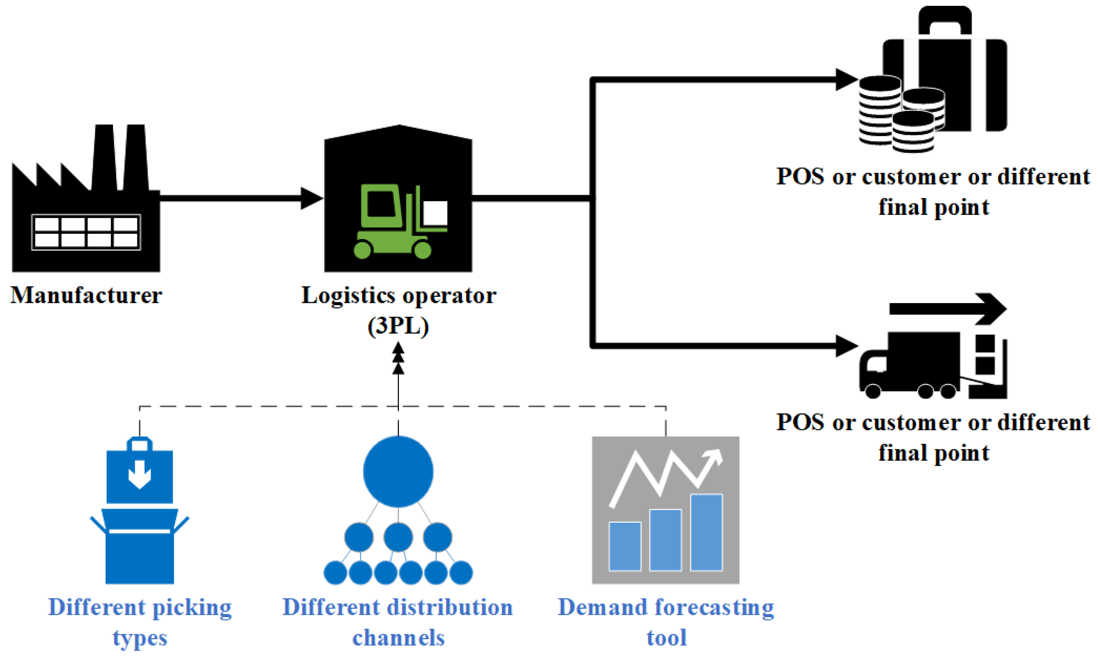
Figure 2.
Hypotheses verified in the paper.
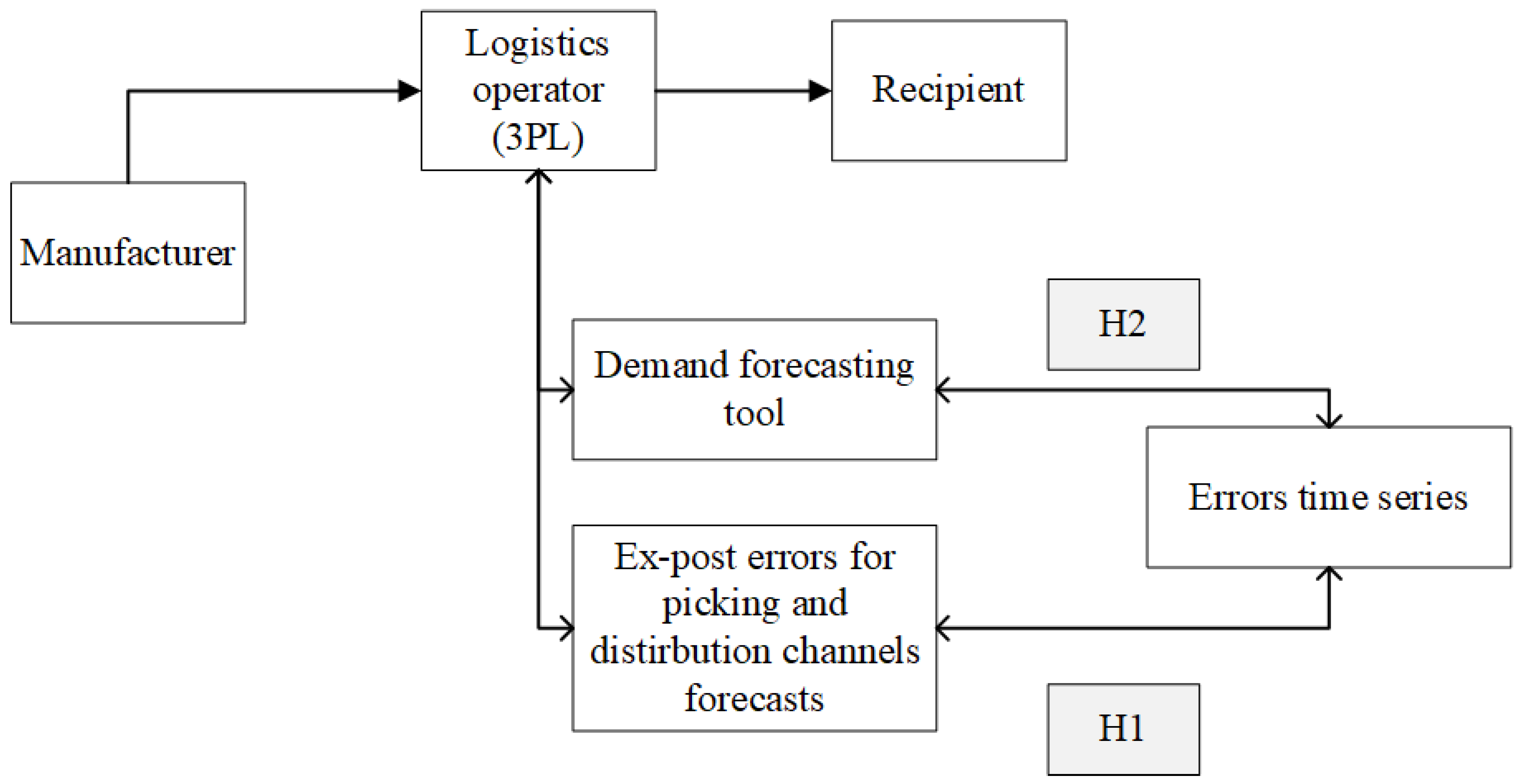
Figure 3.
Time series of forecasting errors for the considered channels.
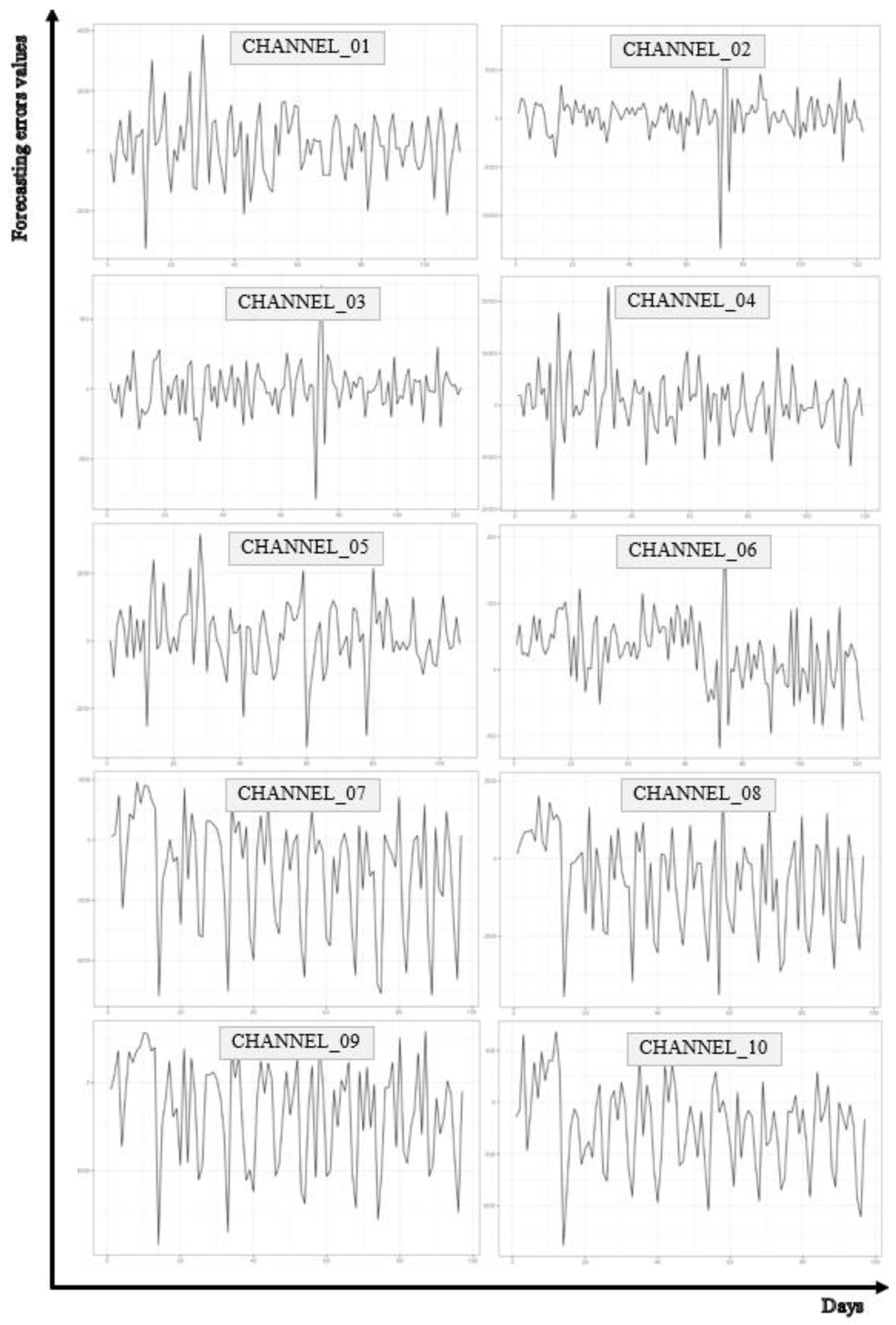
Figure 4.
The STL decomposition of channel_03 errors time series.
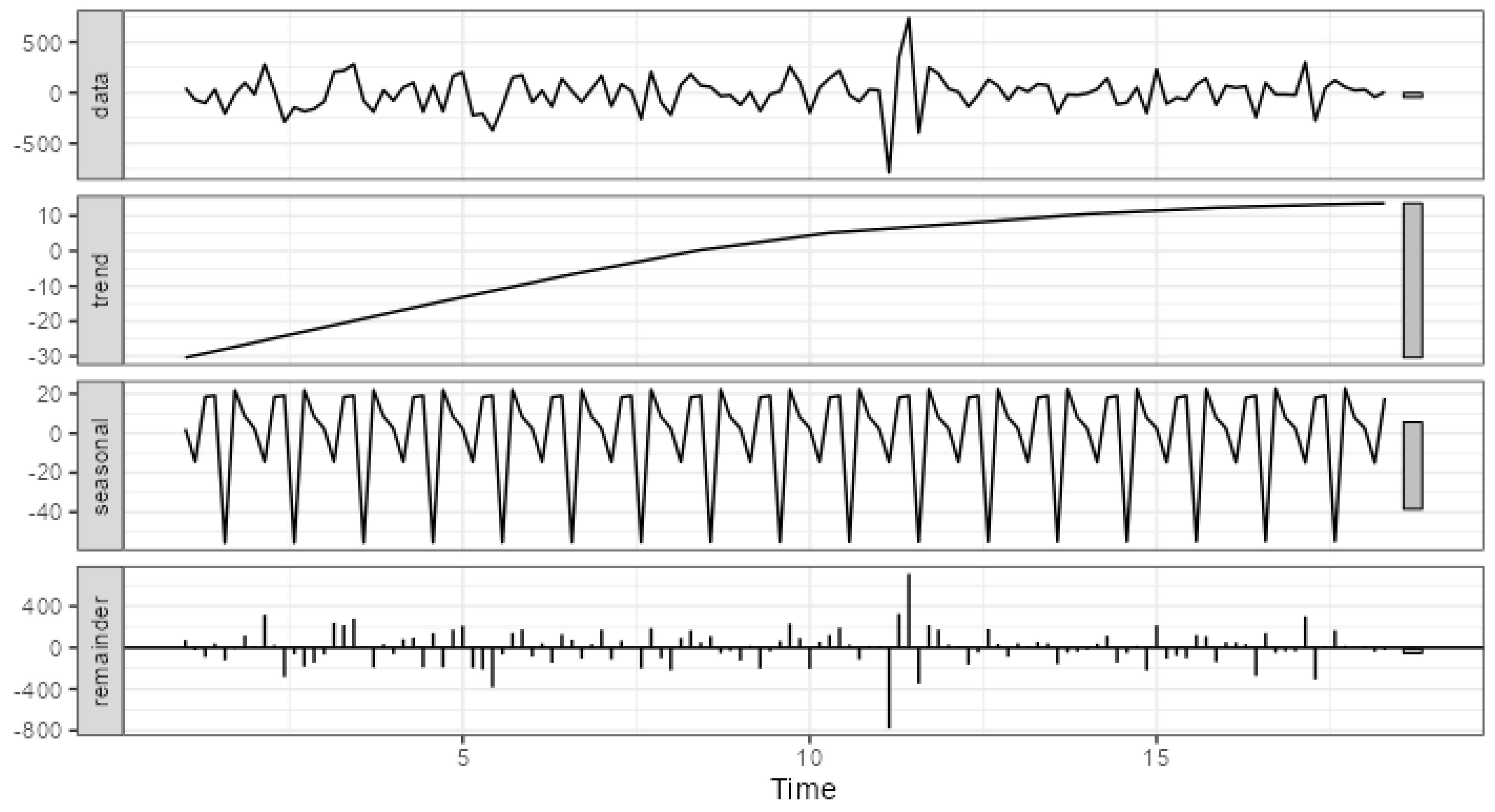
Figure 5.
The STL decomposition of channel_10 errors time series.
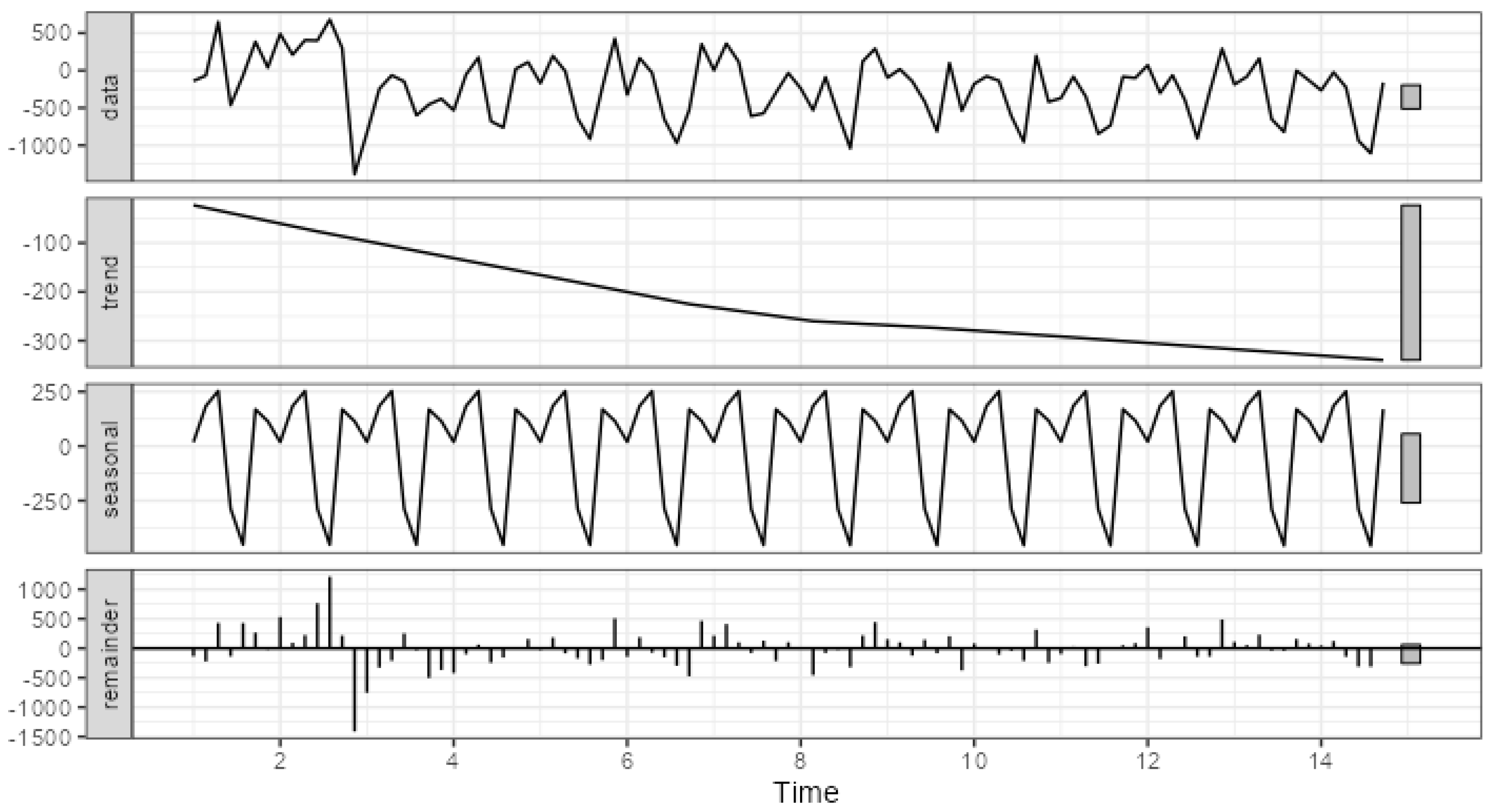

Table 1.
Examples of the new functionalities of the model used by the logistic operator when compared to the traditional ARIMA model.
Table 1.
Examples of the new functionalities of the model used by the logistic operator when compared to the traditional ARIMA model.
| New functionality | New functionality general outline |
|---|---|
| Automatic detection of seasons | The model detects seasons automatically and uses them to adapt the forecasting algorithm accordingly. |
| Outlier detection | The model detects outliers automatically to identify and delete outliers from data before the model is adapted. This helps to improve the model accuracy by reducing the effect of extreme values in the data. |
| Handling of missing values | The model may handle missing values in the data by completing them using the linear interpolation method. Thanks to that, the model uses as much data as possible which may improve forecast accuracy. |
| Nonlinear transformation | The model offers the ability to use nonlinear transformations for data, including logarithmic or exponential transformations. This may help to capture more complex data patterns which are not represented by the linear ARIMA model. |
Table 2.
General data characteristics for the analyzed distribution networks.
| Manufacturer | Distribution channel | Picking method for which the release volumes were forecast | Designation of the channel and the picking method in the paper | General data characteristics |
|---|---|---|---|---|
| 1 | Hospitals | Picking of individual units | Channel_01 | 182 days of daily forecast history |
| Picking of cardboard boxes | Channel_02 | |||
| Picking of shrink-wrap packagings | Channel_03 | |||
| Wholesalers | Picking of individual units | Channel_04 | ||
| Picking of cardboard boxes | Channel_05 | |||
| Picking of shrink-wrap packagings | Channel_06 | |||
| 2 | e-commerce | Picking of individual units from the mezzanine | Channel_07 | 96 days of daily forecast history |
| Picking of individual units from the racks | Channel_08 | |||
| Picking of cardboard boxes | Channel_09 | |||
| Retail stores | Picking of cardboard boxes | Channel_10 |
Table 3.
Main methods and functionalities of R employed in the forecasting error analysis.
| Functionality | Functionalities used |
|---|---|
| Analysis of the forecasting error randomness | bartels.rank.test(),runs.test(),cox.stuart.test(),difference.sign.test() |
| Stationarity analysis | adf.test() (Trapletti, Hornik, 2023) |
| Autocorrelation analysis | acf(), Box.test() |
| STL decomposition of time series | stl(t.window = length(number_of_errors), s.window = length(number_of_errors)) |
| Trend presence analysis | notrend_test(tests = “t”),notrend_test(tests = “MK”), notrend_test(tests = “WAVK”) (Lyubchich V. et al. 2023) |
| Seasonality component presence analysis | combined_test(), qs(), fried(), kw.p(), seasdum(), welch() (Olech, 2021) |
Table 4.
The basic parameters of the forecasting error distribution for the analyzed channels.
| Channel_01 | Channel_02 | Channel_03 | Channel_04 | Channel_05 | Channel_06 | Channel_07 | Channel_08 | Channel_09 | Channel_10 | |
|---|---|---|---|---|---|---|---|---|---|---|
| Mean | 176 | 245 | 0 | 574 | 126 | 25 | -1387 | -706 | -1583 | -228 |
| Std.Dev | 1095 | 2268 | 174 | 5665 | 1017 | 52 | 2822 | 1602 | 2969 | 420 |
| Min | -3249 | -13376 | -786 | -18267 | -3160 | -118 | -7773 | -4455 | -9193 | -1388 |
| Q1 | -581 | -752 | -97 | -2221 | -416 | -3 | -2806 | -1981 | -4357 | -532 |
| Median | 172 | 507 | 15.5 | 297 | 149 | 29.5 | -687 | -175 | -732 | -147 |
| Q3 | 916 | 1419 | 84 | 3571 | 765 | 57 | 629 | 545 | 863 | 21 |
| Max | 3868 | 8508 | 740 | 22774 | 3151 | 202 | 2901 | 2436 | 2918 | 681 |
| MAD | 1103 | 1559 | 145 | 4340 | 859 | 45 | 2423 | 1634 | 2950 | 397 |
| IQR | 1476 | 2117 | 179.5 | 5653 | 1171.25 | 59 | 3435 | 2526 | 5220 | 553 |
| CV | 6.212 | 9.272 | - | 9.876 | 8.040 | 2.079 | -2.034 | -2.268 | -1.875 | -1.843 |
| Skewness | 0.037 | -1.606 | -0.201 | 0.279 | -0.278 | -0.161 | -0.715 | -0.354 | -0.531 | -0.288 |
| SE.Skewness | 0.229 | 0.219 | 0.219 | 0.222 | 0.235 | 0.219 | 0.245 | 0.245 | 0.245 | 0.245 |
| Kurtosis | 0.954 | 11.280 | 4.387 | 2.270 | 1.330 | 0.567 | -0.487 | -0.774 | -0.726 | -0.354 |
| N.Valid | 111 | 122 | 122 | 119 | 106 | 122 | 97 | 97 | 97 | 97 |
Table 5.
Randomness (alternative hypothesis: nonrandomness).
| Channel | bartels.rank.test | runs.test | cox.stuart.test | difference.sign.test |
|---|---|---|---|---|
| Channel_01 | 0.887 | 0.716 | 0.798 | 0.274 |
| Channel_02 | 0.037* | 0.029* | <0.001* | 0.274 |
| Channel_03 | 0.545 | 0.716 | 0.443 | 0.530 |
| Channel_04 | 0.964 | 0.064 | 0.435 | 0.343 |
| Channel_05 | 0.227 | 0.172 | 0.583 | 0.402 |
| Channel_06 | 0.270 | 0.338 | >0.999 | 0.513 |
| Channel_07 | 0.026* | 0.412 | 0.312 | <0.001* |
| Channel_08 | 0.664 | 1.000 | 0.059 | 0.080 |
| Channel_09 | 0.117 | 0.218 | 0.006* | 0.162 |
| Channel_10 | 0.009* | 0.305 | 0.029* | 0.726 |
Table 6.
ACF coefficient values with their critical significance and p-values for Ljung-Box test. The values refer to the first seven delays.
Table 6.
ACF coefficient values with their critical significance and p-values for Ljung-Box test. The values refer to the first seven delays.
| Channel | ACF (coefficient) | ACF (p-value) | Ljung-Box test (p-value) |
|---|---|---|---|
| Channel_01 | -0.175, -0.235, 0.153, -0.080, 0.054, -0.166, 0.057 |
0.053, 0.01, 0.091, 0.376, 0.548, 0.067, 0.529 | 0.050, 0.005, 0.003, 0.006, 0.011, 0.005, 0.008 |
| Channel_02 | 0.088, 0.118, 0.21, 0.139, 0.235, 0.086, 0.157 | 0.33, 0.193, 0.021, 0.126, 0.009, 0.341, 0.083 | 0.324, 0.256, 0.04, 0.029, 0.003, 0.004, 0.002 |
| Channel_03 | -0.109, -0.243, 0.096, -0.155, -0.097, 0.019, -0.026 |
0.229, 0.007, 0.287, 0.087, 0.286, 0.83, 0.776 | 0.223, 0.012, 0.018, 0.01, 0.013, 0.025, 0.043 |
| Channel_04 | -0.001, -0.257, -0.006, -0.009, 0.126, 0.047, 0.013 | 0.988, 0.005, 0.945, 0.921, 0.168, 0.607, 0.89 | 0.988, 0.017, 0.044, 0.087, 0.071, 0.108, 0.165 |
| Channel_05 | 0.087, -0.201, -0.011, 0.051, 0.059, -0.069, -0.143 | 0.369, 0.039, 0.909, 0.602, 0.545, 0.474, 0.141 | 0.362, 0.072, 0.153, 0.234, 0.311, 0.369, 0.262 |
| Channel_06 | 0.099, -0.314, -0.116, 0.109, 0.05, -0.107, -0.004 | 0.297, 0.001, 0.223, 0.253, 0.599, 0.261, 0.967 | 0.29, 0.002, 0.003, 0.004, 0.008, 0.009, 0.017 |
| Channel_07 | 0.273, -0.009, -0.147, -0.128, -0.062, 0.131, 0.4 | 0.007, 0.932, 0.147, 0.208, 0.538, 0.197, 0, 0.11 | 0.006, 0.024, 0.021, 0.022, 0.038, 0.034, <0.001 |
| Channel_08 | 0.011, 0.023, -0.01, -0.066, -0.084, 0.203, 0.375 | 0.914, 0.821, 0.921, 0.514, 0.407, 0.045, 0, 0.321 | 0.912, 0.968, 0.995, 0.971, 0.938, 0.466, 0.004 |
| Channel_09 | 0.132, -0.055, 0.037, 0.07, 0.219, 0.071, 0.245 | 0.193, 0.587, 0.715, 0.488, 0.031, 0.487, 0.016 | 0.187, 0.358, 0.533, 0.608, 0.173, 0.221, 0.041 |
| Channel_10 | 0.275, -0.155, -0.041, -0.086, -0.107, 0.131, 0.444 | 0.007, 0.126, 0.684, 0.395, 0.292, 0.197, 0, 0.766 | 0.006, 0.007, 0.017, 0.027, 0.033, 0.031 |
Table 7.
The results of the analysis of the forecasting error series relating to STL decomposition.
| Channel | Trend_stl | Season_stl | MAE_error | MAPE_error | Remainder_MAE_stl | Quotient_stl |
|---|---|---|---|---|---|---|
| Channel_03 | 0.007 | 0.021 | 125 | 0.593 | 124 | 0.994 |
| Channel_02 | 0.158 | 0.030 | 46 | 0.608 | 36 | 0.775 |
| Channel_06 | 0.006 | 0.037 | 861 | 29.518 | 816 | 0.947 |
| Channel_01 | 0.000 | 0.045 | 1500 | 0.425 | 1433 | 0.955 |
| Channel_04 | 0.029 | 0.049 | 4129 | 5.095 | 4009 | 0.971 |
| Channel_05 | 0.010 | 0.053 | 768 | 16.901 | 735 | 0.957 |
| Channel_09 | 0.145 | 0.128 | 109 | 0.455 | 90 | 0.828 |
| Channel_07 | 0.099 | 0.230 | 1010 | 0.341 | 779 | 0.771 |
| Channel_08 | 0.130 | 0.276 | 1363 | 0.279 | 984 | 0.722 |
| Channel_10 | 0.092 | 0.380 | 366 | 0.268 | 226 | 0.617 |
Table 8.
p-value in tests for the Null Hypothesis of no Trend.
| Channel | Student’s t-test (linear trend) | Mann–Kendall Test (monotonic trend) | WAVK test (possibly non-monotonic trend) |
|---|---|---|---|
| Channel_01 | 0.927 | 0.690 | 0.052 |
| Channel_02 | <0.001* | <0.001* | <0.001* |
| Channel_03 | 0.426 | 0.415 | 0.041* |
| Channel_04 | 0.042* | 0.067 | 0.498 |
| Channel_05 | 0.357 | 0.340 | 0.578 |
| Channel_06 | 0.396 | 0.524 | 0.257 |
| Channel_07 | 0.023* | 0.025* | 0.071 |
| Channel_08 | 0.006* | 0.001* | 0.729 |
| Channel_09 | <0.001* | <0.001* | 0.020* |
| Channel_10 | 0.119 | 0.090 | 0.600 |
Table 9.
p-value in tests for the Null Hypothesis of no seasonality.
| Channel | combined.kwr | qs.p | fried.p | kw.p | seasdum.p | welch.p |
|---|---|---|---|---|---|---|
| Channel_01 | 0.293 | >0.999 | 0.098 | 0.106 | 0.504 | 0.179 |
| Channel_02 | 0.422 | >0.999 | 0.905 | 0.729 | 0.760 | 0.723 |
| Channel_03 | 0.943 | >0.999 | 0.976 | 0.969 | 0.874 | 0.829 |
| Channel_04 | 0.649 | >0.999 | 0.848 | 0.546 | 0.466 | 0.368 |
| Channel_05 | 0.570 | >0.999 | 0.187 | 0.307 | 0.500 | 0.173 |
| Channel_06 | 0.672 | >0.999 | 0.638 | 0.553 | 0.684 | 0.629 |
| Channel_07 | < 0.001 | < 0.001 | < 0.001 | < 0.001 | 0.001 | < 0.001 |
| Channel_08 | < 0.001 | 0.026 | 0.003 | 0.001 | < 0.001 | < 0.001 |
| Channel_09 | 0.052 | >0.999 | 0.058 | 0.013 | 0.055 | 0.025 |
| Channel_10 | < 0.001 | < 0.001 | < 0.001 | < 0.001 | < 0.001 | < 0.001 |
Disclaimer/Publisher’s Note: The statements, opinions and data contained in all publications are solely those of the individual author(s) and contributor(s) and not of MDPI and/or the editor(s). MDPI and/or the editor(s) disclaim responsibility for any injury to people or property resulting from any ideas, methods, instructions or products referred to in the content. |
© 2024 by the authors. Licensee MDPI, Basel, Switzerland. This article is an open access article distributed under the terms and conditions of the Creative Commons Attribution (CC BY) license (http://creativecommons.org/licenses/by/4.0/).
Copyright: This open access article is published under a Creative Commons CC BY 4.0 license, which permit the free download, distribution, and reuse, provided that the author and preprint are cited in any reuse.


