
Submitted:
11 September 2024
Posted:
11 September 2024
Read the latest preprint version here
Abstract
Modular inversion on large operands is a time-consuming calculation used in elliptic curve cryptography. Its hardware implementation requires extensive hardware resources such as lookup tables and registers. We investigate state-of-the-art modular inversion algorithms and evaluate the performance and cost of the algorithms and their hardware implementations. We then propose a high-radix modular inversion algorithm aimed at short execution time and low hardware cost. We present a detailed radix-8 hardware implementation based on 256-bit primes in Verilog HDL and compare its cost performance with other implementations. Our implementation on the Altera Cyclone V FPGA chip uses 1227 ALMs (Adaptive logic modules) and 1037 registers. The modular inversion calculation takes 3.67 microseconds. The AT (Area time) factor is 8.30, outperforming other implementations. We also present an implementation of elliptic curve cryptography using the proposed radix-8 modular inversion algorithm. The implementation results also show that our modular inversion algorithm is more efficient in area time than other algorithms.
Keywords:
computer security
; elliptic curve cryptography
; modular inversion
; hardware
; Verilog HDL
; FPGA
; cost performance evaluation
1. Introduction
Modular inversion is an important computation in elliptic curve cryptography (ECC). ECC provides a secure key agreement between two parties over an insecure network. It calculates points on an elliptic curve over a finite field (such as a field of prime numbers) based on point addition (PA) and point doubling (PD) computations. In affine coordinates, PA and PD must calculate the slope of a line. Such calculations involve costly modular inversions. In projective or Jacobian coordinates, PA and PD do not require such calculations, but a modular inversion is still required to transform the points to affine coordinates to obtain the same key for the two parties.
Given a prime number m, the inverse r of a number a with is defined as . There are mainly two popular methods for calculating modular inversion:
- Extended Euclidean Algorithm (EEA) without using divisions.
- Using Fermat’s Little Theorem [1]: .
We will see that the method using Fermat’s Little Theorem takes longer time and requires more registers than EEA. Therefore, we will focus our design on using the EEA.
The EEA inherently needs divisions. It calculates the largest integer quotient and calculates the remainder based on the quotient. The divisions can be replaced by addition, subtraction, and shift operations. For simplicity, we will also refer to EEA which does not use divisions as EEA.
For calculating , EEA first initializes with , respectively. Then EEA repeats calculations containing only addition, subtraction, and shift operations on until or . Finally, the modular inversion result is available by adjusting x or y, corresponding to or . A modular inversion algorithm is said to be fast if u or v reaches 1 quickly.
The widely used modular inversion algorithm is Algorithm 2.22, proposed by Hankerson, Menezes, and Vanstone [2]. It repeatedly shifts u or v to the right when u or v is even. Correspondingly, x is also shifted to the right with the shift of u; y is also shifted to the right with the shift of v. Note that when x or y is odd, m will be added before shift. This ensures that the value being right-shifted is even since the prime number m is odd. Next, if , u and x will be replaced by and , respectively. Otherwise, v and y will be replaced by and , respectively. Finally, the result is if and otherwise. Hossain and Kong [3] revised Algorithm 2.22 by adding m to x or y if it is negative. This ensures that x and y are non-negative. Daly, Marnane, Kerins, and Popovici [4] revised Algorithm 2.22 by dividing or by two because the subtraction result is even (both u and v are odd before the subtraction). Correspondingly, or needs also to be divided by two: If or is odd, m is added before the division. Division by two is done by shifting one bit to the right. Mrabet, El-Mrabet, Bouallegue, Mesnager, and Machhout proposed a modular inversion algorithm [5] with . Instead of or , as Algorithm 2.22 does, they perform for new u or v. This operation slows down the speed at which u or v reaches 1, increasing execution time. Chen and Qin proposed a modular inversion algorithm [6] that uses only adders. Subtractions are performed by addition with inversion and addition by 1. Choi, Lee, Kong, and Kim proposed a modular inversion algorithm [7] that replaces the repeated shift of u or v and the corresponding shift of x or y in Algorithm 2.22 by a selection of or , or a selection of or , based on the even/odd of v or u. This simplifies the circuit by replacing adders with multiplexers, reducing the circuit delay. Also, they use and , instead of v and y, during the calculation. This merges and into and merges and into , reducing the circuit cost. Mixed radix-4 modular inversion algorithms are investigated in [7,8,9,10]. If u or v is divisible by four, u or v is shifted to the right by two bits. Otherwise, if u or v is even (divisible by two), u or v is shifted to the right by one bit. Otherwise (both u and v are odd), or is shifted to the right by one bit and assigned to u or v. Correspondingly, x or y is adjusted by adding , m, or and shifted to the right by two bits or one bit. [8] proposed a radix-4 modular inversion algorithm that uses a sequential condition checking for the calculations of u, v, x, and y. [9] implemented the SM2 ECC protocol. The iterations of the modular inversion are controlled by the bit counter , resulting in unnecessary iterations. Using u and v to control the iterations will finish the calculation quickly. [10] gave a radix-4 version of Algorithm 2.22. Dong, Zhang, and Gao proposed a mixed radix-8 modular inversion algorithm [11] that uses extensive hardware resources.
The AT (Area time) factor is often used for comparisons between implementations. It is defined as the execution time in milliseconds multiplied by the required hardware resources consisting of registers and lookup tables or ALMs (Adaptive logic modules).
In this paper, we implement and evaluate all the algorithms mentioned above. We then propose a mixed radix-8 modular inversion algorithm aimed at short execution time and small hardware resources. We give its detailed hardware implementation in Verilog HDL based on 256-bit primes. It has lower hardware costs for ALMs and registers and has better performance than other algorithms. The implementation on the Altera Cyclone V FPGA chip uses 1227 ALMs and 1037 registers and takes 3.67 microseconds for the modular inversion computation. It achieves an AT factor of 8.30, lower than all other implementations. We also implement ECC using different modular inversion algorithms and compare their cost performance.
The rest of the paper is organized as follows. Section 2 introduces ECC and modular inversion algorithms. Instead of pseudocodes, all modular inversion algorithms are provided in Python code. Section 3 proposes a mixed radix-8 modular inversion algorithm, gives its hardware implementation in Verilog HDL, and compares its cost performance with other algorithms. Section 4 provides an ECC implementation using the proposed algorithm and compares its cost performance with the ECC implementations using other modular inversion algorithms. And Section 5 concludes the paper.
2. ECC and Modular Inversion Algorithms
This section briefly introduces elliptic curve cryptography and modular inversion algorithms based on the extended Euclidean algorithm.
2.1. Elliptic Curve Cryptography
ECC [12,13] relies on the fact that scalar point multiplication can be computed, but it is almost impossible to compute d given only the original point P and the point of the product Q. An ECC over the finite field of an n-bit prime number m can use the equation:
For example, Secp256k1 [14] elliptic curve used in Ethereum Blockchain uses a 256-bit . Secp256k1 defines and gives a point on the elliptic curve as follows.
a = 0x0000000000000000000000000000000000000000000000000000000000000000
b = 0x0000000000000000000000000000000000000000000000000000000000000007
m = 0xfffffffffffffffffffffffffffffffffffffffffffffffffffffffefffffc2f
x = 0x79be667ef9dcbbac55a06295ce870b07029bfcdb2dce28d959f2815b16f81798
y = 0x483ada7726a3c4655da4fbfc0e1108a8fd17b448a68554199c47d08ffb10d4b8
The elliptic curve Diffie–Hellman (ECDH) key exchange protocol can be used by two parties, Alice and Bob for example, to establish a shared secret key over an insecure network [14,15]. The ECDH protocol is shown in Table 1.
Because , , and , we have . Below is an ECDH key exchange example using Secp256k1. We can see that the two parties, Alice and Bob, have the same shared secret key (Qabx = Qbax).
- Alice keeps secret and exposes :
da = 0x0e26233af432c34fa2523e72b64ebcf5abb4f7cb07d8f25909160a50f584f461
Qax = 0x672751a7b8ec03f4610c364d3776fc5200f401aa26074b10d33c2c202fc63330
Qay = 0xdbf4a0758d81414d2ee049a07c3d8288428235dec9dbfb7fb15d6f478cb4ccf6
- Bob keeps secret and exposes :
db = 0xbbb481621f91b8e9225649109919a7962cec4225c981b6b68b4f8d8a356cc6d9
Qbx = 0x09aff71612598a88d5299ae81e3161a2c9045f343315da8cfabb4dc55253041f
Qby = 0x736b118369583448c0b77eed11ac26af31450d406130d82a1bc56cc3a1835b1d
- Alice obtains and calculates :
Qabx = 0x0f675b3195fd6a6f06c9a6960ff2a4f647f637f513c8bb7bedc8a89311f62df2
Qaby = 0x79de922da4db277fe0c674277243c1dfd0653913d037fb07e955c3cdf21e69c7
- Bob obtains and calculates :
Qbax = 0x0f675b3195fd6a6f06c9a6960ff2a4f647f637f513c8bb7bedc8a89311f62df2
Qbay = 0x79de922da4db277fe0c674277243c1dfd0653913d037fb07e955c3cdf21e69c7
- Now, Alice and Bob have the same secret key (Qabx = Qbax). They can use symmetric-key cryptography for subsequent communications. A third party, Eve for example, knows , P, , and , but cannot calculate the same secret key.
2.2. Point Addition and Point Doubling
Scalar point multiplication calls point addition (PA) and point doubling (PD).
2.2.1. Point Addition
Given and , the formulas for point addition on elliptic curve are shown as follows, where is the slope of the line through points P and Q.
The point at infinity, denoted , is included in the group of elliptic curves and is defined as for . By this definition, . In our implementation, is represented as . In the case of , . In the case of , . We give the point addition algorithm over the finite field of in Algorithm 1. In the case of , (line 5 in the algorithm). In the case of , , we perform the point doubling (line 6 in the algorithm).
| Algorithm 1 PA (P, Q, m, a) (Point Addition in Affine Coordinates). |
|
inputs: Points and ; m and a in
output:
begin
1 , , , ,
2 if return Q /* */
3 if return P /* */
4 if
5 if return /* */
6 else return PD (P, m, a) /* */
7
8
9
10 return /* */
end
|
An example of point addition on the Secp256k1 curve is shown below where , , and in affine coordinates.
Px = 0xfc7dafb820a20da1a73c36465f2fe37bfd98ce4ef3a10a5df110abda03b20a3d
Py = 0xa442a2d1b8bde4a09e45725add5daae89e726b56f0e8fe6609dacaf5279b2564
Qx = 0xe106c069450b2663febb83e29b67fa93c4c48a45d5fbe7ce4ddb8ceb601fcc1d
Qy = 0xc9da9bd440909c8862c06a44d432d2dd45284636b7049b9bf4695f9e4018d2f2
Rx = 0xfd52a0334e16f8cf45a6b0820887a9e8b1b180516a76c8adfef95df98aeef376
Ry = 0xb0fe3f04cc4c64fd66a133b8c97b4905771238f8ba89631efb85a8059e969a49
2.2.2. Point Doubling
Given , the formulas for point doubling on elliptic curve are shown as follows, where is the slope of the tangent line of the elliptic curve at point P.
We give the point doubling algorithm over the finite field of in Algorithm 2. In the case of (vertical tangent line), (line 2 in the algorithm).
| Algorithm 2 PD (P, m, a) (Point Doubling in Affine Coordinates). |
|
inputs: Point ; m and a in
output:
begin
1 , ,
2 if return /* vertical tangent */
3
4
5
6 return /* */
end
|
An example of point doubling on the Secp256k1 curve is shown below where and in affine coordinates.
Px = 0x6034b56424fb31ea6ec5483b52ae5d07d6f3ef80264d769ae2714abb83fb279a
Py = 0xfe4cde1ff7546a87f906f50ab1002fda7811828ea6fc467a44d1c6c11aa65a37
Rx = 0x5491ee8b73a4ed9713ed32e467de5100b80861babf8ffd09fd595ab457d042c9
Ry = 0xf91e6a4e132a1bdf4f5c846559431ec7373de8872b719f188b5902932f0a2b30
The computation of in PA and PD requires modular division, which can be realized by a modular inversion algorithm based on the extended Euclidean algorithm.
2.3. Modular Inversion Algorithms
Given a prime number m, the inverse r of a number a with is defined as
That is, . The Python code below implements the modular inversion calculation using Fermat’s Little Theorem. When executed, it outputs 4 4 4. The first output value is calculated by the code, and the rest are for checking. This calculation consists of costly modular multiply and modular squaring, very similar to RSA exponentiation [16].


The extended Euclidean algorithm can be used for the modular inversion calculation. Below is the fundamental extended Euclidean algorithm given in Python code (modinv_algo_1.py), where q is the integer quotient of u divided by v.
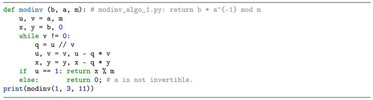
Considering . u and x are initialized with a and 1, respectively. At each iteration, u and x are modified with similar calculations. Therefore, when u reaches 1 from a, x reaches the reciprocal of a from 1. If m is a prime number, the greatest common divisor of a and m is guaranteed to be 1, and we can always get the inverse result of a. With the initialization of x with b, the algorithm performs the modular division .
An example of running modinv_algo_1.py using modinv(1, 3, 11) is shown in Table 2 (, , and ). The calculation finishes when . Because , the result . We can check the correctness as follows: .
The algorithm requires division, which is expensive. We can remove division by setting the quotient to 0 or 1, as shown below (modinv_algo_2.py).


The algorithm yields a quotient of 0 or 1 based on the comparison of u and v. If the quotient is a 1, a subtraction is performed. Otherwise, no calculation is performed, resulting in a slow calculation speed. The calculation of modinv (1, 3, 11) will require 9 iterations. We can modify the algorithm as follows (modinv_algo_3.py). This reduces the number of iterations by about half.
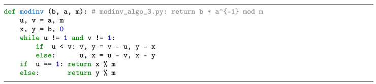
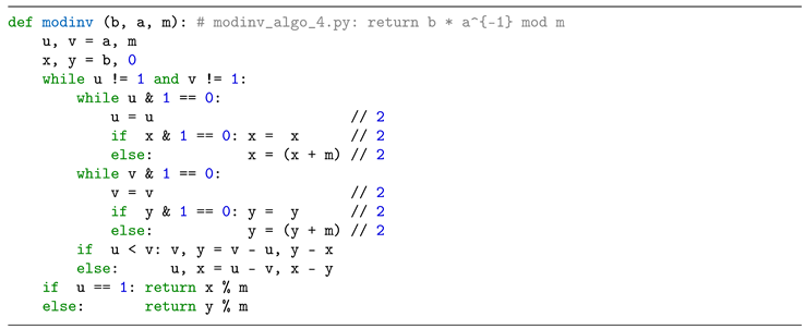
We can check u first before the subtractions. If it is even, we can shift it to the right by one bit (the least significant bit 0 is shifted out). Correspondingly, x must also be shifted. To ensure the shifted value is even, m will be added to x before the shift if x is odd. Note that m is odd because it is a prime number. This shift of u and x can be performed repeatedly until u becomes an odd number. Similar actions can be applied to v and y. Then we can have an algorithm as follows (modinv_algo_4.py). In fact, this is Algorithm 2.22 provided in [2] and implemented in Verilog HDL in [17].
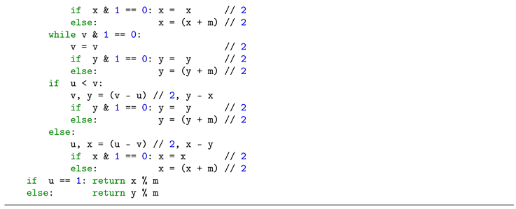
When the two inner while loops finish, u and v are both odd numbers. Therefore or is even. Then we can shift it to the right by one bit. Correspondingly, or must also be shifted. If or is odd, m must be added before the shift so that the bit being shifted out is 0. The algorithm is shown below (modinv_algo_5.py).

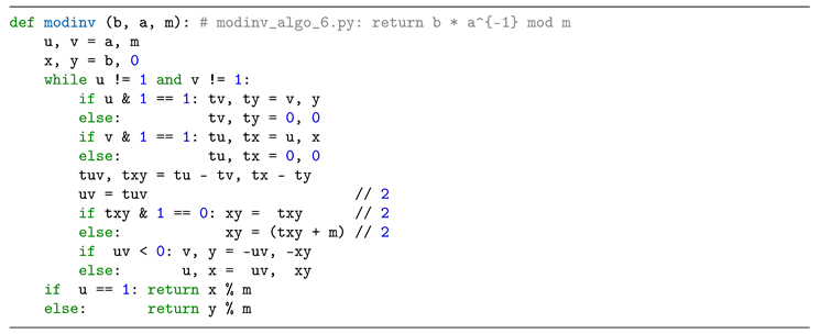
The two inner while loops can be replaced by assigning u, x, v, y, or 0 to the temporary variables , , , and . The following assignments make even, so we can shift it to the right by one bit: (1) If both u and v are odd, those temporary variables are assigned with u, x, v, y, respectively. (2) If u is even and v is odd, those temporary variables are assigned with u, x, 0, 0, respectively. (3) If u is odd and v is even, those temporary variables are assigned with 0, 0, v, y, respectively. Such elimination shortens the latency from the carry propagation adder to the multiplexer and speeds up the calculation. The algorithm is shown below (modinv_algo_6.py).
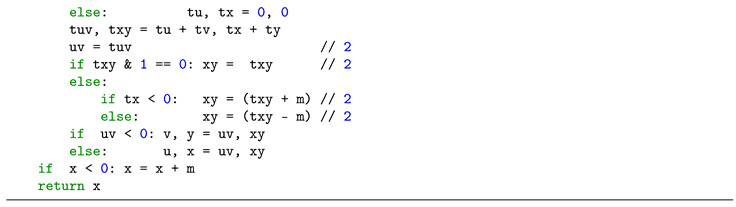
The algorithm above requires calculations of , , , and . We can unify these calculations with negative assignments and to v and y, respectively. That is, becomes , and becomes with the negative assignments to v and y. Similarly, becomes , and becomes with the negative assignments to v and y. Therefore, and are sufficient for the calculation. The algorithm is given below (modinv_algo_7.py). Because of the negative assignments to v and y, v is initialized with and y is initialized with . Note that x is never greater than or equal to m. Therefore, no adjustment of or is required.

A modular inversion algorithm is said to be good when u reaches 1 quickly (high performance) and the algorithm uses a small number of adders and subtractors (low cost).
3. Proposed Radix-8 Modular Inversion Algorithm and its Performance
The proposed mixed radix-8 modular inversion algorithm is shown below (modinv_radix_8.py). To calculate , we initialize and with the negative assignment to v and y. The temporary variable is assigned with u or 0 and the temporary variable is assigned with v or 0 so that is even. If the three least significant bits of are 000, it is shifted to the right by three bits (radix-8). Otherwise, if the two least significant bits of are 00, it is shifted to the right by two bits (radix-4). Otherwise, it is shifted to the right by one bit (radix-2), because is even.
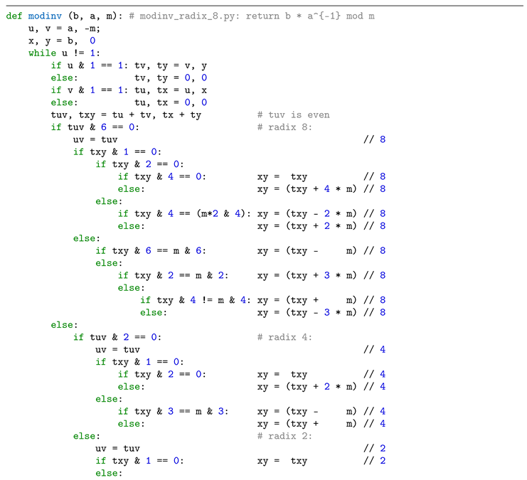

Correspondingly, and are arranged and is also shifted to the right by three bits, two bits, or one bit. The bits being shifted out must be 0. Therefore, we need to adjust using the prime number m before shifting. Table 3 lists such adjustments based on the three least significant bits of and the three least significant bits of m for the radix-8 operations, where x represents a don’t care. The three least significant bits of the adjusted value are 000, as shown in the comment column of the table.
Similarly, Table 4 lists the adjustments based on the two least significant bits of and the two least significant bits of m for the radix-4 operations. The two least significant bits of the adjusted value are 00, as shown in the comment column of the table.
An example of is shown below. The modinv_radix_8 algorithm takes 206 iterations to reach and . In contrast, the modinv_radix_4 and modinv_radix_2 algorithms require 243 and 356 iterations, respectively.
b = 0x9cfa1c993911914be0f15bd74a878abe0079c6254b961b82e1abda76387d1d85
a = 0xd5076ae274e874c2eb0f7778717c39460236549ddd9fc651e68a0c0e787b4ce8
m = 0xfffffffffffffffffffffffffffffffffffffffffffffffffffffffefffffc2f
c = 0xe8e5ac2e1d3358894ce1b3342737b38c39b89059dd55d3c4741626de8270228e
To reduce the number of adders, we use multiplexers to select an appropriate value and assign it to the temporary variable . And then we perform . Based on the three least significant bits of , we assign , , or (shift right) to . Figure 1 shows the block diagram of the proposed mixed radix-8 modular inversion circuit. Because we perform addition for , and are replaced by and , respectively. Also, for the addition, we prepare that can be obtained by inverting all the bits of m and setting the right-most bit to 1 because m is odd. The registers u, v, x, and y are shown with red rectangles. The multiplexers are drawn with green rectangles. The blue rectangles are adders. The Verilog HDL implementation uses continuous assignment to compute and and writes them to the corresponding registers on the rising edge of the clock signal. Note that we have to use adders for generating , , and , which are not shown in the figure.
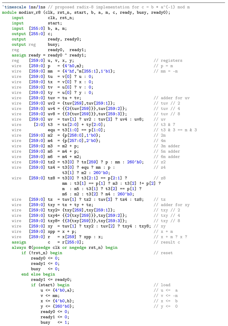
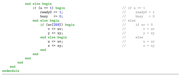
Below we give the hardware implementation code in Verilog HDL for the proposed mixed radix-8 modular inversion algorithm (modinv_r8.v). The signals start and ready indicate the start of the modular inversion calculation and the availability of the calculation result, respectively. Because we use Secp256k1 elliptic curve, the input and output signals b, a, m, and c are 256 bits. During the calculations, we use 260 bits for the internal signals.
Below is the testbench Verilog HDL code used to simulate modinv_r8.v.
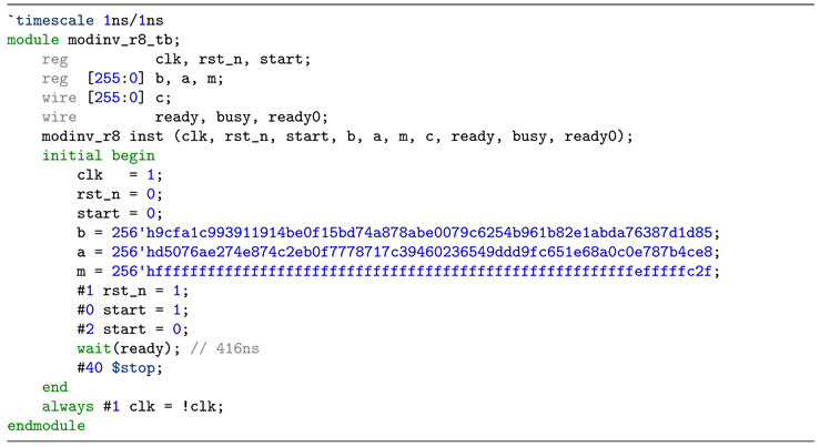
Figure 2 shows the functional simulation waveform, generated with ModelSim. The result c is available at 416ns. That is, the calculation takes 208 clock cycles.
We have implemented the modular inversion algorithms on the Altera Cyclone V 5CGXFC9E7F35C8 FPGA chip. Table 5 lists the cost performance of the modular inversion algorithms. The column of Cycles shows the required number of clock cycles when executing the modular inversion algorithm. The column of Freq.(MHz) shows the clock frequency in MHz at which the circuit can work. The column of Latency(s) shows the execution time in microseconds calculated by dividing the clock cycles by the clock frequency. The column of ALMs shows the required number of adaptive logic modules. The column of Registers shows the required number of flip-flops. The flip-flops are mainly used to store u, v, x, and y. Their contents are updated on every clock cycle. The last column shows the AT factor, which is the product of the Latency in milliseconds and the sum of ALMs and Registers.
The row of [1] in the table shows the performance and cost of modular inversion using Fermat’s Little Theorem . It consists of costly modular multiply and modular squaring, very similar to RSA exponentiation [16]. Its AT factor is much higher than others. The remaining rows show the performance and cost of the EEA-based modular inversion algorithms. The number of registers used by [2,3,8], and [10] is larger than others. This is because extra registers are used to adjust the value of x or y so that the modular inversion result is within the range of 0 and m. Our algorithm implementation achieves an execution time of 3.67s and an AT factor of 8.30, outperforming all other implementations. Figure 3 shows an intuitive view of latency and AT histograms.
4. ECC Implementation with Proposed Modular Inversion Algorithm
ECC relies on scalar point multiplication. Suppose is a point on the curve, the scalar point multiplication gets the that is also on the curve, where is an n-bit scalar. Scalar point multiplication can be conducted with point addition (adding two points) and point doubling, as shown in Algorithm 3.
| Algorithm 3 ScaMul (d, P, m, a) (Scalar Point Multiplication in Affine Coordinates). |
|
inputs: and point ; m and a in
output:
begin
1 , , /* and */
2 while to
3 if
4 PA (Q, R, m, a) /* (Algorithm 1) */
5 PD (R, m, a) /* (Algorithm 2) */
6
7 endwhile
8 return Q /* */
end
|
The algorithm calls point addition PA (P, Q, m, a) and point doubling PD (P, m, a). Table 6 gives an example to show the calculation steps of the scalar point multiplication. For a 5-bit , we calculate in 5 steps to obtain . We can see that the algorithm is similar to RSA exponentiation [16].
The ECDH algorithm is shown below in Python code that invokes scalar point multiplication four times. The code is hardware oriented. For code integrity, we listed our radix-8 code again but here and are used instead of and , respectively.
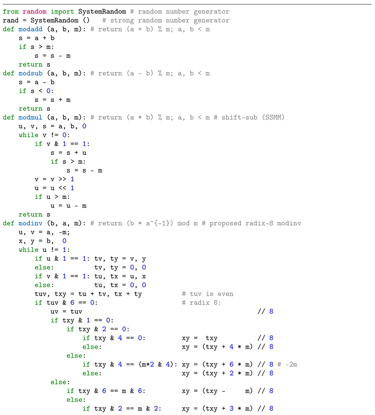
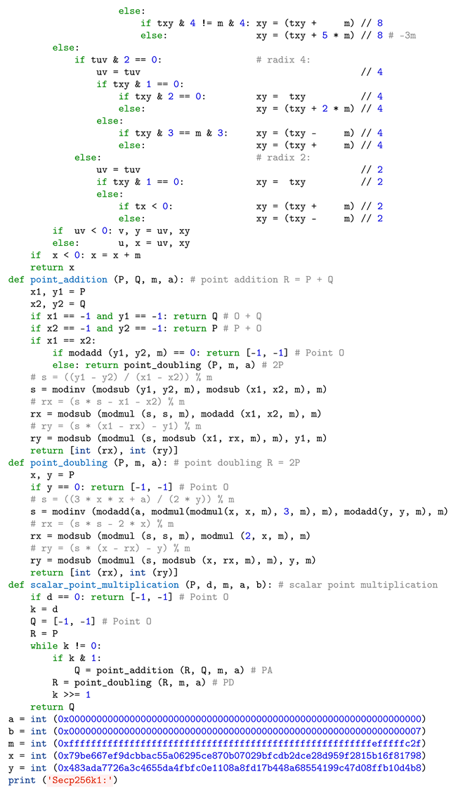
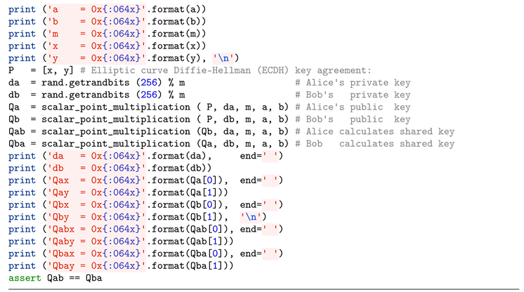
Based on the above Python code, we implemented ECC using our radix-8 modular inversion algorithm for calculating in PA and PD. Figure 4 shows the functional simulation waveform of scalar point multiplication with and . The result c is available at 635362ns. That is, the calculation takes 317681 clock cycles.
The ECC cost performance comparison is given in Table 7 when implementing on the Altera Cyclone V 5CGXFC9E7F35C8 FPGA chip. All ECC implementations use the same circuit except for the modular inversion part. Figure 5 shows the latency and AT histogram. The ECC latency using our proposed radix-8 modular inversion algorithm is 0.02007 second and its AT factor is 401237.93. From the table and histogram, we can see that our ECC implementation achieves a lower latency and a lower AT factor than all others.
5. Conclusions
In this paper, we proposed a mixed radix-8 modular inversion algorithm and hardware implementation based on 256-bit primes in Verilog HDL and compared its cost performance with other implementations on the Altera Cyclone V FPGA chip. The algorithm and its hardware implementation are area-time efficient with an AT factor of 8.30, which outperforms other algorithms and implementations. We also presented the cost performance of an elliptic curve cryptography implementation using the proposed modular inversion algorithm. Implementation results also show that our algorithm reduces execution time and requires fewer hardware resources than all other investigated algorithms.
Future research could include shortening the critical path and using carry-select adders and carry-save adders to speed up additions of large operands. Also, using a fixed prime m, Secp256k1 for example, we can simplify the circuit by considering only the case where the lower three bits are equal to 111 and using precomputations of , , and to speed up the radix-8 modular inversion calculations.
References
- Burton, D. The History of Mathematics / An Introduction (7th ed.); McGraw-Hill, 2011. [CrossRef]
- Hankerson, D.; Menezes, A.; Vanstone, S. Guide to Elliptic Curve Cryptography; Springer-Verlag: New York Inc, 2004. [Google Scholar] [CrossRef]
- Hossain, M.S.; Kong, Y. High-Performance FPGA Implementation of Modular Inversion over F_256 for Elliptic Curve Cryptography. 2015 IEEE International Conference on Data Science and Data Intensive Systems, 2015, pp. 169–174. [CrossRef]
- Daly, A.; Marnane, W.; Kerins, T.; Popovici, E. , Architectures and Applications for Reconfigurable Computing; Springer US: Boston, MA, 2005; pp. 219–229. doi:10.1007/1-4020-3128-9_18.Logic. In New Algorithms, Architectures and Applications for Reconfigurable Computing; Springer US: Boston, MA, 2005; Springer US: Boston, MA, 2005; pp. 219–229. [Google Scholar] [CrossRef]
- Mrabet, A.; El-Mrabet, N.; Bouallegue, B.; Mesnager, S.; Machhout, M. An efficient and scalable modular inversion/division for public key cryptosystems. 2017 International Conference on Engineering & MIS (ICEMIS), 2017, pp. 1–6. [CrossRef]
- Chen, C.; Qin, Z. Fast Algorithm and Hardware Architecture for Modular Inversion in GF(p). 2009 Second International Conference on Intelligent Networks and Intelligent Systems, 2009, pp. 43–45. [CrossRef]
- Choi, P.; Lee, M.K.; Kong, J.T.; Kim, D.K. Efficient Design and Performance Analysis of a Hardware Right-shift Binary Modular Inversion Algorithm in GF(p). Journal of Semiconductor Technology and Science 2017, 17, 425–437. [Google Scholar] [CrossRef]
- Wang, D.; Lin, Y.; Hu, J.; Zhang, C.; Zhong, Q. FPGA Implementation for Elliptic Curve Cryptography Algorithm and Circuit with High Efficiency and Low Delay for IoT Applications. Micromachines 2023, 14, 1–15. [Google Scholar] [CrossRef] [PubMed]
- Yang, D.; Dai, Z.; Li, W.; Chen, T. An Efficient ASIC Implementation of Public Key Cryptography Algorithm SM2 Based on Module Arithmetic Logic Unit. 2019 IEEE 13th International Conference on ASIC (ASICON), 2019, pp. 1–4. [CrossRef]
- Yan, X.; Li, S. Modified modular inversion algorithm for VLSI implementation. 2007 7th International Conference on ASIC, 2007, pp. 90–93. [CrossRef]
- Dong, X.; Zhang, L.; Gao, X. An Efficient FPGA Implementation of ECC Modular Inversion over F256. Proceedings of the 2nd International Conference on Cryptography, Security and Privacy, 2018, pp. 29–33. [CrossRef]
- Koblitz, N. Elliptic curve cryptosystems. Mathematics of Computation 1987, 48, 203–209. [Google Scholar]
- Miller, V.S. Use of Elliptic Curves in Cryptography. Advances in Cryptology — CRYPTO ’85 Proceedings; Springer Berlin Heidelberg: Berlin, Heidelberg, 1986; pp. 417–426. [Google Scholar]
- Certicom_Corp. Standards for Efficient Cryptography. SEC 2: Recommended Elliptic Curve Domain Parameters; http: //www.secg.org/sec2-v2.pdf, 2010. [Google Scholar]
- Barker, E.; Chen, L.; Roginsky, A.; Vassilev, A.; Davis, R. SP 800-56A Rev. 3, Recommendation for Pair-Wise Key-Establishment Schemes Using Discrete Logarithm Cryptography; National Institute of Standards and Technology, 2018. https://nvlpubs.nist.gov/nistpubs/SpecialPublications/NIST.SP.800-56Ar3.pdf.
- Li, Y.; Chu, W. Shift-Sub Modular Multiplication Algorithm and Hardware Implementation for RSA Cryptography. 17th International Conference on Information Assurance and Security, Lecture Notes in Networks and Systems; Springer: Cham, 2021; pp. 541–552. [Google Scholar] [CrossRef]
- Li, Y. Hardware Implementations of Elliptic Curve Cryptography Using Shift-Sub Based Modular Multiplication Algorithms. Cryptography 2023, 7, 1–29. [Google Scholar] [CrossRef]
Figure 1.
Block diagram of the proposed mixed radix-8 modular inversion circuit.
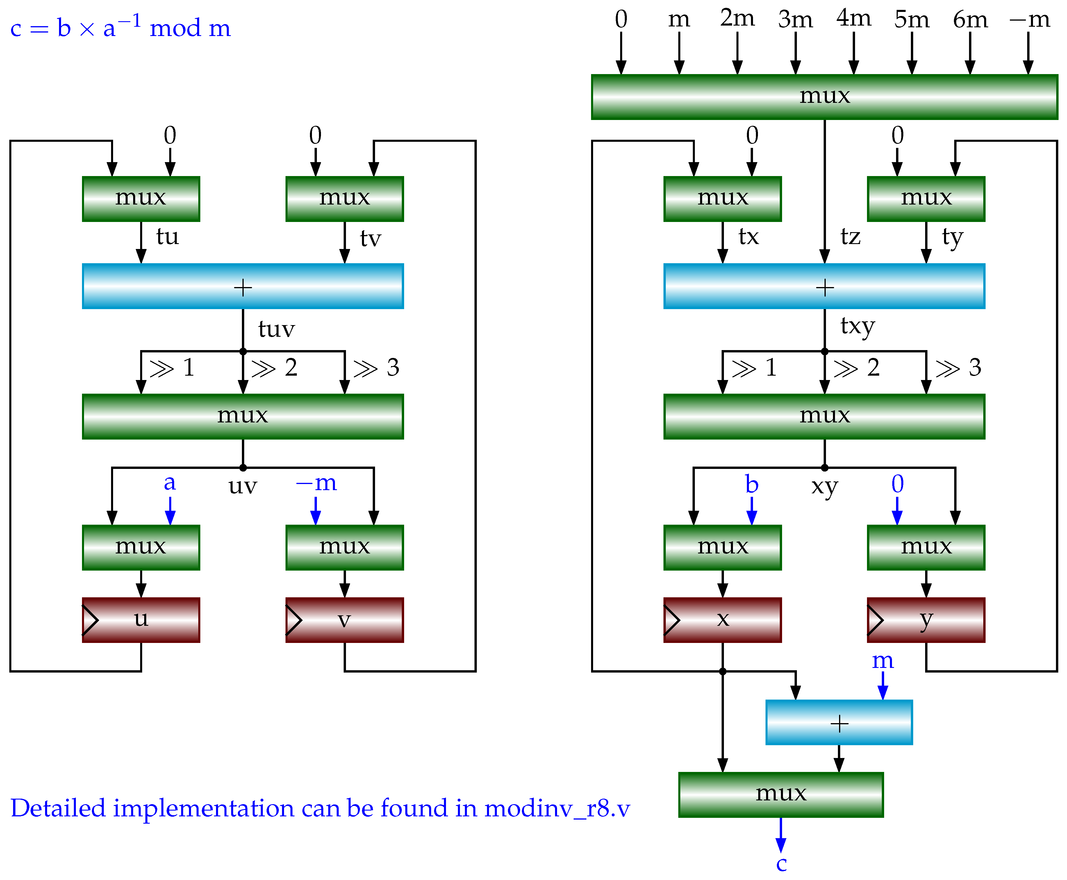
Figure 2.
Waveform of modular inversion that calculates .
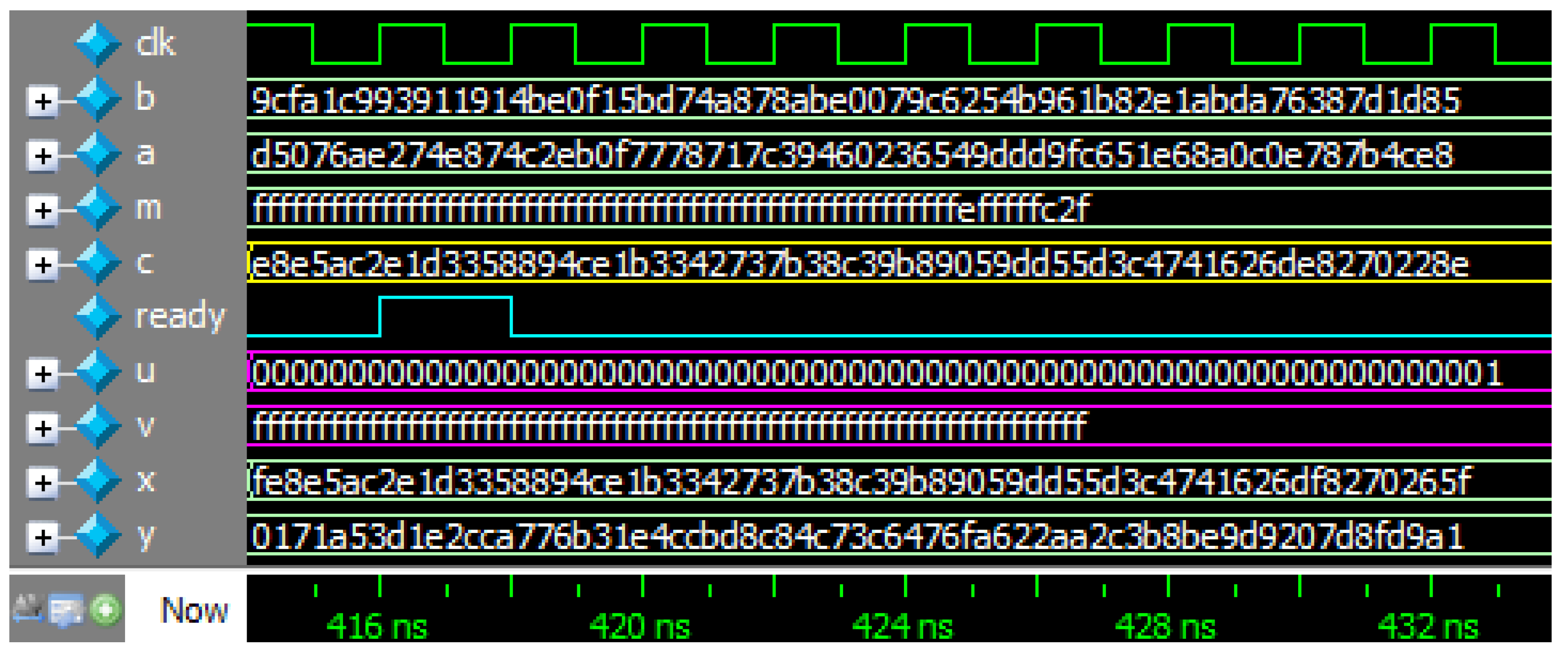
Figure 3.
Latency and AT comparison of modular inversion algorithms.
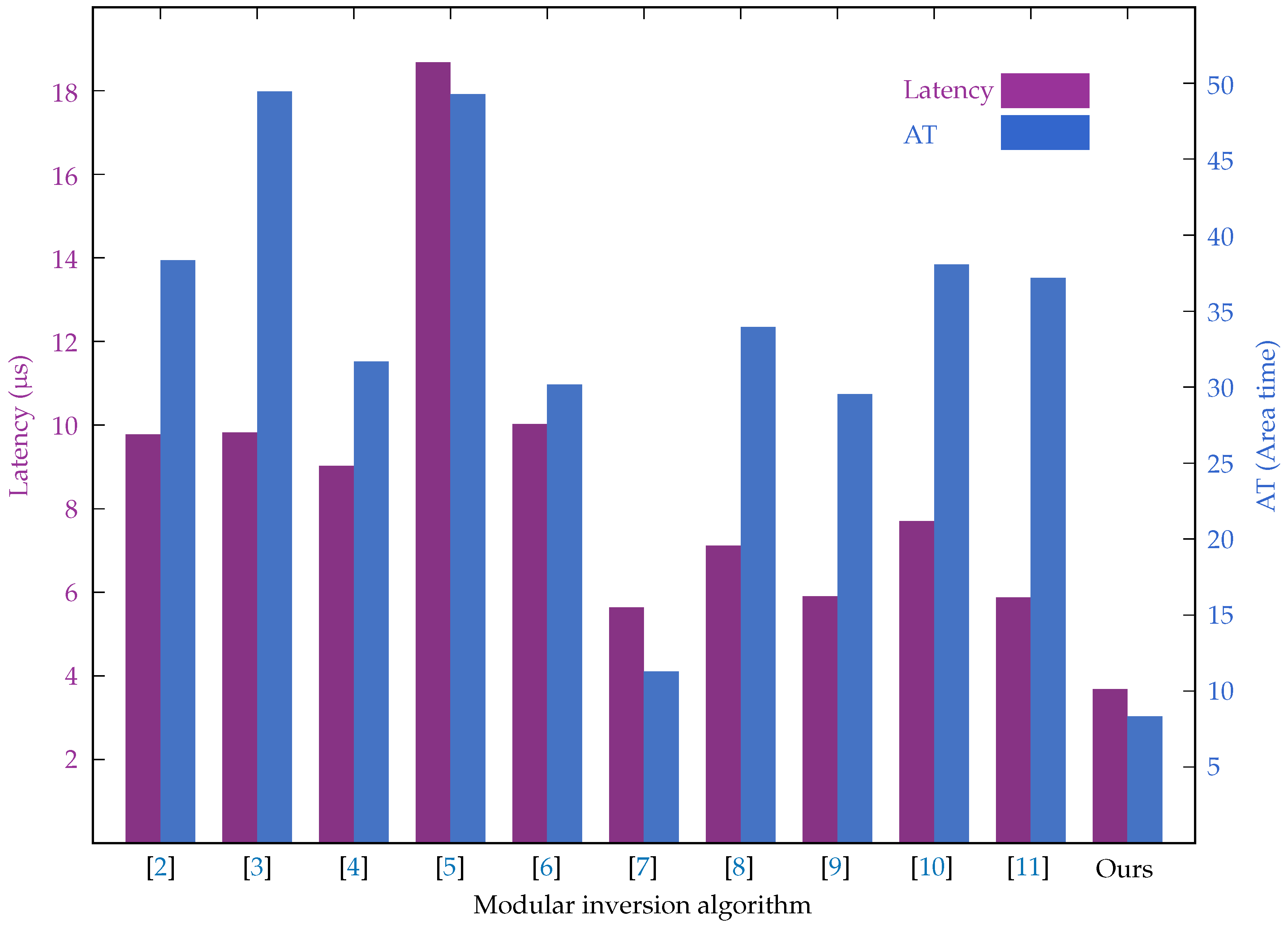
Figure 4.
Waveform of scalar point multiplication with and .
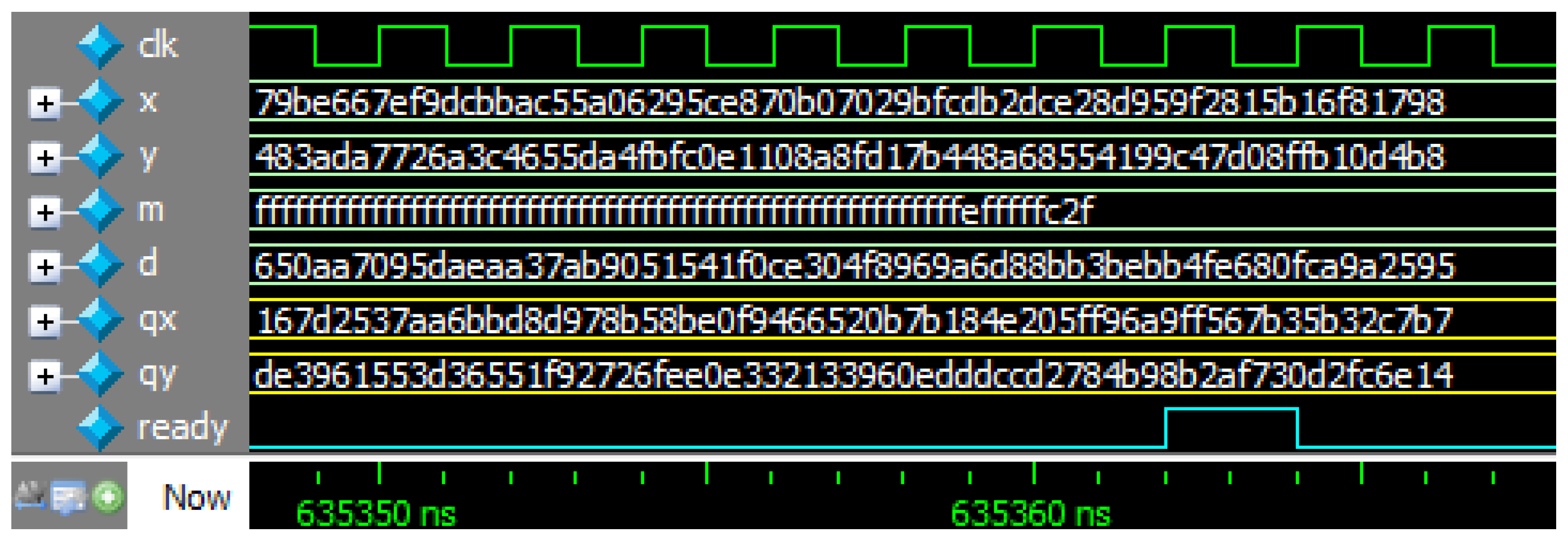
Figure 5.
ECC Latency and AT comparison of modular inversion algorithms.
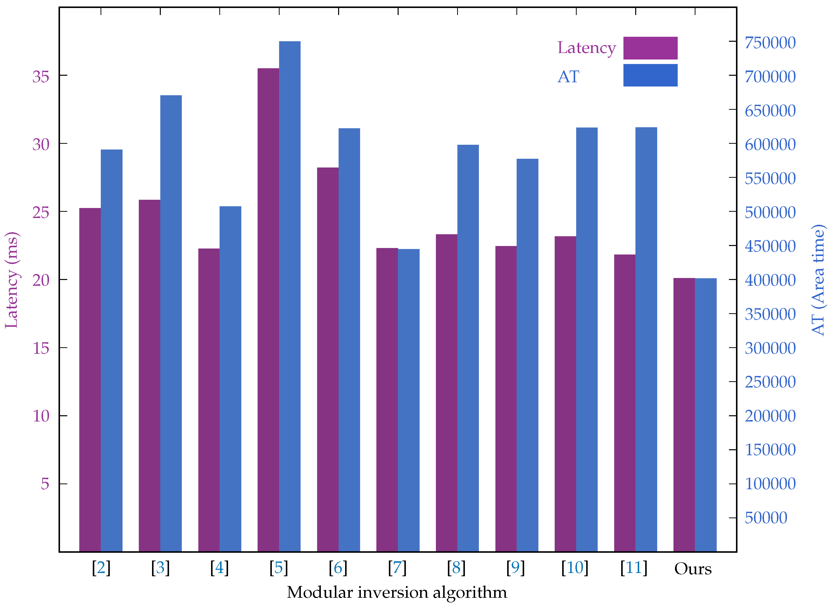

Table 1.
Elliptic curve Diffie–Hellman key exchange.
| Expose an elliptic curve and a point P on the elliptic curve to the world | |
| Alice | Bob |
| Generate a secret | Generate a secret |
| Calculate | Calculate |
| Expose | Expose |
| Get from Bob | Get from Alice |
| Calculate | Calculate |
| Use x of as the key | Use x of as the key |
Table 2.
Execution example of modinv_algo_1.py: print(modinv(1, 3, 11)). It calculates . The result is .
Table 2.
Execution example of modinv_algo_1.py: print(modinv(1, 3, 11)). It calculates . The result is .
| i | u | v | x | y | q | ||||||||||
|---|---|---|---|---|---|---|---|---|---|---|---|---|---|---|---|
| 0 | 3 | = | a | 11 | = | m | 1 | = | b | 0 | q | = | |||
| 0 | u | = | v | v | = | x | = | y | y | = | |||||
| 1 | 0 | = | |||||||||||||
| 1 | 11 | = | v | 3 | = | 0 | = | y | 1 | = | |||||
| 2 | 3 | = | |||||||||||||
| 2 | 3 | = | v | 2 | = | 1 | = | y | = | ||||||
| 3 | 1 | = | |||||||||||||
| 3 | 2 | = | v | 1 | = | = | y | 4 | = | ||||||
| 4 | 2 | = | |||||||||||||
| 4 | 1 | = | v | 0 | = | 4 | = | y | = | ||||||
| End | u | = | 1 | v | = | 0 | x | = | 4 | ||||||
Table 3.
XY adjustment for shift right by three-bit in the proposed modular inversion algorithm.
| m | Comment | |||||
|---|---|---|---|---|---|---|
| 000 | xx1 | |||||
| 100 | xx1 | 100 | ||||
| 010 | x01 | 010 | ||||
| 110 | x11 | 110 | ||||
| 010 | x11 | 110 | ||||
| 110 | x01 | 010 | ||||
| 001 | 001 | |||||
| 011 | 011 | |||||
| 101 | 101 | |||||
| 111 | 111 | |||||
| 001 | 101 | 010 | 111 | |||
| 011 | 111 | 110 | 101 | |||
| 101 | 001 | 010 | 011 | |||
| 111 | 011 | 110 | 001 | |||
| 001 | 111 | |||||
| 011 | 101 | |||||
| 101 | 011 | |||||
| 111 | 001 | |||||
| 001 | 011 | 110 | 001 | |||
| 011 | 001 | 010 | 011 | |||
| 101 | 111 | 110 | 101 | |||
| 111 | 101 | 010 | 111 |
Table 4.
XY adjustment for shift right by two-bit in the proposed modular inversion algorithm.
| m | Comment | |||
|---|---|---|---|---|
| 00 | x1 | |||
| 10 | x1 | 10 | ||
| 01 | 01 | |||
| 11 | 11 | |||
| 01 | 11 | |||
| 11 | 01 |
Table 5.
Comparison of modular inversion algorithms (on Altera Cyclone V FPGA chip).
| Algorithm | Cycles | Freq.(MHz) | Latency(s) | ALMs | Registers | AT |
|---|---|---|---|---|---|---|
| [1] | 66264 | 57.54 | 1151.6399 | 2004 | 2775 | 5503.66 |
| [2] | 66534 | 54.66 | 1219.7799 | 2619 | 1302 | 38.31 |
| [3] | 66535 | 54.52 | 1219.8199 | 3735 | 1303 | 49.42 |
| [4] | 66358 | 39.73 | 1219.0199 | 2474 | 1038 | 31.64 |
| [5] | 61205 | 64.55 | 1218.6799 | 1596 | 1043 | 49.26 |
| [6] | 66723 | 72.21 | 1210.0199 | 1968 | 1042 | 30.13 |
| [7] | 66358 | 63.60 | 1215.6399 | 959 | 1037 | 11.24 |
| [8] | 66423 | 59.56 | 1217.1099 | 3475 | 1303 | 33.92 |
| [9] | 66356 | 60.43 | 1215.8999 | 3950 | 1057 | 29.50 |
| [10] | 66423 | 54.99 | 1217.6999 | 3644 | 1303 | 38.05 |
| [11] | 66334 | 56.93 | 1215.8799 | 5276 | 1057 | 37.15 |
| Ours | 66208 | 56.71 | 1213.6799 | 1227 | 1037 | 38.30 |
Table 6.
Execution example of with .
| Weight | Point addition | Point doubling | |
|---|---|---|---|
| Initial | |||
| 1 | |||
| 2 | |||
| 4 | |||
| 8 | |||
| 16 |
Table 7.
ECC comparison using modular inversion algorithms (on Altera Cyclone V FPGA chip).
| Algorithm | Cycles | Freq.(MHz) | Latency(ms) | ALMs | Registers | AT |
|---|---|---|---|---|---|---|
| [2] | 402145 | 15.94 | 25.23 | 15043 | 8355 | 590300.42 |
| [3] | 402400 | 15.58 | 25.83 | 17585 | 8355 | 669977.92 |
| [4] | 357262 | 16.06 | 22.25 | 14975 | 7821 | 507107.38 |
| [5] | 570142 | 16.07 | 35.48 | 13292 | 7834 | 749522.08 |
| [6] | 455425 | 16.15 | 28.20 | 14211 | 7831 | 621577.58 |
| [7] | 356878 | 16.01 | 22.29 | 12114 | 7820 | 444347.67 |
| [8] | 372127 | 15.98 | 23.29 | 17292 | 8353 | 597196.30 |
| [9] | 352761 | 15.72 | 22.44 | 17841 | 7860 | 576737.31 |
| [10] | 372127 | 16.08 | 23.14 | 18548 | 8355 | 622595.32 |
| [11] | 346194 | 15.88 | 21.80 | 20716 | 7859 | 622952.99 |
| Ours | 317681 | 15.82 | 20.08 | 12157 | 7824 | 401237.93 |
Disclaimer/Publisher’s Note: The statements, opinions and data contained in all publications are solely those of the individual author(s) and contributor(s) and not of MDPI and/or the editor(s). MDPI and/or the editor(s) disclaim responsibility for any injury to people or property resulting from any ideas, methods, instructions or products referred to in the content. |
© 2024 by the authors. Licensee MDPI, Basel, Switzerland. This article is an open access article distributed under the terms and conditions of the Creative Commons Attribution (CC BY) license (http://creativecommons.org/licenses/by/4.0/).
Copyright: This open access article is published under a Creative Commons CC BY 4.0 license, which permit the free download, distribution, and reuse, provided that the author and preprint are cited in any reuse.