Submitted:
09 September 2024
Posted:
10 September 2024
You are already at the latest version
Abstract
The last wave of Artificial Intelligence is dedicating particular emphasis to the line of
explainability research. The potential of Explainable Artificial Intelligence (XAI) in producing
trustworthy computer-aided-diagnosis systems and its usage for knowledge discovery are collecting
interest in the Medical Imaging (MI) community to support the diagnostic process and the discovery
of image biomarkers. Most of the existing XAI applications in MI were focused on interpreting
the predictions returned by deep neural networks, typically including attribution techniques with
saliency map approaches and other feature visualization methods. However, these are often criticized
for providing incorrect and incomplete representations of the black-box models’ behaviour. This
raises the attention in proposing models intentionally designed to be self-explanatory. In particular,
part-prototype (PP) models are interpretable-by-design computer vision (CV) models that base their
decision process in learning and identifying representative prototypical parts from the input images,
and they are collecting increasing interest and results in MI applications. This narrative review
provides a summary of existing PP networks, their application in MI analysis and current challenges.
Keywords:
Deep Learning
; XAI
; Interpretability-by-Design
; Part-prototypes Models
; Medical Imaging
1. Introduction
Machine and Deep Learning (ML and DL) models are collecting interesting performances in supporting Medical Imaging (MI) analysis, but their black-box nature poses technical, ethical and legal controversy in this high-stakes domain. In this scenario, Explainable Artificial Intelligence (XAI) offers many opportunities to foster the development of responsible and trustworthy AI systems for healthcare applications [1,2,3,4,5].
The last decades of ML explainability research were mainly focused on developing methods for explaining complex black-box models (post-hoc interpretability), which typically include saliency-based visual methods [2,3,4]. Saliency approaches exploit the spatial information, preserved through the convolutional layers of DL models, to analyse which parts of an image lead to a resulting decision. However, these methods are often criticized for providing incorrect and incomplete representations of the black-box models’ behaviour, and explanations not fully interpretable for a human user [5,6,7,8].
To overcome the limits reported by post-hoc XAI, a most recent trend started proposing models intentionally designed to be self-explanatory (ante-hoc interpretability, or interpretability-by-design). This includes low-level complexity ML models e.g., decision tree, but also black-box methods augmented with explainability methods [1,4].
Authors started developing DL architectures known as Part-Prototype (PP) neural networks (also known as self-explaining neural networks) that perform image classification based on the identification of class-representative prototypical parts in the input image, a reasoning process based on the recognition-by-components theory [8,9]. PP networks are self-explaining models which reproduce the human case-based reasoning process, and their explanations are faithful representations of the computations performed by the model to make its decisions [6,8,10].
A PP neural network is generally constituted by a deep neural network backbone trained to learn prototypical parts. This feature extractor is trained only using image-level labels (no additional image sub-annotations are required). Once trained, the PP model classifies an input image by detecting the image patches more similar to the learned prototypical parts. The model’s interpretability is provided thanks to the transparent reasoning process implemented in the form of “this looks like that", and the direct relation between the prototypes and the classification prevents unfaithful explanation [8,10,11,12]. A representative example of the PP Net reasoning process is reported in Figure 1.
Following the XAI taxonomy [5], a PP Net can provide both global (overall model’s behaviour) and local (relative to a certain prediction) explanations by respectively showing all the learned prototypes and the detected prototypes for the given prediction as shown in Figure 2.
In addition to designing explainable models, also properly evaluating XAI is crucial to promote their application in real-world scenarios [5]. The evaluation process of XAI methods is currently an open challenge, and several works started proposing systematic evaluation frameworks to objectively assess the system developed [1,13,14]. Aspects such as the XAI multidisciplinarity and the absence of a gold standard “good explanation" make the interpretability assessment a non-trivial task, and is still not clear how XAI methods -including PP-Nets- should be evaluated [5].
This narrative review provides a summary of existing PP networks, their application in MI analysis and their current open challenges.
2. Baseline Prototypical-Part Models
There are different PP model variants proposed to date in literature [8,15], including ProtoPNet [10], XProtoNet [16], ProtoTree [17], ProtoPShare [18], ProtoPool [19], and PIPNet [8]. This section aims to summarize the main theoretical characteristics of the existing PP-nets. For each network, we will describe the architecture, training process, and visualization of the prototypical parts as patches of the input images.
2.1. Prototypical Part Network (ProtoPNet)
2.1.1. Architecture
ProtoPNet [10] was the first PP network proposed in the CV domain. ProtoPNet architecture is composed by a (1) CNN backbone f with parameters ; a (2) prototype layer of M prototypes ; and a final (3) fully connected layer h with weight .
We reported the ProtoPNet architecture in Figure 3.
The CNN backbone takes an input image and returns as output the extracted features with dimension . This could be any available CNN’s feature extractor, such as pre-trained architectures like VGG-16, VGG-19, ResNet-34, ResNet-152, DenseNet-121, or DenseNet-161.
The network learns M prototypes of shape , where , . Every prototype represents an activation pattern of the convolutional output, corresponding to a certain prototypical image patch in the original pixel space. In this way, a prototype is the latent representation of a certain image prototypical part. The prototype layer performs the computation reported in eq. (1). It evaluates the squared distances between the th prototype and patches of z with the same shape as . These distances are inverted to produce an activation map of similarity score, which indicates how strong a prototypical part is present in the image. Finally, a global max pooling of every prototype’s activation map returns a similarity score which indicates how strongly a prototypical part is present in some patch of the input image (eq. 1). The model requires the allocation of a pre-determined number of prototypes for each class , and the subset of prototypes associated with class k should capture the most relevant parts for identifying images of that class.
The last fully connected layer h multiplies the m similarity scores by the weight matrix to produce the output logits, which are finally normalized with a softmax function to obtain the class probabilities. The weight corresponds to the connection between the output of a class prototype unit and the logit of class k. Here, a positive (and respectively a negative) connection between prototype j and class k means that the similarity to a class prototype j increases (decreases) the probability that the image belongs to class k.
2.1.2. Training
The ProtoPNet training process requires three main steps: (1) Optimization of the convolutional and prototype layers; (2) Prototypes’ projection; (3) Convex optimization of the fully connected layer.
The backbone and prototype layers’ optimization (1) aims to learn a meaningful latent space, where the most important patches for classifying images are clustered (in L2-distance) around semantically similar prototypes of the images’ true classes; and the clusters of different classes are well-separated. The weights of CNN backbone and the prototypes layer are jointly optimized using stochastic gradient descent (SGD), while the weights of fully connected layer are fixed and set to:
In this way, the similarity to a prototype (not) of class k (decreases) increases the predicted probability that the image belongs to class k. SDG optimizes the following loss function:
Where:
- Cross entropy loss, penalizes misclassification on the training data.
- Cluster cost, promotes every training image to have some latent patch that is close to at least one prototype of its own class.
- Separation cost, promotes every latent patch of a training image to stay away from the prototypes not of its class.
With the prototypes’ projection (2) every prototype is projected onto the nearest latent training patch of a training image of the same class. After projection, a prototype corresponds to some patch of the latent representation , of an image in the training set .
where .
The fully connected layer optimization (3) adjusts connections from similarity score and the logit of class to enhance sparsity:
that is for k and j with we have . In doing so, we foster the model in implementing a positive reasoning process (use prototypes which add evidence for a class, not the ones whose presence decreases the evidence for the class), and further improve accuracy without changing the learned latent space or prototypes.
2.1.3. Prototypes’ visualization
Once the ProtoPNet is trained, we can visualize every prototype as a patch of an image in the training set. This visualization process involves the following steps:
- Forwarding through a ProtoPNet to produce the activation map associated with the prototypes
- Upsampling the activation map to the dimension of the input image
- Localizing the smallest rectangular patch whose corresponding activation is at least as large as the 95th-percentile of all activation values in that same map
We schematically reported the visualization process in Figure 4.
2.2. XProtoNet
XProtoNet differs from ProtoPNet due to the ability to learn representative features within a dynamic area.
2.2.1. Architecture
XProtoNet is composed by a (1) Feature extractor with two main modules: a (1.a) Feature module F and a (1.b) Occurrence module ; a (2) Similarity score measurement; and a final (3) Fully connected layer.
XProtoNet takes an input image and extracts the feature vector for each one of the learned prototypes per class with .
Where denotes the spatial location of and . The feature module extracts the image latent representation while the occurrence module predicts an occurrence map for each prototype , which indicates where every prototype is likely to appear. The feature vector then represents a certain feature in the highly activated area of the occurrence map.
Then, XProtNet uses the cosine similarity to compute a similarity score between the feature of the input image to every prototype:
Finally, every prototype contributes to the prediction score of the related class with an importance determined by the weights of the linear layer .
Where is a sigmoid activation function.
2.2.2. Training
XProtoNet follows the ProtoPNet training scheme (backbone and prototypes optimization; prototypes projection; fully connected layer optimization). Its cost function is composed by three different terms:
Where:
-
Classification weighted loss, to address the imbalance in the dataset:Where is the prediction score of the th sample , is a parameter for class balance, and the number of negative and positive labels on disease c, and the target label of on disease c.
- Regularization for Interpretability which, similarly to [10], includes two different terms and to respectively maximize similarity between x and for positive samples and minimize it for negative samples:
-
Regularization for the occurrence map:Where:
- –
- The term considers that an affine transformation of an image does not change the relative location, so it shouldn’t affect the occurrence map, either
- –
- The term regularize to have an occurrence area as small as possible to not include unnecessary regions
Once the model is trained, the prototype is replaced with the most similar feature vector from the training images.
2.2.3. Protypes’ Visualization
The learned prototypes are visualized by:
- Upsampling the occurrence maps to the input image size
- Normalizing with the maximum value of the upsampled mask
- Marking with contour the occurrence values are greater than a factor of 0.3 of the maximum intensity
2.3. Neural Prototype Tree (ProtoTree)
Nauta et al. [17] developed Neural Protype Tree (ProtoTree), which integrates the prototype learning approach into a hierarchical decision tree structure. The model includes a CNN followed by a binary tree structure, where each node corresponds to a prototypical part. The prototypical parts are tensors that can be visualized as a patch of a training sample learned with backpropagation during the training process, without requiring additional annotations. Similarly to PP network, the ProtoTree architecture itself explains the global reasoning process implemented (here, as a hierarchical sequence of steps), and the local explanations are constituted by the route through the tree for every single prediction.
2.3.1. Architecture
ProtoTree consists of a (1) CNN backbone f with parameters ; a (2) binary soft decision tree constituted of nodes, leaves, and edges, which takes the image latent representation and returns the class probability distribution over the K classes.
The CNN backbone takes the input image and extract the latent features consisting of D 2-dim feature maps, .
The binary soft decision tree takes as input the image latent representation and returns the class probability distribution over the K classes . Each internal node has two children and connected respectively with and corresponds to a prototype . Here, a prototype is a trainable tensor of shape , with the same depth as the convolutional output and . The prototype acts as a kernel which slides over , computes the Euclidean distance between and its receptive field and applies a minimum pooling to select the patch closest to :
The selected closest patch is then routed through both edges (soft routing) of child nodes with:
So, the similarity between and determines to which extent is routed to the right node child . Each leaf node receives the convolutional output with a probability given by the product of the edges probabilities in the path followed by from the root node to leaf l:
Each leaf has a trainable parameter which denotes the class probability distribution over the K classes and computes the class probability distribution of leaf l applying the softmax normalization . The class probability distribution over the K classes is given by the weighted contribution of all the leaves.
2.3.2. Training
The ProtoTree’s architecture is initialized by selecting a pre-trained CNN backbone and defining the maximum height h of the binary tree, which determines the number of prototypes . Then, the training process is constituted by the (1) Optimization of the convolutional and prototype layers; (2) Convex optimization of the decision tree’s leaves; and (3) Prototypes’ projection.
The CNN backbone and prototype layers’ are optimized (1) with backpropagation gradient descent by minimizing the cross-entropy loss between the predicted class probability distribution and ground-truth .
The convex optimization of (2) learns the leaves’ distribution using a derivative-free approach
Where t indexes a training epoch.
Finally, with the prototypes’ projection (3) every prototype is replaced with its nearest latent patch present in the training data :
Once trained, ProtoTree has a pruning step to prone ineffective prototypes reducing the explanation’s sizes, which brings benefit to the model’s interpretability. This consists of removing leaves with nearly uniform distributions, signs of little discriminative power between classes, by defining a threshold slightly greater than and pruning the ones where .
2.3.3. Prototypes’ Visualization:
Considering as the training image corresponding to the latent patch , the prototype is visualized as a patch of by:
- Forwarding through
-
Create a 2-dim similarity map:Where denotes the location of patch in patches of z
- Upsampling with bicubic interpolation to the shape of
- Visualize as a rectangular patch at the same location nearest to the latent patch
2.4. Protypical Part Shared Network (ProtoPShare)
Rymarczyk et al. [18] developed ProtoPShare, a part-prototype network which extended ProtoPNet addressing two of its limitations: the (1) Ability to share prototypes between the classes; the (2) Ability to identify semantically similar prototypes, even with a distant representation in the latent space. The authors achieved this by implementing a data-dependent pruning algorithm based on the feature maps. This results in a model with a reduced explanation size, fostering its interpretability.
2.4.1. Architecture
ProtoPShare shared the same architecture as ProtoPNet constituted of a CNN backbone f extracting the latent representation of the image ; a prototype layer g of prototypes per classes ; and a fully connected layer of weight which predicts the output class.
2.4.2. Training
ProtoPShared adopted the ProtoPNet training scheme followed by a data-dependent merge-pruning to obtain a network with a smaller number of shared prototypes. The pruning process consists of the following steps:
- Computing the data-dependent similarity for pair of prototypes , given by the compliance on the similarity scores for all the training input image . This considers two prototypes similar if they activate alike on the training images, even if far in the latent space:
- Select a percentage of the most similar pairs of prototypes to merge per step
- For each pair, remove prototype and its weights and reuses prototype aggregating weights and
Results obtained compared to other self-explained prototypical parts models suggested an increase in interpretability and a novel ability to discover semantic similarity discovery while maintaining high accuracy.
2.4.3. Prototypes’ Visualization
As ProtoPNet [10], the visualization process of the prototypes is based on the localization of the smallest and most activated rectangular patch in the upsampled image activation map.
2.5. ProtoPool
Rymarczyk et al. [19] developed ProtoPool integrating into PP-network (1) the concept of prototypes soft assignment, which optimizes for model’s compactness without requiring a pruning stage into the training process; and (2) the definition of focal similarity function to focus the model on salient features. As ProtoPShare [18], the prototypes can be shared between classes.
2.5.1. Architecture
ProtoPool shared the same architecture as ProtoPNet constituted of a CNN backbone f; a prototype layer g of m prototypes ; and a fully connected layer of weight which predicts the output class.
The image latent representation with dimension is considered as a set of vectors each one corresponding to a location in the image and with dimension D: .
The prototype layer contains K slots for each class, and each slot is implemented as a distribution of the prototypes in the pool where is the probability of assigning successive prototypes to the slot. The layer computes on each k slot the aggregated similarity between and all prototypes considering their slot distribution :
Here, ProtoPool computes the activation of prototype p w.r.t. image x using the novel-introduced focal similarity function:
Where:
The focal similarity has the advantage of preventing: high activation due to all the elements in are similar to a prototype, which might result in obtaining prototypes focused on the background regions, and the gradient is passed only through the most active part of the image. ProtoPool also uses the concept of soft assignment on prototype distributions, applying the Gumbel-softmax estimator to avoid many prototypes being assigned to one slot (which might decrease interpretability):
Where:
Where for are sampled from the standard Gumbel distribution.
2.5.2. Training
ProtoPool adopted the ProtoPNet training scheme (backbone and prototype training; prototypes projection; backbone, prototypes and fully connected layer fine-tuning) by extending the loss function to avoid that the same prototype will be assigned to many slots of one class:
As in ProtoPNet, the prototypes are projected to replace every learned abstract prototype with the representation of the nearest training patch:
Where ; here, differently from ProtoPNet, C is the set of all the classes assigned to prototype p.
2.5.3. Prototypes’ Visualization
Even for ProtoPool, the visualization process of the prototypes is based on the upsampling of the activation maps as in ProtoPNet [10].
2.6. Patch-based Intuitive Prototypes Network (PIPNet)
Nauta et al. [8] developed a Part-Prototype architecture which presents different advantages compared to the existing models: (1) Absence of semantic gap between the learned prototypes and human vision; (2) Compactness; and (3) Ability to handle Out-of-Distribution (OoD) data.
The lack of semantic gap means that the prototypes learned correlate with human concepts, ground-truth object parts and human visual perception. This was covered by implementing an extra regularization of the prototypes using Self-supervised Representation Learning. PIPNet overcomes the assumption that part of the images from the same class have the same prototypes (regularization of interpretability at the class level).
The model’s compactness was promoted by regularizing for sparsity during training of the weights in the fully connected layer between prototypes and classes. PIP-Net only needs an upper bound on the number of prototypes selecting as few prototypes as possible for good classification accuracy and allowing class-sharable prototypes This regularization was performed by introducing a novel function that optimizes classification performances and compactness simultaneously, which is also able to handle OoD data.
Finally, PIP-Net manages OoD data by abstain from decisions when no relevant prototypes are present in the image. This was implemented enabling the assignment of near-zero scores for all classes using a normalization (necessary for scale-invariance issues) in logits where a score of zero stays zero and allows the prototype presence score to behave independently of each other.
2.6.1. Architecture
PIP-Net consists of a (1) CNN backbone f with parameters followed by a softmax activation; a (2) Global Max-pooling operation extracting the prototype layer ; and a final positive sparse (3) fully connected layer which acts as a scoring sheet system to predict the output classes. PIP-Net classifies images based on the presence of prototypical parts in the input image. The relevantly present prototypical parts add up scores (evidence) to the model’s classes with a proportional contribution determined by the linear weights and the model can abstain from decisions when there isn’t enough evidence for any classes.
The CNN backbone takes the input image and extract the latent features consisting of D 2-dim feature maps, . The softmax activation normalizes so that . Here represents the probability that a patch in position corresponds to the prototype d, that is, the one-hot encoding of patch to the prototype d.
The global max-pooling 2D operation extracts D prototypes and calculates the prototypes presence scores where , where measures the presence of the prototype d in the input image.
Finally, a linear sparse classification layer with positive weights connects the prototypes to the classes acting as a scoring sheet systems: with is and , where represents the contribution of prototype d for class k.
2.6.2. Training
The PIPNet training process is composed of two main steps: the (1) Self-Supervised Pre-Training of Prototypes; and the (2) PIP-Net training.
The prototypes’ pre-training aims to learn an image encoding p with semantic similarity independently from the classification task (the last linear layer is kept frozen). Authors optimize for patch alignment under a contrastive learning approach by training PIP-Net to assign the same prototypes to two views of an augmented image patch. This involves a positive pair creation step by applying data augmentation transformation to input image x selected so that humans consider the two views similar. The Adam optimizer optimizes the following loss function:
Where:
-
Alignment Loss, optimizes for near-binary encodings where an image patch corresponds to exactly one prototypeWhere the dot product assess the similarity between the latent patches of two views of an image patch, if
- Tanh-Loss, prevents the trivial solution that one prototype node is activated on all image patches in each image in the dataset forcing that every prototype should be at least once present in a mini-batch
The PIPNet training optimizes classification performances and fine-tunes the prototypes for the downstream classification task.
Where the Classification Loss, , is the Log-likelihood loss between the ground-truth labels and the predictions During training, the output scores are computed as , acting as regularization for sparsity.
2.6.3. Prototypes’ Visualization
The visualization process of the prototypes is based on the upsampling of the latent output based on the single most activated latent patch.
3. Application and Advances in Medical Imaging
There is an increasing interest in applying PP model in medical imaging. We searched in major databases (Google Scholar, Scopus, Web of Science) articles including original research papers and preprints on PP networks applied in medical image classification published from 2019 to August 2024. We summarized collected works in Table 1.
Singh et al. proposed three ProtoPNet variants for classifying chest images into Covid-19, Pneumonia and Normal: Negative-Positive ProtoPNet (NP-ProtoPNet) [20], Generalized ProtoPNet (Gen-ProtoPNet) [21], and Pseudo-ProtoPNet (Ps-ProtoPNet) [22]. In NP-ProtoPNet [20] authors modified the original fully connected layer by connecting similarity scores to correct/incorrect classes’ logits with weights fixed respectively to 1 or -1. This allows the network to reason both in a “positive” way (“this looks like that”) and in a “negative” way (“this does not look like those”), i.e., by exclusion. In Gen-ProtoPNet [21] authors introduced a generalized distance function to select prototypes of varying dimensions. They achieved accuracies of 88.99% in the first work and of 87.27% in the second. They also trained black-box CNNs for the same task, showing that their explainable models’ performances are comparable with state-of-the-art (SOTA) black-box models. For both works, they used a combination of two datasets, one containing frontal chest radiographs of healthy people and pneumonia patients (Chest X-ray [23]), and the COVID-19 Image Data Collection [24], from which they took radiographs of COVID patients. The Ps-ProtoPNet [22] integrates NP-ProtoPNet and Gen-ProtoPNet. For this implementation, they used CT images from COVIDx CT-2 Dataset available on Kaggle, achieving an accuracy of 99.24%
- Kim et al. [16] implemented X-ProtoPNet, which introduces the prediction of occurrence maps, which indicate the area where a sign of the disease (i.e., a prototype) is likely to appear, so compares the features in the predicted area with the prototypes. This novelty can help to identify whether the model is focusing on the correct parts of the image or if it is being misled by irrelevant features. They used the NIH chest X-ray dataset [25] for a multilabel classification task (Atelectasis, Cardiomegaly, Effusion, Infiltration, Mass, Nodule, Pneumonia, Pneumathorax Consolidation, Edema, Emphysema, Fibrosis, Pleural Thickening, and Hernia), achieving a mean area under the receiver operating characteristic (AUROC) of 0.822.
- Mohammadjafari et al. [26] applied ProtoPNet to brain MRI scans to detect Alzheimer’s disease, achieving an accuracy of 87.17% in the OASIS dataset [27] and of 91.02% in the ADNI dataset. They used different CNN architectures as feature extractors, and ProtoPNet’s performances were demonstrated to be comparable to or slightly less than their black-box counterparts.
- Barnett et al. [28] designed a novel PP net modifying the training process of ProtoPNet with a loss function including fine-grade expert image annotation and using a top-k average pooling instead max-pooling. They trained their model on an internal dataset of digital mammograms for mass-margin classification and mass-margin malignancy prediction and reported equal or higher accuracy compared to PrototPNet and a black-box model.
- Carloni et al. [29] used ProtoPNet to classify benign/malignant breast masses from mammogram images from a publicly available dataset (CBIS-DDSM [30]), achieving an accuracy of 68.5%. While this performance may not yet be ideal for clinical practice, the authors suggest three tasks for a qualitative evaluation of the explanations by a radiologist.
- Amorim et al. [31] implemented ProtoPNet to classify histologic patches from the PatchCamelyon dataset [32] into benign and malignant using a top-k average pooling instead a max-pooling to extract similarity scores from the activation maps. The authors achieved an accuracy of 98.14% by using Densenet-121 as a feature extractor. This performance was comparable with the one obtained with the black-box CNN.
- Flores-Araiza et al. [33] used ProtoPNet to identify the type of kidney stones (Whewellite, Weddellite, Uric Acid anhydrous, Struvite, Brushite and Cystine) using a simulated in-vivo dataset of endoscopic images. They achieved an accuracy of 88.21% and further evaluated the explanations by perturbing global visual characteristics of images (hue, texture, contrast, shape, brightness, and saturation) to describe their relevance to the prototypes and the sensitivity of the model.
- Kong et al. [34] designed a dual-path PP network, DP-ProtoNet, to increase the generalization performances of single networks. They applied their model to the public ISIC - HAM10000 skin disease dermatoscopic dataset [35]. Compared to ProtoPNet, DP-ProtoNet achieved higher performances while maintaining the model’s interpretability.
- Santiago et al. [36] integrated ProtoPNet with content-based image-retrieval to provide explanations in terms of image-level prototypes and patch-level prototypes. They applied their approach to the skin lesions diagnosis in the public ISIC dermoscopic images [35], outperforming both black-box models and SOTA explainable approaches.
- Cui et al. [37] proposed MBC-ProtoTree, an interpretable fine-grained image classification network based on ProtoTree. They improved ProtoTree by designing a multi-grained feature extraction network, a new background-prototypes removing mechanism, and a novel loss function. The improved model achieved higher classification accuracy on the Chest X-ray dataset.
- Nauta et al. [11] applied their PIP-Net to two open benchmark datasets, respectively for skin cancer diagnosis (ISIC), bone X-ray abnormality detection (MURA), and two real-world datasets respectively for hip and ankle fracture detection. From this study, authors obtained prototypes generally in line with medical knowledge and demonstrated the possibility of correcting the undesired model’s reasoning process with a human-in-the-loop configuration.
- Santos et al. [38] integrated ProtoPNet into a Deep Active Learning framework to predict diabetic retinopathy on the Messidor dataset [39]. The framework allows to train the ProtoPNet on a training set of instances selected using a search strategy, and this may offer benefits in scenarios where the datasets are expensive to be labelled. Performances reported demonstrated the success of applying interpretable models with reduced training data.
- Wang et al. [40] proposed InterNRL integrating ProtoPNet into a student-teacher framework, together with an accurate global image classifier. They applied their model for breast cancer and retinal disease diagnosis and obtained SOTA performances demonstrating the success of the reciprocal learning training paradigm in the medical imaging domain.
- Xu et al. [41] proposed a prototype-based vision transformer applied to COVID-19 classification. They replaced the last two layers of a transformer encoder with a prototype block similar to ProtoPNet and obtained good performances on three different public datasets.
- Sinhamahapatra et al. [42] proposed ProtoVerse, a PP model with a novel objective function applied to the vertebral compression fractures classification. The model interpretability was evaluated by expert radiologists, and predictive performances outperformed ProtoPNet and other SOTA PP architectures.
- Pathak et al. [15] further applied PIP-Net to three different public datasets for breast cancer classification obtaining competitive performances w.r.t. other SOTA black-box and prototype-based models and assessed the coherence of the model with quantitative metrics.
- Gallée et al. [43] applied the Proto-Caps PP-net, in lung chest CT nodules malignancy prediction and performed a human evaluation of the model with a user study.
Most of the existing PP-Nets were originally designed for general CV purposes, so they typically work by taking RGB-images as input. However, medical imaging diagnosis is often performed using the entire volumetric human anatomy, so being able to efficiently process 3D data volumes might be particularly relevant in this context. Wei et al. [44] proposed MProtoNet as the first medical prototype network extending PP models to 3D brain tumour classification from multiparametric MRI (mpMRI). This is based on an implementation of the XProtoNet with a 3D ResNet backbone and the novelty proposed soft masking and online-CAM loss function to enhance the localization of attention regions. Authors further proposed novel metrics to assess the correctness and localization coherence of prototypes (following the Co-12 taxonomy [45]). The MProtoNet obtained classification accuracy in line with the baseline CNN counterpart and ProtoPNet (re-implementated for 3D images).
Vaseli et al. [46] proposed ProtoASNet, a PP model which extracts spatio-temporal feature vectors to detect aortic stenosis from B-mode echocardiography videos. They both assessed their model on a private and on the public TMED-2 dataset [47] outperforming the baseline ProtoPNet and XProtoNet. De Santi et al. [48] extended PIP-Net to classify 3D MRI for Alzheimer’s disease. They tested the model using different CNN backbones and obtained the best result with the ResNet-18 3D, and comparable results with the corresponding black-box counterpart. They further proposed two novel quantitative metrics of explainability: the prototype brain entropy to assess the covariate complexity and localization consistency to assess the consistency in prototype localization (under the Co-12 properties). They also evaluated prototypes with domain experts with a survey and assessed the coherency of prototypes in terms of localization, pattern and classification.
Clinicians often use multiple data sources in their decision-making process [43,49], so developing explainable multimodal models (models which use multiple data sources to predict outcomes) might help in creating models which implement a decision-making process closer to a real-life application scenario. In the context of multimodality-based prototype learning, we can distinguish two main approaches in producing the prototype representation according to the way of introducing different modalities: (1) deterministic prototypes and (2) shifted prototypes [50]. The first approach typically trains different encoders for all the different modalities, then a connection layer (cross-modal encoder) concatenates the output feature vector extracted generating an unimodal vector into a joint space, used by the PP-Net to perform similarity calculation. Alternatively, some studies have introduced multimodal feature vectors to shift the prototype representations without prior fusion. Here, existing approaches leverage auxiliary modalities to enrich the embedding representation of a main modality. The shifted prototype can be explicitly modelled or their influence can be indirectly added to the objective function used to train an embedded network [50]. Most of the multimodal PP networks proposed in general CV applications integrate visual information with text data [50]. Despite being still considered a relatively unexplored field, we can also find some applications in medical imaging.

Table 1.
Part Prototype Network applied in medical imaging. Here, we reported predictive Accuracy (Acc), Balanced Accuracy (Bal Acc), and Area Under the Curve (AUC) according to the provided predictive performances.
Table 1.
Part Prototype Network applied in medical imaging. Here, we reported predictive Accuracy (Acc), Balanced Accuracy (Bal Acc), and Area Under the Curve (AUC) according to the provided predictive performances.
| Paper | Modality | Dataset | Classes | Results |
|---|---|---|---|---|
| 2D image models | ||||
| Singh et al. [20] | X-ray | Chest X-ray, COVID-19 Image |
Normal, Pneumonia, Covid-19 | Acc = 88.99% |
| Singh et al. [21] | X-ray | Chest X-ray, COVID-19 Image |
Normal, Pneumonia, Covid-19 | Acc = 87.27% |
| Singh et al. [22] | CT | COVIDx CT-2 | Normal, Pneumonia, Covid-19 | Acc = 99.24% |
| Kim et al. [16] | X-ray | NIH chest x-ray | Atelectasis, Cardiomegaly, Effusion, Infiltration, Mass, Nodule, Pneumonia, Pneumathorax, Consolidation, Edema, Emphysema, Fibrosis, Pleural Thickening, Hernia |
Mean AUC = 0.822 |
| Mohammadjafari et al. [26] | MRI | OASIS, ADNI | Normal vs. Alzheimer’s disease | Acc: 87.17% (OASIS), 91.02% (ADNI) |
| Barnett et al. [28] | Mammography | Internal dataset | Mass-margin classification Malignancy prediction |
AUC: 0.951 (Mass-margin) 0.84 (Malignancy) |
| Carloni et al. [29] | Mammography | CBIS-DDSM | Benign, malignant | Acc = 68.5% |
| Amorim et al. [31] | Histology | PatchCamelyon | Benign, malignant | Acc = 98.14% |
| Flores-Araiza et al. [33] | Endoscopy | Simulated in-vivo dataset |
Whewellite, Weddellite, Uric Acid anhydrous, Struvite, Brushite, Cystine |
Acc = 88.21% |
| Kong et al. [34] | Dermatoscopic images | ISIC - HAM10000 | Actinic keratosis intraepithelial carcinoma, Nevi, Basal cell carcinoma, Benign Keratosis-like Lesions, Dermatofibroma, Melanoma, Vascular lesions |
F1 = 74.6 |
| Santiago et al. [36] | Dermatoscopic images | ISIC - HAM10000 | Actinic keratosis intraepithelial carcinoma, Nevi, Basal cell carcinoma, Benign Keratosis-like Lesions, Dermatofibroma, Melanoma, Vascular lesions |
Bal Acc = 75.0% (Highest, achieved with DenseNet) |
| Cui et al. [37] | X-ray | Chest X-ray | Normal, Pneumonia | Acc = 91.4% |
| Nauta et al. [11] | Dermoscopic images, X-Ray |
ISIC, MURA, Hip and ankle fraction internal dataset |
Benignant, malignant, Normal, abnormal, Fracture, no fracture |
Acc: 94.1% (ISIC) 82.1% (MURA) 94.0% (Hip) 77.3% (Ankle) |
| Santos et al. [38] | Retinograph | Messidor | Healthy vs. Diseased retinopathy | AUC = 0.79 |
| Wang et al. [40] | Mammography, Retinal OCT |
Mammography internal dataset, CMMD, NEH OCT |
Cancer vs. Non-cancer Benignant vs. Malignant Normal, Drusen, and Choroidal neovascularization |
AUC = 91.49 (Internal) AUC = 89.02 (CMMD) Acc = 91.9 (NEH OCT) |
| Xu et al. [41] | X-ray Lung CT |
COVIDx CXR-3 COVID-QU-Ex Lung CT scan |
COVID-10 Normal Pneumonia |
F1: 99.2 96.8 98.5 |
| Sinhamahapatra et al. [42] | CT | VerSe’19 dataset | Fracture vs. Healthy | F1 = 75.97 |
| Pathak et al. [15] | Mammography | CBIS, VinDir, CMMD | Benignant vs. Malignant | F1 (PIP-Net model): 63±3% (CBIS) 63±3% (VinDir) 70±1% (CMMD) |
| Gallée et al. [43] | Thorax CT | LIDC-IDRI | Benignant vs. Malignant | Acc = 93.0% |
| 3D image models | ||||
| Wei et al. [44] | 3D mpMRI: T1, T1CE, T2, FLAIR | BraTS 2020 | High-grade vs. Low-grade glioma | Bal Acc = 85.8% |
| Vaseli et al. [46] | Echocardiography | Private dataset TMED-2 |
Normal vs. Mild vs. Severe Aortic Stenosis |
Acc: 80.0% (Private) 79.7 (TMED-2)% |
| De Santi et al. [48] | 3D MRI | ADNI | Normal vs. Alzheimer’s disease | Bal Acc = 82.02% |
| Multimodal models | ||||
| Wolf et al. [51] | 3D 18F-FDG PET and Tabular data | ADNI | Normal vs. Alzheimer’s disease | Bal Acc = 60.7% |
| Wang et al. [52] | Chest X-ray and reports | MIMIC-CXR | Atelectasis, Cardiomegaly, Consolidation, Edema, Enlarged Cardiomediastinum, Fracture, Lung Lesion, Lung Opacity, Pleural Effusion, Pleural Other, Pneumonia, Pneumothorax, Support Device |
Mean AUC = 0.828 |
| De Santi et al. [53] | 3D MRI and Ages | ADNI | Normal vs. Alzheimer’s disease | Bal Acc = 83.04% |
Wolf et. al [51] developed PANIC, a Prototypical Additive Neural Network for Interpretable Classification of Alzheimer’s Disease, which performs the classification Alzheimer’s Disease vs. Healthy from 3D 18F-FDG PET images integrated with tabular data. PANIC integrated the image prototypes extracted by a 3D ProtoPNet with N tabular features using an interpretable Generative Additive Model. PANIC obtained a higher balanced accuracy compared to the performances obtained with a black-box model for heterogeneous data. Wang et al. [52] proposed MProtoNet, an interpretable multimodal network which performs diagnosis using images and textual information from medical reports. The architecture combines a position embedding and a multimodal attention module applied to the chest MIMIC-CXR dataset [54], and reported improvements in predictive performances with respect to ProtoPNet without sacrificing the interpretable nature. De Santi et al. [53] proposed Patch-based Intuitive Multimodal Prototypes Network (PIMPNet), a multimodal prototype classifier which learns 3D image part-prototypes and prototypical values from structured data, to predict patient’s cognitive level in AD from sMRI and age values. They introduce the concept of age-prototypical layer to directly learn relevant age values. PIMPNet performed the classification concatenating the image prototypes extracted by a 3D PIPNet with the age prototypes using an intepretable scoring-sheet system; however, the age prototypes do not improve the predictive performance of the model trained with images only.
4. Evaluation of Prototypes
Evaluating XAI method is crucial to verify that the explanations produced are robust, sensitive to the model and data, and consistent, but this is still considered an open and developing field [5,55].
Assessing XAI outputs is considered challenging: there is still no agreement on what interpretability and explainability really are, and a general ground truth to compare explanations is missing. Researchers have proposed different evaluation frameworks to assess XAI methods, and despite there not being a a unique solution yet, most approaches agree concerning the need of considering the multidisciplinary and multidomain nature of the explanation [1]. In this scenario, including quantitative metrics to assess the technical appropriateness and reliability of explanations is crucial. To effectively capture the whole impact of XAI on supporting decision systems in real-world scenarios, is also fundamental to include the human aspect of explanation in the evaluation process [14,56]. The human evaluation should assess how explanations are perceived, their relationship with any expert-domain background knowledge, and how they affect the classification performances, and how all those aspects vary according to the presentation format of explanations.
However, while the effectiveness of post-hoc explainability methods has been investigated extensively, research lines on quantitative analysis of self-explainable approaches are still in their early stage [57]. Particularly relevant for PP-network is the general evaluation framework proposed by Nauta et al. [45]. Here, the “explainability" is considered as a non-binary characteristic, and authors developed a categorization scheme by identifying 12 conceptual properties, the so-called “Co-12 properties”. Nauta et al. [12] further applied their Co-12 evaluation strategy to PP models, providing a recipe to systematically evaluate this family of interpretable models. This overview might be particularly relevant such as most of XAI evaluation methods were designed for posthoc XAI [12,57]. We summarized the evaluation framework grouped with properties grouped by their most prominent dimension in Table 2.
Wei et al. [44] proposed two novel interpretability metrics to assess correctness and localization coherence of prototypes (following the Co-12 taxonomy [45]). The correctness was evaluated proposing the incremental deletion score (IDS) and is based on an incremental deletion process. The localization coherence was evaluated with activation precision (AP) metrics, which and assessed the intersection between the activation map and human-annotated label.
Pathak et al. [15] further developed a general framework for Coherence (one of the Co-12 properties), the so-called PEF-Coh, to quantitatively measure the quality of prototypes w.r.t. domain knowledge for breast cancer prediction from mammography. The PEF-Coh presents six metrics, whose assessment requires a dataset annotated with regions of interest: Relevance; Specialization; Uniqueness; Coverage; Class-specific; and Localization.
Gallée et al. [43] evaluated the Proto-Caps PP-net, which predicts malignancy scores in lung chest CT nodules, and provides explanations in terms of predefined image features attributes and image prototypes. They evaluated their model by performing a user study with 6 radiologists based on a survey to test how explanations affect the (1) user’s performance; (2) trust in the model and if they are (3) helpful or not. They structured a questionnaire differentiating by radiologists’ experience; assessing for the malignancy; their confidence in the prediction and the model’s output. Here, test cases were provided to the users with different levels of explainability. Finally, the questioner asked for an overall assessment of the explanations’ helpfulness. Results confirmed existing literature in observing that: (1) explanations improve performances when the model is correct, but might also convince the user of incorrect predictions; (2) the trust in the model is both influenced by the model’s accuracy and the extent of model’s reasoning; and (3) explanations are generally perceived as useful for the user.
Recent work aims to evaluate explanations using synthetic datasets. In particular, the FunnyBirds framework introduces a synthetically generated dataset of birds with concepts-parts annotation, and a set of metrics to evaluate explanations following the e Co-12 taxonomy. Opłatek et al. [58] applied the FunnyBirds framework to evaluate prototypes produced by ProtoPNet. Their results suggested that explanations provided in the form of similarity maps instead of bounding boxes provide a more faithful representation of the model, resulting in higher-quality explanations. This study further highlights the importance of considering proper visualization techniques in PP models.
The prototype evaluation process has also recently highlighted some concerns about the correctness of the spatial localization of the prototypes [57]. The visualization process of the prototypical part extracted by PP models is generally based on the upsampling of the extracted similarity maps. Despite being PP-Nets claimed to implement an inherently self-explainable case-based reasoning process, recent work reports concerns about the faithfulness of the model-agnostic upsampling process for the part-prototype visualization [57,59]. Guatam et al. [57] proposed Prototype Relevance Propagation (PRP) as a model-aware visualization strategy of prototypical part to address the main drawbacks of the PP-Net upsampling visualization: the low resolution activation maps and spatially imprecise prototype explanations. Xu et al. observed that the upsampling process may incorrectly locate parts of the images, suggesting to use of what they reported as more faithful saliency methods like SmoothGrads or PRP [59].
5. Discussion
Part-prototype networks are self-explainable methods which combine the computational power of DL into an interpretable-by-design decision-making process. PP-nets constitute a prominent solution in medical imaging analysis, where explainability is crucial to ensure the trustworthiness of the AI system, but post-hoc explainable methods reported several drawbacks in terms of reliability and completeness [5,15].
ProtoPNet is the first part-prototype network proposed to perform an interpretable imaging classification, then, other architectural variants follow it [10]. These still implement a classification using a case-based reasoning process, but differ from the first one for how combining prototypical parts to base decisions [17], for introducing the concept of class-shared prototypes [18], and addressing some of reported ProtoPNet limitations, likes the semantic gap between latent and image prototypes representations [8].
Most of PP-Net were originally designed in general CV applications and then shifted to the medical imaging domain. Integrating a deep features extractor into a PP-network often reported competitive performances compared to the fully black-box model counterparts [21,26,31], with the further potential of being able of correcting undesired reasoning process by performing a prototype suppression [11]. Medical images have already reported benefits from the general CV PP-Net; however, this domain might also require peculiar adaptation such as the ability to process 3D image scans and multimodal data domain [44,51,53].
Evaluating XAI methods, including PP-Nets, with standard quantitative frameworks is still considered an open challenge, but crucial to developing reliable and trustworthy systems. Authors generally agree that the evaluation process should be multidisciplinary and multidomain, to be able to capture the multiple aspects that characterize explanations, such as the evaluation recipee proposed by Nauta et al. [12]. Most MI applications of PP-Net performed an evaluation process including domain expert user studies and quantitative metrics. Despite the training of PP-Net does not require further annotation to the class-level labels, most of the prototype evaluation metrics proposed are based on the usage of further image-level annotations such as the segmentation of regions of interest in the images. So, the availability of sub-annotated image dataset might be also beneficial or the development of PP models. Finally, despite the general belief in considering PP-nets as reliable XAI methods due to their self-explainable nature; recent works highlighted drawbacks in the prototypes visualization based on a model-agnostic upsampling process, and proposed alternative solution to produce more spatially-accurate prototypes [57,59].
Author Contributions
Writing—review and editing, L.A.D.S., F.I.P., F.B., M.F.S., V.P.; supervision, S.C., V.P. All authors have read and agreed to the published version of the manuscript.
Funding
This research received no external funding.
Institutional Review Board Statement
Not applicable.
Informed Consent Statement
Not applicable.
Data Availability Statement
Data sharing is not applicable.
Conflicts of Interest
The authors declare no conflicts of interest.
Abbreviations
The following abbreviations are used in this manuscript:
| AP | activation precision |
| AUC | Area Under the Curve |
| AUROC | Area Under the Receiver Operating Characteristic |
| CNN | Convolutional Neural Network |
| CT | Computed Thomography |
| CV | Computer Vision |
| DL | Deep Learning |
| IDS | incremental deletion score |
| MI | Medical Imaging |
| ML | Machine Learning |
| MR | Magnetic Resonance |
| MRI | Magnetic Resonance Imaging |
| OoD | Out-of-Distribution |
| PIPNet | Patch-based Intuitive Prototypes Network |
| PP | Part-Prototype |
| RX | Radiografy |
| SGD | Stochastic Gradient Descent |
| SOTA | State-of-the-Art |
| XAI | Explainable Artificial Intelligence |
References
- Salahuddin, Z.; Woodruff, H.C.; Chatterjee, A.; Lambin, P. Transparency of deep neural networks for medical image analysis: A review of interpretability methods. Computers in Biology and Medicine 2022, 140. [Google Scholar] [CrossRef] [PubMed]
- Borys, K.; Schmitt, Y.A.; Nauta, M.; Seifert, C.; Krämer, N.; Friedrich, C.M.; Nensa, F. Explainable AI in medical imaging: An overview for clinical practitioners – Saliency-based XAI approaches. European Journal of Radiology 2023, 162, 110787. [Google Scholar] [CrossRef] [PubMed]
- Borys, K.; Schmitt, Y.A.; Nauta, M.; Seifert, C.; Krämer, N.; Friedrich, C.M.; Nensa, F. Explainable AI in medical imaging: An overview for clinical practitioners – Beyond saliency-based XAI approaches. European Journal of Radiology 2023, 162, 110786. [Google Scholar] [CrossRef]
- Allgaier, J.; Mulansky, L.; Draelos, R.L.; Pryss, R. How does the model make predictions? A systematic literature review on the explainability power of machine learning in healthcare. Artificial Intelligence in Medicine 2023, 143, 102616. [Google Scholar] [CrossRef] [PubMed]
- Longo, L.; Brcic, M.; Cabitza, F.; Choi, J.; Confalonieri, R.; Ser, J.D.; Guidotti, R.; Hayashi, Y.; Herrera, F.; Holzinger, A.; et al. Explainable Artificial Intelligence (XAI) 2.0: A manifesto of open challenges and interdisciplinary research directions. Information Fusion 2024, 106, 102301. [Google Scholar] [CrossRef]
- Li, O.; Liu, H.; Chen, C.; Rudin, C. Deep Learning for Case-Based Reasoning through Prototypes: A Neural Network that Explains Its Predictions 2017.
- Cynthia, R. Stop explaining black box machine learning models for high stakes decisions and use interpretable models instead. Nature Machine Intelligence 2019, 1, 206–215. [Google Scholar] [CrossRef]
- Nauta, M.; Schlötterer, J.; van Keulen, M.; Seifert, C. PIP-Net: Patch-Based Intuitive Prototypes for Interpretable Image Classification. In Proceedings of the Proceedings of the IEEE/CVF Conference on Computer Vision and Pattern Recognition (CVPR), June 2023, pp. 2744–2753.
- Biederman, I. Recognition-by-Components: A Theory of Human Image Understanding. Psychological Review 1917, M, 115–147. [Google Scholar] [CrossRef]
- Chen, C.; Li, O.; Tao, C.; Barnett, A.J.; Su, J.; Rudin, C. This Looks Like That: Deep Learning for Interpretable Image Recognition 2018.
- Nauta, M.; Hegeman, J.H.; Geerdink, J.; Schlötterer, J.; Keulen, M.v.; Seifert, C. Interpreting and Correcting Medical Image Classification with PIP-Net. In Proceedings of the Artificial Intelligence. ECAI 2023 International Workshops, Cham, 2024; pp. 198–215.
- Nauta, M.; Seifert, C. The Co-12 Recipe for Evaluating Interpretable Part-Prototype Image Classifiers. In Proceedings of the Explainable Artificial Intelligence; Longo, L., Ed., Cham, 2023; pp. 397–420.
- Doshi-Velez, F.; Kim, B. Towards A Rigorous Science of Interpretable Machine Learning. arXiv: Machine Learning 2017.
- Jin, W.; Li, X.; Fatehi, M.; Hamarneh, G. Guidelines and evaluation of clinical explainable AI in medical image analysis. Medical Image Analysis 2023, 84. [Google Scholar] [CrossRef]
- Pathak, S.; Schlötterer, J.; Veltman, J.; Geerdink, J.; Keulen, M.V.; Seifert, C.; Pathak, S. Prototype-Based Interpretable Breast Cancer Prediction Models: Analysis and Challenges. In Proceedings of the Explainable Artificial Intelligence. Springer, Cham, 2024, pp. 21–42. [CrossRef]
- Kim, E.; Kim, S.; Seo, M.; Yoon, S. XProtoNet: diagnosis in chest radiography with global and local explanations. In Proceedings of the Proceedings of the IEEE/CVF conference on computer vision and pattern recognition, 2021, pp. 15719–15728.
- Nauta, M.; van Bree, R.; Seifert, C. Neural Prototype Trees for Interpretable Fine-Grained Image Recognition. In Proceedings of the Proceedings of the IEEE/CVF Conference on Computer Vision and Pattern Recognition (CVPR), June 2021, pp. 14933–14943.
- Rymarczyk, D.; Łukasz Struski.; Tabor, J.; Zieliński, B. ProtoPShare: Prototypical Parts Sharing for Similarity Discovery in In-terpretable Image Classification. 11. 11. [CrossRef]
- Rymarczyk, D.; Łukasz Struski.; Górszczak, M.; Lewandowska, K.; Tabor, J.; Zieliński, B. Interpretable Image Classification with Differentiable Prototypes Assignment. Lecture Notes in Computer Science (including subseries Lecture Notes in Artificial Intelligence and Lecture Notes in Bioinformatics) 2022, 13672 LNCS, 351–368. [CrossRef]
- Singh, G.; Yow, K.C. These do not look like those: An interpretable deep learning model for image recognition. IEEE Access 2021, 9, 41482–41493. [Google Scholar] [CrossRef]
- Singh, G.; Yow, K.C. An Interpretable Deep Learning Model for Covid-19 Detection with Chest X-Ray Images. IEEE Access 2021, 9, 85198–85208. [Google Scholar] [CrossRef]
- Singh, G.; Yow, K.C. Object or background: An interpretable deep learning model for COVID-19 detection from CT-scan images. Diagnostics 2021, 11, 1732. [Google Scholar] [CrossRef] [PubMed]
- Kermany, D.; Zhang, K.; Goldbaum, M. Large dataset of labeled optical coherence tomography (oct) and chest x-ray images. Mendeley Data 2018, 3. [Google Scholar]
- Cohen, J.P.; Morrison, P.; Dao, L. COVID-19 image data collection. arXiv preprint 2020, arXiv:2003.11597. [Google Scholar]
- Wang, X.; Peng, Y.; Lu, L.; Lu, Z.; Bagheri, M.; Summers, R.M. Chestx-ray8: Hospital-scale chest x-ray database and benchmarks on weakly-supervised classification and localization of common thorax diseases. In Proceedings of the Proceedings of the IEEE conference on computer vision and pattern recognition, 2017, pp. 2097–2106.
- Mohammadjafari, S.; Cevik, M.; Thanabalasingam, M.; Basar, A.; Initiative, A.D.N. Using ProtoPNet for Interpretable Alzheimer’s Disease Classification. In Proceedings of the Canadian AI 2021. Canadian Artificial Intelligence Association (CAIAC), 8 2021. https://caiac.pubpub.org/pub/klwhoig4. [CrossRef]
- Marcus, D.S.; Wang, T.H.; Parker, J.; Csernansky, J.G.; Morris, J.C.; Buckner, R.L. Open Access Series of Imaging Studies (OASIS): cross-sectional MRI data in young, middle aged, nondemented, and demented older adults. Journal of cognitive neuroscience 2007, 19, 1498–1507. [Google Scholar] [CrossRef] [PubMed]
- Barnett, A.J.; Schwartz, F.R.; Tao, C.; Chen, C.; Ren, Y.; Lo, J.Y.; Rudin, C. A case-based interpretable deep learning model for classification of mass lesions in digital mammography. Nature Machine Intelligence 2021 3:12 2021, 3, 1061–1070. [Google Scholar] [CrossRef]
- Carloni, G.; Berti, A.; Iacconi, C.; Pascali, M.A.; Colantonio, S. On the applicability of prototypical part learning in medical images: breast masses classification using ProtoPNet. In Proceedings of the International Conference on Pattern Recognition. Springer, 2022, pp. 539–557.
- Lee, R.S.; Gimenez, F.; Hoogi, A.; Miyake, K.K.; Gorovoy, M.; Rubin, D.L. A curated mammography data set for use in computer-aided detection and diagnosis research. Scientific data 2017, 4, 1–9. [Google Scholar] [CrossRef]
- Amorim, J.P.; Abreu, P.H.; Santos, J.; Müller, H. Evaluating Post-hoc Interpretability with Intrinsic Interpretability. arXiv preprint arXiv:2305.03002 2023.
- Bejnordi, B.E.; Veta, M.; Van Diest, P.J.; Van Ginneken, B.; Karssemeijer, N.; Litjens, G.; Van Der Laak, J.A.; Hermsen, M.; Manson, Q.F.; Balkenhol, M.; et al. Diagnostic assessment of deep learning algorithms for detection of lymph node metastases in women with breast cancer. Jama 2017, 318, 2199–2210. [Google Scholar] [CrossRef]
- Flores-Araiza, D.; Lopez-Tiro, F.; El-Beze, J.; Hubert, J.; Gonzalez-Mendoza, M.; Ochoa-Ruiz, G.; Daul, C. Deep prototypical-parts ease morphological kidney stone identification and are competitively robust to photometric perturbations. In Proceedings of the Proceedings of the IEEE/CVF Conference on Computer Vision and Pattern Recognition, 2023, pp. 295–304.
- Kong, L.; Gong, L.; Wang, G.; Liu, S. An interpretable dual path prototype network for medical image diagnosis. Proceedings - 2023 IEEE 22nd International Conference on Trust, Security and Privacy in Computing and Communications, TrustCom/BigDataSE/CSE/EUC/iSCI 2023 2023, pp. 2797–2804. [CrossRef]
- Tschandl, P.; Rosendahl, C.; Kittler, H. The HAM10000 dataset, a large collection of multi-source dermatoscopic images of common pigmented skin lesions. Scientific Data 2018, 5. [Google Scholar] [CrossRef]
- Santiago, C.; Correia, M.; Verdelho, M.R.; Bissoto, A.; Barata, C. Global and Local Explanations for Skin Cancer Diagnosis Using Prototypes. Lecture Notes in Computer Science (including subseries Lecture Notes in Artificial Intelligence and Lecture Notes in Bioinformatics) 2023, 14393, 47–56. [Google Scholar] [CrossRef]
- Cui, J.; Gong, J.; Wang, G.; Li, J.; Liu, X.; Liu, S. An Novel Interpretable Fine-grained Image Classification Model Based on Improved Neural Prototype Tree. Proceedings - IEEE International Symposium on Circuits and Systems 2023, 2023-May. [CrossRef]
- de A. Santos, I.B.; de Carvalho, A.C.P.L.F. ProtoAL: Interpretable Deep Active Learning with prototypes for medical imaging, 2024, [arXiv:cs.CV/2404.04736].
- Gu, Z.; Cheng, J.; Fu, H.; Zhou, K.; Hao, H.; Zhao, Y.; Zhang, T.; Gao, S.; Liu, J. CE-Net: Context Encoder Network for 2D Medical Image Segmentation. IEEE Transactions on Medical Imaging 2019, 38, 2281–2292. [Google Scholar] [CrossRef] [PubMed]
- Wang, C.; Chen, Y.; Liu, F.; Elliott, M.; Kwok, C.F.; Pena-Solorzano, C.; Frazer, H.; Mccarthy, D.J.; Carneiro, G. An Interpretable and Accurate Deep-Learning Diagnosis Framework Modeled With Fully and Semi-Supervised Reciprocal Learning. IEEE Transactions on Medical Imaging 2024, 43, 392–404. [Google Scholar] [CrossRef] [PubMed]
- Xu, Y.; Meng, Z. Interpretable vision transformer based on prototype parts for COVID-19 detection. IET Image Processing 2024, 18, 1927–1937. [Google Scholar] [CrossRef]
- Sinhamahapatra, P.; Shit, S.; Sekuboyina, A.; Husseini, M.; Schinz, D.; Lenhart, N.; Menze, J.; Kirschke, J.; Roscher, K.; Guennemann, S. Enhancing Interpretability of Vertebrae Fracture Grading using Human-interpretable Prototypes. Journal of Machine Learning for Biomedical Imaging 2024, 2024, 977–1002. [Google Scholar] [CrossRef]
- Gallée, L.; Lisson, C.S.; Lisson, C.G.; Drees, D.; Weig, F.; Vogele, D.; Beer, M.; Götz, M. Evaluating the Explainability of Attributes and Prototypes for a Medical Classification Model. In Proceedings of the Explainable Artificial Intelligence. Springer, Cham, 2024, pp. 43–56. [CrossRef]
- Wei, Y.; Tam, R.; Tang, X. MProtoNet: A Case-Based Interpretable Model for Brain Tumor Classification with 3D Multi-parametric Magnetic Resonance Imaging. In Proceedings of the Medical Imaging with Deep Learning, 2023.
- Nauta, M.; Trienes, J.; Pathak, S.; Nguyen, E.; Peters, M.; Schmitt, Y.; Schlötterer, J.; van Keulen, M.; Seifert, C. From Anecdotal Evidence to Quantitative Evaluation Methods: A Systematic Review on Evaluating Explainable AI. ACM Comput. Surv. 2023, 55. [Google Scholar] [CrossRef]
- Vaseli, H.; Gu, A.N.; Amiri, S.N.A.; Tsang, M.Y.; Fung, A.; Kondori, N.; Saadat, A.; Abolmaesumi, P.; Tsang, T.S. ProtoASNet: Dynamic Prototypes for Inherently Interpretable and Uncertainty-Aware Aortic Stenosis Classification in Echocardiography. Lecture Notes in Computer Science (including subseries Lecture Notes in Artificial Intelligence and Lecture Notes in Bioinformatics) 2023, 14225 LNCS, 368–378. [CrossRef]
- Huang, Z.; Long, G.; Wessler, B.; Hughes, M. TMED 2: a dataset for semi-supervised classification of echocardiograms, 2022.
- De Santi, L.A.; Schlötterer, J.; Scheschenja, M.; Wessendorf, J.; Nauta, M.; Positano, V.; Seifert, C. PIPNet3D: Interpretable Detection of Alzheimer in MRI Scans, 2024, [arXiv:cs.CV/2403.18328].
- van de Beld, J.J.; Pathak, S.; Geerdink, J.; Hegeman, J.H.; Seifert, C. Feature Importance to Explain Multimodal Prediction Models. a Clinical Use Case. Springer, Cham, 2024, pp. 84–101. [CrossRef]
- Ma, Y.; Zhao, S.; Wang, W.; Li, Y.; King, I. Multimodality in meta-learning: A comprehensive survey. Know.-Based Syst. 2022, 250. [Google Scholar] [CrossRef]
- Wolf, T.N.; Pölsterl, S.; Wachinger, C. Don’t PANIC: Prototypical Additive Neural Network for Interpretable Classification of Alzheimer’s Disease. In Proceedings of the Information Processing in Medical Imaging: 28th International Conference, IPMI 2023, San Carlos de Bariloche, Argentina, June 18–23, 2023, Proceedings, Berlin, Heidelberg, 2023; p. 82–94. [CrossRef]
- Wang, G.; Li, J.; Tian, C.; Ma, X.; Liu, S. A Novel Multimodal Prototype Network for Interpretable Medical Image Classification. Conference Proceedings - IEEE International Conference on Systems, Man and Cybernetics 2023, pp. 2577–2583. [CrossRef]
- De Santi, L.A.; Schlötterer, J.; Nauta, M.; Positano, V.; Seifert, C. Patch-based Intuitive Multimodal Prototypes Network (PIMPNet) for Alzheimer’s Disease classification, 2024, [arXiv:cs.CV/2407.14277].
- Johnson, A.E.W.; Pollard, T.J.; Greenbaum, N.R.; Lungren, M.P.; ying Deng, C.; Peng, Y.; Lu, Z.; Mark, R.G.; Berkowitz, S.J.; Horng, S. MIMIC-CXR-JPG, a large publicly available database of labeled chest radiographs, 2019, [arXiv:cs.CV/1901.07042].
- van der Velden, B.H.; Kuijf, H.J.; Gilhuijs, K.G.; Viergever, M.A. Explainable artificial intelligence (XAI) in deep learning-based medical image analysis. Medical Image Analysis 2022, 79, 102470. [Google Scholar] [CrossRef] [PubMed]
- Cabitza, F.; Campagner, A.; Ronzio, L.; Cameli, M.; Mandoli, G.E.; Pastore, M.C.; Sconfienza, L.M.; Folgado, D.; Barandas, M.; Gamboa, H. Rams, hounds and white boxes: Investigating human–AI collaboration protocols in medical diagnosis. Artificial Intelligence in Medicine 2023, 138. [Google Scholar] [CrossRef]
- Gautam, S.; Höhne, M.M.C.; Hansen, S.; Jenssen, R.; Kampffmeyer, M. This looks More Like that: Enhancing Self-Explaining Models by Prototypical Relevance Propagation. Pattern Recogn. 2023, 136. [Google Scholar] [CrossRef]
- Opłatek, S.; Rymarczyk, D.; Zieliński, B. Revisiting FunnyBirds Evaluation Framework for Prototypical Parts Networks. In Proceedings of the Explainable Artificial Intelligence. Springer, Cham, 2024, pp. 57–68. Cham. [CrossRef]
- Xu-Darme, R.; Quénot, G.; Chihani, Z.; Rousset, M.C. Sanity checks for patch visualisation in prototype-based image classification. In Proceedings of the 2023 IEEE/CVF Conference on Computer Vision and Pattern Recognition Workshops (CVPRW), 2023, pp. 3691–3696. [CrossRef]
Figure 1.
Prototypical Part network reasoning process during prediction (Normal vs. Pneumonia classification task from RX images)
Figure 1.
Prototypical Part network reasoning process during prediction (Normal vs. Pneumonia classification task from RX images)

Figure 2.
Prototypical Part network global and local explanations (classification of Alzheimer disease from MR images). The global explanation shows all the learned prototypes. The local explanation shows the model’s reasoning for a specific instance.
Figure 2.
Prototypical Part network global and local explanations (classification of Alzheimer disease from MR images). The global explanation shows all the learned prototypes. The local explanation shows the model’s reasoning for a specific instance.
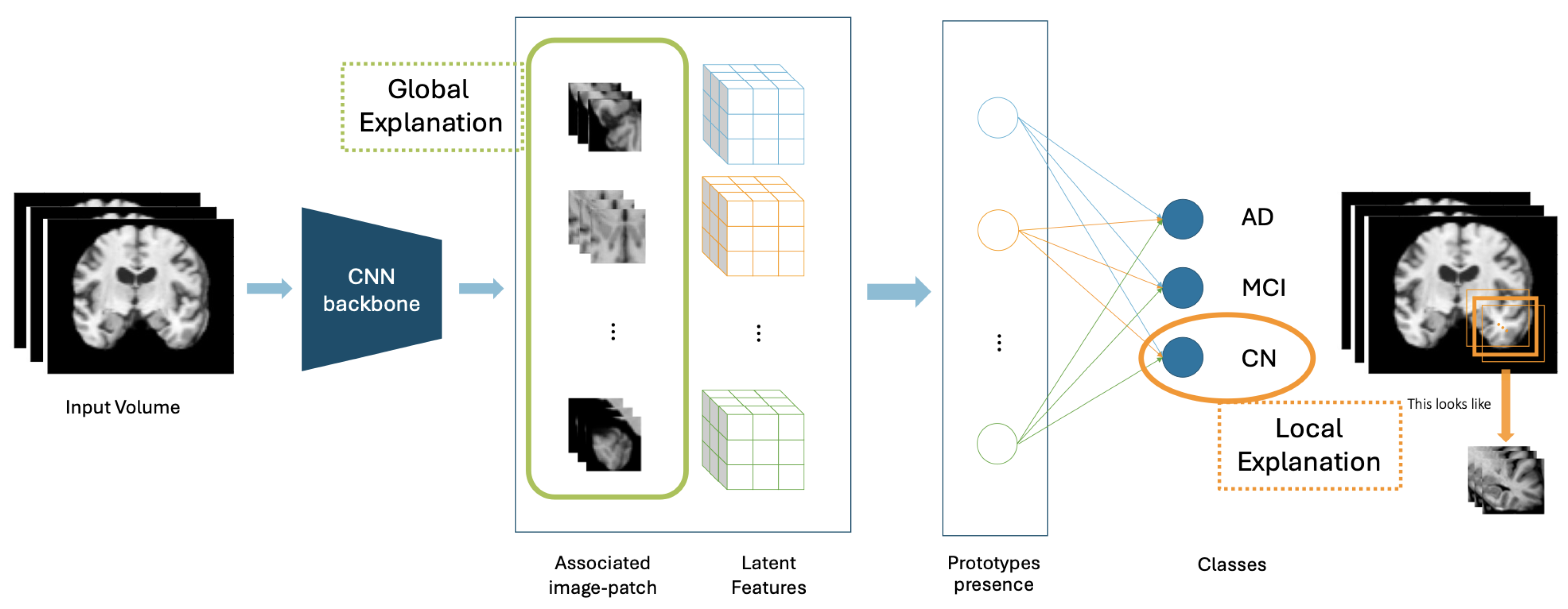
Figure 3.
ProtoPNet architecture

Figure 4.
Prototypical part visualization in a Normal vs. Pneumonia classification task for a Normal test image.
Figure 4.
Prototypical part visualization in a Normal vs. Pneumonia classification task for a Normal test image.
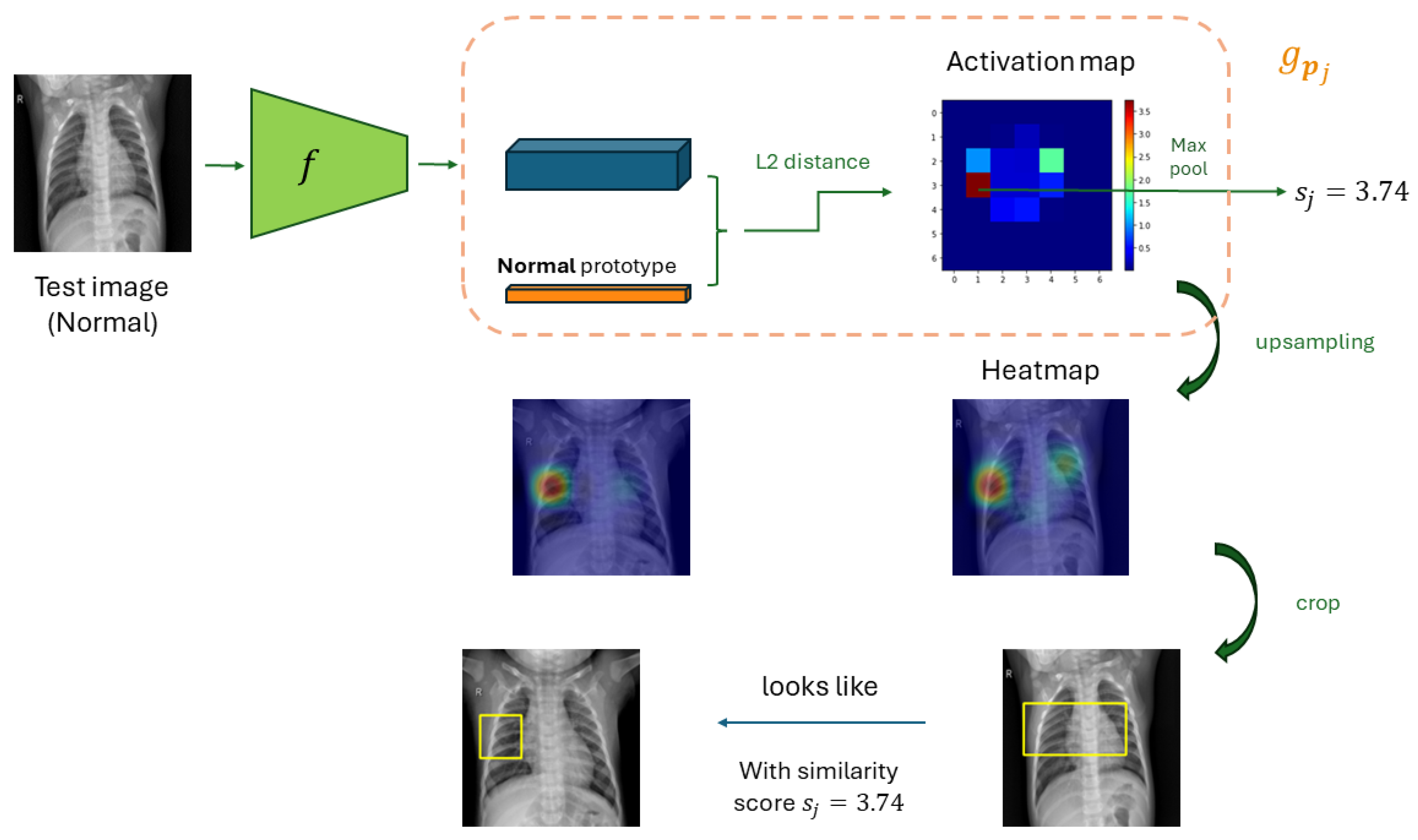
Table 2.
Conceptual Properties (Co-12 Properties) to quantitatively assess quality of Part Prototypes Network, extracted from Nauta et al. [12]
Table 2.
Conceptual Properties (Co-12 Properties) to quantitatively assess quality of Part Prototypes Network, extracted from Nauta et al. [12]
| Co-12 Property | Description |
|---|---|
| Content | |
| Correctness: | Since PP models are interpretable by design, the generation of the explanations is made together with the prediction and the reasoning process is correctly represented by design. By the way, the faithfulness of the prototype visualization (from the latent representation to the input image patches), originally performed by performing a bicubic upsampling, is not guaranteed by design and should be evaluated. |
| Completeness: | The relation between prototypes and classes is transparently shown, so the output-completeness is fulfilled by design, but the computation performed by the CNN backbone is not taken into consideration. |
| Consistency: | PP models should not have random components in their designs, but nondeterminism may occur from the backbones’ initialisation and random seeds. It might be assessed by comparing explanations from models trained with different initializations or with a different shuffling of the training data. |
| Continuity: | Evaluate whether slightly perturbed inputs lead to the same explanation, given that the model makes the same classification. |
| Contrastivity: | The incorporated interpretability of PP models results in a contrastivity incorporated by design, such a different classification corresponds to a different reasoning and hence to a different explanation. This evaluation might also include a target sensitivity analysis, by inspecting where prototypes are detected in the test image. |
| Covariate complexity: | Assess the complexity of the features present in the prototypes with ground truth, such as predefined concepts provided by human judgements (perceived homogeneity) or with object part annotations. |
| Presentation | |
| Compactness: | Evaluate the number of prototypes which constitute the full classification model (global explanation size), in every input image (local explanation sizes), and the redundancy in the information content presented in different prototypes. The size of the explanation should be appropriate to not overwhelm the user. |
| Composition: | Asses how PP can be best presented to the user, and how these prototypes can be best structured and included in the reasoning process by comparing different explanation formats or by asking users about their preferences regarding the presentation and structure of the explanation. |
| Confidence: | Estimate the confidence of the explanation generation method, including measurements such as the prototype similarity scores. |
| User | |
| Context: | Evaluate PP models with application-grounded user studies, similar to evaluation with heatmaps, to understand their needs. |
| Coherence: | Prototypes are often evaluated based on anecdotal evidence, with automated evaluation with an annotated dataset, or with manual evaluation. User studies might include the assessment of satisfaction, preference and trust for part-prototypes. |
| Controllability: | Ability to directly manipulate the explanation and the model’s reasoning e.g., enable users to suppress or modify learned prototypes, eventually with the aid of a graphical user interface. |
Disclaimer/Publisher’s Note: The statements, opinions and data contained in all publications are solely those of the individual author(s) and contributor(s) and not of MDPI and/or the editor(s). MDPI and/or the editor(s) disclaim responsibility for any injury to people or property resulting from any ideas, methods, instructions or products referred to in the content. |
© 2024 by the authors. Licensee MDPI, Basel, Switzerland. This article is an open access article distributed under the terms and conditions of the Creative Commons Attribution (CC BY) license (http://creativecommons.org/licenses/by/4.0/).
Copyright: This open access article is published under a Creative Commons CC BY 4.0 license, which permit the free download, distribution, and reuse, provided that the author and preprint are cited in any reuse.


