Submitted:
09 September 2024
Posted:
09 September 2024
You are already at the latest version
Abstract
Acoustic emissions (AE) are produced by elastic waves generated by damage in solid materials. AE sensors have been widely used in several fields as a promising tool to analyze damage mechanisms such as cracking, dislocation movement, etc. However, accurately determining the location of damage in solids in a non-destructive manner is still challenging. In this paper, we propose a crack wave arrival time determination algorithm that can identify crack waves with low SNR(signal-to-noise ratios) generated in rocks. The basic idea comes from that the variances of the crack wave and noise have different characteristics depending on the size of the moving window. The results can be used to accurately determine the crack source location. The source location is determined by observing where the variance in the crack wave velocities of the true and imaginary crack location reach a minimum. By performing a pencil lead break test using rock samples, it was confirmed that the proposed method could successfully find wave arrival time and crack localization. The results using the proposed algorithm to detect crack wave source localization suggest use for evaluating and real-time monitoring of damage in tunnels or other underground facilities.
Keywords:
Acoustic emission
; variance
; source localization
; crack wave
; time of arrival difference
1. Introduction
A semi-permanent underground high level waste disposal repository can be highly stressed by the high temperature of the used nuclear fuel, underground water, and deep geological conditions [1]. Under such conditions, it is very important to maintain real-time monitoring of the repository’s long-term integrity and evaluate the degree of structural damage to ensure the safety of the disposal system.
To evaluate degree of damage, the most important task is the accurate estimation of crack locations. Time-of-arrival-differences (TOAD) of the crack waves must be accurately measured to precisely calculate crack locations.
Acoustic emission sensors are used to measure crack waves. Recently, the acoustic emission (AE) technique has been widely used for the real-time structural health monitoring of a structure [2,3]. AE has been widely used to evaluate the damage mechanisms of various structures because it is closely related to crack initiation and growth in materials.[4].
A large number of discontinuities formed by blasting and excavation exist around a radioactive waste repository. These discontinuities are the main causes of scattering and dispersion of elastic waves, and interference from reflected waves. In such conditions, the crack wave becomes undetectable because of the noise signal. For this reason, to calculate the exact location of cracks, a method is needed to isolate the crack wave from noise signals.
Traditionally, the estimation of source localization is performed through a triangulation method and a circle intersection technique based on TOAD [5,6]. Recently, a method of calculating TOAD using time-frequency analysis has been studied. Representative time-frequency analysis include Short-time Fourier transform (STFT), wavelet transform and Wigner-Ville distribution. [7,8,9,10,11]. In time-frequency domain, the dispersive characteristics of crack wave are well expressed in homogeneous medium such as metals, but there is a disadvantage that dispersive characteristics do not come out well in a non-homogeneous medium such as rock. Thus, many researches are underway to estimate TOAD and crack location in a rock [12,13].
This paper suggests an algorithm for determining TOADs using moving window, and to calculate a crack location from a crack signal with noise in rocks.
2. Basic Idea
Figure 1 shows the crack wave generated from cracks in rocks. The crack wave starts slightly before 1.3 msec, however a noise signal generated from various causes makes it difficult to accurately determine the arrival time of the crack wave. Given the uncertainty in the arrival time of the crack wave, the estimate of the crack localization contains a significant error. For example, an error of 0.1 msec in the arrival time of a crack wave with a velocity of 5,000 m/s may result in errors of 0.5 meters in the crack localization. To better assess the integrity of structures such as tunnels or other underground facilities, a method is needed to reduce the uncertainty in crack wave arrival time detection, and crack localization.
To more accurately detect the crack wave arrival time from monitoring signals, we first investigated the characteristics of the crack wave and noise signals, employing frequency analysis. Figure 2 shows result of frequency analysis (power spectrum) obtained from crack wave signal. The crack signal obtained by AE sensor is non-stationary signal that has narrow frequency range, while the noise is stationary signal that has broad band as shown in Figure 2. A stationary signal has the characteristic that the ensemble mean and variance value does not change regardless of the signal length. Therefore, if the variance of the crack signal in noisy environment is calculated according to the length change of the signal, the variance of the noise does not change, but only the variance of the crack signal changes as explained in Figure 3.
In this paper, we propose a method of estimating the crack wave arrival time using moving window. The TOAD is estimated by calculating the variance of the measured signal mixed with noise applied to moving window of different sizes as shown in Figure 4. The starting point of the crack signal is the point at which the variances of measured signal change as window size changes.
3. Background Theory for Finding TOAD
As mentioned above, the algorithm determines the variance from the window covering a certain range of signals. Then, an identical method is applied with windows of varying sizes. The theoretical formulas for the proposed method in this chapter are as follows.
The windowed signal of a crack signal can be expressed by the following equation:
where,
where, W(t) is the window function, T is the size of the moving window, N is the number of window data, and is the sampling time.
The variance is as follows:
If the windowed signal is substituted for Eq. (2), the variance of windowed signal can be seen as follows:
And Eq. (3) can be written as Eq. (4).
As shown in Figure 1, a crack signal generated in rock can be expressed as the sum of the background noise and the p-wave signal. If the background noise is assumed to be white noise and its mean is zero, then Eq. (4) can be defined as Eq. (5).
As shown in Eq. (5), the noise signal has a constant value, regardless of the size (T) of the window.
To verify the behavior of the p-wave in Eq. (4), the p-wave is considered to be a sine-wave with the frequency , as follows:
If Eq. (6) is substituted into Eq. (4), as follows:
As can be seen from Eq. (7), now that the p-wave is a function of the size of the window, it can be confirmed that the variance varies according to the size of the window.
Therefore, as can be confirmed from Eq. (5) and Eq. (7), even if a p-wave exists in the noise, if the variance is calculated using the proposed method with the moving window, the noise signal does not change, but the variance of the p-wave changes.
The proposed method calculates the variance while changing the size of the window. Here, determining the window size is the most important factor for ascertaining the arrival time of the p-wave. In this chapter, we will describe how to determine the size of the window.
Figure 5 (b) shows the results of the variance with the size of the window when the p-wave is assumed to be a sine-wave. As can be seen from the graph, it can be confirmed that the change in variance is largest within one wavelength of the p-wave. The size of the window has to be determined within a p-wave wavelength, because the proposed method determines the arrival time of the p-wave by observing the change in variance according to the size of the window.
3. Source Localization Algorithm
Figure 6 explains the concept of the source localization method. When a crack signal is produced at its true source, we can observe the signals with different arrival time delays at sensor 1 and sensor 2. The velocities from the image source x to each sensor can be expressed as follows
where is the initial crack time, and are the measured delay times at each sensor. Because the velocity of the P wave is constant regardless of its source location, the velocities calculated at each sensor are equal. In other words, if the image source moves along the x-axis as shown in Figure 6, the true source location is the point at which the velocities calculated at each sensor are equal.
Because the case in Figure 6 is 1-dimensional, the true source location can be estimated with just two velocities. In order to estimate the true location for two or three dimensions, we must use three or more sensors. For example, if the experiment uses N number of sensors, we can calculate the velocity of the P wave by selecting two sensors. Therefore, M number of velocities are drawn from the calculation.
To define where M number of velocities accord with each other, this paper introduces a variance of velocities to calculate the location of the source. The location of an imaginary source where M number of velocity variances become 0 is where M number of velocities accord with each other, which is the location of true source.
In 1-dimension (Figure 6), the variance of velocities from each sensor is
Where
Then substitute formula (8) to formula (10).
In formula (11), when an image source location accords with a true source location () the variance is 0. Thus, the true source location is where the variance of the velocities is minimal.
The general formula to define a crack location in 3-dimensions is
In this formula, , and means velocity from an imaginary source to the Nth sensor.
4. Validation Using an Experiment
To verify the proposed method for estimating the arrival time and location of crack signal, experiment was carried out using 6 AE sensor on the rock specimens. The AE signal was generated using a pencil lead break and the location of source points and sensors is shown in Table 3 and Figure 7.
As shown in Figure 8, the AE signal was measured using AE-300, which is a program developed by Rectuson & Fuji ceramics, and the AE-603 SW-GA sensor, which has a resonance frequency band in the range of 60 kHz ± 20%. The attachment of the sensor significantly affects the accuracy of the results. For this reason the AE sensors were fixed firmly to the surface of the rock using a high-degree vacuum adhesive. The amplitudes of the free amplifier and the main amplifier were amplified to 40 dB and 20 dB, respectively, because the crack initiation signal has a weak amplitude.
Figure 9 shows the AE signals from each AE sensor when the pencil lead break point was (x,y,z)=(125 mm, 0 mm, 50 mm). The AE signals from Ch.3~Ch.6 arrive earlier than the AE signals from Ch.1~Ch.2. This is because the pencil lead break point is farthest from sensor 1 and sensor 2, and between sensor 3 ~ sensor 6 (Figure 7). Similarly, Figure 10 and Figure 11 show the results from each AE sensor when the pencil lead break point was (x,y,z)=(0 mm, 0 mm, 50 mm), and (x,y,z)=(-125 mm, 0 mm, 50 mm).
In Figure 9, Figure 10 and Figure 11, the defined initiating point (arrival time) has a high probability of error depending on the analyzer. As shown in Figure 12, Figure 13 and Figure 14, it is arrival time when the signal variance initiates to vary according to moving window size which was defined as a result of calculation of raw AE signal, with equation (4) (the proposed moving window method). The estimated arrival time delay obtained using the proposed method is presented in Table 4.
Figure 15, Figure 16 and Figure 17 show the estimated source location results derived by the substitution of Table 1 and Table 2 in equation 11 (Table 1: sensor location; Table 2: arrival time delay calculated for each noise source.). Colors represent the variance in AE wave velocity in Figure 15, Figure 16 and Figure 17. The location of the source is where velocity variance is the least. This is because the velocity variance becomes 0 where the scan source accords with the true source. In Table 3, we present the estimated results of the source location obtained using the above method. As shown in Table 3, the maximum error is 1.5 mm, so the proposed algorithm for arrival time delay and location estimation is valid.
The earlier result from the experiment using a rock specimen had a high signal to noise ratio, and could not be used to verify detection capability, the biggest advantage of the proposed method. Instead, the experiment was carried out using artificial noise.
We supposed that the noise was white noise with a variance size of 340. The signal to noise ratios in sensors 1~6 were respectively 0.025, 0.026, 0.015, 0.016, 0.016, 0.012. These values are too low to define the initial point of the crack signal as directly as Figure 18. However, as shown in Figure 19, we defined the initial point of the crack signal using the moving window method, and estimation was possible based on that initial point, as accurately as Figure 20. This means the proposed method is useful even when the signal to noise ratio is low.
5. Verification Test at In-Situ Test
A field demonstration test was carried out in KURT (KAERI Underground Research Tunnel) in KAERI (Korea Atomic Energy Research Institute). (Figure 21)
As shown in Figure 22, the wall of the tunnel consists of rocks and is finished with shotcrete, and the ground is concrete. The entire interior of the real tunnel is concrete; this research experiment was carried out on the ground. There were 8 AE sensors placed in the tunnel, as shown in Figure 23. The distance between sensors was 0.5 m, and they were arranged in two lines. We excited several points (Figure 23(a)) using an impact hammer (Figure 23(b)) because we could not generate real cracks in the ground at several points. Exciting point 2, in particular, was used to investigate whether the sensors could calculate the crack location, even when the excitation occurred at the edge of the AE sensor array.
Figure 24 shows the results of the calculation with the moving window, and the signals from each sensor, when exciting point 1 was excited with an impact hammer. Figure 25 shows the estimated impact location using the calculated time delay from Figure 24. As shown in the result, the estimated location of excitation (-0.267 m, 0.248 m) was highly accurate, considering the true location of excitation (-0.25 m, 0.25 m). Figure 26 and Figure 27 show the estimated impact location results for each impact using the above method (presented in Table 5).
6. Conclusions
Crack signals from rock and concrete structures occur in conjunction with background noise from various causes. As a result, errors occur when estimating the crack location because the crack wave arrival time cannot be accurately determined. In this paper, by analyzing the crack signal and background noise characteristics, we were able to propose a concept of a ‘moving window’ to accurately determine the crack wave arrival time in a noisy environment. Experiments on a rock specimen and tunnel concrete showed that the proposed method is good at estimating crack locations. It is expected that the proposed method can be applied to the ‘Structural health monitoring’ of large structures, to find defects and weakness such as cracks.
Funding
This work was supported by the National Research Foundation of Korea(NRF) grant funded by the Korea Government(Ministry of Science and ICT) (No. RS-2022-00144206)
Acknowledgement
It is vitally important that scientists are able to describe their work simply and concisely to the public, especially in an open-access on-line journal. The simple summary consists of no more than 200 words in one paragraph and contains a clear statement of the problem addressed, the aims and objectives, pertinent results, conclusions from the study and how they will be valuable to society. This should be written for a lay audience, i.e., no technical terms without explanations. No references are cited and no abbreviations. Submissions without a simple summary will be returned directly. Example could be found at http://www.mdpi.com/2076-2615/6/6/40/htm.
References
- Tsang, C. F., Bernier, F. and Davies, C. (2005), “Geohydromechanical processes in the excavation damaged zone in crystalline rock, rock salt, and indurated and plastic calys-in the context of radioactive waste disposal”, Int. J. Rock Mech. Min. Sci., Vol.42, No.1, pp.109-125. [CrossRef]
- IAEA, (2001), “Monitoring of geological repositories for high level radioactive waste”, IAEA-TECDOC-1208, IAEA, Vienna.
- EU (2004), “Thematic network on the role of monitoring in a phased approach to geological disposal of radioactive waste”, Final report to the European Commission Contract FIKW-CT-2001-20130, pp.1-16.
- hardy, H. R. (1994), “Geotechnical field applications of AE/MS techniques at the Pennsylvania state university: a historical review,” NDT&E International, Vol.27, No.4, pp. 191-200. [CrossRef]
- Tsunoda, T., Kato, T., Hirata, K., Sekido, Y., Segawa, M., Ymamtoku, S., Morioka, T., Sano, K. and Tsuneoka, O. (1985), “Studies on the loose part evaluation technique,” Progress Nuclear Energy, Vol.15, pp.569-576. [CrossRef]
- Olma, B. J. (1985), “Source location and mass estimation in loose parts monitoring of LWR’s,” Progress Nuclear Energy, Vol.15, pp.583-593. [CrossRef]
- Ciampa, F. and Meo, M. (2010), “A new algorithm for acoustic emission localization and flexural group velocity determination in anisotropic structures,” Composites Part A: Applied Science and Manufacturing, Vol. 41, No.12, pp.1777-1786. [CrossRef]
- Jeong, H. and Jang, Y.S. (2000), “Fracture source location in thin plates using the wavelet transform of dispersive waves,” IEEE Trans. Ultras. Ferroelectr. Freq. Control, Vol.47, No.3, pp.612-619. [CrossRef]
- Yaghin, M. A. L. and Koohdaragh, M. (2011), “Examining the function of wavelet packet transform(WPT) and continues wavelet transform(CWT) in recognizing the crack specification”, KSCE Journal of Civil Engineering, Vol.15, No.3, pp.497-506. [CrossRef]
- Park, J. H and Kim, Y. H. (2006), “Impact source localization on an elastic plate in a noisy environment,” Measurement Science and Technology, Vol.17, No.10, pp.2757-2766. [CrossRef]
- Li, Y. and Zheng, X. (2007), “Wigner-Ville distribution and its application in seismic attenuation estimation,” Journal of Applied Geophysics, Vol. 30, No.7, pp.245-254. [CrossRef]
- Choi, Y. C. Kim, J. S. and Park, T. J.(2017), “Estimating arrival time of crack wave by using moving window”, Korean Radioactive waste Society Spring Conference, Korea.
- Choi, Y. C. and Park, T. J.(2016), “A method for detecting crack wave arrival time and crack localization in an tunnel by using moving window technique”, Transaction of the Korean Nuclear Society Spring Meeting, Jeju, Korea, May.
Figure 1.
Crack-wave generated in rock. The sampling frequency is 500 kHz and the number of data is 4096. It is difficult to determine the arrival time of the p-wave in the presence of the ambient noise signal.
Figure 1.
Crack-wave generated in rock. The sampling frequency is 500 kHz and the number of data is 4096. It is difficult to determine the arrival time of the p-wave in the presence of the ambient noise signal.

Figure 2.
The frequency analysis results obtained from the Figure 1 signal. (a) Power spectrum for a crack wave, and (b) power spectrum for background noise. In the frequency characteristics we can observe that a crack wave has a narrow band, and the noise has broad ban.
Figure 2.
The frequency analysis results obtained from the Figure 1 signal. (a) Power spectrum for a crack wave, and (b) power spectrum for background noise. In the frequency characteristics we can observe that a crack wave has a narrow band, and the noise has broad ban.
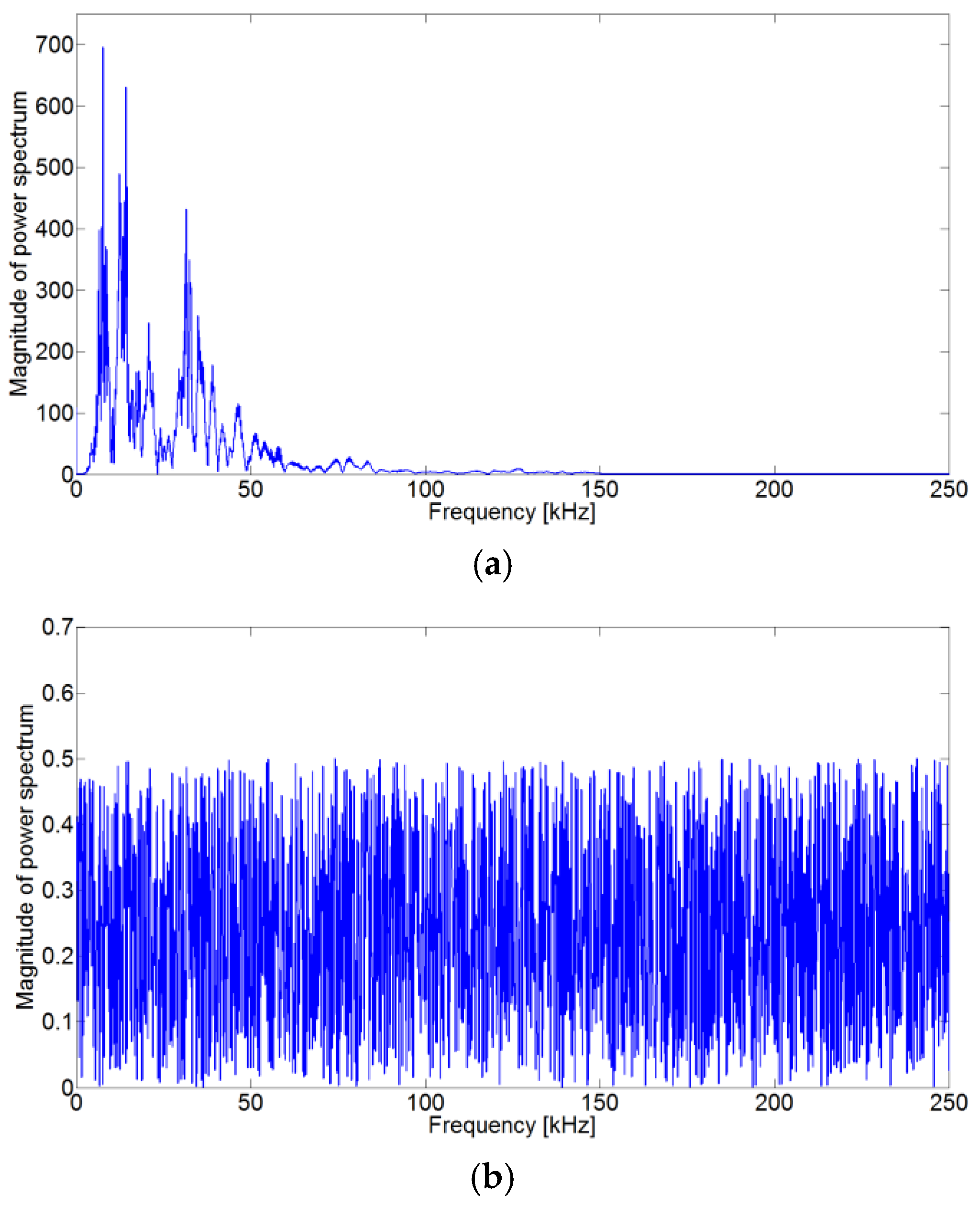
Figure 3.
Signal variance according to window size for (a) noise signal, and (b) crack-wave.
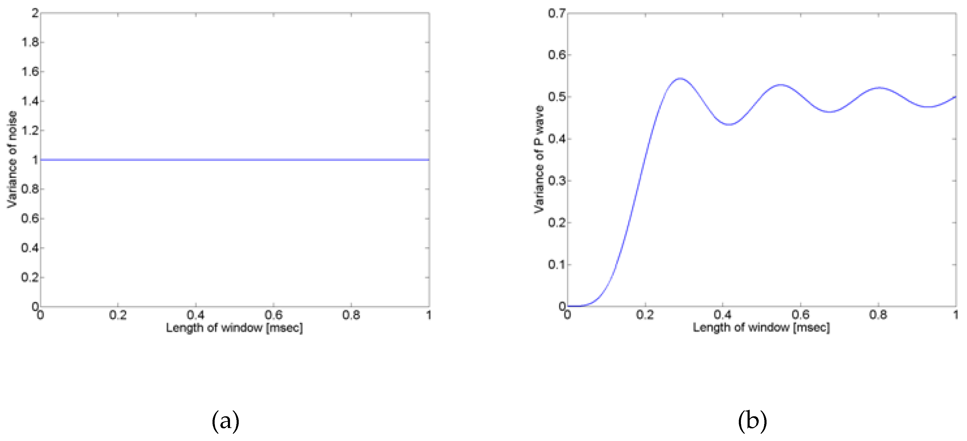
Figure 4.
Proposed algorithm for determining the crack wave arrival time. While calculating the variance during window resizing, the point where the variances are different is the arrival time of the p-wave.
Figure 4.
Proposed algorithm for determining the crack wave arrival time. While calculating the variance during window resizing, the point where the variances are different is the arrival time of the p-wave.
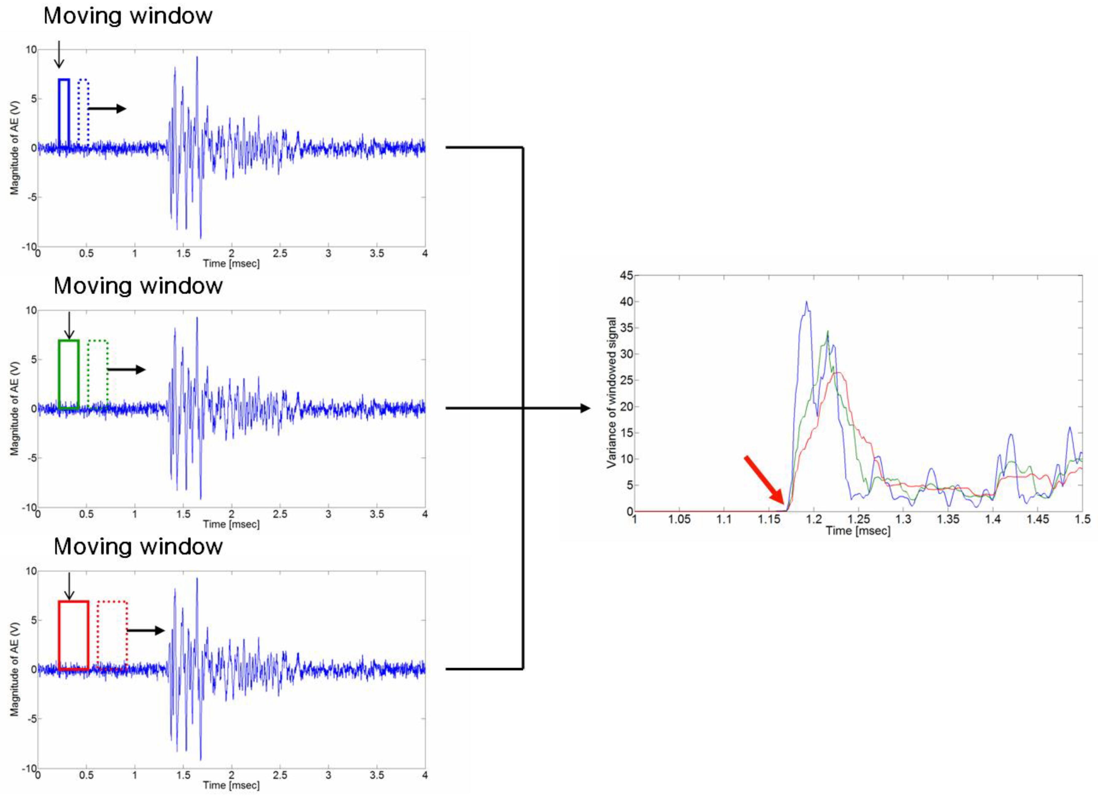
Figure 5.
Results applying the proposed method, assuming the p-wave is a sine-wave. (a) p-wave signal (b) the variance in p-wave using Eq. (4).
Figure 5.
Results applying the proposed method, assuming the p-wave is a sine-wave. (a) p-wave signal (b) the variance in p-wave using Eq. (4).
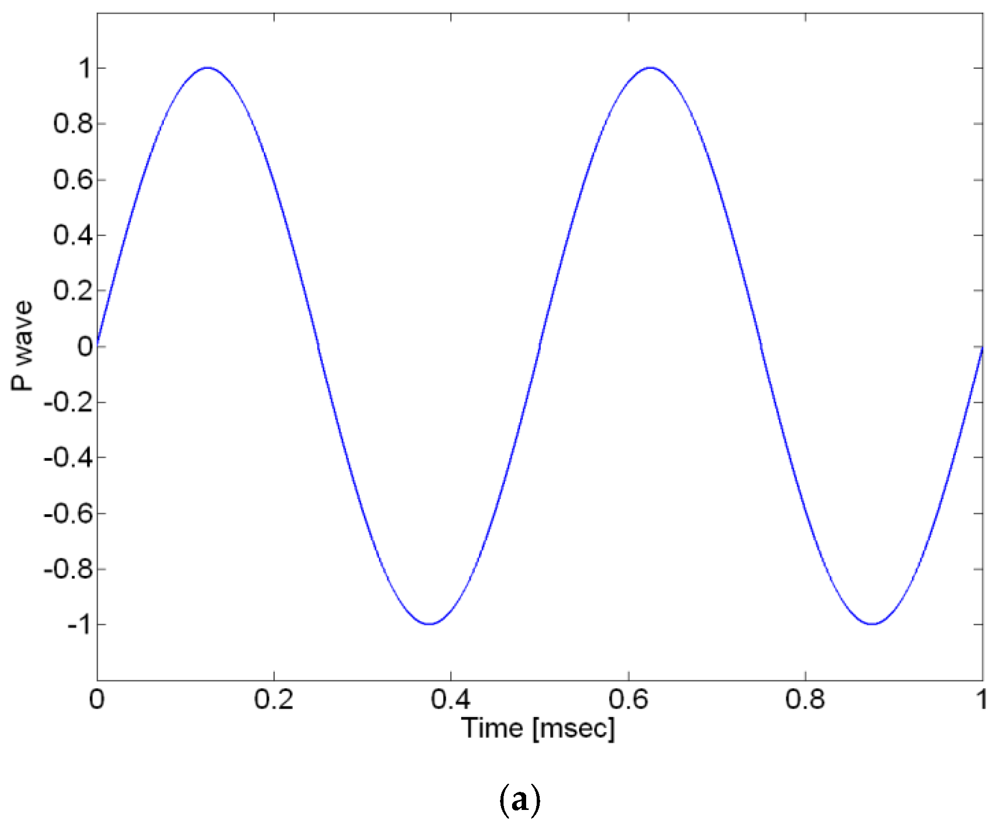
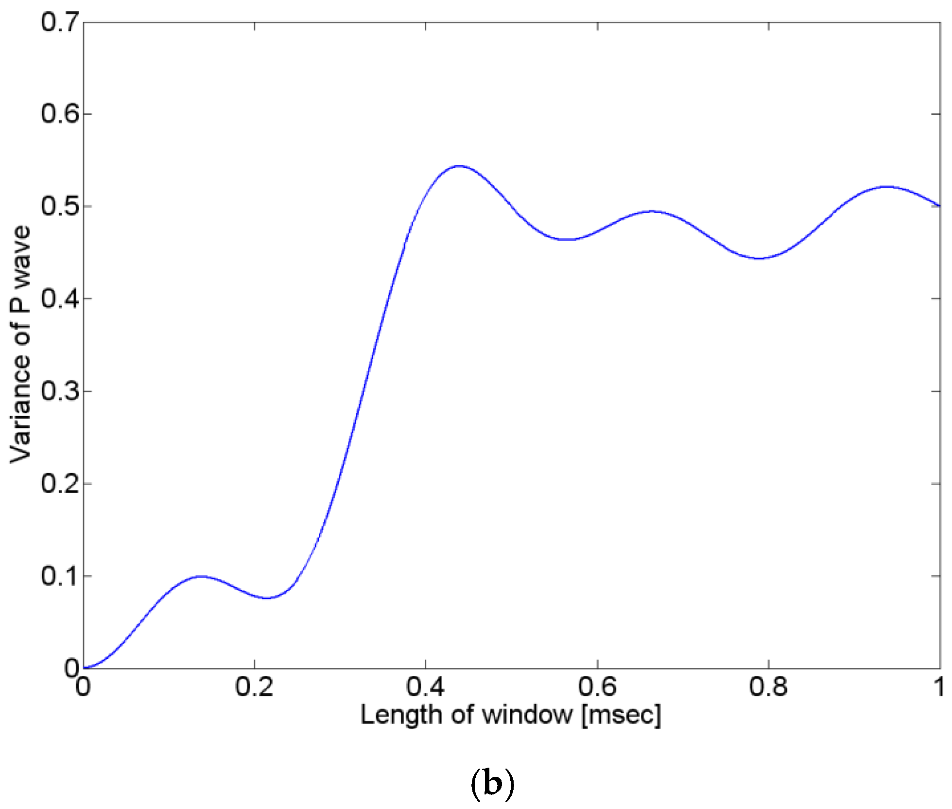
Figure 6.
Concept explanation for source localization.
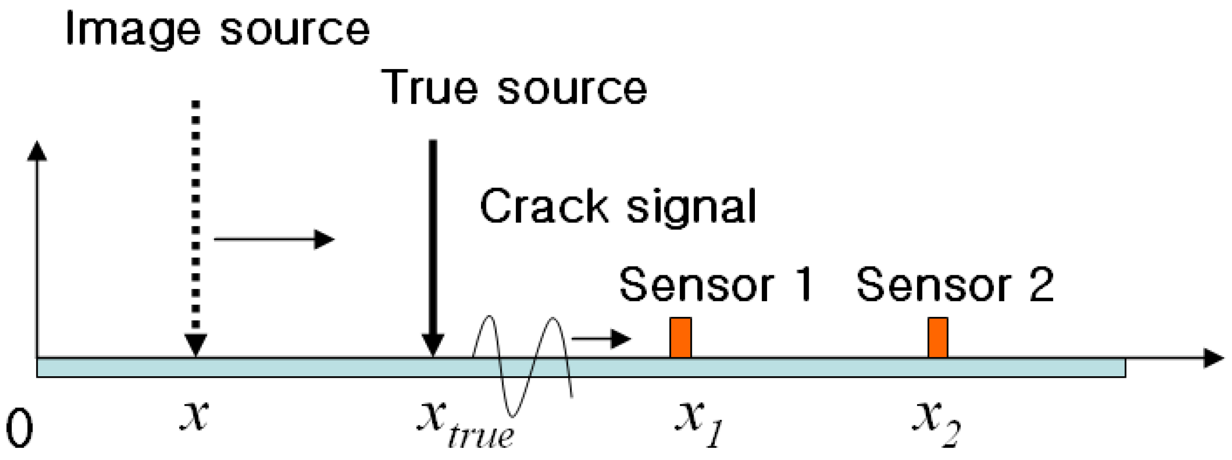
Figure 7.
(a) Location of the AE sensors on the granite rock, and a schematic diagram of the pencil lead break experiment to test the accuracy of the method for source localization. (b) Picture of the experimental setup.
Figure 7.
(a) Location of the AE sensors on the granite rock, and a schematic diagram of the pencil lead break experiment to test the accuracy of the method for source localization. (b) Picture of the experimental setup.
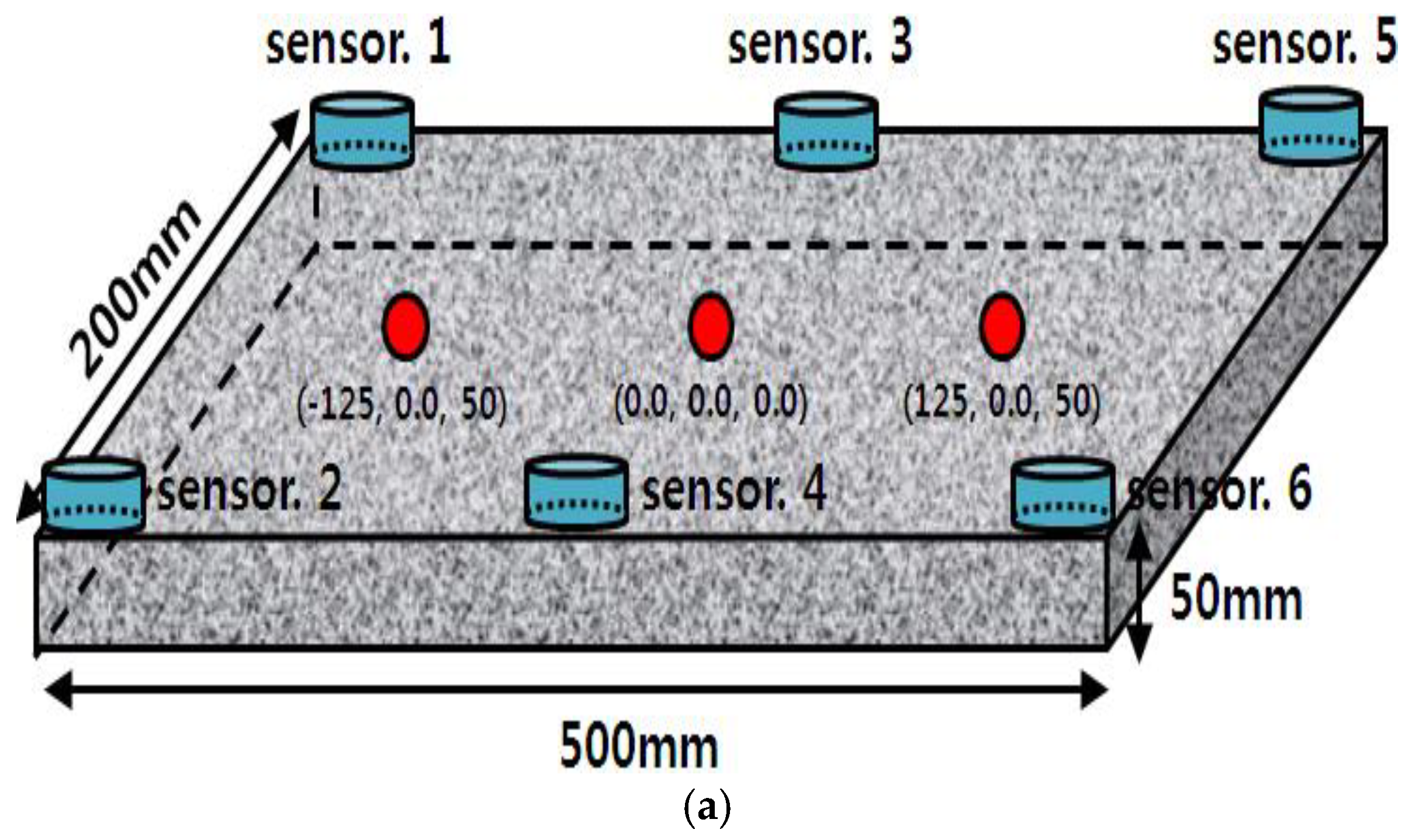
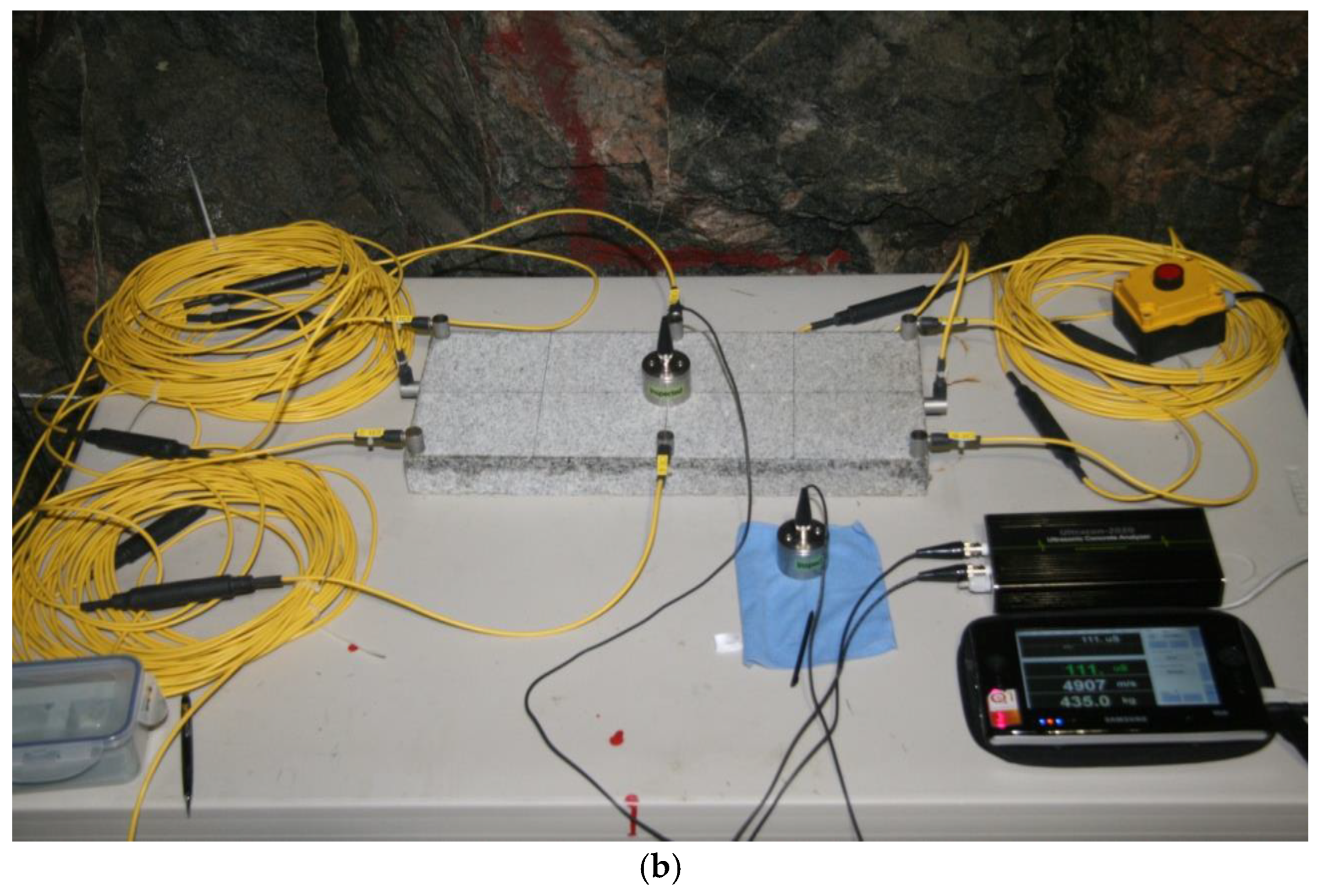
Figure 8.
AE sensors and instruments used in this test. (a) AE-300, (b) AE-603 SW-GA sensor.
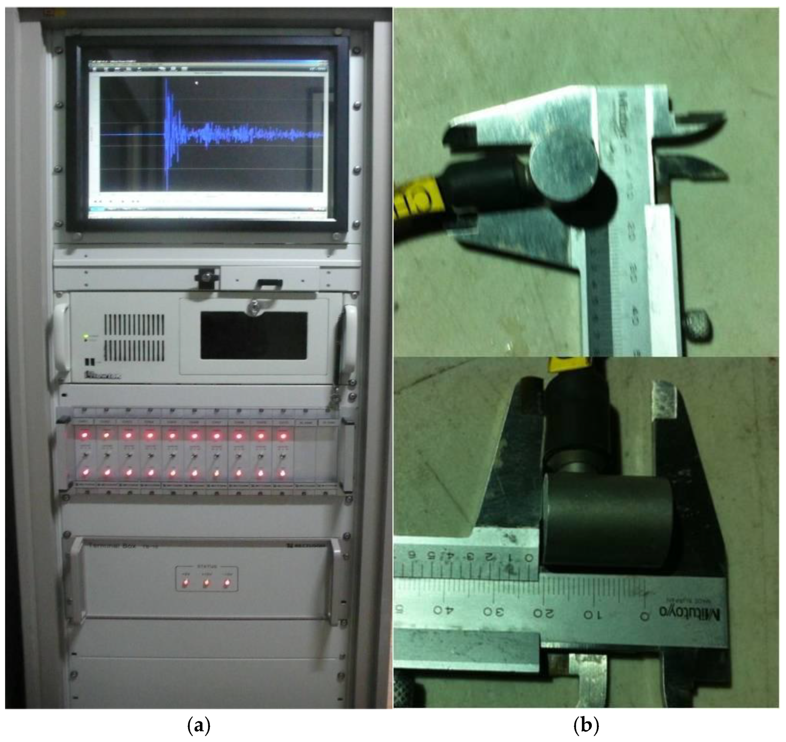
Figure 9.
Measured signals when the pencil lead break test was performed at (125mm, 0.0mm, 50mm).
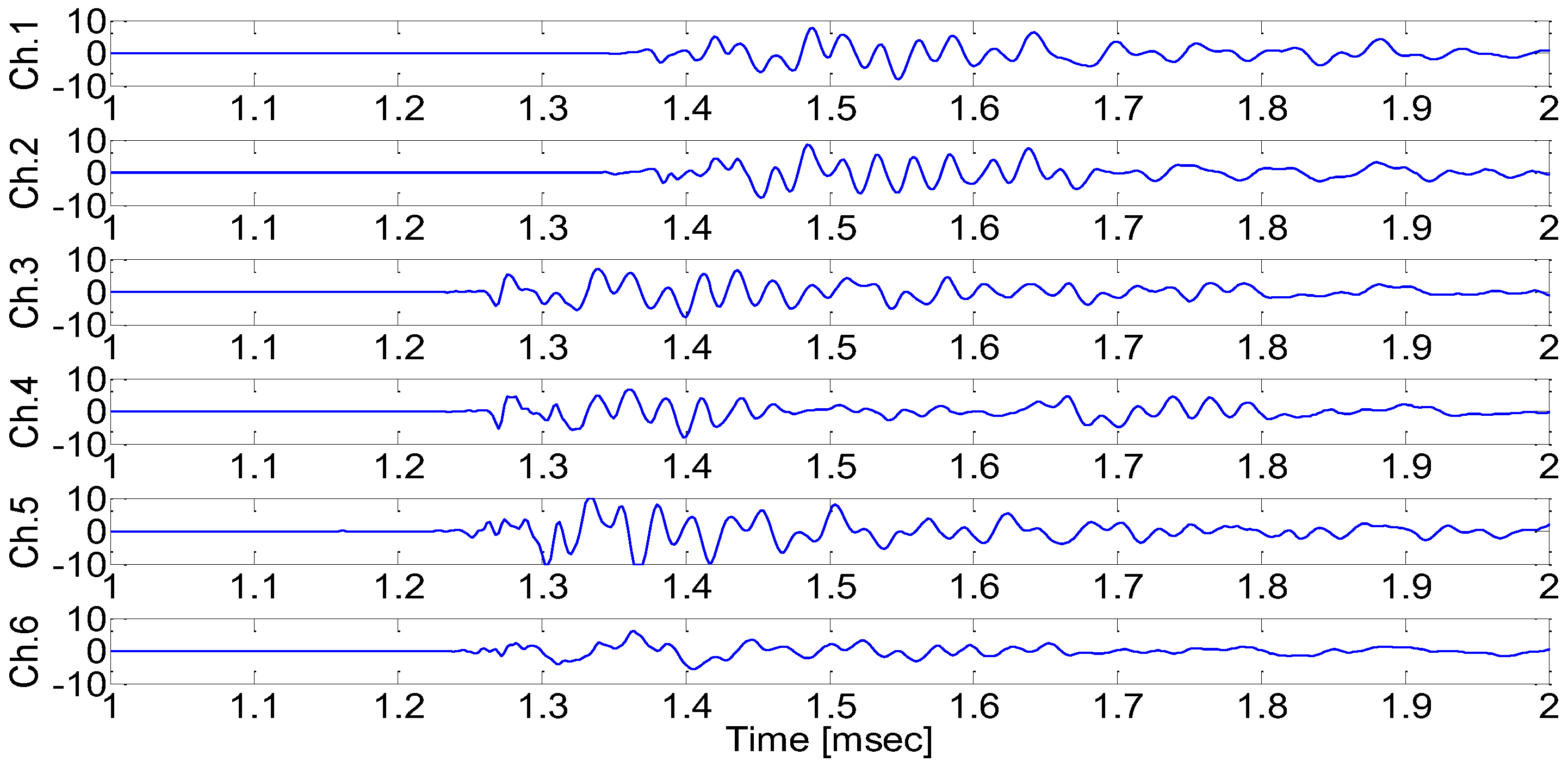
Figure 10.
Measured signals when the pencil lead break test was performed at (0mm, 0 mm, 50mm).
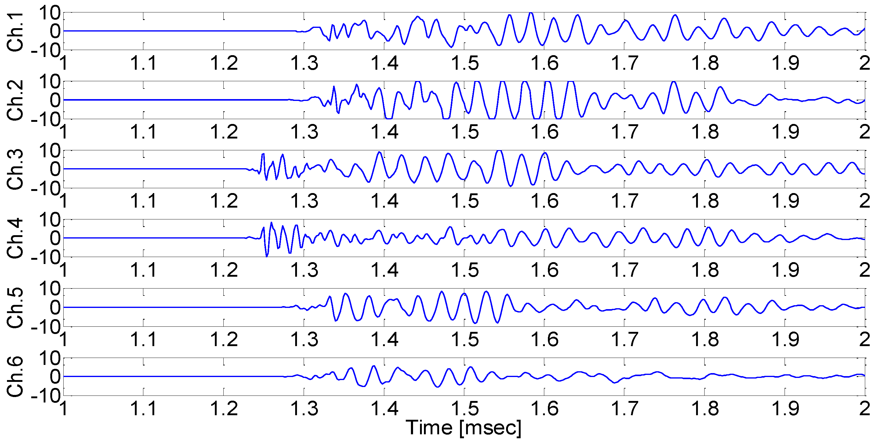
Figure 11.
Measured signals when the pencil lead break test was performed at (-125mm, 0mm, 50mm).
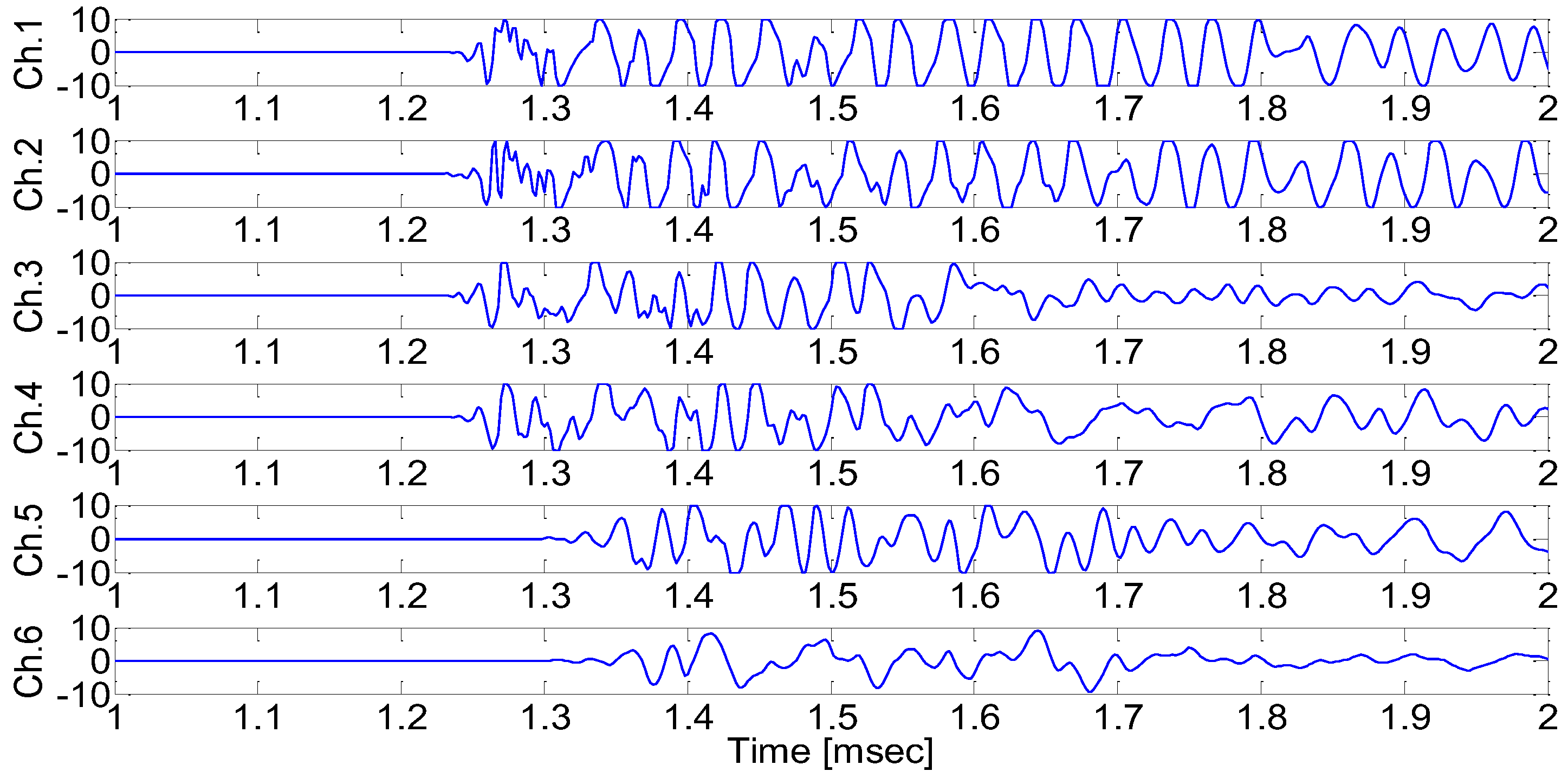
Figure 12.
Experimental results using the proposed moving window method when the pencil lead break test was performed at (125mm, 0.0mm, 50mm).
Figure 12.
Experimental results using the proposed moving window method when the pencil lead break test was performed at (125mm, 0.0mm, 50mm).
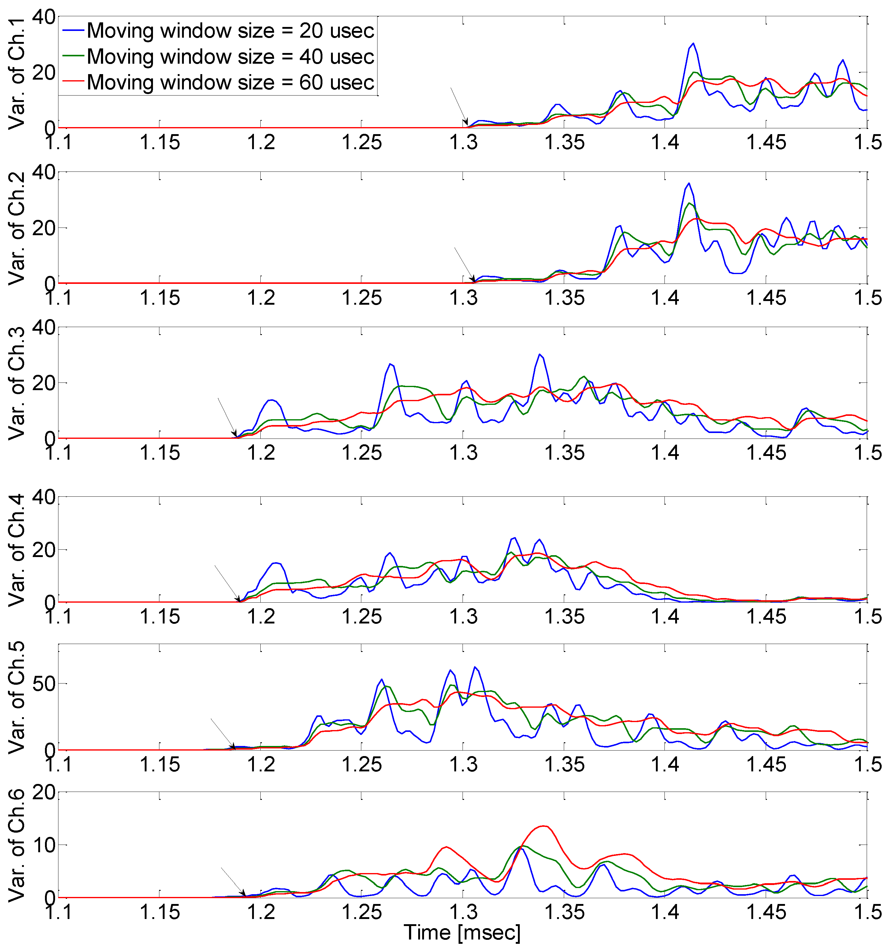
Figure 13.
Experimental results using the proposed moving window method when the pencil lead break test was performed at (0mm, 0 mm, 50mm ).
Figure 13.
Experimental results using the proposed moving window method when the pencil lead break test was performed at (0mm, 0 mm, 50mm ).
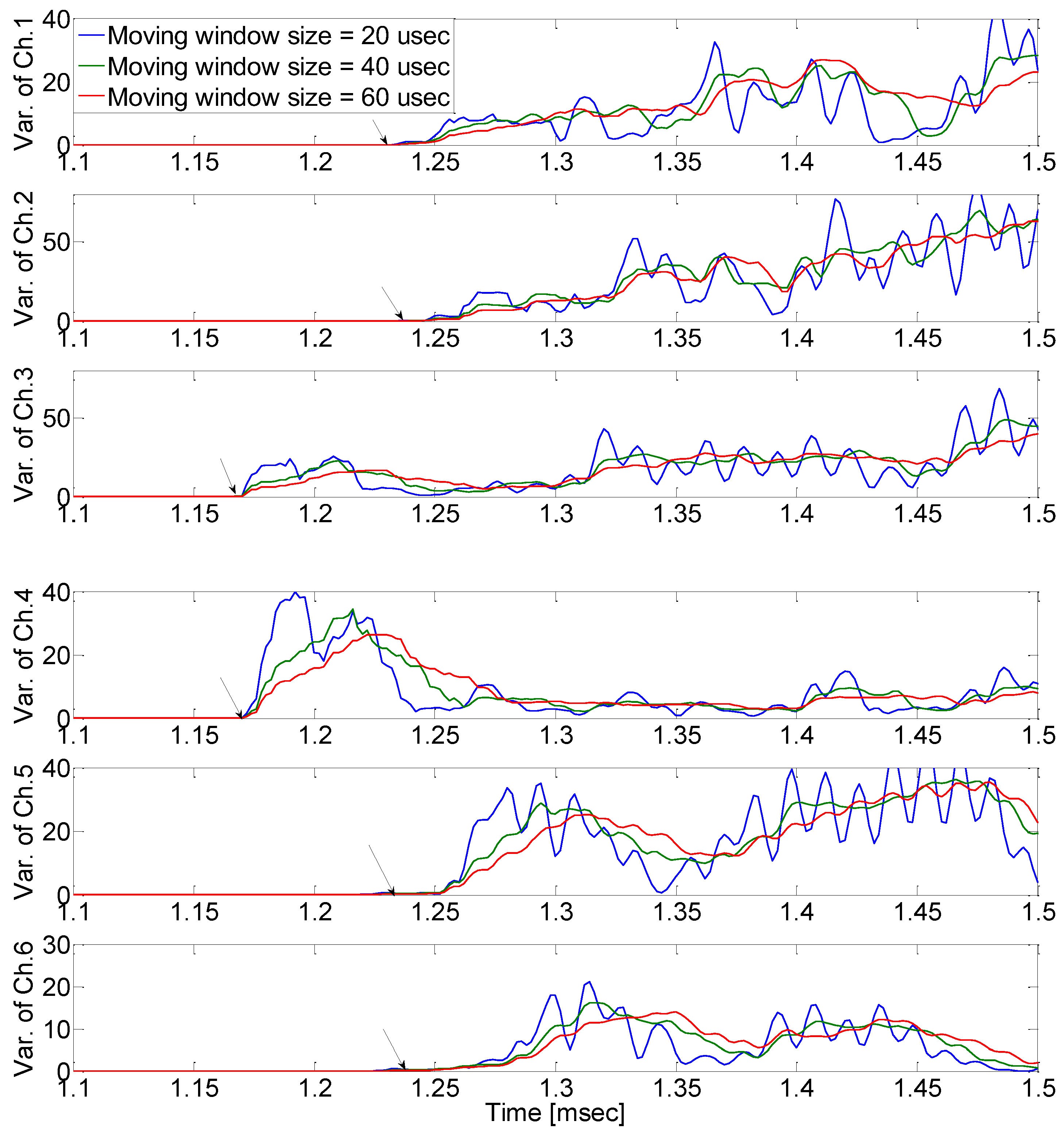
Figure 14.
Experimental results using the proposed moving window method when the pencil lead break test was performed at (-125mm, 0mm, 50mm).
Figure 14.
Experimental results using the proposed moving window method when the pencil lead break test was performed at (-125mm, 0mm, 50mm).
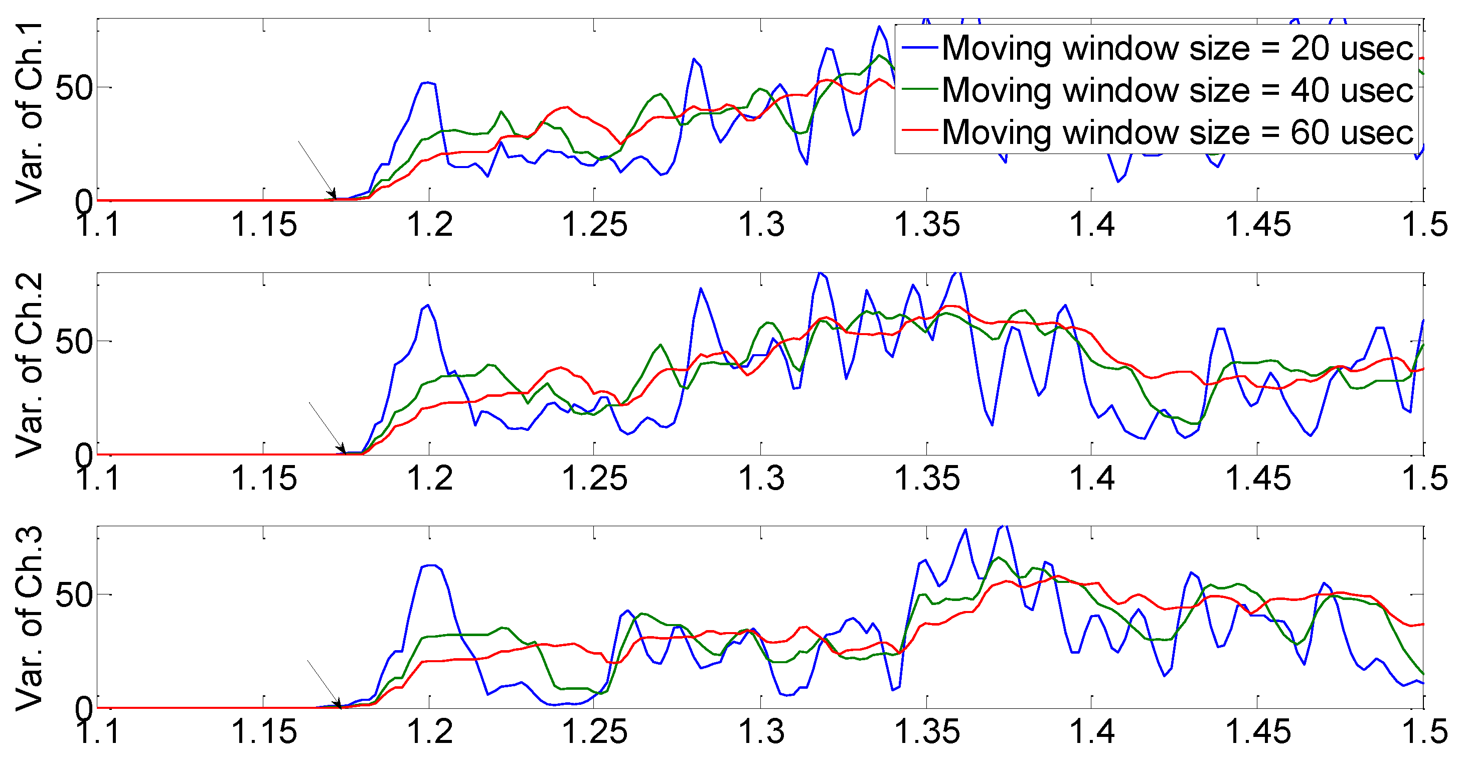
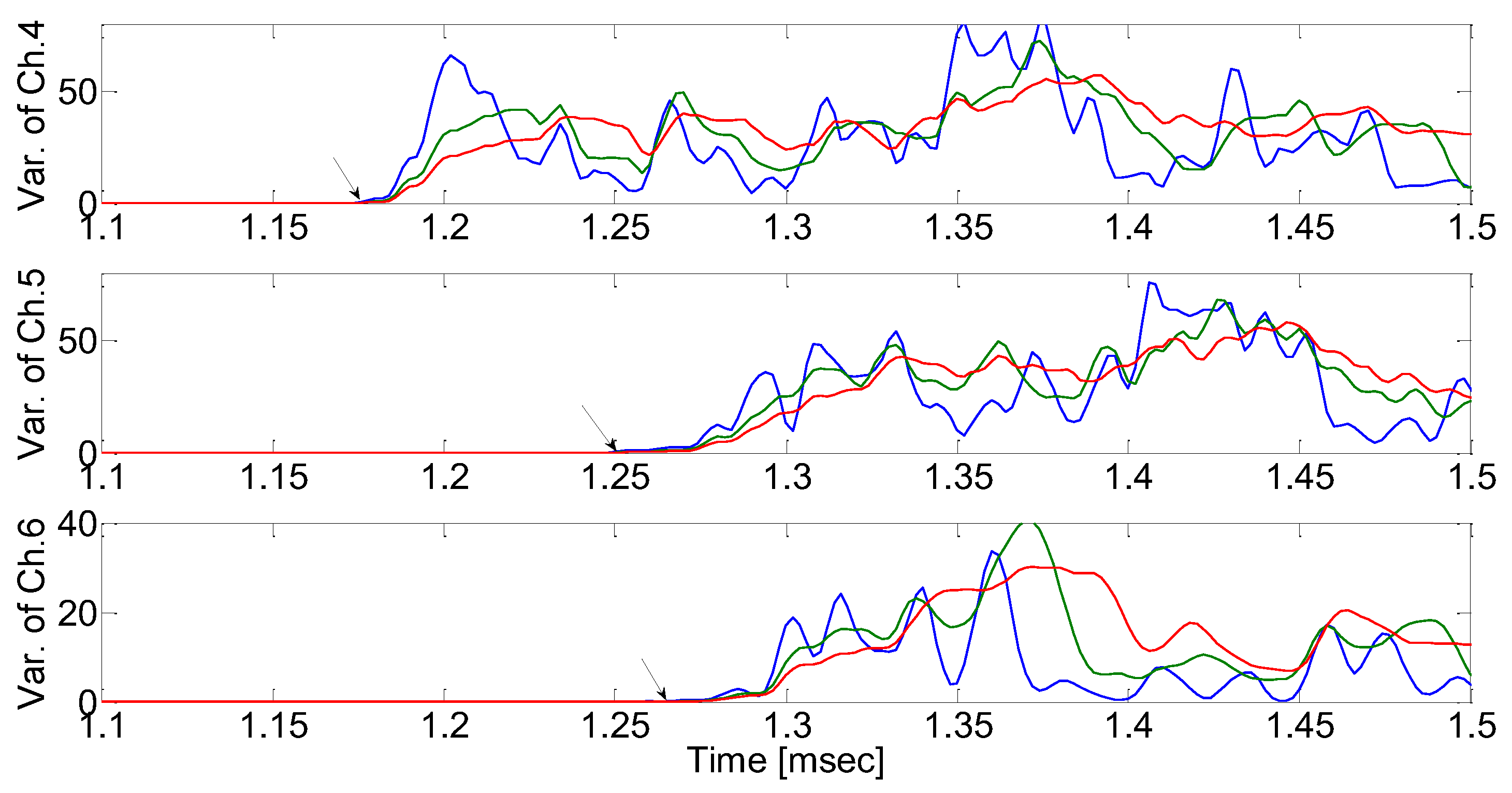
Figure 15.
Source location was estimated by calculating the variance in velocities; the minimum value of variance indicates the source location. The estimated source location was (125.8mm, 2.7mm, 50mm) while the true source location was (125mm, 0mm, 50mm).
Figure 15.
Source location was estimated by calculating the variance in velocities; the minimum value of variance indicates the source location. The estimated source location was (125.8mm, 2.7mm, 50mm) while the true source location was (125mm, 0mm, 50mm).
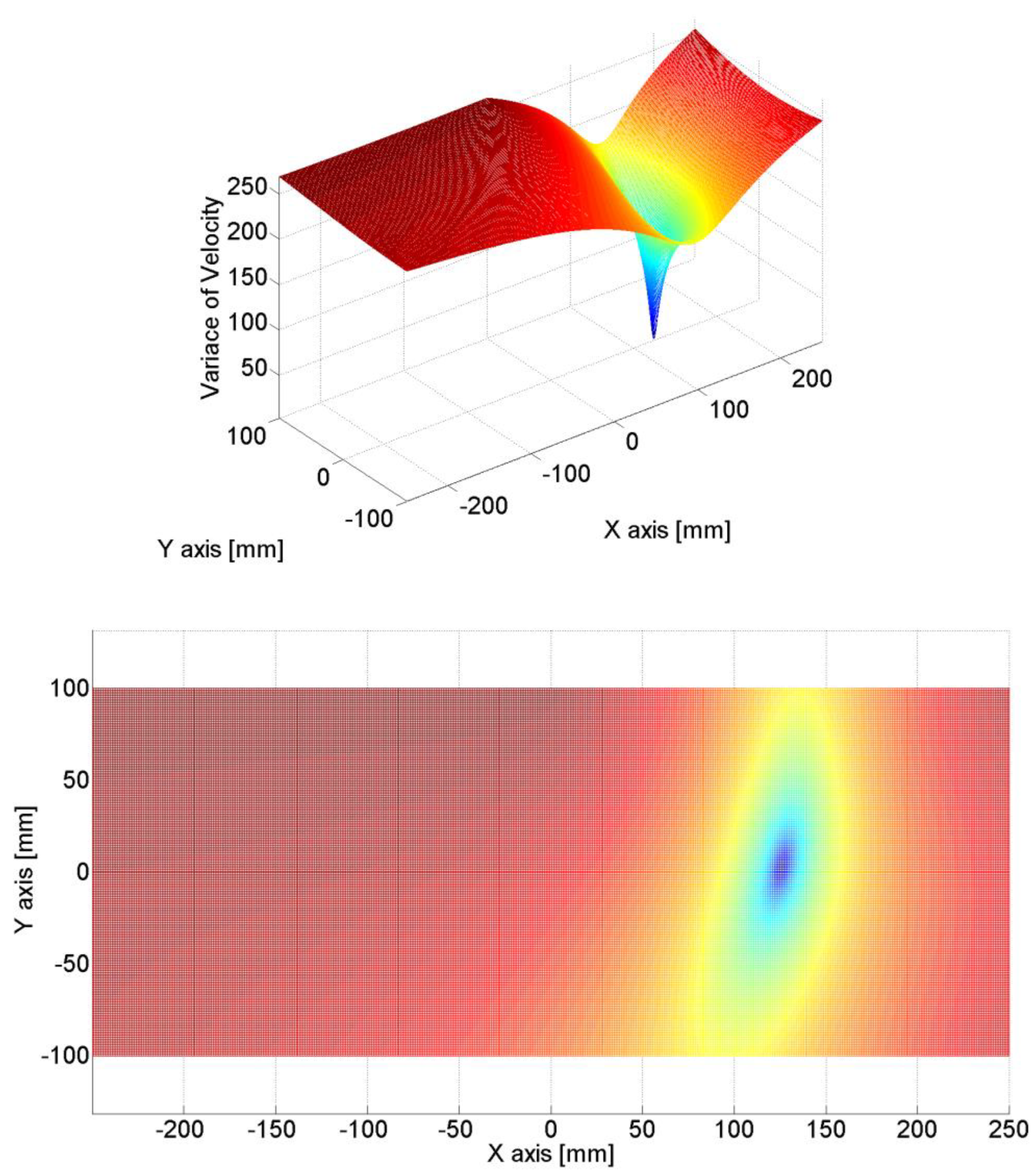
Figure 16.
Source location was estimated by calculating the variance in velocities; the minimum value of variance indicates the source location. The estimated source location was (-0.5mm, 0.5mm, 50mm) while the true source location was (0mm, 0mm, 50mm).
Figure 16.
Source location was estimated by calculating the variance in velocities; the minimum value of variance indicates the source location. The estimated source location was (-0.5mm, 0.5mm, 50mm) while the true source location was (0mm, 0mm, 50mm).
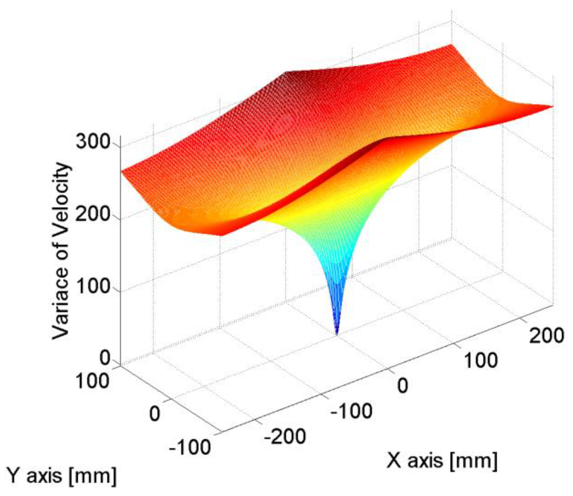
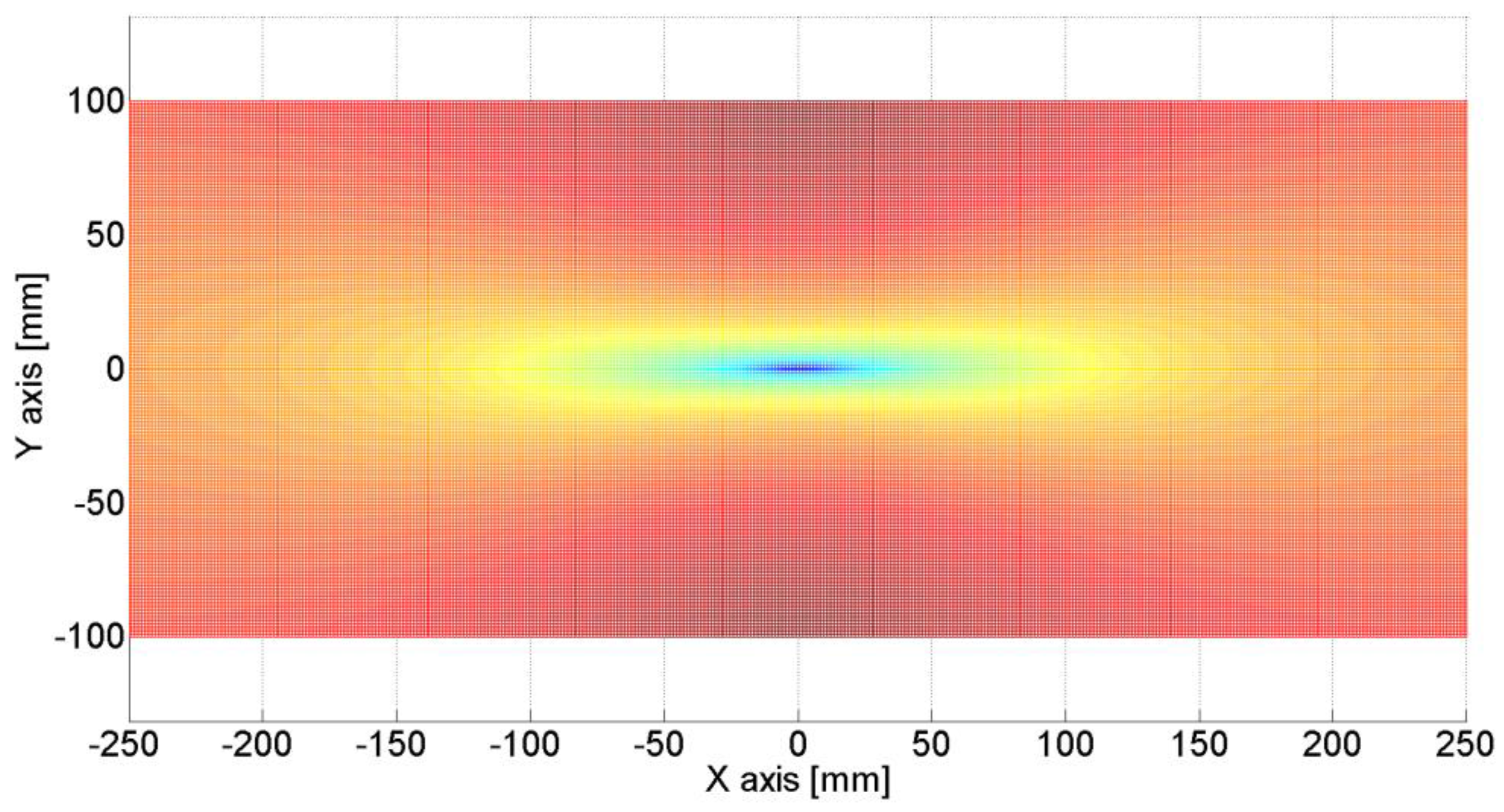
Figure 17.
Source location was estimated by calculating the variance in velocities; the minimum value of variance indicates the source location. The estimated source location was (-124.7mm, 1.5mm, 50mm) while the true source location was (-125mm, 0mm, 50mm).
Figure 17.
Source location was estimated by calculating the variance in velocities; the minimum value of variance indicates the source location. The estimated source location was (-124.7mm, 1.5mm, 50mm) while the true source location was (-125mm, 0mm, 50mm).
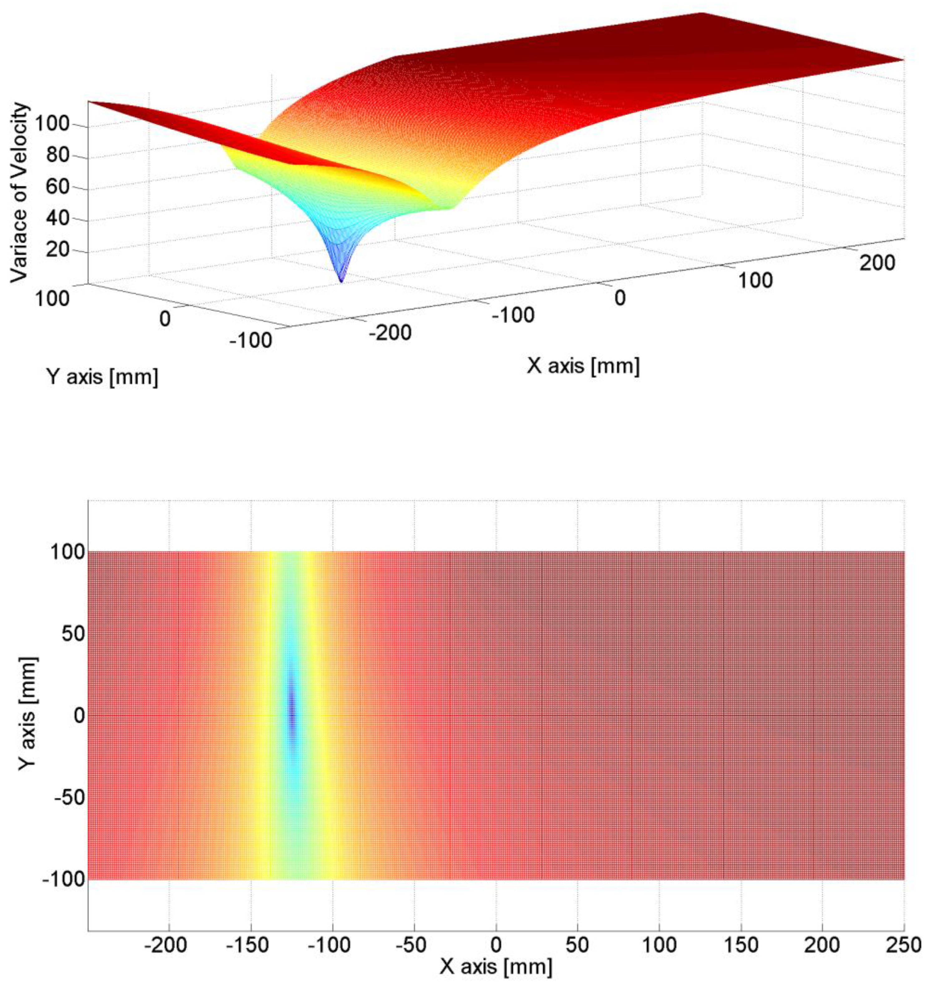
Figure 18.
The signals were a mixture of artificial noise and Figure 11 signals when the pencil lead break test was performed at (-125mm, 0mm, 50mm).
Figure 18.
The signals were a mixture of artificial noise and Figure 11 signals when the pencil lead break test was performed at (-125mm, 0mm, 50mm).
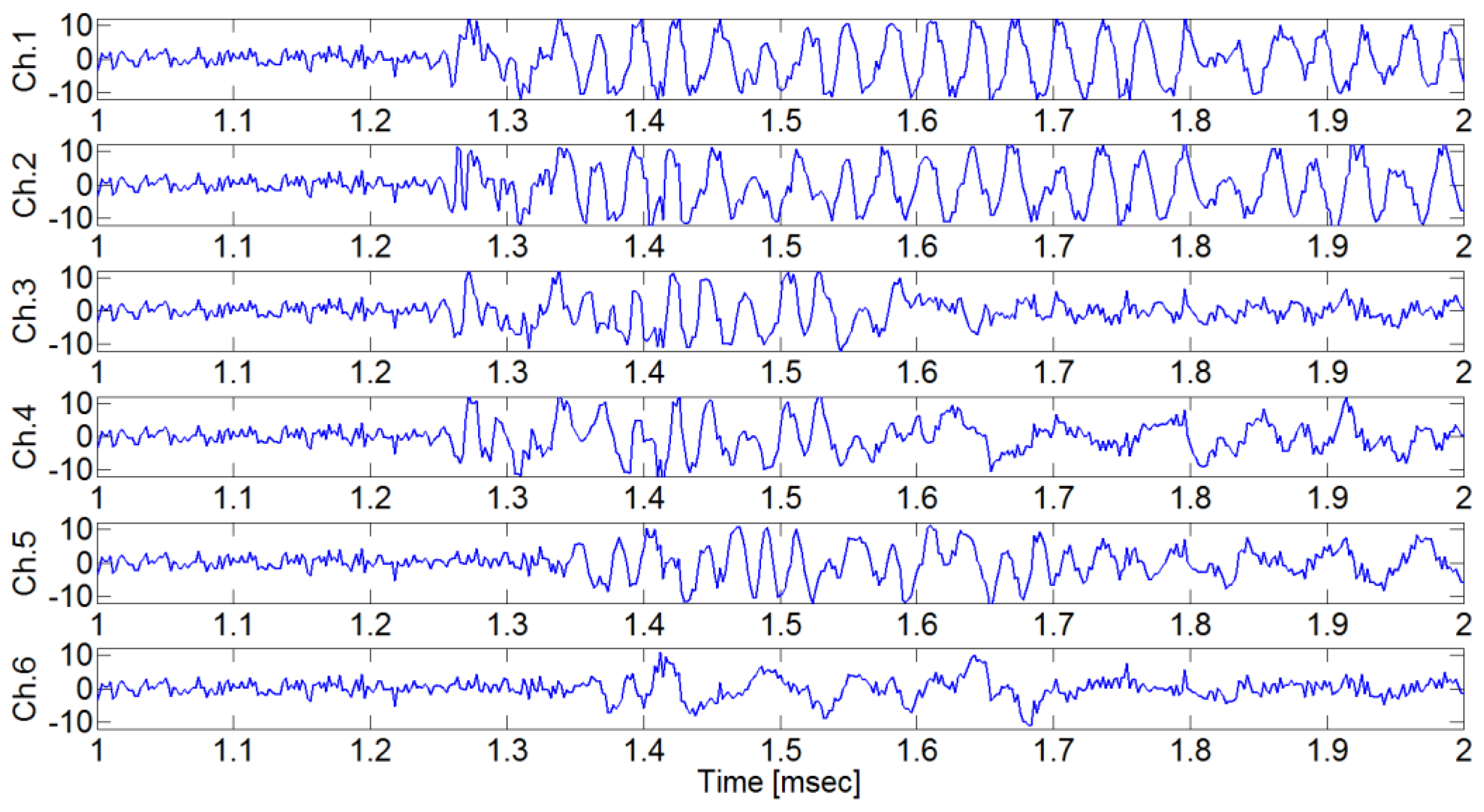
Figure 19.
Experimental results in a noisy environment when the pencil lead break test was performed at (-125mm, 0mm, 50mm).
Figure 19.
Experimental results in a noisy environment when the pencil lead break test was performed at (-125mm, 0mm, 50mm).
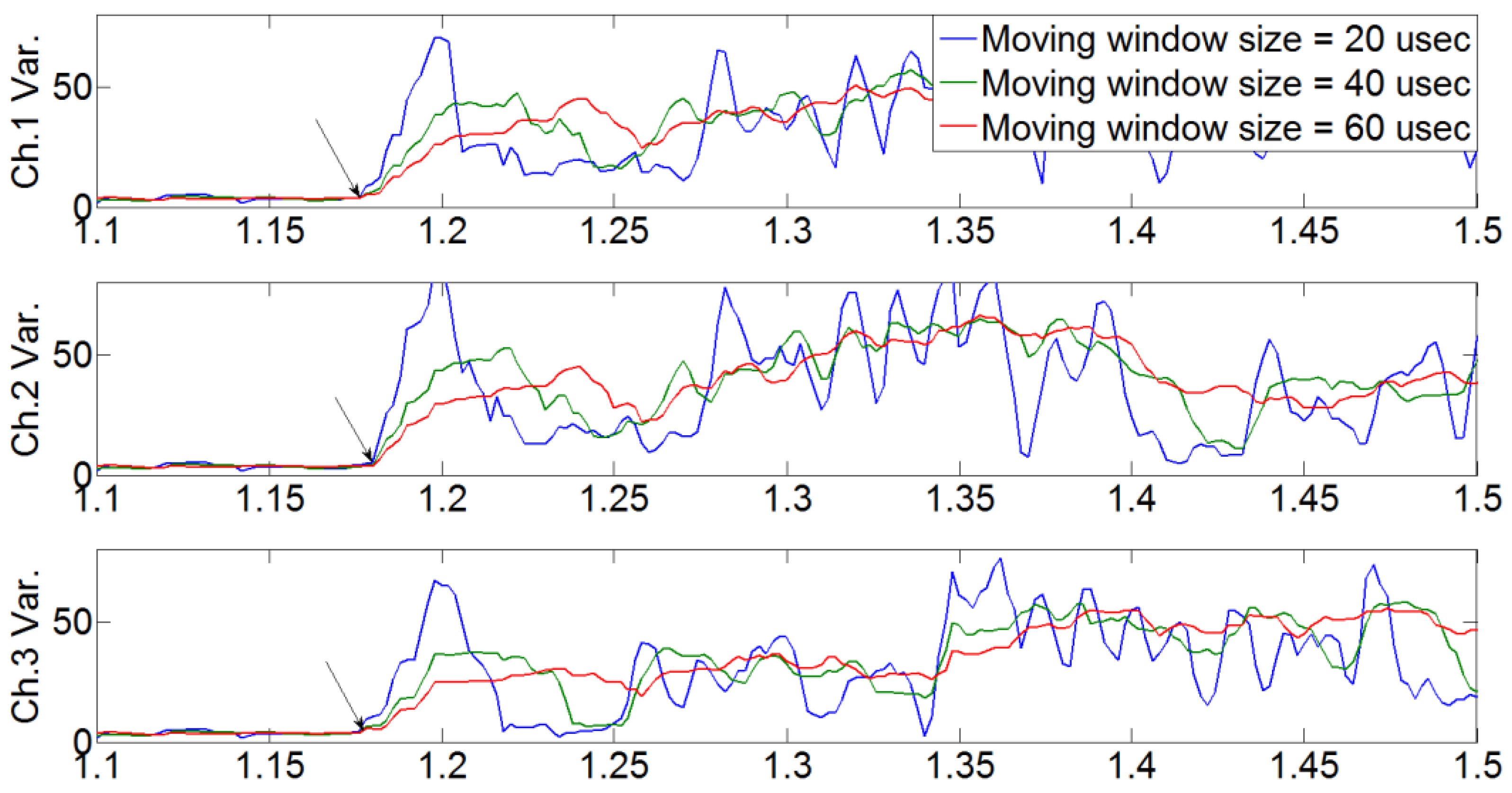
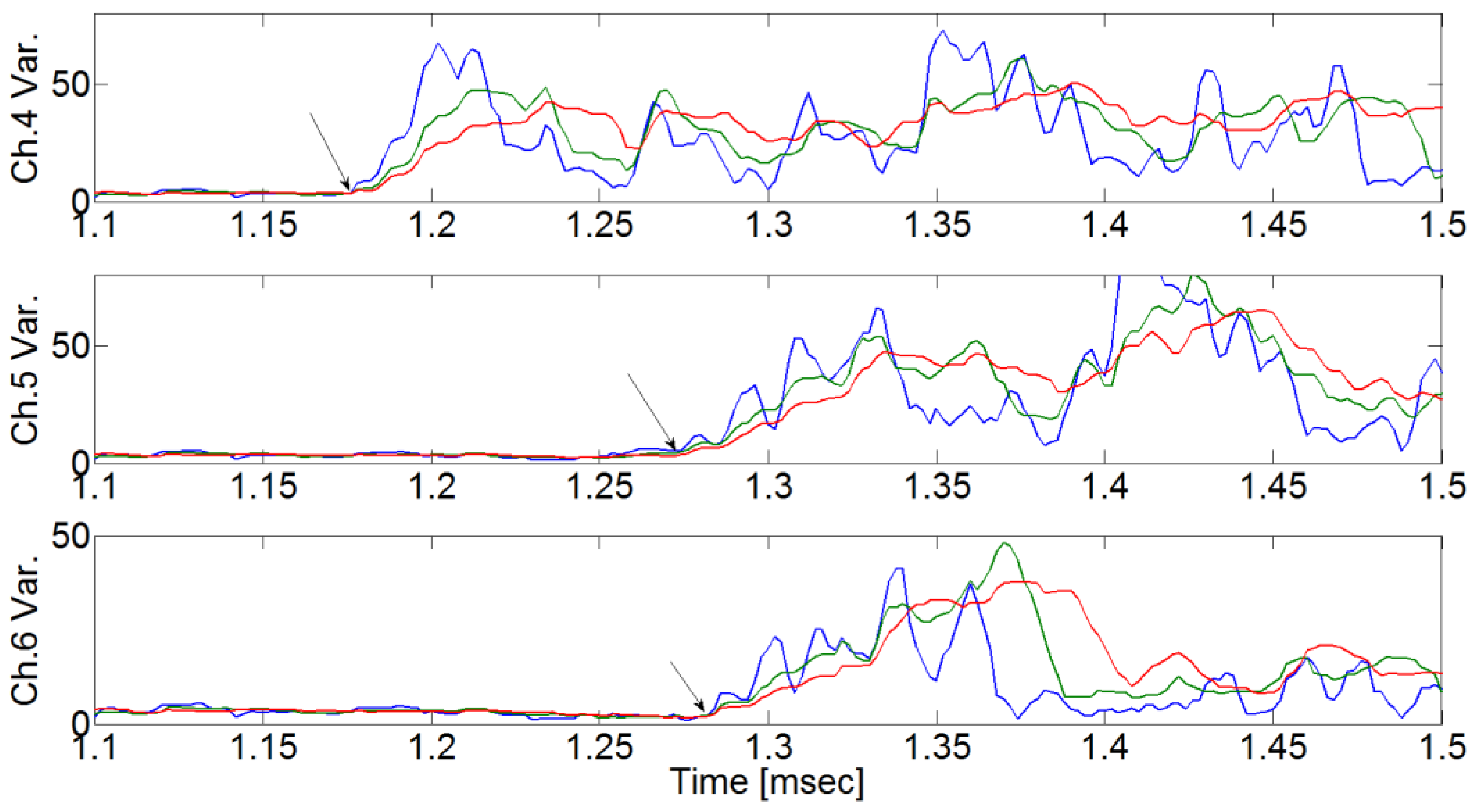
Figure 20.
The source localization result. The estimated source location was (-124.7mm, 0.5mm, 50mm) while the true source location was (-125mm, 0mm, 50mm).
Figure 20.
The source localization result. The estimated source location was (-124.7mm, 0.5mm, 50mm) while the true source location was (-125mm, 0mm, 50mm).
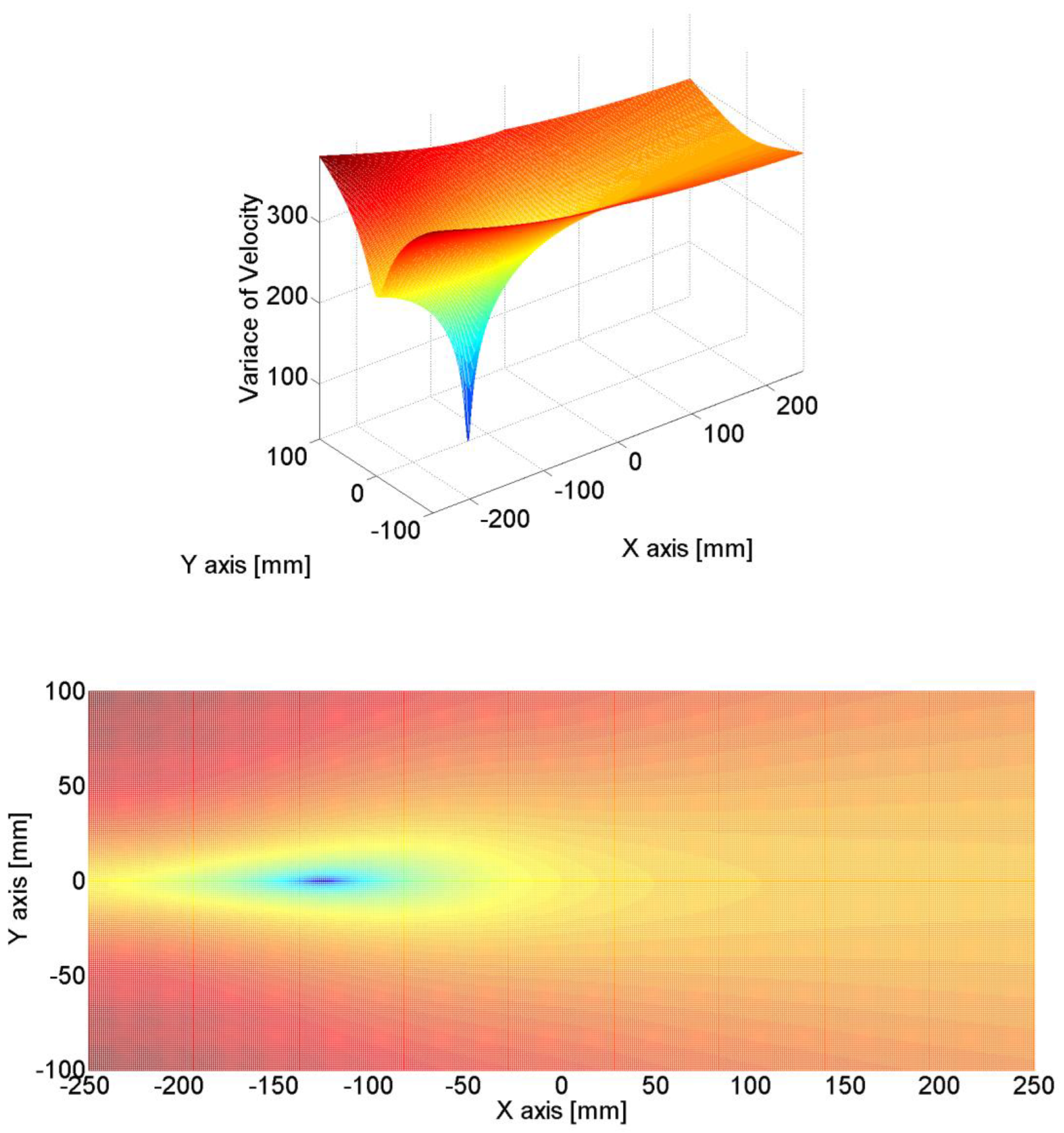
Figure 21.
KURT (Korea Underground Research Tunnel).
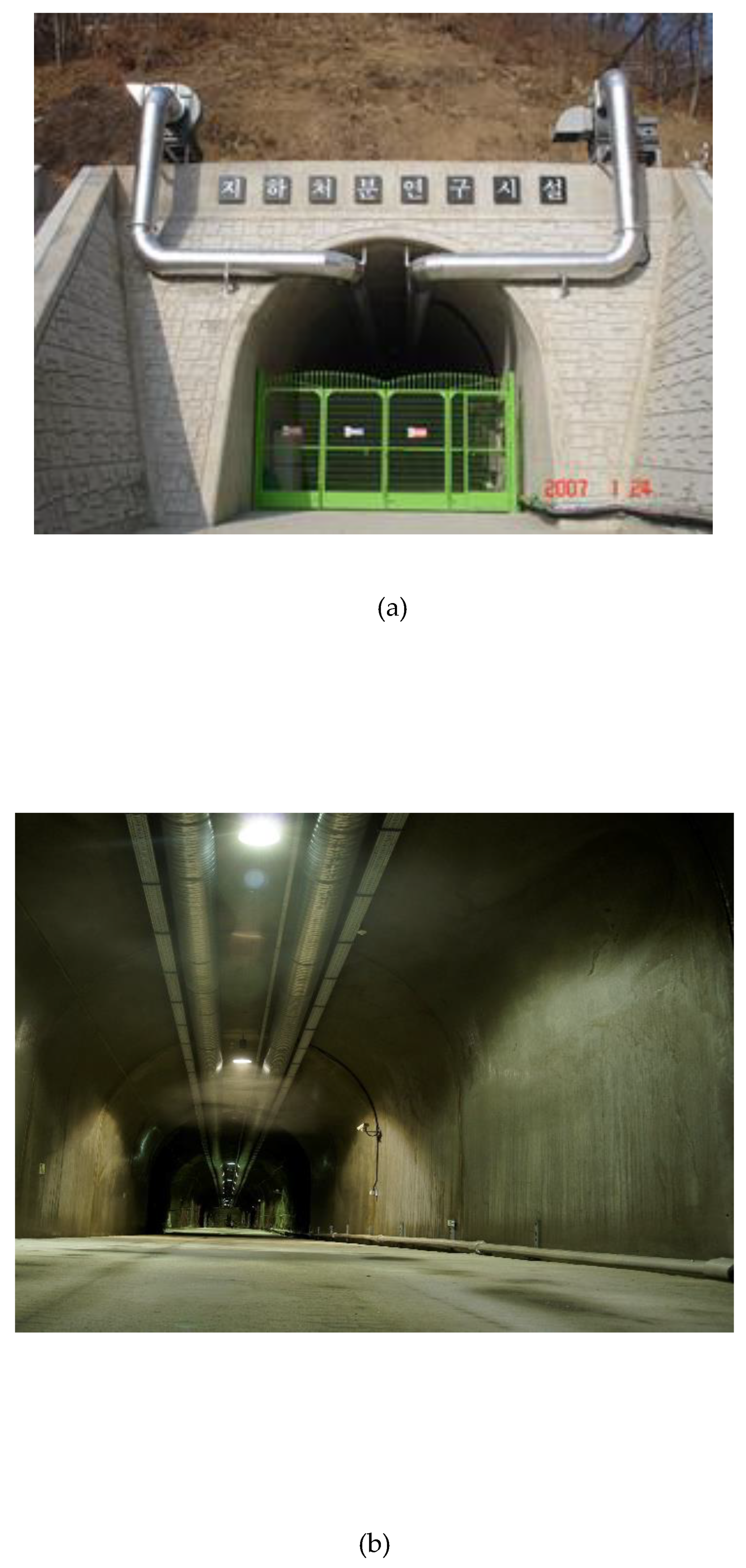
Figure 22.
At the entrance of KURT research module 3.
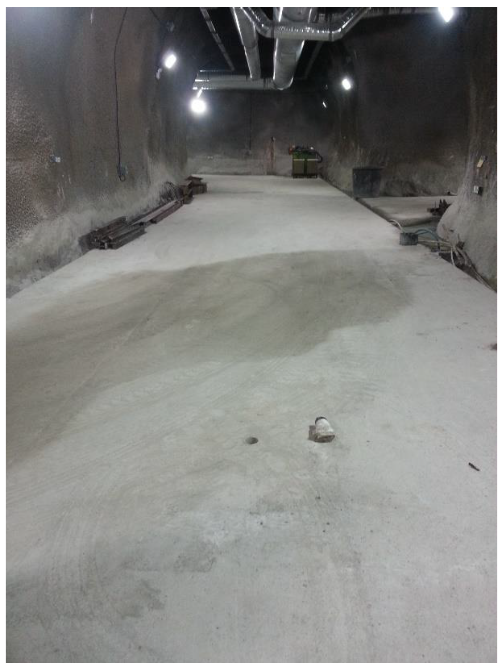
Figure 23.
(a) Location of AE sensors and exciting points on the ground of tunnel and (b) experimental pictures.
Figure 23.
(a) Location of AE sensors and exciting points on the ground of tunnel and (b) experimental pictures.
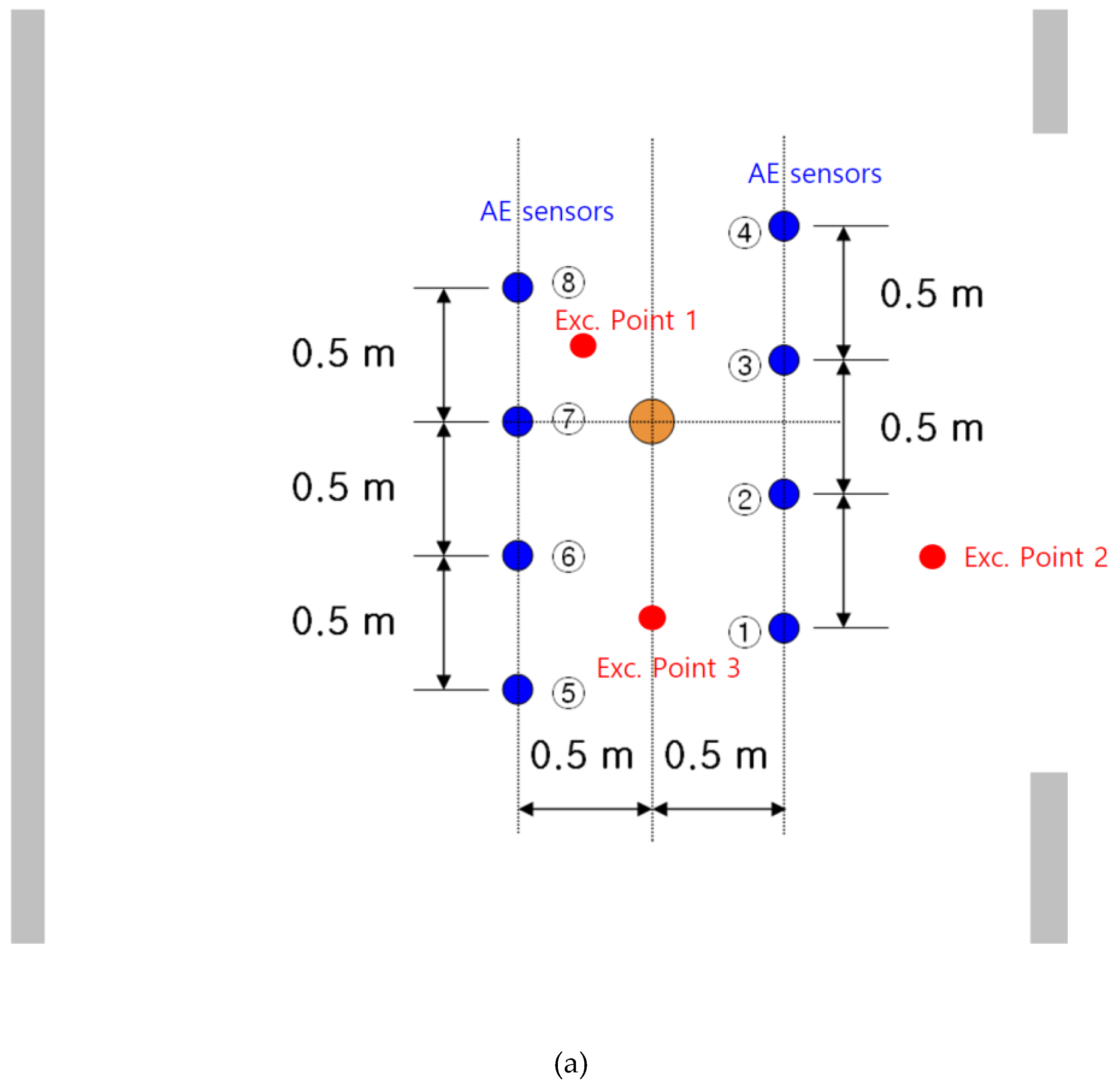
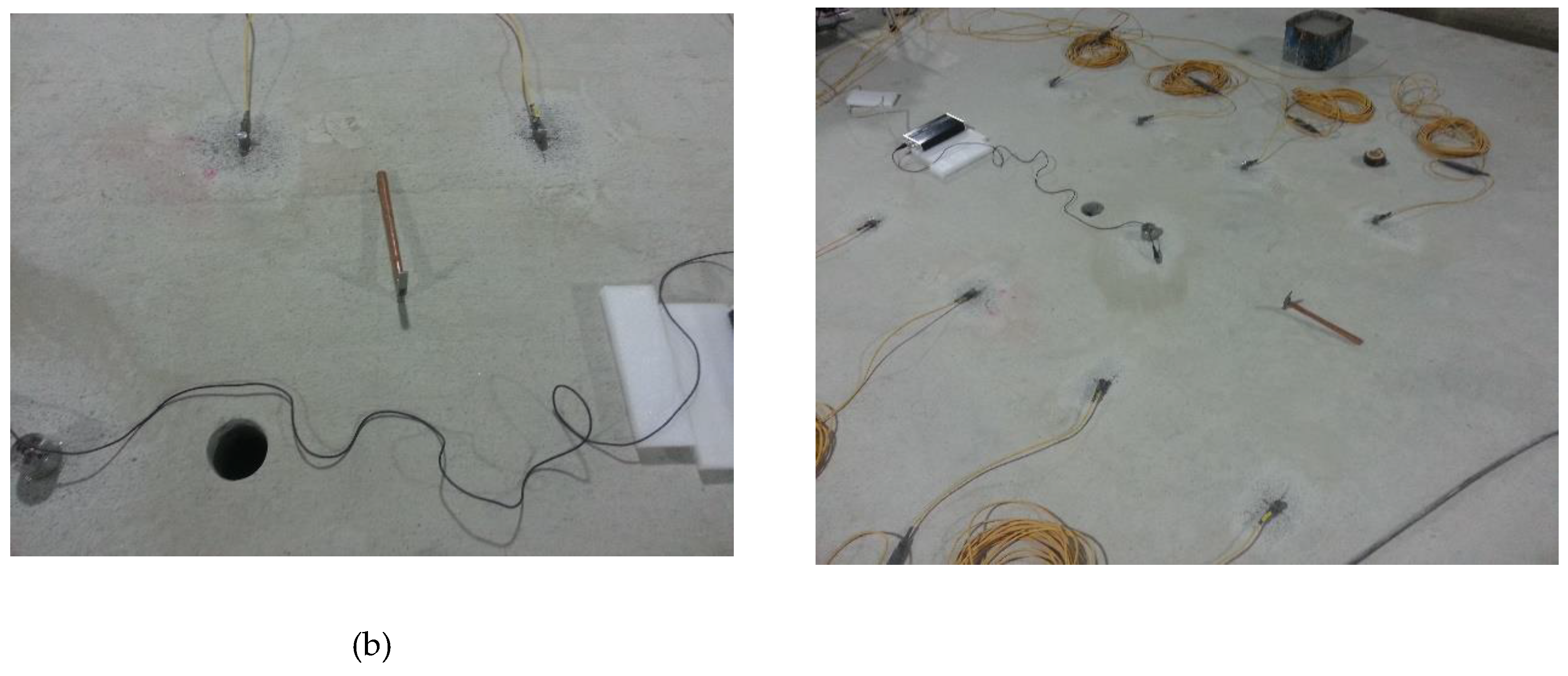
Figure 24.
(a) Signal results from each sensor, and (b) calculation of moving window when Exc. Point1 was excited with an impact hammer.
Figure 24.
(a) Signal results from each sensor, and (b) calculation of moving window when Exc. Point1 was excited with an impact hammer.
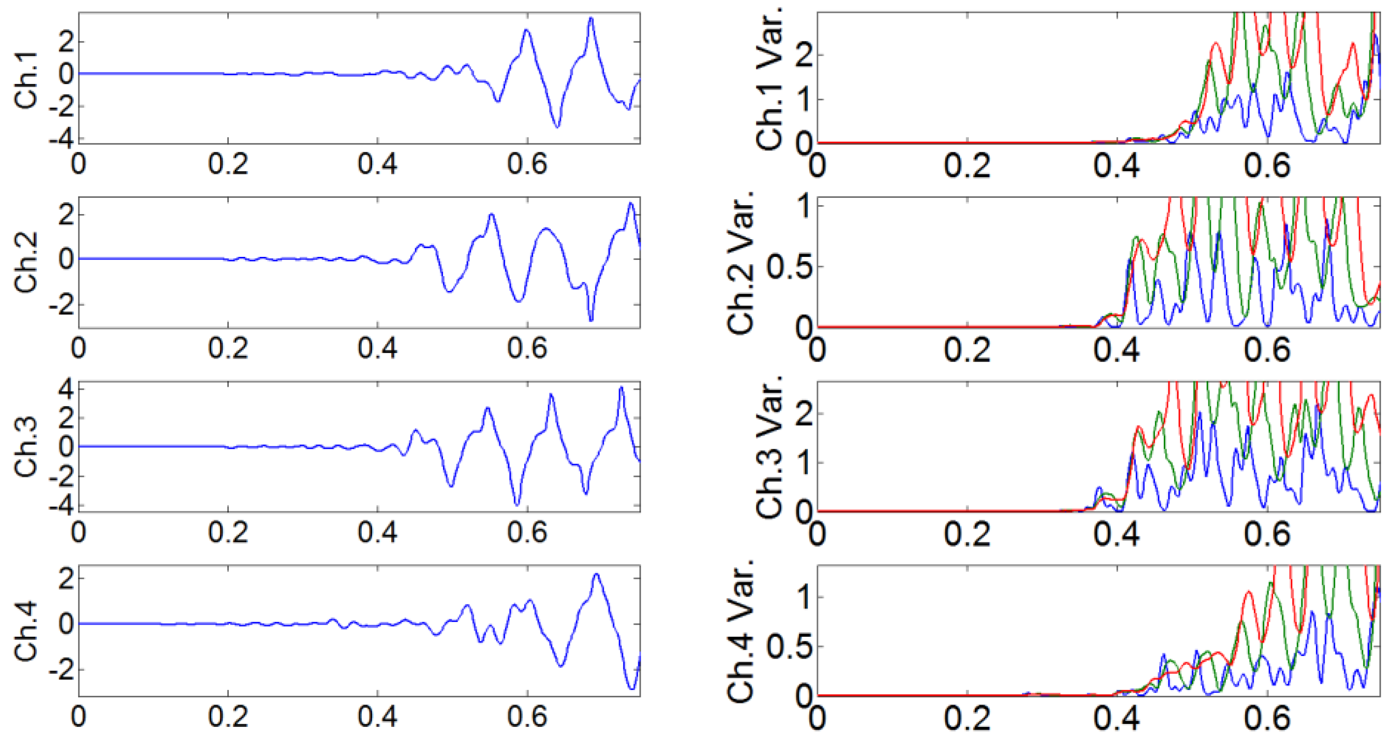
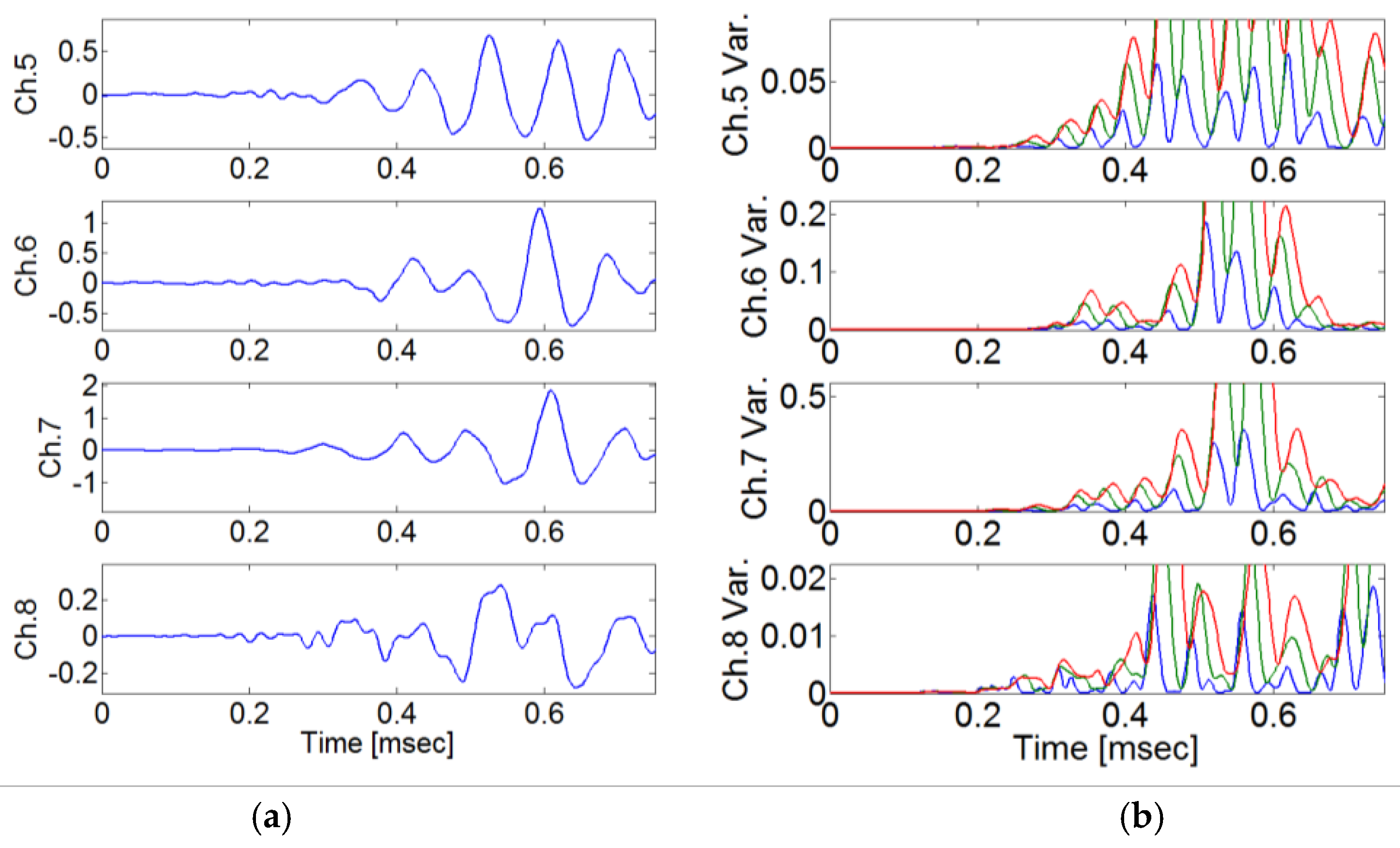
Figure 25.
Estimated impact location result. Exc. Point 1 location is (x,y)=(-0.25m,0.25m). Estimated location is (x,y)=(-0.267m,0.248m). The blue dots represent sensor locations, and the red dot represents the assumed source location.
Figure 25.
Estimated impact location result. Exc. Point 1 location is (x,y)=(-0.25m,0.25m). Estimated location is (x,y)=(-0.267m,0.248m). The blue dots represent sensor locations, and the red dot represents the assumed source location.
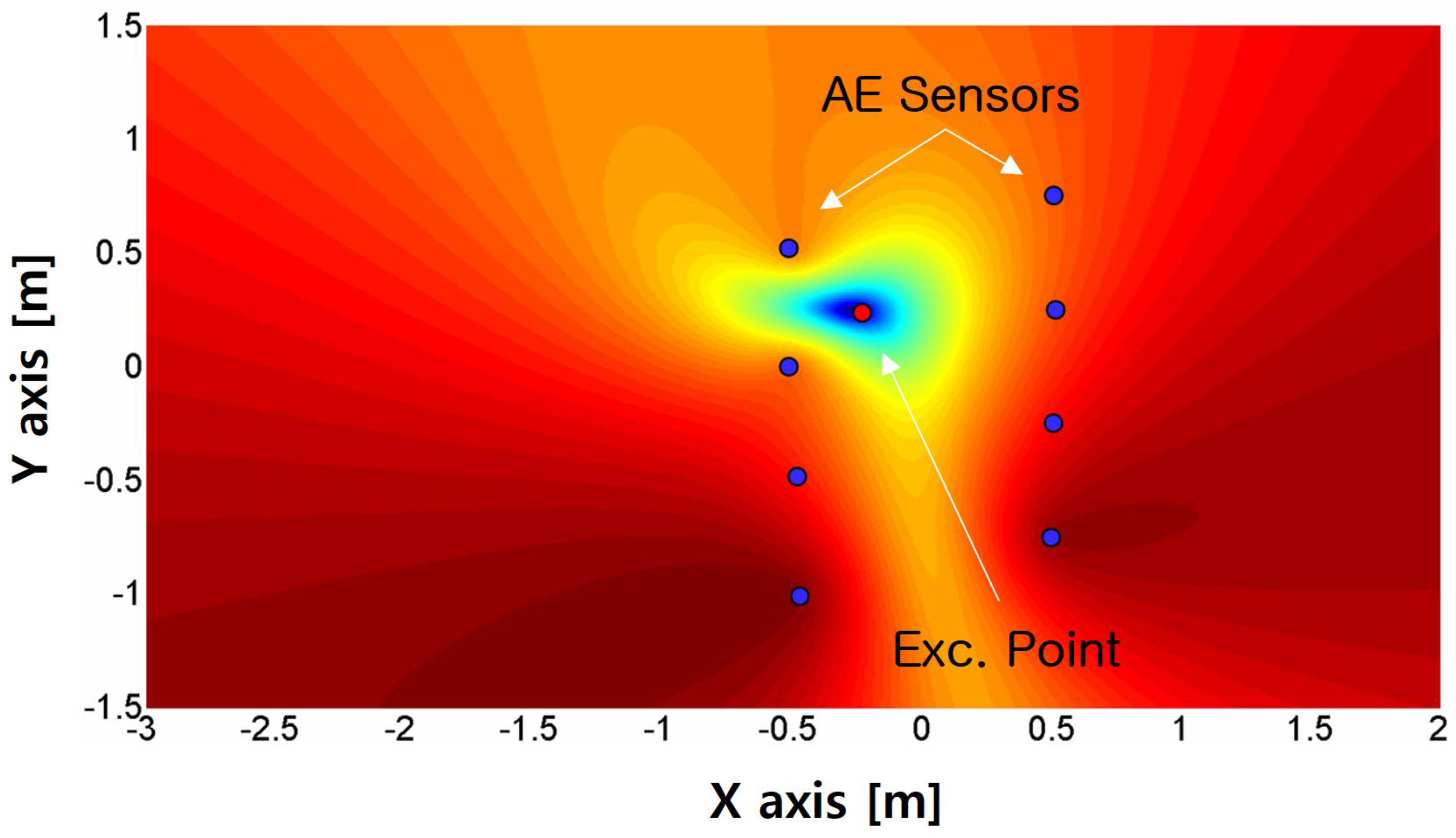
Figure 26.
Estimated impact location result. The Exc. Point 2 location is (x,y)=(1m,-0.5m). Estimated location (x,y)=(0.91m, 0.497m). The blue dots represent sensor locations, and the red dot represents the assumed source location.
Figure 26.
Estimated impact location result. The Exc. Point 2 location is (x,y)=(1m,-0.5m). Estimated location (x,y)=(0.91m, 0.497m). The blue dots represent sensor locations, and the red dot represents the assumed source location.
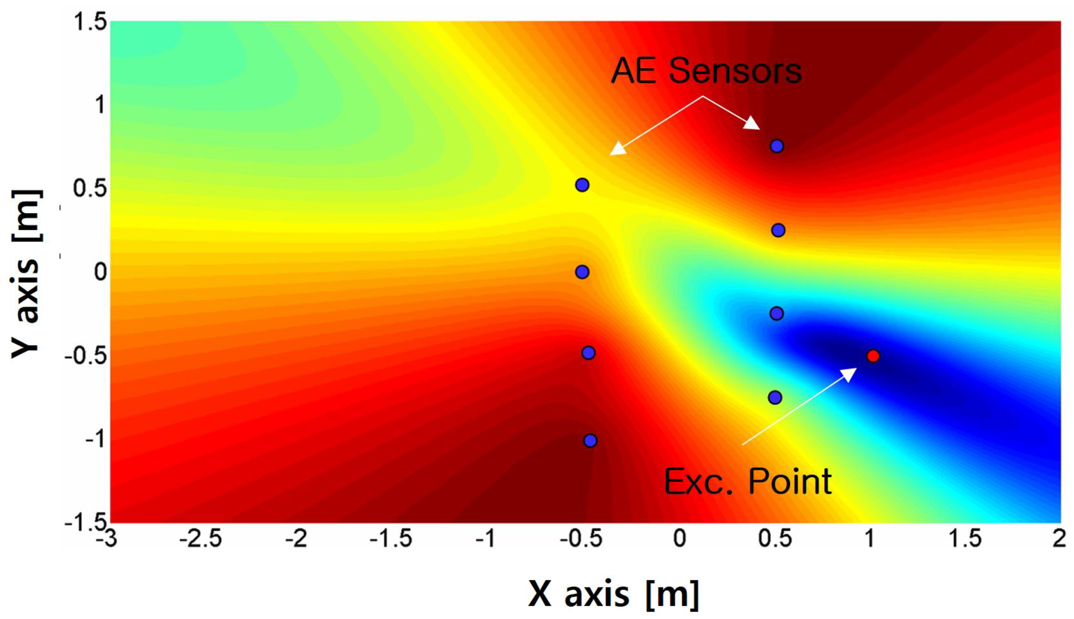
Figure 27.
Estimated impact location result. The Exc. Point 3 location is (x,y)=(0m,-0.75m). Estimated location (x,y)=(-0.032m,-0.704m). The blue dots represent sensor locations, and the red dot represents the assumed source location.
Figure 27.
Estimated impact location result. The Exc. Point 3 location is (x,y)=(0m,-0.75m). Estimated location (x,y)=(-0.032m,-0.704m). The blue dots represent sensor locations, and the red dot represents the assumed source location.
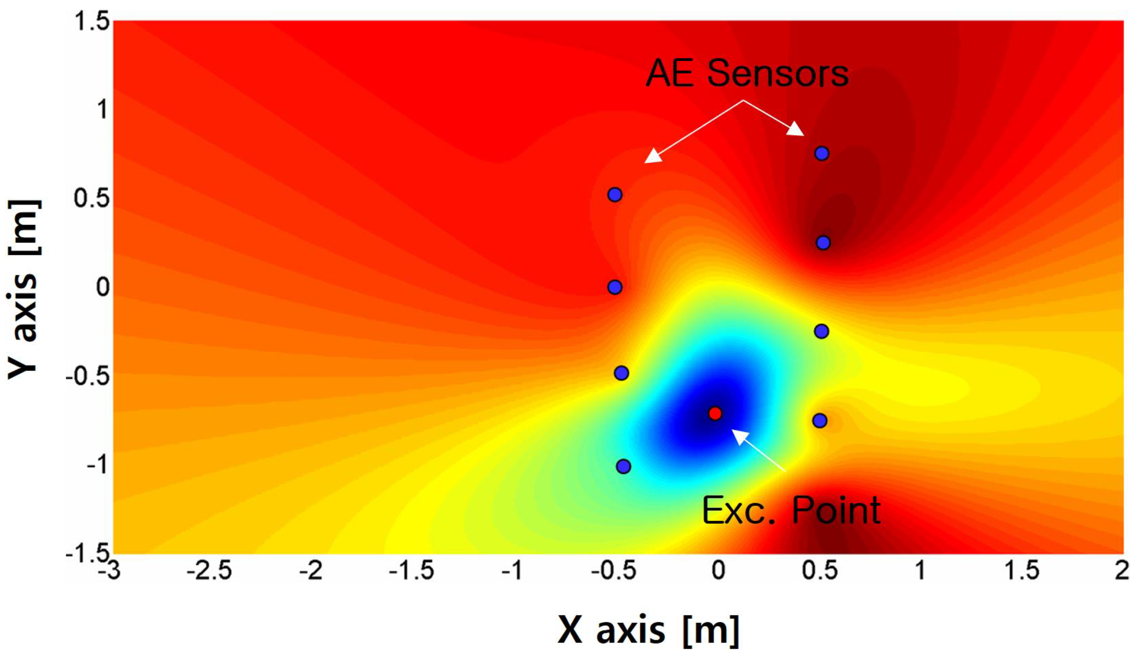

Table 3.
Measured arrival time; arrival delay time of each sensor channel depending on the source location.
Table 3.
Measured arrival time; arrival delay time of each sensor channel depending on the source location.
| True source locations (x,y,z) Unit : mm | |||
|---|---|---|---|
| (-125, 0, 50) | (0, 0, 50) | (125, 0, 50) | |
| Arrival time (msec) | Arrival time (msec) | Arrival time (msec) | |
| Ch.1 | 1.302 | 1.232 | 1.174 |
| Ch.2 | 1.304 | 1.236 | 1.175 |
| Ch.3 | 1.189 | 1.170 | 1.174 |
| Ch.4 | 1.190 | 1.170 | 1.176 |
| Ch.5 | 1.188 | 1.234 | 1.252 |
| Ch.6 | 1.191 | 1.235 | 1.254 |
Table 4.
Source localization results.
| Source locations (x,y,z) unit: mm | |||
|---|---|---|---|
| True source locations | (-125, 0, 50) | (0, 0, 50) | (125, 0, 50) |
| Estimated source locations | (125.8, 2.7, 50) | (-0.5, 0.5, 50) | (-124.7, 1.5, 50) |
Table 1.
Signal characteristics of crack waves and noise.
| Crack wave | Noise | |
|---|---|---|
| Time domain | Higher magnitude. | Lower magnitude |
| Frequency domain | Distribution with a narrow band | Distribution with a wide band |
Table 2.
Locations of the AE sensors used for source localization.
| Sensor | X(mm) | Y(mm) | Z(mm) |
|---|---|---|---|
| No. 1 | -250 | 100 | 50 |
| No. 2 | -250 | -100 | 50 |
| No. 3 | 0 | 100 | 50 |
| No. 4 | 0 | -100 | 50 |
| No. 5 | 250 | 100 | 50 |
| No. 6 | 250 | -100 | 50 |
Table 5.
True excited location and location estimated from impact signal.
| True Location (x,y) | Estimated Location (x,y) | |
|---|---|---|
| 1 | (-0.25 m, 0.25 m) | (-0.267 m, 0.248 m) |
| 2 | (1.50 m, 0.0 m) | (1.69 m, 0.003 m) |
| 3 | (0 m, -0.75 m) | (-0.032 m, -0.704 m) |
Disclaimer/Publisher’s Note: The statements, opinions and data contained in all publications are solely those of the individual author(s) and contributor(s) and not of MDPI and/or the editor(s). MDPI and/or the editor(s) disclaim responsibility for any injury to people or property resulting from any ideas, methods, instructions or products referred to in the content. |
© 2024 by the authors. Licensee MDPI, Basel, Switzerland. This article is an open access article distributed under the terms and conditions of the Creative Commons Attribution (CC BY) license (http://creativecommons.org/licenses/by/4.0/).
Copyright: This open access article is published under a Creative Commons CC BY 4.0 license, which permit the free download, distribution, and reuse, provided that the author and preprint are cited in any reuse.


