Submitted:
03 September 2024
Posted:
04 September 2024
You are already at the latest version
Abstract
Monitoring seaweed growth rates and biomass is crucial for optimizing harvest strategies in aquaculture systems. While such a task can be performed manually on a small farm, such as the Integrated Multi-Trophic Aquaculture (IMTA) system at Harbor Branch Oceanographic Institute at Florida Atlantic University (HBOI), a commercial farm will have to rely on the automated sensor to perform such a task. This study introduces an advanced LSTM-based approach for forecasting seaweed growth and biomass. Utilizing a combination of real and synthetic data, LSTM models are trained and evaluated for their predictive performance. Synthetic sensor data was generated using mathematical equations that simulate realistic aquaculture conditions, with added noise to reflect sensor variability. Building on the foundation of the Pseudorandom Encoded Light for Evaluating Biomass (PEEB) sensor deployed at the seaweed tank in the HBOI IMTA system, we refine the process of biomass estimation by introducing non-linear regression models for predicting seaweed growth and biomass. The results showed that the LSTM model trained with a loss function under physics constraint, combining MSE and physical laws, outperformed models trained with MSE alone, achieving a significantly lower error in predicting seaweed growth. The variation trend of the predicted biomass from the network matched well with the sensor measurement after moving average preprocessing, demonstrating the robustness of the proposed technique in handling noisy sensor data. This study highlights the potential of integrating machine learning with physical models to optimize seaweed cultivation and support sustainable aquaculture practices.
Keywords:
Integrated Multi-Trophic Aquaculture (IMTA)
; seaweed growth prediction
; Long Short-Term Memory (LSTM)
; loss function under physics constraint
; deep learning
; synthetic data generation
; sensor data augmentation
; aquaculture optimization
; biomass estimation
; environmental monitoring
; Robotic System
1. Introduction
Aquaculture, the farming of aquatic organisms, exhibits significant diversity in methods, species, and systems, ranging from traditional ponds to sophisticated Recirculating Aquaculture Systems (RAS) and open-water cultures. In particular, RAS employs a controlled environment where water is recycled and reused after mechanical and biological filtration and removal of suspended matter and other wastes. One attractive feature of RAS is that the farm is insulated from external environmental and climatic influence, therefore it can operate with fewer geographical constraints than pond or offshore farms. However, RAS typically consumes more energy and has less efficient nutrient utilization compared to Integrated Multi-Trophic Aquaculture (IMTA). Since 2012, Harbor Branch Oceanographic Institute at Florida Atlantic University (HBOI) has been at the forefront of developing land-based marine Integrated Multi-Trophic Aquaculture (IMTA) systems [1]. IMTA facilitates a symbiotic co-culture of various species, where the waste products of one serve as resources for another, enhancing system efficiency and sustainability. Compared with traditional RAS solutions, IMTA provides superior energy efficiency and water utilization, as it leverages the natural biological interactions among species to recycle nutrients and reduce waste. The innovative IMTA system at HBOI includes species such as fish, shrimp, urchins, oysters, and macroalgae, also known as seaweed.
Seaweed is a critical component in the IMTA system at HBOI. Seaweed such as sea lettuce (Ulva lactuca) grows fast and can be harvested within several days. The seaweed growth has to be monitored regularly to ensure proper nutrient levels in the tank are maintained. Seaweed is particularly well-suited for monitoring because of its short growth cycle and relatively simple requirements for basic monitoring, making it an ideal starting point for testing the IMTA system. Currently, technicians need to physically examine the seaweed, which is labor-intensive and time-consuming. While this may be only a nuisance for a small research IMTA system at HBOI, which operates eight seaweed cultivation tanks, the labor cost to manually inspect seaweed biomass will be prohibitively high on a commercial-scale farm. Such farms may operate hundreds or thousands of such tanks. In this regard, an Internet of Things (IoT) framework is being developed in the HBOI IMTA system, leveraging the success of the Hybrid Aerial Underwater Robotic System (HAUCS) project, which aims to develop an IoT solution for pond aquaculture farms [4]. In particular, a cloud-based decision support system that integrates data from the in-situ sensors and weather station. The collected data is stored in a central database (Firebase), where it is analyzed to predict and address potential issues before they affect water quality in the farm.
Previous research introduced the Pseudorandom Encoded Light for Evaluating Biomass (PEEB) sensor, designed to measure seaweed biomass automatically within the HBOI IMTA system [2]. This sensor, utilizing commercially off-the-shelf (COTS) components, demonstrated a cost-effective and reliable method for biomass measurement.
However, the current practice still faces challenges, including limited sensor calibration, short deployment duration, and the labor-intensive process of physically examining seaweed [2]. Figure 1 provides an overview of the IMTA system, illustrating its framework and layout.
To improve biomass estimation, previous efforts applied non-linear regression models to predict seaweed biomass and optimize harvest timing. Although this approach demonstrated the potential for estimating seaweed biomass, the limited amount of data available for regression analysis resulted in high error margins [3]. The scarcity of comprehensive data highlighted the need for more advanced data modeling techniques.
To address the ongoing challenges of data scarcity and enhance predictive capabilities, this study focuses on advancing the methodology for seaweed growth prediction by integrating sensor data with advanced machine learning models. One of the key challenges in this application is the limited availability of training data, which is a common issue not only in aquaculture but also in many other adjacent fields, such as agriculture. In our case, the ground truth for seaweed biomass is only available at discrete intervals: the initial weight at the start of cultivation, the final harvest weight, and partial weekly harvest weights. No direct measurements of biomass are available between these points, making it difficult for the model to learn from continuous ground truth data. This lack of real-time ground truth information poses a significant challenge, as the model must rely heavily on indirect environmental factors and sparse sensor readings to predict the seaweed growth trajectory over time. Specifically, we aim to develop and evaluate a novel LSTM-based approach that can effectively leverage both real and synthetic data to achieve high accuracy and reliability in predicting seaweed growth rates and biomass under such constraints.
The two main contributions of this paper are:
- Synthetic Data Generation: Due to the scarcity of real-world data, we generate synthetic sensor data based on real weather conditions and water quality measurements. This synthetic data is created using mathematical equations that simulate realistic aquaculture conditions, with added noise to reflect sensor variability. This approach ensures a robust training dataset for the predictive model.
- Sequential Model Prediction with LSTM with Physics Constraint Loss Function: The LSTM model is developed to predict seaweed growth rates and biomass. The model is trained using the augmented dataset, combining real and synthetic data, and evaluated for its predictive performance. Additionally, the study explores the use of Physics Constraint Loss Functions, which integrate traditional MSE loss with physical laws, to enhance prediction accuracy and model robustness.
By building upon existing methods and introducing synthetic data generation alongside advanced sequential modeling, this research aims to significantly improve the accuracy and reliability of seaweed biomass predictions, contributing to more sustainable aquaculture practices.
2. Background and Related Works
In the advancement of seaweed biomass prediction, understanding the role of sensor technology and appropriate modeling techniques is crucial. This section reviews related work on integrating sensors for environmental monitoring in aquaculture, as well as the application of machine learning and hybrid models to improve prediction accuracy. These foundational approaches inform the development of more robust predictive systems for optimizing seaweed growth in IMTA systems.
2.1. Advanced Sensor Technology in Aquaculture
The integration of advanced technologies for biomass estimation and system optimization is crucial in modern aquaculture. The development of IMTA systems has marked a significant shift towards sustainability and efficiency by leveraging symbiotic relationships among species. At the HBOI, the PEEB sensor has been developed to automate and refine biomass monitoring processes, showcasing the potential of cost-efficient, compact, and energy-efficient sensors for commercial-scale IMTA farms [1,2,3].
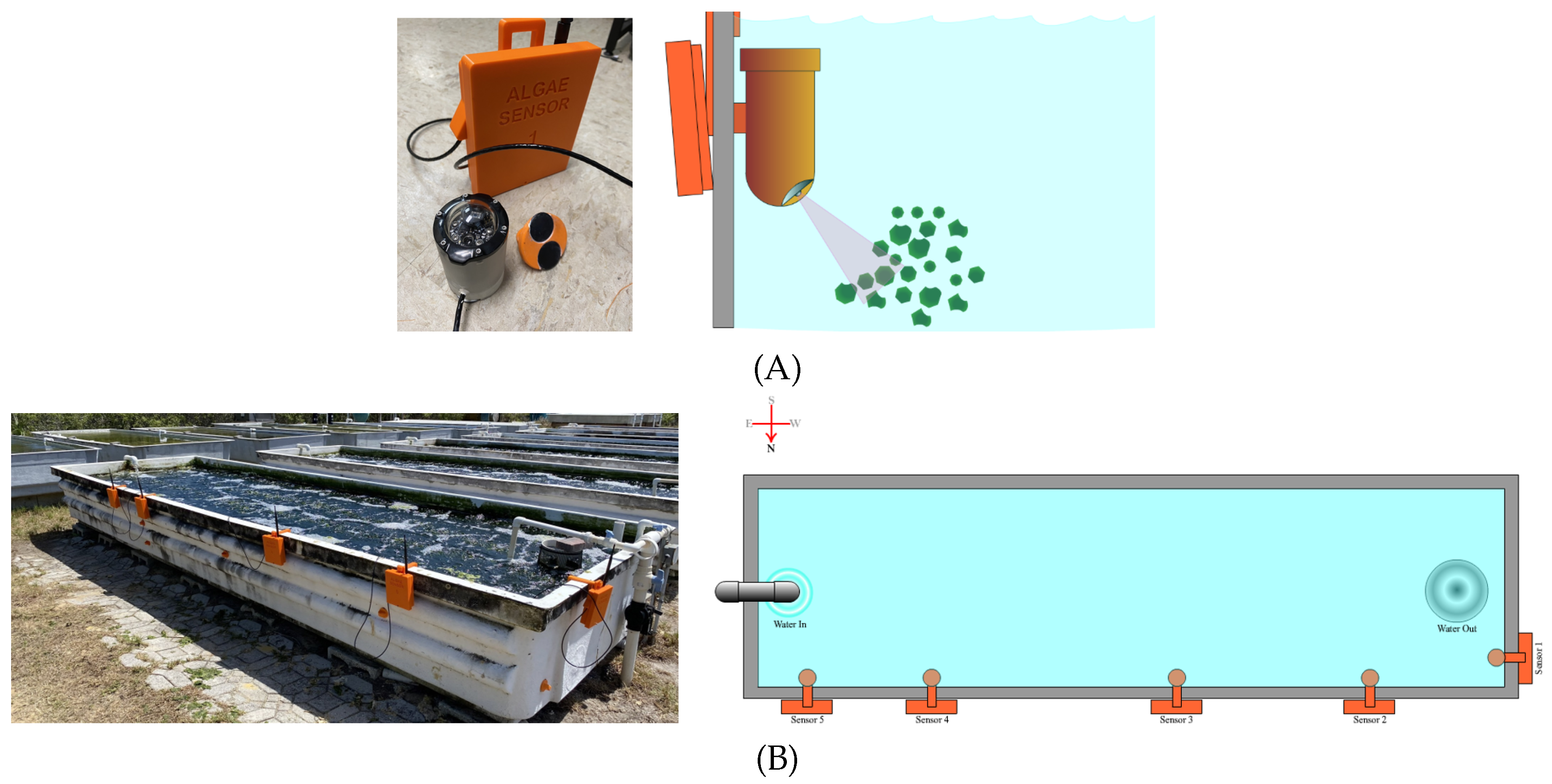
To optimize data collection, IR sensors were installed underwater at a forty-five-degree angle towards the tank’s bottom, minimizing inteference from external light sources. The tanks, measuring 5.5 meters in length, 1.5 meters in width, and 1.0 meter in height, provided a total volume of 8.25 cubic meters. The initial biomass for each cycle was set at 22.11 kg. Data was collected every 11 minutes and uploaded to a Firebase database via LoRA wireless link [5], ensuring comprehensive and reliable datasets for analysis. Figure 2 shows the structure of the sensor and its installation in the water tank.
Restocking events were systematically documented to ensure consistent baseline data for each growth cycle, while weekly harvest weights, measured every Thursday, provided periodic insights into the growth progression. A comprehensive harvest every three months allowed for an extensive evaluation of the seaweed biomass. The data collection process, enhanced by a Golay pulse compression technique to improve the signal-to-noise ratio and reduce the interference from ambient light [6]. The sensor readings were calculated using the formula:
2.2. Modeling Seaweed Growth
Modeling seaweed growth is critical to optimizing biomass prediction in IMTA systems. This study utilizes a comprehensive approach integrating environmental and biological factors to accurately simulate seaweed biomass growth. The methodology follows the principles outlined by Jayaraman and Rhinehart (2015) for algae growth modeling [7]
2.2.1. Incident Light and Photosynthesis
To simulate seaweed biomass growth accurately, the incident light intensity, specifically photosynthetically active radiation (PAR) light, is crucial for photosynthesis. Its attenuation in water is modeled by the Beer-Lambert law:
where represents the maximum incident light intensity (W/m2), and is the extinction coefficient. Photosynthetic rate.
The photosynthetic rate P is further described by:
where is the maximum photosynthetic rate, and k is a fitting parameter.
2.2.2. Temperature Effect
Temperature affects growth, modeled by a Gaussian function centered around the optimal temperature :
where T is the water temperature (K) and is the standard deviation.
2.2.3. Nutrient Concentration
The Monod equation models nutrient-dependent growth, particularly nitrogen availability:
where C is the nutrient concentration, and is the half-saturation constant.
2.2.4. von Bertalanffy Growth Function
The von Bertalanffy growth function (VBGF) [8]. is applied to model the growth rate of seaweed biomass:
where L is the current biomass concentration (g/L), is the asymptotic biomass concentration, and k is the growth rate constant. This function accounts for decelerating growth as biomass approaches saturation.
These models combine to provide a comprehensive framework for simulating seaweed growth under varying environmental conditions.
2.3. Sequential Model Networks Overview
Sequential model Networks have been pivotal in handling data where the order of inputs needs to be preserved, such as in time series forecasting and natural language processing (NLP). These networks excel in predicting sequences where the input is not fixed but varies in length and content.
Early work on sequential model Networks began with Recurrent Neural Networks (RNNs), which are capable of learning temporal dependencies in data. However, RNNs face limitations in handling long sequences due to the vanishing gradient problem, making it difficult for them to learn long-term dependencies [9]. To address these limitations, Long Short-Term Memory (LSTM) networks were developed, introducing forget gates that allow the network to decide what information to retain or discard [10].
LSTM networks have been further enhanced and adapted into various architectures for specific tasks, showing remarkable success in sequential data prediction [11]. Despite these advancements, LSTM networks can still be computationally intensive and challenging to train over very long sequences [24,25,26,27,28].
2.4. Sequential Model Networks for Forecasting and Prediction
Sequential model networks have proven indispensable in time series forecasting because of their ability to learn from the temporal structure and dependencies within data. These networks excel at identifying patterns across time, which is essential when predicting future values based on historical data. Their strength lies in the fact that they can capture both short-term fluctuations and long-term trends, making them well-suited for handling time series data in a wide range of applications.
Over the years, various sequential model networks have been explored. Traditional statistical methods, such as Autoregressive Integrated Moving Average (ARIMA) and Exponential Smoothing, have long been the standard for time series forecasting. However, while these methods are useful for linear patterns and smaller datasets, they struggle with the complexity of large, non-linear, and highly variable datasets often found in modern applications like aquaculture monitoring.
In response to these challenges, advanced deep-learning methods have emerged. One such networks is DeepAR [13], a probabilistic forecasting method that employs autoregressive recurrent neural networks to generate probabilistic predictions. DeepAR has the advantage of learning from multiple time series at once, providing a distribution over possible future outcomes instead of single-point estimates, which is particularly useful for applications with inherent uncertainty, like environmental modeling.
Another notable advancement is Temporal Convolutional Networks (TCNs) [14]. Unlike traditional RNNs, which rely on sequential processing, TCNs use dilated causal convolutions, allowing them to capture long-range dependencies in time series data more efficiently. This makes them not only faster to train but also more accurate in scenarios where long-term context is important for making predictions, such as predicting seaweed growth rates over extended periods.
More recently, the introduction of attention mechanisms in model networks like Temporal Fusion Transformers (TFTs) [15] has brought significant improvements to the field of time series forecasting. Attention mechanisms allow the network to selectively focus on the most relevant parts of the input sequence, dynamically weighting these inputs based on their importance to the forecast. This improves both interpretability and accuracy, as the network can highlight which variables or time steps contribute most to the prediction. This is particularly beneficial in cases where the data contains multiple input variables (e.g., environmental factors like solar radiation, air temperature, and humidity), and not all inputs are equally relevant at all times.
Other research [29,30,31,32,33,34] has further demonstrated that combining sequential model networks with attention mechanisms can yield state-of-the-art results in time series forecasting. These models are designed to be robust even when data is noisy, incomplete, or exhibits complex dependencies, which are common challenges in real-world aquaculture data. By integrating such approaches, forecasting accuracy can be significantly improved, providing more reliable predictions for tasks such as seaweed growth in IMTA systems.
2.5. Sequential Model Networks for Aquaculture
In aquaculture, accurately predicting environmental conditions and biological processes is essential for improving operational efficiency and sustainability. Sequential model networks, especially those designed for time series forecasting, have become increasingly valuable in this domain due to their ability to learn from temporal dependencies in data.
Traditionally, networks such as Autoregressive Integrated Moving Average (ARIMA) have been used in aquaculture for forecasting environmental parameters like water temperature, dissolved oxygen, and nutrient levels. These networks are effective for linear relationships and small datasets but tend to struggle with non-linear, highly variable data, which are common in aquaculture settings. For example, ARIMA has been applied to predict water quality parameters like temperature and dissolved oxygen in both freshwater and seawater systems but exhibited limitations when dealing with more complex environmental conditions [18,35].
Recent advances in deep learning, particularly Recurrent Neural Networks (RNNs) and Long Short-Term Memory (LSTM) networks, have introduced a new level of accuracy and flexibility for aquaculture applications. LSTM networks are particularly suited for aquaculture because they can capture both short-term fluctuations and long-term trends in environmental variables, such as water quality and temperature, directly affecting fish growth and health. These networks have been used to predict complex biological outcomes, such as fish biomass and feed consumption, by learning from sequential environmental data and adapting to the high variability often observed in aquaculture environments [36].
Moreover, some studies have employed hybrid approaches, combining sequential model networks with physical laws or empirical models to enhance prediction accuracy. For instance, hybrid models incorporating LSTM with physical laws governing water flow and nutrient absorption have outperformed traditional methods when predicting the growth of aquatic species [37]. Including domain-specific knowledge helps compensate for the sparse and irregular training data commonly encountered in aquaculture, where ground truth is only available at discrete time intervals, such as before and after harvest.
Despite these advancements, sequential model networks in aquaculture still need to improve, particularly with training data scarcity. Unlike continuous real-time monitoring, ground truth data (such as seaweed biomass or fish weight) is often available only at key intervals, such as the start of the cultivation cycle and at harvest. This makes it difficult for the networks to accurately capture the in-between growth dynamics. Techniques such as data augmentation and synthetic data generation have been explored to address this gap, with some success [38]. However, the reliance on synthetic data introduces uncertainty, especially when environmental conditions change unpredictably or when the biological species being cultivated have variable responses to these conditions.
Therefore, it is crucial to develop more sophisticated networks that can better handle the sparse nature of real-world data. Techniques like Temporal Convolutional Networks (TCNs) and Temporal Fusion Transformers (TFTs) have the potential to further improve predictive accuracy by selectively weighting relevant inputs and learning from multiple time series simultaneously. These methods offer robust solutions for handling incomplete, noisy, and high-dimensional datasets, making them well-suited for aquaculture [13,14,15].
2.6. Physics Constraint in Neural Network
Hybrid loss functions, which combine multiple objectives, are increasingly recognized as powerful tools in neural networks, particularly in scenarios where both empirical data and theoretical constraints play a crucial role. These functions allow networks to balance learning from real-world data while respecting underlying physical or domain-specific laws, ensuring that predictions adhere to known behaviors even when data is noisy, sparse, or incomplete. In environmental monitoring and agriculture fields, hybrid loss functions have been applied effectively, enhancing networks robustness and generalization across different datasets.
One significant advantage of hybrid loss functions is their ability to mitigate the overfitting often occurring when networks are trained solely on noisy or limited datasets. By introducing a secondary loss component based on physical laws, the networks is guided to respect known behaviors, even when the data itself may be incomplete or inconsistent. This results in networks that generalize better across different datasets and perform more reliably under various conditions [16,17].
Lutter et al. [17] applied a hybrid loss in control theory, integrating physics constraints into reinforcement learning models. By doing so, the networks maintained system stability while optimizing performance. This demonstrates the broader applicability of physics-constrained neural networks in domains that require adherence to physical laws. Moreover, this approach enabled the network to deal with cases where data might be sparse or incomplete.
This study applies a hybrid loss function to ensure the LSTM model captures both real sensor measurements and ideal seaweed growth patterns governed by physical laws. The hybrid loss function used is:
where is the weighting factor that balances the contribution of sensor data and physical growth laws. represents the actual biomass measurements, denotes the theoretical biomass values calculated from growth models, and is the predicted biomass.
If is set too high, the network relies too heavily on real-world data, resulting in predictions that do not align with theoretical laws, particularly in noisy or sparse data. Conversely, if is set too low, the network overemphasizes theoretical principles, potentially ignoring external factors that could influence the outcome. The optimal value of strikes a balance, allowing the network to account for both empirical measurements and underlying growth dynamics. This balance helps the network "fill in the gaps" when sensor data is unavailable by leaning on theoretical networks to maintain prediction accuracy.
Hybrid loss functions have been widely explored in agriculture and environmental monitoring, where sensor data is often subject to noise and interruptions. The hybrid loss function not only ensures that the network learns from available real-world data but also allows it to "fill in the gaps" during periods where real data is missing or sparse. For instance, Omer et al. [18] demonstrated the effectiveness of hybrid models combining neural networks with autoregressive techniques for water quality prediction. Similarly, Bai et al. [19] employed a hybrid deep learning model in smart agriculture to improve the accuracy of climate data prediction. Furthermore, Ojo et al. [20] explored the use of deep learning networks for predicting crop growth in controlled environments, showcasing the potential of combining physical laws with neural networks. Additionally, Nordin et al. [21] reviewed the use of wireless sensor networks and hybrid models in precision agriculture, highlighting the importance of integrating theoretical knowledge to improve the reliability of environmental data-driven models.
By incorporating physical constraints and real-world data, hybrid loss functions offer a powerful approach to improving network accuracy and robustness, making them particularly valuable in domains where direct measurement (i.e. training data) is challenging, but theoretical models can provide essential guidance.
3. Materials and Methods
This section describes the data collection, network architecture, and training methods used in this study. A combination of real and synthetic data was employed to simulate environmental conditions for seaweed growth. The LSTM model was chosen after evaluating several different techniques, as it proved to be the most effective in handling this process. Critically, hybrid loss functions were employed to integrate empirical measurements with physical growth models. Preprocessing and evaluation techniques were also applied to ensure accurate predictions. The following subsections detail each component.
3.1. Data Collection
The data collection process in this research is divided into two main cases: collecting sensor data from operational seaweed tanks for testing purposes and collecting data to generate synthetic data for training. The details of the data collection process are as follows:
3.1.1. Weather Data Collection
We collected weather condition data from the SenseStream website by selecting the HBOI AQUA 1 sensor [39]. The weather data collected includes date and time, air temperature, photosynthetically active radiation (PAR) data, humidity, precipitation intensity (mm/h), and total precipitation (millimeters). This data was collected at 5-minute intervals to support the prediction and to generate synthetic data for training purposes.
3.1.2. Collecting Real Data for Testing
The collection of real data for testing is based on the data collection methods described in previous research [3], with the following details:
- Data Collected from Sensors: Real data was systematically collected from May 2023 to January 2024, covering three complete cultivation cycles. Infrared (IR) sensors captured readings every 11 minutes, providing a comprehensive dataset essential for precise predictive modeling of seaweed growth. The data collection process included detailed documentation of restocking and harvesting, with initial seaweed weights serving as benchmarks and weekly harvest weights offering insights into growth progression. A Golay smoothing technique was applied to the sensor data to minimize noise and correct potential errors, enhancing the accuracy of the collected data.
- Restocking and Harvesting Schedules: Restocking events were documented to ensure baseline data reliability, while weekly and quarterly harvests provided consistent insights into seaweed growth and overall productivity. This structured data acquisition was crucial for evaluating cultivation methods and biomass viability.
From the data collected, we obtained time-stamped sensor data calculated as well as restocking and harvesting information measured in kilograms. The sensor data and harvesting weights were combined with weather data. However, since the timestamps of the weather and sensor data do not align, the sensor timestamps were used as the primary reference, with the closest weather data timestamps being matched accordingly.
Of the eleven collected datasets, five were incomplete due to missing early-stage data, leaving six usable datasets. Since this is insufficient for training deep learning models, synthetic data was generated to supplement the real data.
3.1.3. Nutrient and Water Temperature Data Collection for Data Generation
The prediction of seaweed growth can be significantly influenced by water quality and nutrient data. However, in practice, daily measurements of water quality are often not feasible, limiting their direct use in training models. Nevertheless, this data is valuable for generating synthetic data for training purposes.
Nutrient and water temperature data were recorded daily, including total ammonia nitrogen (TAN), nitrite, nitrate, pH, and water temperature. Missing data due to manual measurements was processed using the Kalman filter [22], a recursive algorithm that estimates system states from noisy and incomplete measurements.
The Kalman filter operates in two steps: prediction and update. The prediction step estimates the current state of the system based on previous data, while the update step refines the estimate using new observations. This allowed for accurate interpolation of missing nutrient and temperature data, which was then combined with weather data to generate synthetic datasets for training. 1
3.2. Seaweed Growth Synthetic Dataset
The synthetic data generated for seaweed growth is based on the measurements of nutrients, solar irradiance, and water temperature—factors directly influencing the biological processes of seaweed growth. We also incorporated environmental factors such as solar radiation, rainfall, and air temperature to train the predictive network, alongside sensor values. While these environmental variables do not directly measure seaweed growth, they are more suitable for real-time prediction due to their continuous availability through the weather station.
The process of data generation for seaweed growth simulation follows the modeling techniques described in Section 2.2, with adjustments made to align with the available data.
To generate realistic seaweed growth rates, the following model parameters were controlled:
- Tank Dimensions: The seaweed is cultivated in tanks measuring 1.5 meters in width, 5.5 meters in length, and 1 meter in depth, providing a total volume of 8.25 m3.
- Initial Biomass: The initial seaweed biomass at the start of cultivation is 22.11 kg, corresponding to a concentration of 2.68 g/L.
- Cultivation Period: Seaweed is cultivated for 8 weeks, with weekly harvests except in the final week. Harvest weights follow a normal distribution with a mean of 18.5 kg, constrained between 12 kg and 25 kg. In approximately 5% of cases, no harvesting occurs.
- Optimal Environmental Conditions: The optimal growth temperature is 24.86°C, with an ideal pH of 8.1. Maximum solar radiation, recorded by sensors, is 1430 W/m2.
- Asymptotic Biomass Concentration: The saturation biomass concentration in the tank is 90 kg, resulting in an asymptotic biomass concentration of 10.91 g/L.
These parameters were used to compute the seaweed growth rate, incorporating real-time solar irradiance data from the weather station. Figure 3 illustrates the simulated seaweed growth rate over an eight-week period.
Once the growth rate data was generated, it was converted into sensor readings. The IR sensors used to measure biomass are sensitive to seaweed density, where higher density results in higher sensor readings. Due to the inherent noise in IR sensors, normal noise was added to the simulated growth rate to mimic realistic sensor behavior. The growth rate was converted into sensor values using the equation:
where w is the average sensor calibration factor and b is the minimum sensor reading. Figure 4 shows the results after converting the seaweed growth rate into sensor data.
3.3. Network Architecture
The network employed in this study is based on the LSTM architecture. The LSTM network is particularly well-suited for sequential data and time series prediction due to its ability to capture long-term dependencies. The input to the network consists of eight features: timestamp, sensor, air temperature, solar radiation, humidity, precipitation intensity, total precipitation, and harvest weight. These features are derived from sensor measurements and environmental data, making them critical for predicting seaweed mass in the tank at any given time.
The LSTM network comprises five layers, each with a hidden size of 64. The network takes in the eight input features and processes them through the LSTM layers, ultimately producing a single output: the predicted seaweed mass in the tank at the current time step.
Figure 5 provides a schematic representation of the LSTM model architecture, showcasing the stacked layers and the internal flow of information within the network.
3.4. Injecting Physical Constraint in the Loss Function
We employed a hybrid loss function for the training process to enhance the network’s predictive accuracy. Initially, the model was trained using only the Mean Squared Error (MSE) loss function (), which is commonly used for regression tasks where the objective is to minimize the difference between the predicted and actual seaweed mass at the final time step. However, this approach yielded suboptimal results as it failed to capture the full relationship between seaweed mass, sensor data, and environmental variables across the entire cultivation period.
To address this limitation, we introduced a loss function with physical constraint (), which is based on ideal growth rates derived from the physical laws governing seaweed growth. This ideal growth rate was computed at each time step and combined with the MSE loss function to create the hybrid loss function. The hybrid loss helps the network better align with the biological dynamics of seaweed growth throughout the cultivation cycle.
Various values of were tested (0.5, 0.7, 0.8, 0.9, 0.95) to balance the MSE loss with the physical loss, where represents the weight of the MSE loss. This allowed us to experiment with different levels of influence between the actual sensor data and the physical growth model. The training aimed to optimize to achieve the best balance between these two components for accurate prediction of seaweed growth dynamics.
As a result, the network provides accurate predictions of final seaweed biomass and understands growth dynamics, allowing for proactive interventions, such as harvesting recommendations. This hybrid loss approach is particularly valuable for monitoring seaweed growth continuously over time, ensuring optimized aquaculture management.
Figure 6 shows the hybrid loss function used in the LSTM model, integrating both physical loss and Mean Squared Error (MSE) loss for optimal prediction accuracy in seaweed growth estimation. The physical loss is calculated as:
where represents the ideal weight of seaweed at each time step, calculated from the theoretical growth model, is the predicted weight of seaweed at each time step from the LSTM model, and n is the total number of time steps in the sequence.
The Mean Squared Error loss is defined as:
where is the ground truth weight of seaweed at the final time step, measured from real data, and is the predicted weight of seaweed at the final time step from the LSTM model. These two losses are combined into the hybrid loss function:
where is the weighting factor between the MSE loss and the physical loss.
4. Results
This section presents the outcomes of training and testing the LSTM model for seaweed growth prediction. The results include the network’s performance in loss reduction during training, the accuracy of predictions on the validation set, and the comparison between networks trained with and without the hybrid loss function. Additionally, we include the results from having ground truth data available through synthetic data and compare the network’s behavior as the availability of ground truth data decreases. This comparison highlights how the two approaches—using hybrid loss and traditional loss—perform under different levels of data availability. Furthermore, we present results from other techniques for comparison to demonstrate the robustness of the LSTM model.
4.1. Network Training Performance
In total, 120,000 simulated data points were used for training, with 90% (108,000 datasets) allocated to the training set and 10% (12,000 datasets) to the validation set.
4.1.1. Training Loss over Time
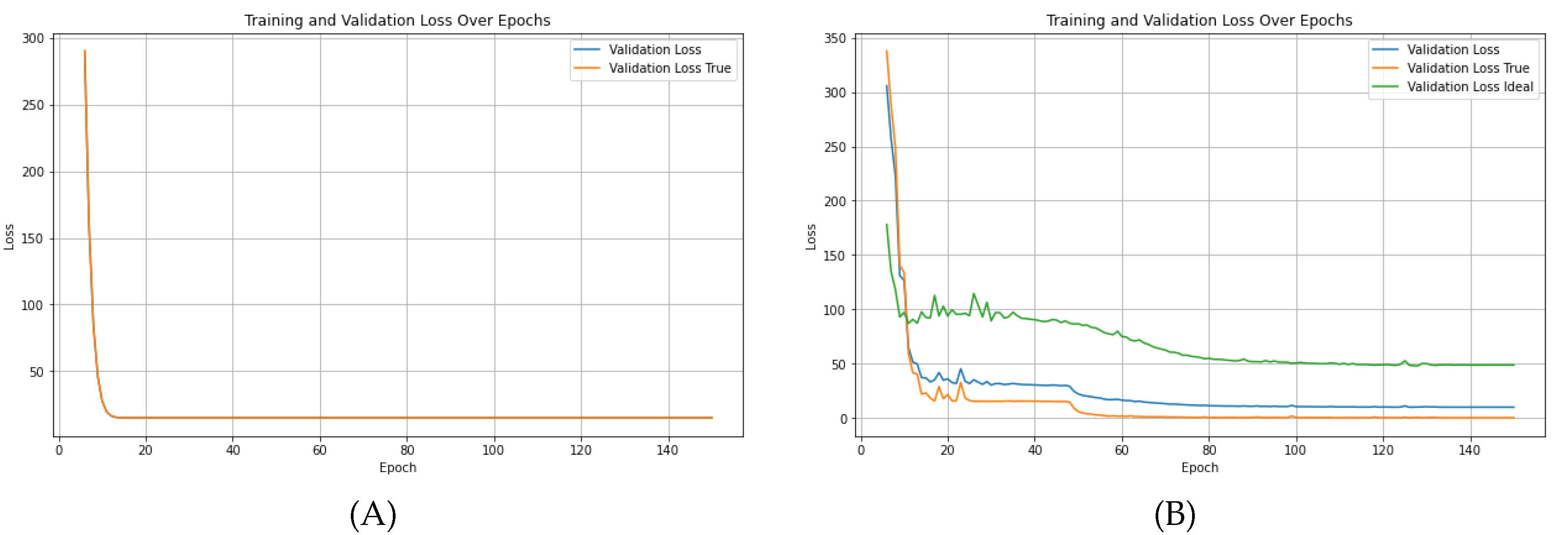
The network trained using only the MSE loss function initially showed a steady reduction in loss during the first few epochs. However, the loss quickly plateaued, indicating that the network struggled to minimize errors beyond a certain point. This plateau suggests that the MSE-only network fails to capture the complexities of seaweed growth over time fully.
In contrast, when training with the hybrid loss function, which combines MSE loss with physical loss (representing ideal growth rates based on physical laws), the network’s loss continued to decrease consistently over a longer training duration. This extended training time is compensated by the hybrid network’s ability to generalize better, achieving a significantly lower final loss than the MSE-only network. Figure 7 illustrates this behavior, where (A) shows the MSE-only loss reaching a plateau, and (B) demonstrates the continuous improvement of the hybrid network as it incorporates both real and ideal growth patterns.
4.1.2. Predicting Validation Accuracy
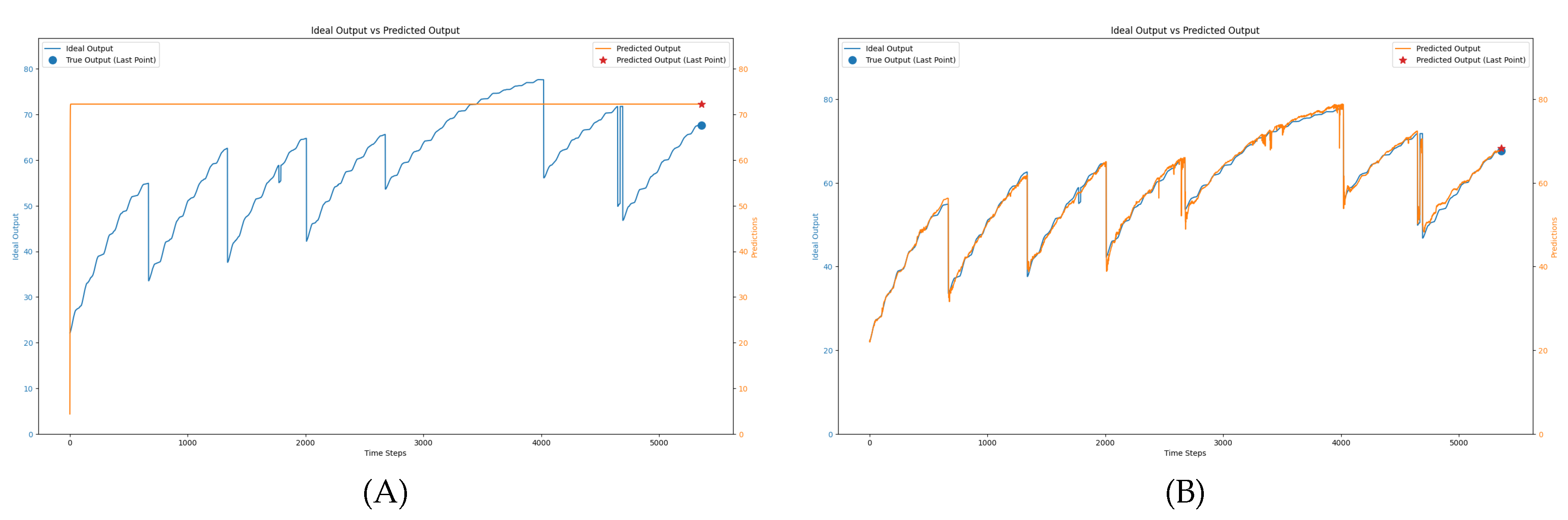
The network’s performance was further evaluated on the validation set, and the results indicate that the hybrid loss function significantly improves predictive accuracy. Two different loss functions were tested individually before combining them. Figure 8 compares the predictions of the LSTM model trained using only MSE loss (A) with the network trained using a hypothetical history of data points at every time step (B). In the case of the MSE-only network (A), the predictions are less accurate, as the network does not account for the underlying physical growth processes and instead relies solely on the final harvest data, leading to less accurate predictions. In contrast, the network trained with hypothetical data at every time step (B) shows overfitting to the data points generated from theoretical calculations, resulting in predictions that closely follow the ideal growth rate but do not account for real-world variations, making it too rigid and unsuitable for practical application.
Additionally, we evaluated the network’s performance using a simulated dataset where the seaweed weight data was available at different intervals, specifically every one day and every three days. When algae weight data is available daily, the traditional data-driven LSTM approach (using only the MSE loss function) maintains strong predictive accuracy, as it benefits from sufficient data points to learn from. However, as the frequency of available algae weight data decreases—such as every three days—the performance of the LSTM model trained solely with MSE begins to decline. The predictions become less aligned with the actual growth patterns due to the reduced number of ground truth data points. Despite this, the LSTM model continues to demonstrate robust performance by leveraging sequential data from other environmental inputs, such as temperature, humidity, and solar radiation.
To address these issues, a hybrid loss function was introduced, combining both MSE loss and physics constraint loss to balance real-world sensor data with theoretical growth networks. The hybrid approach allows the network to learn from empirical data while still respecting physical growth patterns, providing more reliable predictions that generalize better across different growth scenarios. Figure 10 illustrates how the hybrid loss function enables the network to produce significantly more accurate predictions, closely aligning with actual seaweed growth rates over time. This combination prevents overfitting to either the sensor noise or the theoretical network alone, leading to more balanced predictions.
It is important to note that during validation, certain sections in the ideal data points generated by the theoretical model showed unexpectedly low growth. Upon further investigation, it was found that these anomalies were associated with specific environmental conditions, such as abnormally high humidity or unusually low solar radiation. These environmental factors caused the theoretical model to deviate from expected growth patterns, highlighting the importance of accounting for such real-world variations when using purely physics-based constraints. The hybrid network’s ability to adapt to these anomalies while maintaining overall accuracy further underscores its robustness and applicability in real-world aquaculture systems.
4.2. Test Set Performance with Real Data
After training the LSTM model using generated data, the network was evaluated on real-world data to assess its performance in predicting actual seaweed growth rates. The test set consists of six datasets collected from three different sensors, allowing for a comprehensive evaluation of the network’s predictive accuracy.
4.2.1. Training with Non-Preprocessed Data
Table 1 shows the error results for the test data without any preprocessing (i.e., no moving average applied to the sensor values). Each LSTM model was trained using a hybrid loss function with different values of . The parameter in the hybrid loss function controls the balance between the sensor data (MSE loss) and the physical growth laws (physical loss). For example, LSTM () places more emphasis on the sensor data, while LSTM () gives equal importance to both the sensor data and the physical growth laws.
The table demonstrates how sensor noise can significantly impact network performance, especially when the hybrid loss function is skewed towards emphasizing the sensor data (e.g., ). LSTM with provides the best balance between sensor data and physical growth laws, resulting in the lowest prediction error. Interestingly, the network with shows a higher error, indicating that reducing the weight of the sensor data too much can cause the network to rely excessively on physical laws, leading to less accurate predictions.
4.2.2. Training with Preprocessed Data (Moving Average)
Table 2 presents the error results after applying a 6-hour moving average to the sensor data (preprocessed). The moving average helps smooth out fluctuations, allowing the network to make more accurate predictions by reducing the impact of sensor noise.
The preprocessed data, with the application of the 6-hour moving average, significantly improves prediction accuracy, especially for the hybrid network with . This network best captures both real-world sensor data and the physical growth patterns. For , the error is slightly higher, suggesting that while this weighting provides reasonable predictions, it still over-emphasizes physical laws.
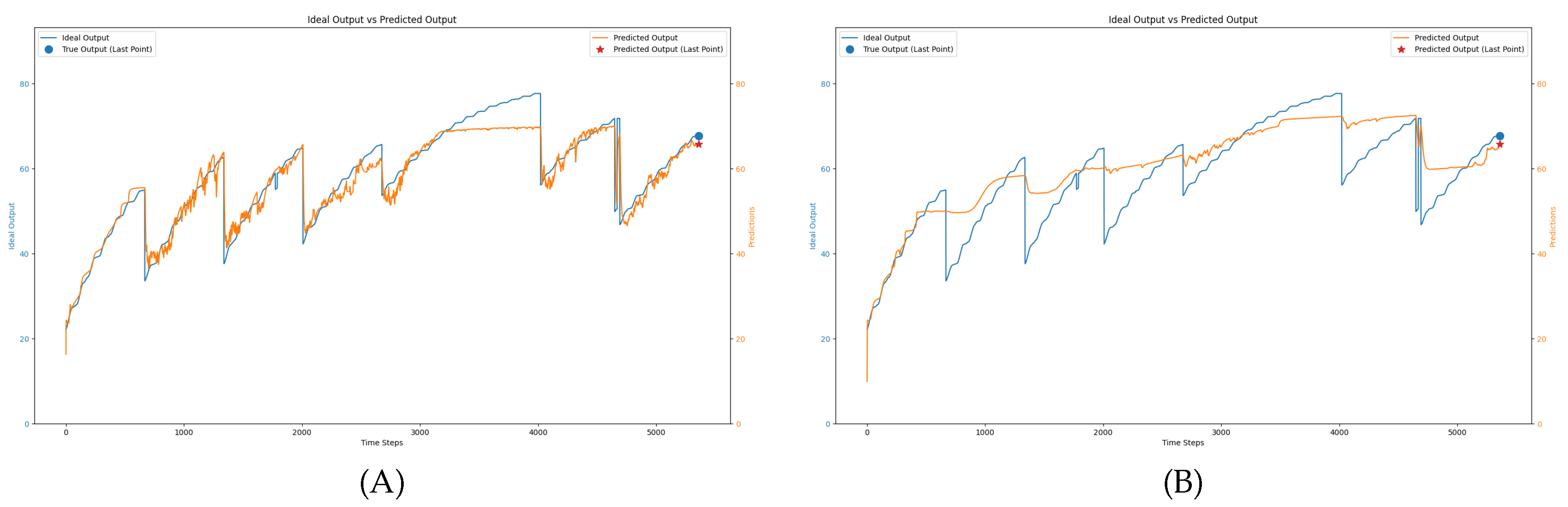
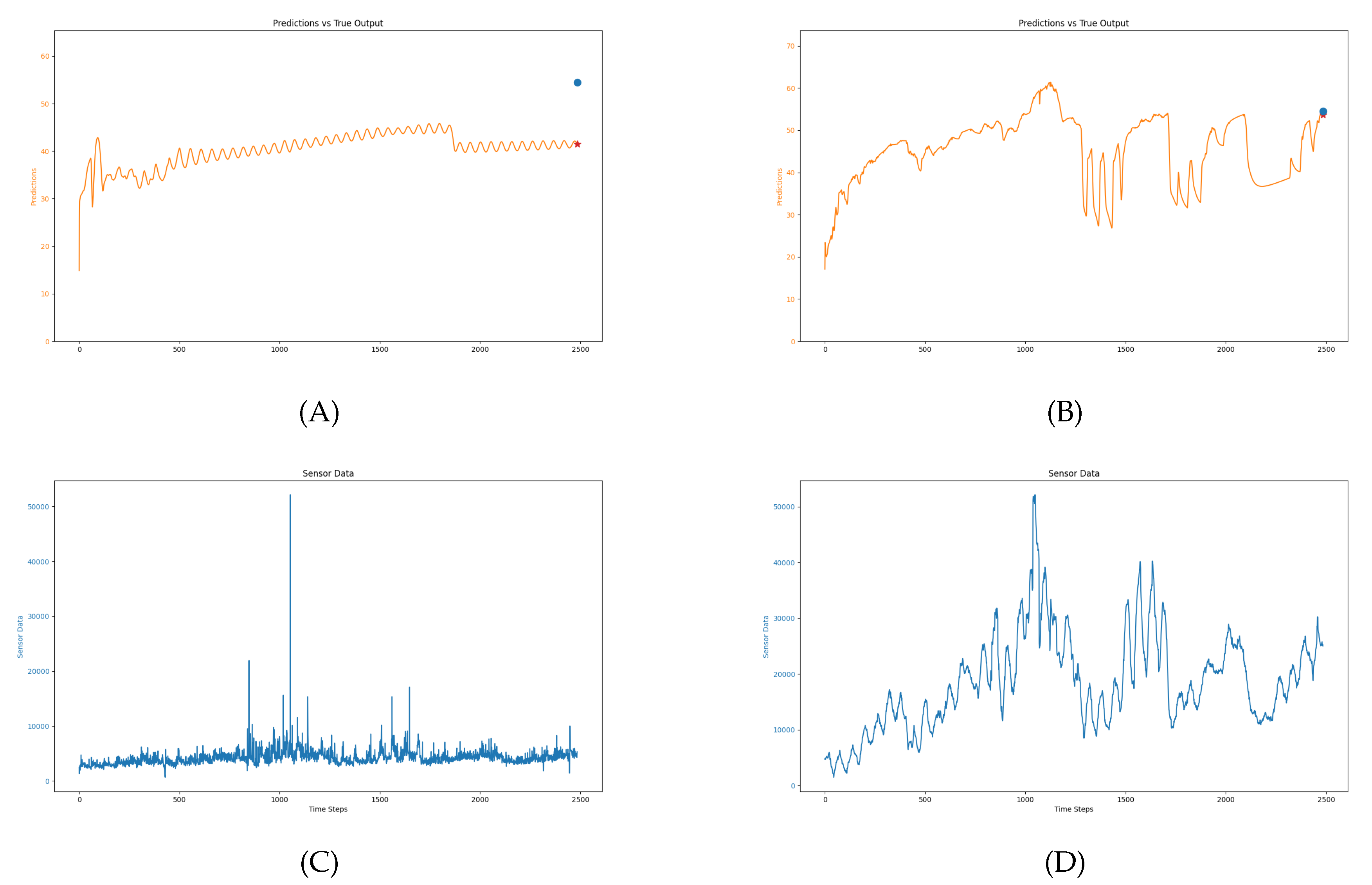
Figure 11 provides a visual comparison of seaweed growth predictions from sensor 5 using the same dataset. In Figure 11(A), the prediction reflects the day-to-day fluctuations in seaweed growth but fails to closely track the actual sensor values, as shown in Figure 11(C). These high variations confuse the network, preventing it from accurately correlating sensor readings with seaweed growth. In contrast, Figure 11(B) shows predictions that follow the sensor values more closely, after applying a 6-hour moving average, with the corresponding sensor values shown in Figure 11(D). The moving average reduces the impact of extreme variations, allowing the network to interpret the sensor data more effectively and predict seaweed growth more accurately. Preprocessing techniques such as moving averages significantly enhance prediction performance by mitigating the effects of noisy sensor data.
4.3. Effect of Varying in Hybrid Loss Function
Experiments with different values of in the hybrid loss function (, , , , ) revealed the importance of balancing the influence of sensor data and physical growth laws. When , the network overfit the physical growth patterns, resulting in lower accuracy when applied to real-world sensor data. The network relied too heavily on the theoretical physical constraints, ignoring sensor measurements that could reflect real-time variations and unexpected conditions in the environment.
On the other hand, with , the network overfit to sensor noise, diminishing the physical loss’s contribution to guiding the predictions. This led to predictions that closely followed the noisy sensor data but deviated from the expected growth patterns based on the laws of seaweed growth.
For , the network showed moderate improvements compared to , slightly reducing the overfitting to sensor noise. However, the prediction accuracy was still suboptimal compared to , where the network achieved the best balance between capturing real sensor measurements and adhering to the ideal growth dynamics provided by the physical laws.
Interestingly, the results for indicated that while the network still adhered well to physical growth laws, it began to place too little emphasis on sensor data, causing higher errors in scenarios where external environmental factors such as humidity and solar radiation significantly affected growth. The network was overly constrained by the idealized growth patterns, leading to less flexibility in adapting to the variations observed in real-world conditions.
Thus, the best performance was observed with , as this value offered the most balanced trade-off between sensor data and physical growth patterns, providing better predictive performance for real-world seaweed growth. This balance allowed the network to generalize well to unseen data while maintaining the theoretical understanding of seaweed growth, making it the most reliable choice for aquaculture prediction.
4.4. Relationship between Input Variables and Predicted Growth Rate
We examine the relationship between the input variables and the predicted seaweed growth rate. The purpose of this analysis is to illustrate how each environmental and sensor variable contributes to the prediction results, while also assessing the influence of preprocessing techniques such as applying a six-hour moving average to the sensor values.
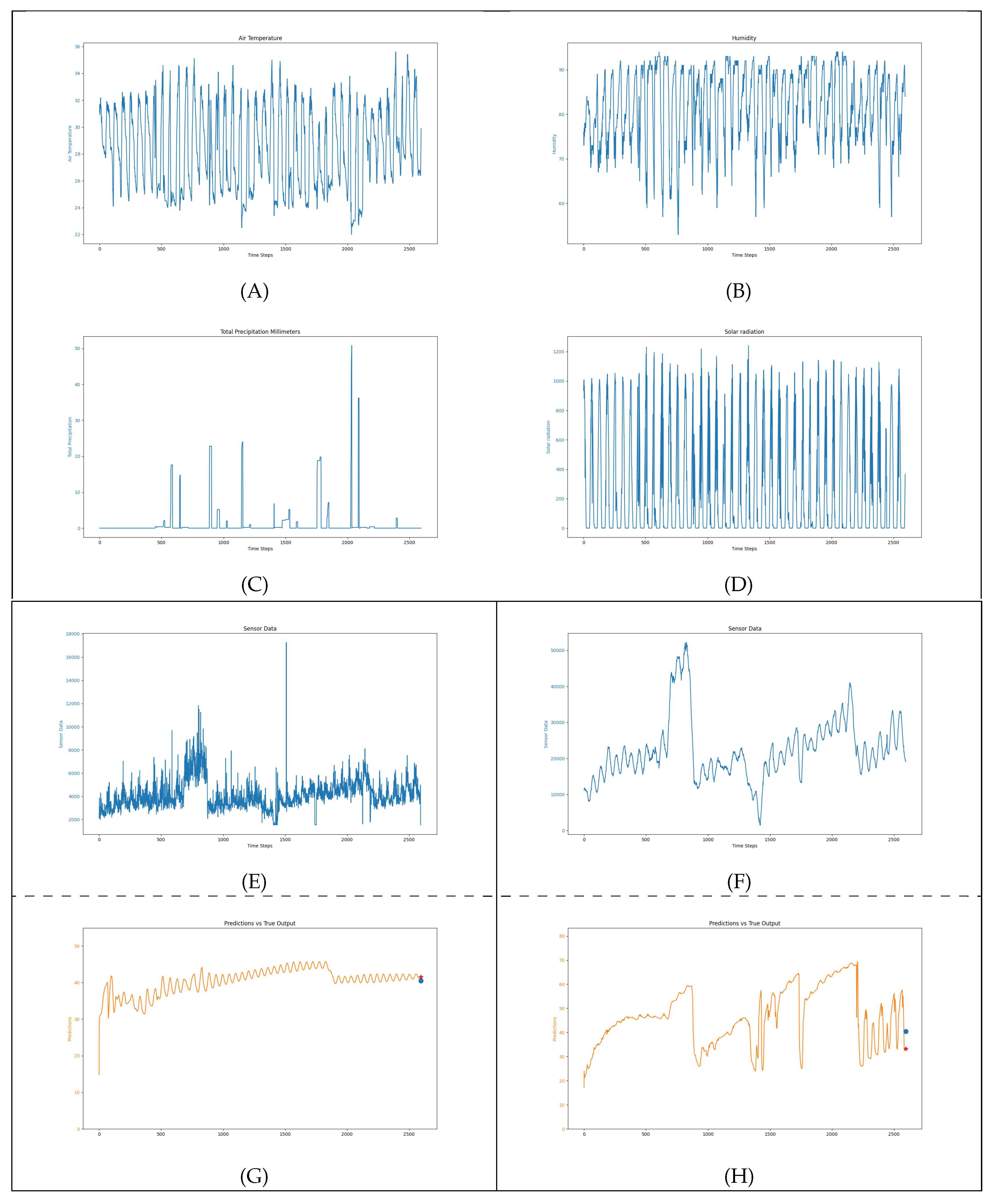
The input variables used in this model consist of both sensor data and environmental factors. These variables were collected in real time and play a significant role in determining the seaweed growth rates predicted by the LSTM model. The seven key input variables are visualized in Figure 12(A, B, C, D, E, F), which includes:
- Air Temperature (A): Seaweed growth is influenced by temperature variations, which can affect the metabolic rates of seaweed.
- Humidity (B): High humidity levels can impact evaporation rates and indirectly affect the water quality in the aquaculture tanks.
- Precipitation Intensity (C): These variables are related to rainfall events, which can introduce changes in water quality and temperature, indirectly affecting growth.
- Solar Radiation (D): Solar radiation provides the energy required for photosynthesis, a critical factor for seaweed growth.
- Sensor Values: The raw sensor values (Figure 12 E) capture high-frequency variations in seaweed growth, particularly in response to daily changes in environmental conditions, such as daylight and nighttime cycles. When a 6-hour moving average is applied (Figure 12 F), the fluctuations are smoothed out, reducing noise and improving the consistency of predictions.
The output predictions, shown in Figure 12(G, H), compare the results from using raw sensor data (without preprocessing) and sensor data with a 6-hour moving average:
- Without preprocessing (G): The predicted growth rate follows the sensor values closely, but high-frequency noise can cause deviations. In some cases, sensor fluctuations do not fully align with the expected growth pattern, leading to less accurate predictions.
- With 6-hour moving average (H): By smoothing the sensor data, the network can generate more stable and accurate predictions that better reflect the underlying growth rate. This is especially useful in filtering out the noise from daily fluctuations, enabling the network to focus on longer-term trends in seaweed growth.
The network’s predictions are primarily influenced by sensor values, which track high-frequency variations associated with seaweed growth. These variations are particularly evident during periods of high and low solar radiation, corresponding to the day-night cycle. However, predictions do not always strictly follow the sensor values. Upon further investigation, discrepancies often occur due to external weather conditions, such as heavy rainfall, which are captured by the Precipitation Intensity and Total Precipitation variables. These events can temporarily alter the growth conditions, leading to deviations in the predicted growth rate.
Moreover, our analysis revealed a consistent pattern of reduced predicted growth during periods of increased rainfall. While the precipitation data clearly impacts the model’s predictions, the degree to which the growth rate decreases is not fully interpretable due to the "black box" nature of the neural network. This challenge is typical of deep learning models, where it can be difficult to understand the exact contribution of each input variable to the final prediction. Nonetheless, precipitation consistently appears to lower predicted growth, although the precise magnitude of this reduction remains unclear.
4.5. Harvesting Decision Support
An interesting observation in Figure 12 (B) is the noticeable decline in seaweed growth rates during certain periods, resulting in a reduction of the overall seaweed biomass. This could be attributed to several factors, such as the saturation of seaweed in the tank or a deterioration in water quality. Such drops in growth rates may indicate that the seaweed has reached a point of diminishing returns in terms of biomass growth, or that environmental conditions in the tank are no longer optimal for sustained growth.
4.6. Comparison with Previous Algorithm
This study extends upon previous research, which utilized Polynomial Regression and RANSAC to predict final seaweed mass. Polynomial regression relies solely on the current data point and previous points to make predictions. However, if data is missing or there is a sudden error, the prediction accuracy is immediately compromised. Even with RANSAC and moving average applied to reduce noise, these methods fail to handle such issues effectively.
In contrast, the LSTM model follows the timeline of the data, using sequential information and incorporating a forget gate mechanism. This allows the network to filter out irrelevant data and learn which parts of the data should or should not be used. The LSTM’s performance improves significantly when noise is reduced using a moving average, as it can focus on the true growth patterns more effectively.
The comparison between these older methods and the proposed LSTM model with hybrid loss is shown in Table 3.
The results clearly demonstrate that the LSTM model with hybrid loss provides significantly better predictions than the traditional regression methods, even though it was not trained on real data.
5. Discussion
One of the key considerations in this study is the choice of variables used for network training. Although the nutrient levels, solar irradiance, and water temperature directly influence seaweed growth, these variables are not always feasible for continuous real-time measurement in large-scale aquaculture systems. Therefore, the environmental factors—solar radiation, rainfall, and air temperature—were incorporated into the network. These factors, although not direct indicators of seaweed growth, provide a practical solution for real-time prediction due to their availability through environmental sensors. This approach allows the network to leverage real-time data, ensuring that predictions remain timely and relevant for practical aquaculture applications.
Using LSTM with generated data yielded better results compared to using regression alone. However, training with generated data alone poses significant risks, especially if environmental conditions or seaweed species change. To improve network performance, it is recommended to fine-tune the pretrained model on real data before applying it in practice. Additionally, replacing LSTM with networks like GPT could enhance learning performance further [12].
Another critical challenge with sensor data is to mitigate noise. In many cases, the sensor data exhibits large and unpredictable variations, or at times, the readings show extreme spikes or remain stagnant for long periods. This may occur if a chunk of algae is stuck at the sensor viewport. These anomalies make it difficult to achieve accurate predictions, as the sensors should ideally respond only to changes in seaweed density. Such noise interferes with the network’s ability to interpret growth patterns correctly. Currently, We are improving the sensor design to address this issue.
In Figure 13, we present an example of sensor data where extreme noise is evident. The erratic behavior of the sensor readings, marked by significant spikes, demonstrates the challenge of maintaining prediction accuracy even with the use of preprocessing techniques like moving averages. Despite applying a six-hour moving average, the network’s predictions fail to follow the sensor closely due to the magnitude of the noise. This issue highlights the importance of addressing sensor anomalies to improve the reliability of seaweed growth predictions.
In fact, experiments with GPT-2 were conducted to improve the network for prediction, yielding promising results (see Figure 14). However, due to the complexity and time requirements for setting up and training GPT-based networks, they were not included in this study’s final comparison. We will discuss the results of this approach in a future manuscript.
An additional advantage of using LSTM for prediction is its ability to more accurately assess seaweed growth over both day and night cycles. Since LSTM incorporates data across the entire timeframe, including periods of solar radiation, it can better understand the true growth rate of the seaweed. In contrast, regression models tend to discard high levels of noise during daytime sensor readings, thereby missing out on valuable information and underestimating growth rates. The LSTM’s sequential learning mechanism, therefore, provides a more reliable representation of the seaweed growth process than regression methods, which are more limited in their ability to handle temporal dynamics effectively.
5.1. Application of Harvesting Decision Support
The LSTM model’s ability to detect fluctuations in growth rates offers a potential for real-time decision support in aquaculture. Notably, in some periods, as observed in Figure 12(B), the seaweed growth rate declines significantly, suggesting factors such as seaweed saturation or degraded water quality. These declines may indicate that the seaweed has reached a growth plateau, or that the environmental conditions are no longer optimal.
Leveraging this network, an automated system could monitor growth patterns and trigger alerts for timely harvesting before seaweed becomes too dense or growth rates stagnate. Additionally, the system could recommend water quality adjustments to optimize growth conditions. It’s important to note that the IMTA system is recirculating, with water turnover in the tanks occurring every other hour. Therefore, growth plateaus may not be directly related to water quality but could instead be due to density-dependent limitations, such as reduced light penetration caused by the high density of algae in the tank. Implementing such decision support systems could improve both the efficiency and sustainability of the IMTA system, ensuring timely interventions based on real-time data.
6. Conclusions
In this study, we developed a novel approach for predicting seaweed growth in Integrated Multi-Trophic Aquaculture (IMTA) systems by leveraging Long Short-Term Memory (LSTM) models with physical constraints. Our network integrates natural and synthetic data, incorporating key environmental factors such as air temperature, solar radiation, and nutrient levels to simulate realistic growth conditions. The proposed technique significantly improved the network’s predictive accuracy by adopting a hybrid loss function, combining traditional Mean Squared Error (MSE) with physical laws governing seaweed growth.
The results demonstrated that the LSTM model trained with hybrid loss outperformed networks trained with MSE alone and traditional regression methods like RANSAC, particularly in handling noisy sensor data. The hybrid loss function enabled the network to better understand the underlying physical process of seaweed growth, resulting in more accurate predictions across various environmental conditions. Furthermore, preprocessing techniques such as moving average were found to be essential in mitigating the effects of noise, further enhancing prediction reliability.
Experiments with different values of in the hybrid loss function revealed the importance of balancing sensor data and physical laws. The optimal performance was achieved with , where the network successfully integrated both sources of information to improve predictive performance.
Although the LSTM model showed promising results, issues remain. In particular, the limited availability of real-world data and the inherent noise in sensor readings pose significant challenges. One future endeavor will be to improve the sensor design, such as exploring different wavelengths of laser sources. We will also explore alternative architectures, such as GPT-based networks, that may offer superior performance in handling sequential data.
In conclusion, this research highlights the potential of combining machine learning with domain-specific physical knowledge to optimize seaweed growth in aquaculture systems. Beyond predictive accuracy, the network’s ability to support real-time harvesting decisions demonstrates its practical value. Integrating advanced predictive networks with sensor technology offers a pathway to more sustainable and efficient aquaculture practices, enabling real-time monitoring and decision-making for biomass management. Another essential drive of this research is that a similar methodology may be developed to provide reliable long-term prediction (i.e., > 24 hours) of dissolved oxygen levels in an aquaculture pond - a key component in the "Intelligent Resource Efficient Pond Aquaculture (IREPA)" project [40].
Author Contributions
Conceptualization, Bing Ouyang; methodology, Alisa Kunapinun and William Fairman; software, Alisa Kunapinun; validation, Paul S. Wills, Denis Hanisak, and Bing Ouyang; formal analysis, Alisa Kunapinun; investigation, Alisa Kunapinun; resources, William Fairman, Paul S. Wills, Denis Hanisak, and Bing Ouyang; data curation, William Fairman; writing—original draft preparation, Alisa Kunapinun; writing—review and editing, Bing Ouyang; visualization, Alisa Kunapinun; supervision, Bing Ouyang; project administration, Bing Ouyang; funding acquisition, Bing Ouyang. All authors have read and agreed to the published version of the manuscript.
Funding
This research was funded in part by the USDA-NIFA Grants 2019-67022-29204 and 2024-67022-41580, as well as the Aquaculture Specialty License Plate and the Save Our Sea Specialty License Plate funds granted through the Harbor Branch Oceanographic Institute Foundation.
Institutional Review Board Statement
Not applicable.
Informed Consent Statement
Not applicable.
Data Availability Statement
The data supporting the reported results, including scripts and partial generated datasets, can be found at: https://github.com/Alisa-Kunapinun/BiomassLSTM.
Acknowledgments
The authors would like to express their deepest gratitude to Denis Hanisak for his invaluable contributions to this work. His dedication and expertise greatly advanced the research, and his passing is a profound loss to the scientific community. This paper is dedicated to his memory.
Conflicts of Interest
The authors declare no conflicts of interest. The funders had no role in the design of the study; in the collection, analyses, or interpretation of data; in the writing of the manuscript; or in the decision to publish the results.
References
- Fairman W., Wills P. S., Hanisak D., & Ouyang B. (2022). Pseudorandom encoded-light for evaluating biomass (PEEB): a robust COTS macroalgal biomass sensor for the integrated multi-trophic aquaculture (IMTA) system. In Big Data IV: Learning, Analytics, and Applications (Vol. 12097, pp. 165-173).
- Fairman W., Wills P. S., Hanisak D., Karim A., Singh S., & Ouyang B. (2023). Deployment of the pseudorandom encoded light for evaluating biomass (PEEB) sensor in an integrated multi-trophic aquaculture (IMTA) system. In Big Data V: Learning, Analytics, and Applications (Vol. 12522, p. 1252204).
- Kunapinun Alisa, William Fairman, Paul S. Wills, Dennis Hanisak, Shagundeep Singh, and Bing Ouyang. "Quantifying sea lettuce density in an integrated multi-trophic aquaculture (IMTA) system: understanding the complex physical process through multi-modality data modeling." In Big Data VI: Learning, Analytics, and Applications, vol. 13036, pp. 68-80. SPIE, 2024.
- B. Ouyang et al., "Initial Development of the Hybrid Aerial Underwater Robotic System (HAUCS): Internet of Things (IoT) for Aquaculture Farms," in IEEE Internet of Things Journal, vol. 8, no. 18, pp. 14013-14027, 15 Sept.15, 2021. [CrossRef]
- Lora Alliance. What is LoRaWAN?; 2020. Available online: https://lora-alliance.org/wp-content/uploads/2020/11/what-is-lorawan.pdf (accessed on November 2015).
- Sener, O. , & Koltun V. (2018). Multi-task learning as multi-objective optimization. Advances in Neural Information Processing Systems, 31.
- Jayaraman, S. K. , & Rhinehart, R. R. (2015). Modeling and optimization of algae growth. Industrial & Engineering Chemistry Research, 54(33), 8063-8071.
- Ogle D. H., & Isermann D. A. (2017). Estimating age at a specified length from the von Bertalanffy growth function. North American Journal of Fisheries Management, 37(5), 1176-1180.
- Bengio, Y. , Simard P., & Frasconi P. (1994). Learning long-term dependencies with gradient descent is difficult. IEEE Transactions on Neural Networks, 5(2), 157-166.
- Hochreiter, S. , & Schmidhuber, J. (1997). Long short-term memory. Neural Computation, 9(8), 1735-1780.
- Graves, A. (2012). Supervised sequence labelling with recurrent neural networks (Vol. 385). Springer.
- Radford, A. , Narasimhan K., Salimans T., & Sutskever I. (2018). Improving language understanding by generative pre-training. OpenAI.
- Flunkert, V. , Salinas D., & Gasthaus J. (2017). DeepAR: Probabilistic forecasting with autoregressive recurrent networks. arXiv:1704.04110.
- Borovykh, A. , Bohte S., & Oosterlee C. W. (2017). Conditional time series forecasting with convolutional neural networks. arXiv:1703.04691.
- Lim, B. , Zohren S., & Roberts S. (2019). Temporal fusion transformers for interpretable multi-horizon time series forecasting. arXiv:1912.09363.
- Raissi, M. , Perdikaris P., & Karniadakis G. E. Physics-informed neural networks: A deep learning framework for solving forward and inverse problems involving nonlinear partial differential equations. Journal of Computational Physics, 2019; 378, 686–707. [Google Scholar]
- Lutter, M. , Ritter C., & Peters J. (2019). Deep Lagrangian networks: Using physics as model prior for deep learning. arXiv:1907.04490.
- Omer Faruk, D. (2010). A hybrid neural network and ARIMA model for water quality time series prediction. *Engineering Applications of Artificial Intelligence*, 23(4), 586–594.
- Bai, Y.-T. , Su, T.-L., & Kong, J.-L. (2020). Hybrid Deep Learning Predictor for Smart Agriculture Sensing Based on Empirical Mode Decomposition and Gated Recurrent Unit Group Model. *Sensors*, 20(5), 1334.
- Ojo, M. O., & Zahid, A. (2022). Deep Learning in Controlled Environment Agriculture: A Review of Recent Advancements, Challenges, and Prospects. *Sensors*, 22(20), 7965.
- Nordin, R., Gharghan, S. K., Jawad, A. M., & Ismail, M. (2017). Energy-Efficient Wireless Sensor Networks for Precision Agriculture: A Review. *Sensors*, 17(8), 1781.
- Kalman, R. E. A new approach to linear filtering and prediction problems. Journal of Basic Engineering, 1960; 82, 35–45. [Google Scholar]
- Welch, G. , & Bishop, G. (1995). An Introduction to the Kalman Filter. Technical Report TR 95-041, University of North Carolina at Chapel Hill.
- Gers F., A. , Schraudolph N. N., & Schmidhuber J. (2002). Learning precise timing with LSTM recurrent networks. Journal of Machine Learning Research, 3, 115–143.
- Graves, A. , & Schmidhuber J. (2005). Framewise phoneme classification with bidirectional LSTM and other neural network architectures. Neural Networks, 18, 602–610.
- Lipton Z., C. , Berkowitz J., & Elkan C. (2015). A critical review of recurrent neural networks for sequence learning. arXiv preprint arXiv:1506.00019, arXiv:1506.00019.
- Kalchbrenner, N. , & Blunsom P. (2013). Recurrent continuous translation models. In Proceedings of the 2013 Conference on Empirical Methods in Natural Language Processing (pp. 1700-1709). [Google Scholar]
- Graves, A. , Mohamed A. R., & Hinton G. (2013). Speech recognition with deep recurrent neural networks. In 2013 IEEE International Conference on Acoustics, Speech and Signal Processing (pp. 6645-6649).
- Rangapuram S., S. , Seeger M., Gasthaus J., Stella L., Wang Y., & Januschowski T. (2018). Deep state space models for time series forecasting. In Advances in Neural Information Processing Systems (pp. 7785-7794).
- Hewamalage, H. , Bergmeir C., & Bandara K. (2021). Recurrent neural networks for time series forecasting: Current status and future directions. International Journal of Forecasting, 2021; 37, 388–427. [Google Scholar]
- Bandara, K. , Shi P., & Bergmeir C. (2020). Sales demand forecasting with forecast combinations of temporal hierarchical reconciliation and machine learning. European Journal of Operational Research. 281, 327–342.
- Smyl, S. (2020). A hybrid method of exponential smoothing and recurrent neural networks for time series forecasting. International Journal of Forecasting, 2020; 36, 75–85. [Google Scholar]
- Shih, S. , Sun F. Y., & Lee H. H. (2019). Temporal pattern attention for multivariate time series forecasting. In Advances in Neural Information Processing Systems (pp. 10470-10480).
- Hara, K. , & Hida S. (2018). Forecasting stock prices with attention-based neural networks. arXiv:1806.03589.
- Verma, S. (2021). A Comparative Study of Time Series Models for Forecasting Aquaculture Environmental Parameters. Environmental Science and Pollution Research, 28(10), 12891–12905.
- Qi, Z., et al. (2019). Predicting water quality time series using deep learning models with empirical models for aquaculture monitoring. Journal of Hydroinformatics. 21(4), 654–666.
- Lai, X., & Zeng, S. (2019). A Hybrid Deep Learning Model for Aquaculture Growth Prediction Combining LSTM and Domain Knowledge. Aquaculture Reports, 13, 100204.
- Sun, Z. , et al. (2021). Time Series Forecasting of Fish Growth in Recirculating Aquaculture Systems Using LSTM and Data Augmentation Techniques.Computers and Electronics in Agriculture. 2021, 184, 106139. [Google Scholar]
- M. Levy and J. O. Hallstrom, "A new approach to data center infrastructure monitoring and management (DCIMM)," 2017 IEEE 7th Annual Computing and Communication Workshop and Conference (CCWC), Las Vegas, NV, USA, 2017, pp. 1-6. [CrossRef]
- Bing Ouyang, Paul S. Wills, Yufei Tang, Tsung-Chow Su and James Garvey, "Intelligent Resource Efficient Pond Aquaculture (IREPA): Cyber-Physical System to Improve the Fish Farms Productivity in the U.S.," NSF 2024 Cyber-Physical Systems (CPS) Principal Investigators’ Meeting, March 2024.
| 1 | For a detailed explanation of the Kalman filter, including the prediction and update equations, refer to [23]. |
Figure 1.
An overview of the IMTA IoT framework and the layout of the HBOI Aquaculture Research Facility, paving the way for an in-depth discussion of the next-generation biomass sensor and its crucial role in enhancing aquaculture analytics. Reprinted from [Fairman2022].
Figure 1.
An overview of the IMTA IoT framework and the layout of the HBOI Aquaculture Research Facility, paving the way for an in-depth discussion of the next-generation biomass sensor and its crucial role in enhancing aquaculture analytics. Reprinted from [Fairman2022].
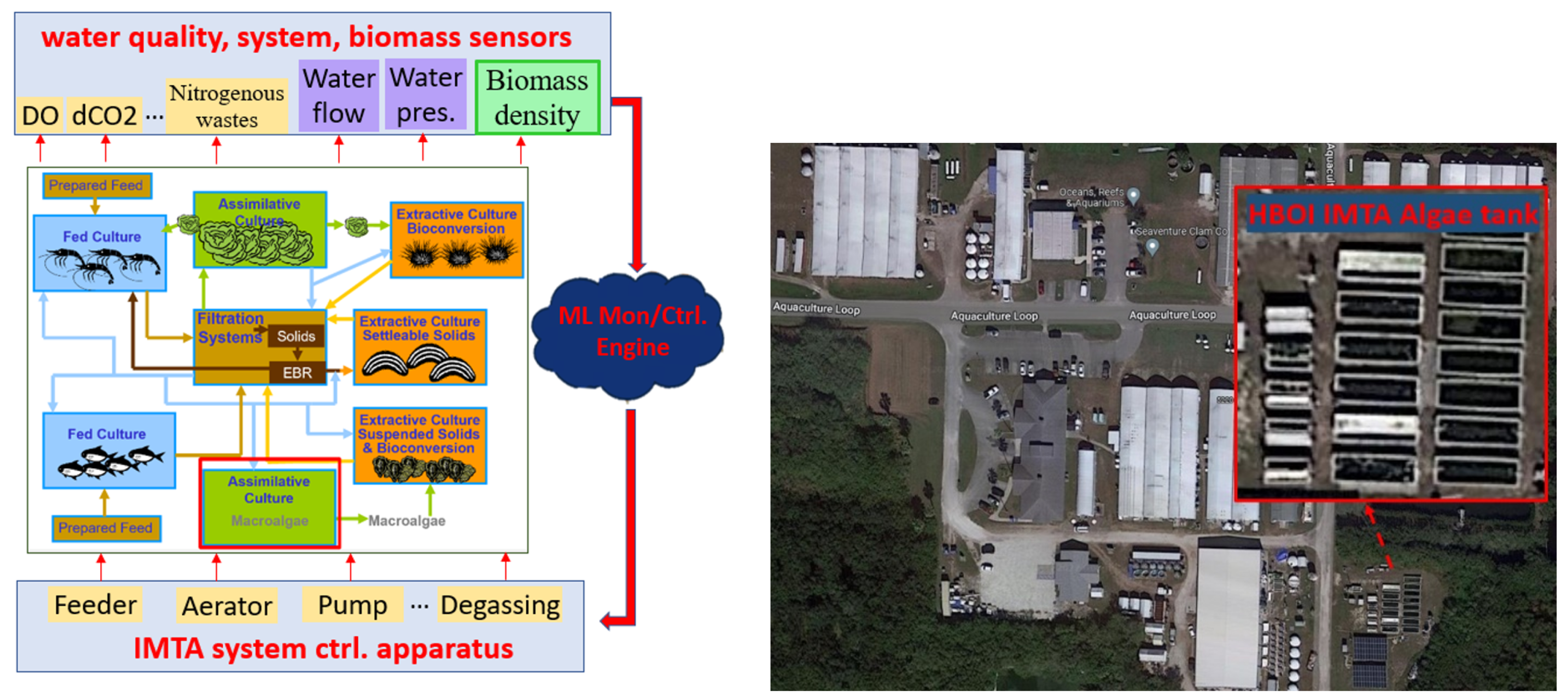
Figure 2.
The use of sensors and their installation in the seaweed cultivation tank. (A) illustrates the configuration and installation of the sensor, (B) illustrates the water tank layout, and the sensor positions in the seaweed cultivation tank. Reprint from [Kunapinun2024]
Figure 2.
The use of sensors and their installation in the seaweed cultivation tank. (A) illustrates the configuration and installation of the sensor, (B) illustrates the water tank layout, and the sensor positions in the seaweed cultivation tank. Reprint from [Kunapinun2024]
| (A) |
| (B) |
Figure 3.
Simulated seaweed growth rate over an eight-week cultivation period, incorporating tank dimensions, initial biomass, and environmental conditions. The model includes weekly harvests with variable weights and integrates real-time solar irradiance data from weather sensors. The growth rate reflects biomass changes under both optimal and varying environmental factors, simulating the conditions in the IMTA system.
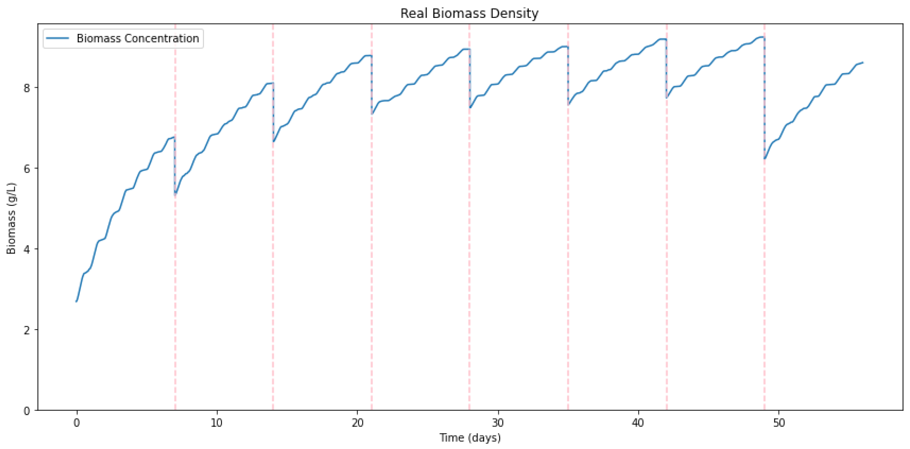
Figure 4.
Generated sensor data reflecting seaweed growth rates with added noise for realism. The sensor readings, derived from simulated growth rates, account for IR sensor sensitivity to seaweed density. The conversion equation applied integrates the average calibration factor and minimum sensor reading, ensuring the generated data mimics actual sensor output in the IMTA system.
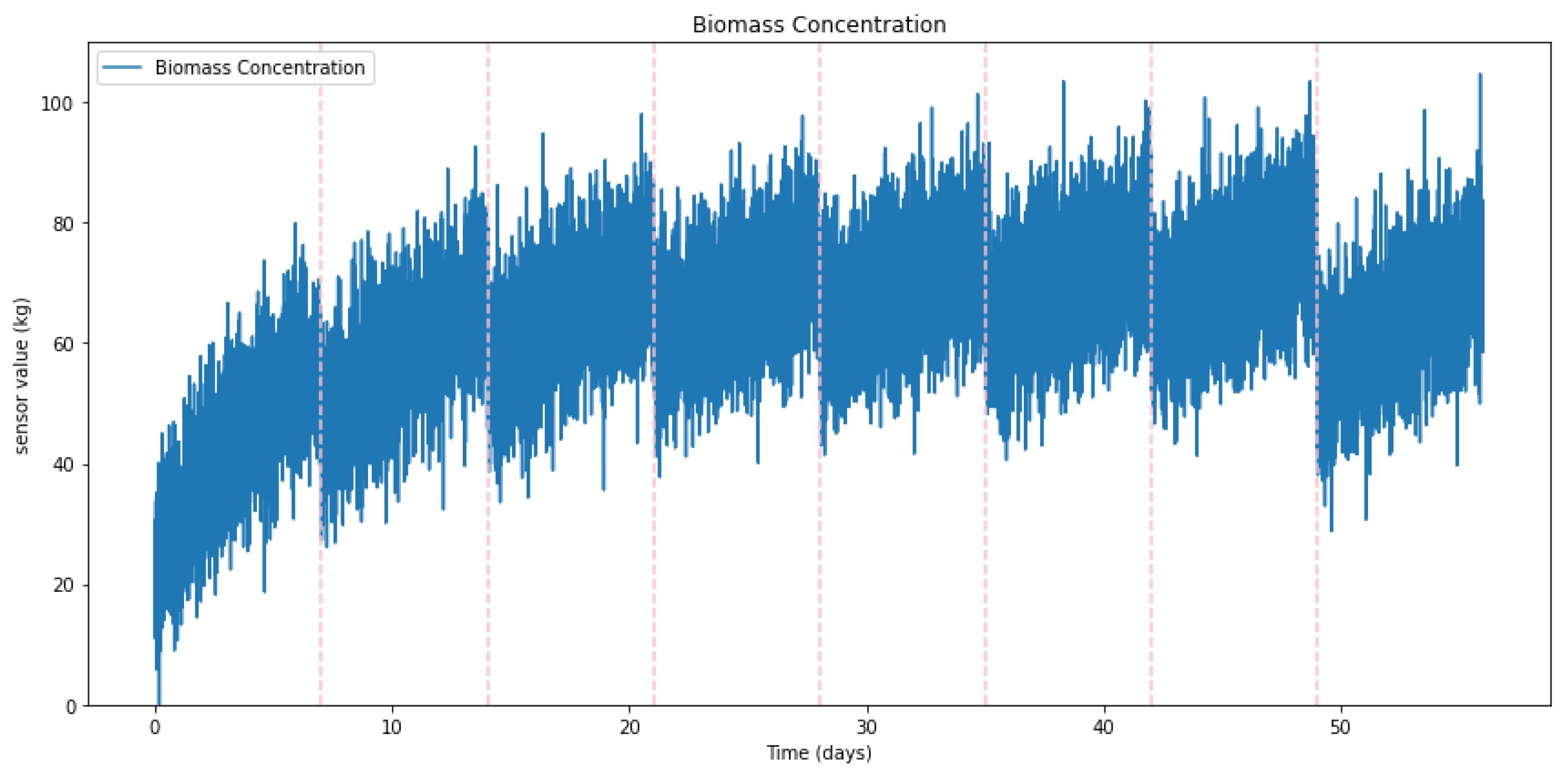
Figure 5.
Schematic representation of the LSTM model architecture used for predicting seaweed mass in the tank, with 5 hidden layers and various input features like solar radiation, air temperature, and sensor values.
Figure 5.
Schematic representation of the LSTM model architecture used for predicting seaweed mass in the tank, with 5 hidden layers and various input features like solar radiation, air temperature, and sensor values.

Figure 6.
The architecture of the LSTM model incorporates the hybrid loss function, which combines physical loss and MSE loss. : Ideal weight of seaweed at each time step, : Predicted weight at each time step, : Ground truth weight at the final time step, and : Predicted weight at the final time step.
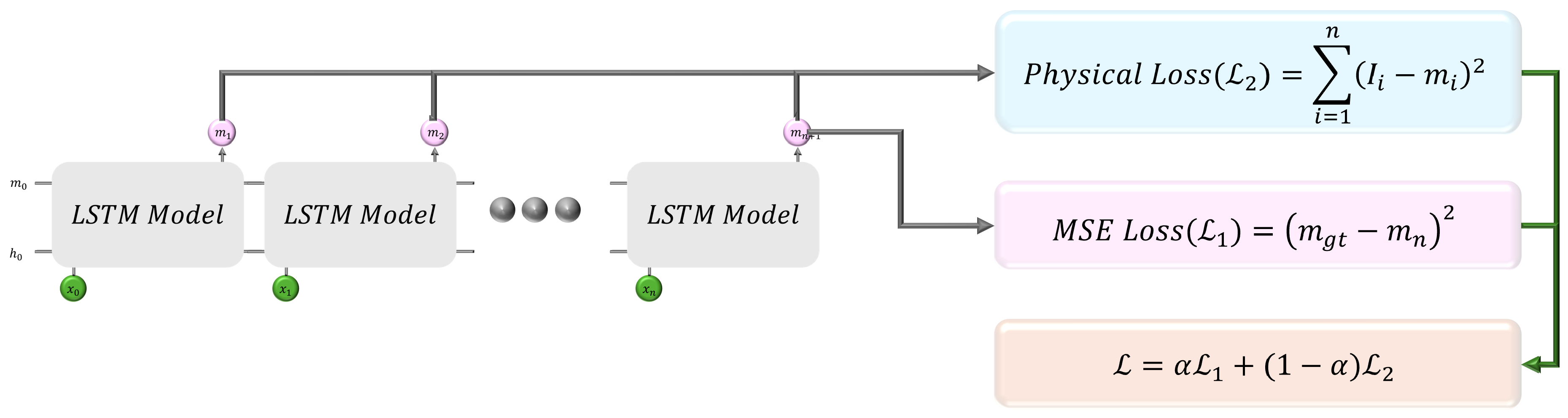
Figure 7.
Training loss over 150 epochs: (A) The network trained with only MSE loss plateaus around 15, showing limited further improvement. (B) The network trained with hybrid loss (80% MSE, 20% physical loss) exhibits continuous improvement, better capturing the temporal dynamics of seaweed growth.
| (A) | (B) |
Figure 8.
Comparison of seaweed growth prediction results: (A) Network trained with only MSE loss, where the prediction fails to follow the growth trends throughout the cultivation period, relying solely on final data points. (B) Network trained with a hypothetical history of data at every time step, leading to overfitting, as the predictions strictly adhere to growth patterns without accounting for real-world sensor data.
| (A) | (B) |
Figure 9.
Seaweed growth prediction with varying frequencies of algae weight data availability: (A) Predictions with daily data, (B) Predictions with data available every three days. As the data becomes less frequent, the predictive accuracy declines; however, the LSTM model still preserves a reasonable level of performance by utilizing sequential data from other environmental factors.
| (A) | (B) |
Figure 10.
Seaweed growth prediction using the hybrid loss function, which combines MSE loss and physics constraint loss. The hybrid network shows significantly more accurate predictions aligned with actual growth data, avoiding both overfitting and underfitting by balancing real-world sensor data with theoretical growth networks.
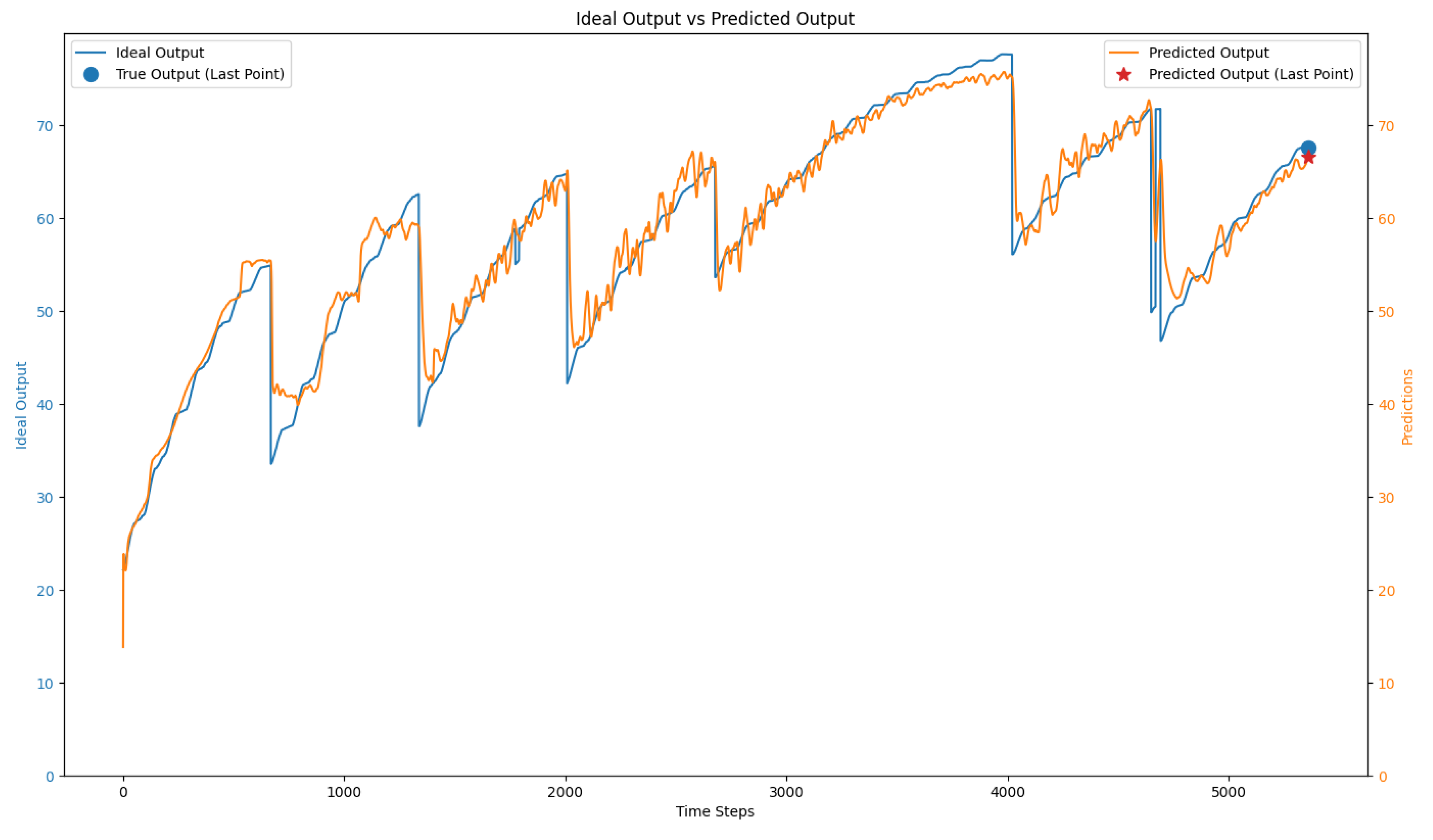
Figure 11.
Seaweed growth prediction with sensor values (Sensor 5): (A) Seaweed growth prediction without applying a moving average, (B) Seaweed growth prediction with a 6-hour moving average. (C) Sensor values without applying a moving average, (D) Sensor values with a 6-hour moving average.
Figure 11.
Seaweed growth prediction with sensor values (Sensor 5): (A) Seaweed growth prediction without applying a moving average, (B) Seaweed growth prediction with a 6-hour moving average. (C) Sensor values without applying a moving average, (D) Sensor values with a 6-hour moving average.
| (A) | (B) |
| (C) | (D) |
Figure 12.
Input variables used for prediction: (A) Air temperature, (B) Humidity, (C) Precipitation intensity, (D) Solar radiation, (E) Sensor values without preprocessing, (F) Sensor values with a 6-hour moving average. Predicted seaweed growth rate: (G) Prediction using raw sensor data (without preprocessing), and (H) Prediction using sensor data with a 6-hour moving average.
| (A) | (B) |
| (C) | (D) |
| (E) | (F) |
| (G) | (H) |
Figure 13.
An example of sensor data with significant noise. The large spikes and erratic behavior in the sensor readings hinder accurate seaweed growth predictions, even with preprocessing methods such as moving averages.
Figure 13.
An example of sensor data with significant noise. The large spikes and erratic behavior in the sensor readings hinder accurate seaweed growth predictions, even with preprocessing methods such as moving averages.
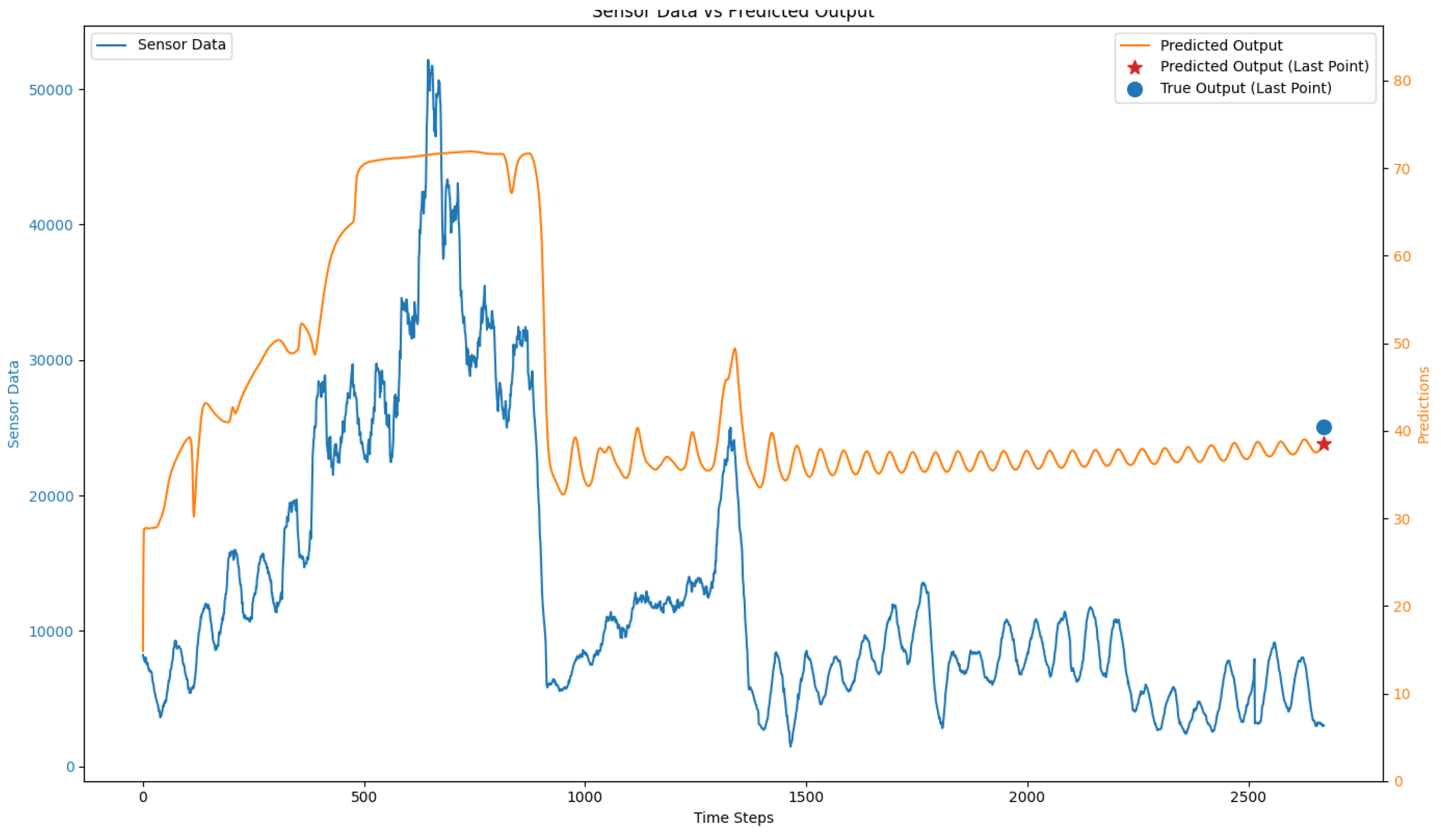
Figure 14.
GPT-2 result after training with dummy data without noise.
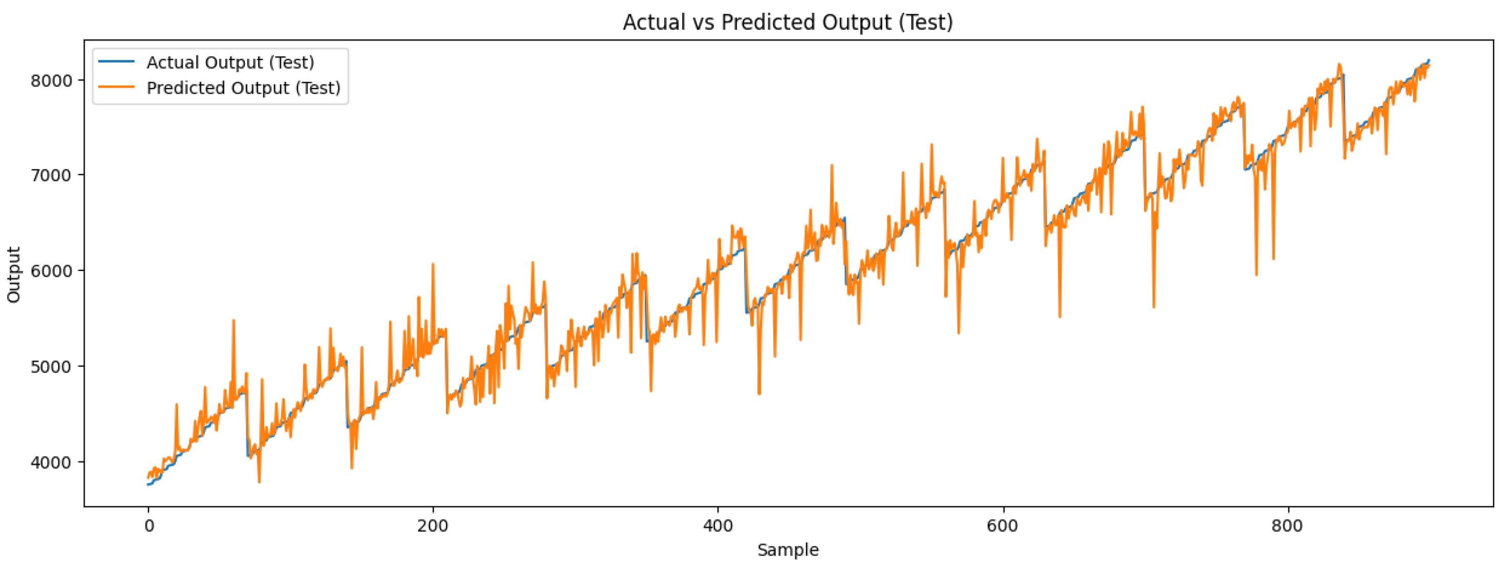

Table 1.
Error results on non-preprocessed sensor data
| Sensor No | Ideal | LSTM | LSTM | LSTM | LSTM | LSTM |
|---|---|---|---|---|---|---|
| Calculation | () | () | () | () | () | |
| 1 | 20.59 | 30.17 | 7.34 | 6.54 | 15.18 | 31.86 |
| 4 | 20.59 | 30.32 | 6.98 | 6.63 | 12.50 | 32.17 |
| 5 | 20.59 | 30.81 | 7.33 | 6.99 | 19.28 | 31.20 |
| All | 20.59 | 30.43 | 7.21 | 6.71 | 15.65 | 31.75 |
Table 2.
Error results on preprocessed sensor data (6-hour moving average)
| Sensor No | Ideal | LSTM | LSTM | LSTM | LSTM | LSTM |
|---|---|---|---|---|---|---|
| Calculation | () | () | () | () | () | |
| 1 | 20.59 | 19.53 | 7.49 | 8.18 | 12.61 | 31.78 |
| 4 | 20.59 | 15.25 | 17.28 | 7.92 | 8.04 | 28.72 |
| 5 | 20.59 | 4.02 | 3.79 | 7.85 | 6.66 | 30.10 |
| All | 20.59 | 12.94 | 9.52 | 7.98 | 9.10 | 30.20 |
Table 3.
Comparison of Average Prediction Error
| Algorithm | Average Error (kg) |
|---|---|
| Polynomial Regression | 14.09 |
| LSTM (, no preprocessing) | 6.72 |
| LSTM (, with moving average) | 7.98 |
Disclaimer/Publisher’s Note: The statements, opinions and data contained in all publications are solely those of the individual author(s) and contributor(s) and not of MDPI and/or the editor(s). MDPI and/or the editor(s) disclaim responsibility for any injury to people or property resulting from any ideas, methods, instructions or products referred to in the content. |
© 2024 by the authors. Licensee MDPI, Basel, Switzerland. This article is an open access article distributed under the terms and conditions of the Creative Commons Attribution (CC BY) license (http://creativecommons.org/licenses/by/4.0/).
Copyright: This open access article is published under a Creative Commons CC BY 4.0 license, which permit the free download, distribution, and reuse, provided that the author and preprint are cited in any reuse.


