Submitted:
31 August 2024
Posted:
02 September 2024
You are already at the latest version
Abstract
Software is increasingly vital, with automated systems regulating critical functions. As development demands grow, manual code review becomes more challenging, often making testing more time-consuming than development. A promising approach to improving defect detection at the source code level is the use of artificial intelligence combined with natural language processing (NLP). Source code analysis, leveraging machine-readable instructions, is an effective method for enhancing defect detection and error prevention. This work explores source code analysis through NLP and machine learning, comparing classical and emerging error detection methods. To optimize classifier performance, metaheuristic optimizers are used, and a modified algorithm is introduced to meet the study’s specific needs. The proposed two-tier framework uses a convolutional neural network (CNN) in the first layer to handle large feature spaces, with AdaBoost and XGBoost classifiers in the second layer to improve error identification. Additional experiments using Term Frequency-Inverse Document Frequency (TF-IDF) encoding in the second layer demonstrate the framework’s versatility. Across five experiments with public datasets, the CNN achieved an accuracy of 0.768799. The second layer, using AdaBoost and XGBoost, further improved these results to 0.772166 and 0.771044, respectively. Applying NLP techniques yielded exceptional accuracies of 0.979781 and 0.983893 from the AdaBoost and XGBoost optimizers.
Keywords:
Natural language processing
; Software error detection
; Metaheuristic
; Optimization
; XGBoost
; AdaBoost
; Convolutional neural networks
; explainable artificial intelligence
1. Introduction
The role of software has already reached a critical point where a widespread issue could have serious consequences for society [1]. This emphasizes the need for a robust system for error handling. The consequences of software defects can range from trivial to life-threatening, as the applications of software range from entertainment to medical purposes. The Internet of Things (IoT) and artificial intelligence (AI) massively contribute to this software dependency [2], as more devices are running software and more devices are running more complex software. The responsibility of developers increases as some use cases like autonomous vehicles and medicine require much more extensive testing [3]. Even though a software defect can be a mere inconvenience in some cases, even those cases would benefit from software defect prediction (SDP) [4]. The key contribution of SDP in the software development is in the testing phase. The goal is to prioritize modules that are prone to errors. Such insights into the state of the project can allow developers to discover errors sooner or even prepare for them in certain environments.
The process of producing software is called the software development life-cycle (SDLC) during which SDP should be applied to minimize the number of errors. Software is almost never perfect and it has become common practice for developers to release unfinished projects and work on them iteratively through updates. With the use of code writing conventions and other principles, errors can be minimized, but never fully rooted out. Therefore, a robust system that would assist developers in finding errors is required. With a system like such, the errors could be found earlier which could prevent substantial financial losses. To measure the quality of the code defect density is calculated. The most common form of such measurement is the number of defects per thousand lines of code (KLOC).
The advancements in AI technologies, specifically machine learning (ML) show great potential for various NLP applications [5]. Considering that the code is a language as well, this potential should be explored for predictions regarding programming languages as well. When natural and programming languages are compared various similarities can be observed, but the programming languages are more strict in terms of writing rules which aids pattern recognition. The quality control process can be improved through AI use which can simplify the error detection process and ensure better test coverage. To detect the errors in text it is necessary to understand what techniques are applied through NLP to achieve this. Tokenization is one of the key concepts and its role is to segment text into smaller units for processing. Stemming reduces words to their basic forms, while lemmatization identifies the root of the word through dictionaries and morphological analysis. Different parts of sentences such as nouns, verbs, and adjectives are identified through the parsing process. The potential of NLP for the SDP problem is unexplored and a literature gap is observed.
However, the use of these techniques does not come without a cost. Most sophisticated ML algorithms have extensive parameters that directly affect their performance. The process of finding the best subset of these parameters is called hyperparameter optimization. The perfect solution in most cases cannot be achieved in a realistic amount of time, which is why the goal of the optimization is to find a sub-optimal solution that is very close to the best solution. However, a model with hyperparameters optimized for one use case does not yield the same performance for other use cases. This is the problem that is described by the no free lunch (NFL) theorem [6] that states that no solution provides equally high performance across all use cases. This work builds upon preceding research [7] to provide a more in depth comparison between optimizers, as well as explore the potential of NLP to boost error detection in software source code.
- A proposal for a two layer framework that combines CNN and ML classifiers for software defect detection.
- An introduction of a NLP based approach in combination with ML classifiers for software defect detection.
- A introduction of a modified optimization algorithm that builds upon the admirable performance of the original PSO.
- The application of explainable AI techniques to the best performing model in order to determine the features importance on model decisions
The described research is presented in the following manner: Section 2 gives fundamentals of the applied techniques, Section 3 describes the main method used in this research, Section 4 provides the settings of the performed experiments along necessary information for experiment reproduction, Section 5 follows with the results of experiments, and Section 6 provides the final thoughts on performed experiments along possibilities for future research.
2. Related works
Software defects, otherwise known as bugs, are software errors that result in incorrect and unexpected behavior. Various scenarios produce errors but most come from design flaws, unexpected component interaction, and coding. Such errors affect performance, but in some cases, the security of the system can be compromised as well. Through the use of statistical methods, historical data analysis, and ML such cases can be predicted and reduced.
The use of ensemble learning for SDP was explored by Ali et al. [8]. The authors presented a framework that trains random forest, support vector machine (SVM), and naive Bayes individually, which are later combined into an ensemble technique through the soft voting method. The proposed method obtained one of the highest results while maintaining solid stability. On the other hand, Khleel et al. [9] explore the potential of a bidirectional long short-term model for the same problem. The technique was tested with random and synthetic minority oversampling techniques. While high performance was exhibited in both experiments, the authors conclude that the random oversampling was better due to the class imbalances for the SDP problem. Lastly, Zhang et al. [10] propose a framework based on a deep Q-learning network (DQN) with the goal of removing irrelevant features. The authors performed thorough testing of several techniques with and without DQN, and the research utilized a total of 22 SDP datasets.
The application of NLP techniques in ML is broad and Jim et al. [5] provide a detailed overview of ML techniques that are suitable for such use cases. The use cases reported include fields from healthcare to entertainment. The paper also provides depth into the nature of computational techniques used in NLP. Different approaches include image-text, audio-visual, audio-image-text, labeling, document level, sentence level, phrase level, and word level approaches to sentiment analysis. Furthermore, the authors surveyed a list of datasets for this use case. Briciu et al. [11] propose a model based on bidirectional encoder representations from transformers (BERT) NLP technique for SDP. The authors compared RoBERTa and CodeBERT-MLM language models for the capture of semantics and context while a neural network was used as a classifier. Finally, Dash et al. [12] performed an NLP-based review for sustainable marketing. The authors performed text-mining through keywords and string selection, while the semantic analysis was performed through the use of term frequency-inverse document frequency.
The use of metaheuristics as optimizers has proven to yield substantial performance increases when combined with various AI techniques [13]. Jain et al. [14] proposed a hybrid ensemble learning technique optimized by an algorithm from the swarm intelligence subgroup of ML algorithms. Some notable examples of metaheuristic optimizers include the well established variable neighborhood search (VNS) [15], artificial bee colony (ABC) [16] and bat algorithm (BA) [17]. Some recent additions also include COLSHADE [18] and the recently introduced sinh cosh optimizer (SCHO) [19]. Optimizers have shown promising outcomes applied in several field including timeseries forecasting [20], healthcare [21] and anomaly detection in medical timeseries data [22]. Applying hybrid optimizers to parameter tuning has demonstrated decent outcomes in preceding works as well [23,24,25].
The SDP problem is considered to have nondeterministic polynomial time hardness (NP-hard), as the problem cannot be solved by manual search in a realistic amount of time. Hence the optimizers are to be applied such as swarm intelligence algorithms. However, the process is not as simple since for every use case a custom set of AI techniques has to be applied due to the NFL theorem [6]. Furthermore, the problem of hyperparameter optimization which is required to yield the most out of the performance of AI techniques is considered NP-hard as well. The application of NLP techniques for SDP is limited in literature, indicating a research gap that this work aims to bridge.
2.1. Text Mining Techniques
Introduced in 2018 [26], the BERT technique is based on the mechanism of attention which is used to determine the meaning of a text or sentence. The technique was developed by a Google research team and since it has been applied for diverse NLP purposes [27]. The BERT method can be modified for special use cases like text summarization and meaning inference. The attention mechanism allows for the transformers, which are the basis of BERT, to shift focus between the segments of the input. With the use of this technique, the understanding of the sentence is improved, due to the meaning of words it provides. This process can be applied in parallel over multiple parts of sentences increasing the speed of data processing and overall efficiency. Furthermore, the natural language is processed bidirectionally as stated in the name of the technique. The benefit of such a mechanism is the context of the word, as it analyzes the words that come before the analyzed word, as well as those that come after it.
The masked language model (MLM) is used for the training of BERT. The goal of such training is to determine a hidden word only from its context. This results in the model learning the structure of the language and its patterns. Training with large datasets can prepare BERT models for specialized tasks due to their transfer learning functionality. The application of BERT in software detection is not explored. The BERT has proven a reliable and efficient technique across many different NLP use cases where there are many more factors to account for than with programming languages. The latter are more strict in their rules of writing and are more prone to repeating patterns which reduces the complexity of the text analysis. A promising text mining technique with roots in statistical text analysis is term frequency inverse document frequency (TF-IDF) . As the name implies it is comprised of two components. Term frequency is determined as the ration between a term occurring in a document versus the total number of terms in said document. Mathematically it can be determined as Eq 1:
The second term in TF-IDF defines the inverse document frequency. The role of this factor is to emphasize important works, while decreasing the importance of filler and stop words that comprise the grammatical structure of a language. It can be determined as per Eq 2:
Combining TF and IDF (TF-IDF) calculates the importance of terms within a document in relation to the entire corpus as per Eq. 3.
2.2. CNN
The CNNs are recognized in the deep learning field for their high performance and versatility [28,29]. The multi-layered visual cortex of the animal brain served as the main inspiration for this technique. The information is moved between the layers where the input of the next layer is the output of the previous layer. The information gets filtered and processed in this manner. The complexity of the data is decreased through each layer while the ability of the model to detect finer details increases. The architecture of the CNN model consists of the convolutional, pooling, and fully connected layers. Filters that are most commonly used are 3×3, 5×5, and 7×7.
To achieve the highest performance CNNs require hyperparameter optimization. The most commonly tuned parameters based on their impact on performance are the number of kernels and kernel size, learning rate, batch size, the amount of each type of layer used, weight regularization, activation function, and dropout rate. s, the activation function, the dropout rate, and so on are some examples of hyperparameters. This process is considered NP-hard, however, the metaheuristic methods have proven to yield results when applied as optimizers for CNN hyperparameter tuning [14].
The convolutional function provides the input vector described in Equation (4).
where the output of the k-th feature at position and layer l is given as , the input at is x, the display filters are given as w, and the bias is shown as b.
The activation function follows the convolution function shown in Equation (5).
where non-linear function exploiting the output is given as .
After the activation function, the pooling layers process the input toward resolution reduction. Different pooling functions can be used, and some of the most popular ones are average and max pooling. This behavior is described in Equation (6).
where the y represents the result of pooling.
Finally, the classification is performed by the fully connected layers. The most common applications of these layers include the softmax layers for multi-class datasets, and the sigmoid function is applied for binary classification along gradient descent methods.
The weights and biases are adjusted in each iteration which is in the case of the CNN called epochs during which the goal is to minimize the loss function provided by Equation (7).
where the discrete variable x has two distributions defined over it, p and q.
2.3. AdaBoost
During the previous decade, ML has constantly grown as a field. As a result, a large number of algorithms have been produced due to their disproportionate contributions based on the area of application. Adaptive boosting (AdaBoost) aims to overcome this through the application of weaker algorithms as a group. The algorithm was developed by Freund and Schapire in 1995 [30]. Algorithms that are considered weak perform classification slightly better than random guessing. The AdaBoost technique applies more weak classifiers through each iteration and balances the classifier’s weight which is derived from accuracy. For errors in classification, the weights are decreased, while increases in weights are performed for good classifications.
The error of a weak classifier is calculated according to Equation 8.
where the error weight in the t-th iteration is given as , the number of training samples is given as N, and the weight of i-th training sample during the t-th iteration . The represents the predicted label, and shows the true label. The function provides 0 for false cases, and 1 for true cases.
After the weights have been established, the modification process for weights begins for new classifiers. To achieve accurate classification large groups of classifiers should be used. The combination of sub-models and their results represents a linear model. The weight are calculated in the ensemble as per Equation (9).
where the changes for each weak learner and represents its weight in the final model. The weights are updated according to the Equation (10).
where marks the true mark of the i-th instance, represents the prediction result of the weak student i-th instance in the t-th round, and denotes the weight, i-th instance in the t-th round.
The advantages of AdaBoost are that it reduces bias through learning from previous iterations, while the ensemble technique reduces variance and prevents overfitting. Therefore, the AdaBoost can provide robust prediction models. However, AdaBoost is sensitive to noisy data and exceptions.
2.4. XGBoost
The XGBoost method is recognized as a high-performing algorithm [31]. However, the highest performance is achieved only through hyperparameter tuning. The foundation of the algorithm is ensemble learning which exploits many weaker models. Optimization with regularization along gradient boosting significantly boosts performance. The motivation behind the technique is to manage complex input-target relationships through previously observed patterns.
The objective function of the XGBoost that combines the loss function and the regularization term is provided in Equation (11.
where the shows the hyperparameter set, provides loss function, while the shows the regularization term used for model complexity management.
Mean square error (MSE) is used for utilization of the loss function given in Equation (12).
where the provides the value predicted for the target for each iteration i, and the provides the predicted value.
The process of differentiating actual and predicted values is given in Equation (13).
3. Methods
3.1. Basic PSO
The PSO algorithm was introduced in 1995 by Kennedy and Eberhart [32]. The main motivation behind the technique includes flocking with fish and birds. The individuals in the population are particles. Both discrete and continuous optimization problems have been solved successfully with this algorithm [33].
Firstly, initial velocities are given to each particle that is a member of the population. The velocities are described with three weights which define their movement toward the optimal solution. The weights are the terminal velocity, the best obtained so far, and the best-obtained direction by the neighbor.
where the component-wise multiplication is represented with ⨂, all the components in that range are given as , and vector that shows each particle through all generations uniformly distributed between 0 and is given as .
Every particle is a possible solution in D-dimensional space. The Equation (15) describes the position of the solution.
The best-obtained position is given with Equation (16).
The velocities are described by Equation (17).
the solution that is found to be the best yet is marked as , and the best in the group as . Both values are used to calculate the next particle’s position. When applying the inertia weight approach the equation can be modified as provided in Equation (18).
where the indicates particle velocity, shows the current position, w gives the inertia factor, relative cognitive influence is provided by , while the social component influence is given as , and the and are random numbers. The and are provided respectively through and .
The inertia factor is modeled by Equation (19).
where the initial weight is provided with , the final weight as , the maximum number of iterations as T, and the current iteration is t.
3.2. Modified PSO
The original PSO demonstrates admirable preference, especially for an algorithm proposed in 1995. However, given the recent leaps in optimization research, advanced techniques could be integrated in to the PSO to help improve overall performance. The drawbacks such as the lack of exploration innate to the PSO can be therefore addressed and overall performance boosted. This work explores a multi-population methods combined with principles borrowed form the genetic algorithm (GA) [34] to help boost exploration. The introduced algorithm is therefore dubbed the multi-population PSO (MPPSO).
The first stage in the MPPSO algorithm is generation a population of agents. This is where the first modification is introduced. The first 50% of agents is generated as par Eq. 20.
where denotes the j-th factor assigned to individual i, and signify parameter boundaries for j, is a factor used to introduced randomness selected form a uniform disturbing. The remaining 50% of the population is initialized using the quasi-reflection-based learning (QRL) [35] mechanism as per Eq. 21.
in this equation is used to determine an arbitrary value form limits. Bu incorporating QRL in to the initialization process, diversification is achieved during the initialization increasing chances of locating more promising solutions.
Once these two populations are generated, they are kept separate during the optimization taking a multi-population inspired approach. Two mechanisms inspired by the GA are used to communicated between the populations, genetic crossover and genetic mutation. Crossover is applied to combine agent parameters between two agents, creating offspring agents. Mutation is used to introduced further diversification within existing agents by randomly tweaking parameter values within constraints. These two processes are described in Figure 1
When tackling optimization problems it is essential to balance exploration and exploitation of the search space. In the modified algorithm this is done by modifying agents that participate in the reproductive simulations using crossover. Namely in the initial of iterations, two random agents for each sub-population are selected and recombined. Mutation is then applied with a mutation probability () of . Similarly crossover between agents is governed by the crossover probability parameter () set to an empirically determined value of for this work. In the later half of iterations, the best performing agents for each sub-population. Thus exploration is encouraged in the early optimization stages, and intensification supported in the latter stages.
The pseudocode for the presented modified algorithm is provided in Algorithm 1.
| Algorithm 1 MPPSO pseudocode |
|
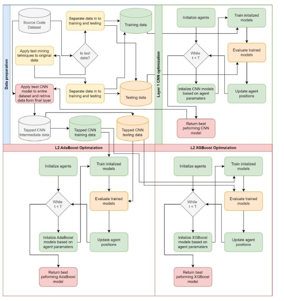
3.3. Proposed Experimental Optimization Framework
The framework proposed in this work utilized a two layer approach. The first layer focuses on CNN optimization. Metaheuristics optimizes are applied to parameter selection of CNN. Data is processed and prepared accordingly. Text data is suitably encoded and CNN optimization is carried out in the first layer of the framework.
Once a suitable CNN model is generated, it is applied to the whole dataset and the final layer tapped to recover intermediate data. This intermediate data is then used as inputs for XGBoost and AdaBoost optimizes. Separate optimizations are carried for each classifier. Further details of the experimental setup are provided in the following section. A flowchart of the porpoised framework is provided in Figure 2.
4. Experimental Setup
In this work two separate simulations are carried out. The first set of simulations is conducted using the a group of 5 datasets which are KC1, JM1, CM1, KC2, and PC1. These datasets are part of NASA’s promise repository aimed at SDP. The instances in datasets represent various software models and the features depict the quality of that code. McCabe [36] and Halstead [37] metrics were applied through 22 features. The McCabe approach was applied to its methodology that emphasizes less complex code through the reduction of pathways, while Halstead uses counting techniques as the logic behind it was that the larger the code the more it is error-prone. A tow layer approach is applied to these simulations. The class balance in the utilized dataset is provided in Figure 3. The first utilized dataset is dis balanced with 22.5% of samples representing software with errors and 77.5% without.
A correlational heat map of the features is provided in Figure 4.
The second set of simulation utilized a dataset comprised of around 1000 crowd-sourced Python programming problems. The dataset is publicly available 1, and last accessed on the 01.08.2024. The problems are on the beginner level and consist of a description of the task, the solution, and 3 automated test cases. A generative model based on GPT-2 is used to generate solutions to these problems based off descriptive problems. Generated solutions that pass as well as fail at least one test case are collected and combined in to a unified dataset. The resulting dataset combines ground truth solutions with generated code that has some errors. The final combined dataset is comprised of 10000 samples and is balanced.
Both datasets are separated in to training and testing portions for simulations. An initial 70% of data is used for training and a later 30% for evaluation. Evaluations are carried out using a standard set of classification evaluation metrics including accuracy, recall, f1-score and precision. The Matthews correlation coefficient (MCC) metric is used as the objective function that can be determined as per 22. An indicator function is also tracked. The indicator function is the Cohen’s kappa which is determined as per Eq. 23. Metaheuristics are tasked with selecting optimal parameters, maximizing the MCC score.
here true positives (TP) denotes samples correctly classified as positive, true negatives (TN) denotes instances correctly classified as negative. Similarly false positives (FP) and false negatives (FN) denote samples incorrectly classified as positive and negative respectively.
In the first layer CNN parameters are optimized. The respective parameters and their constraints are provided in Table 1.
In the second optimization layer, intermediate outputs of the CNN are used. The final dense layer is recorded during classifications of all the samples available in the dataset. This is once again separated in to 70% for training and 30% for testing. These are then utilized to training and optimize AdaBoost and XGBoost models. Parameter ranges for AdaBoost and XGBoost are provided in Table 2 and Table 3 respectively.
Several optimizers are included in a comparative analysis against the proposed modified algorithm. These include the original PSO [32], as well as several other established optimizers such as the GA [34] and VNS [15]. Additional optimizers included in the comparison are the ABC [16], BA [17] and COLSHADE [18] optimizers. A recently proposed SCHO [19] optimizer is also explored. Each optimizer is implemented using original parameter settings suggested in the works that introduced said algorithm. Optimizes are allocated a population size of 10 agents and allowed a total of 8 iterations to locate promising outcomes within the given search range. Simulations are carried out through 30 independent executions to facilitate further analysis.
For NLP simulations, only a the second layer of the framework is utilized. Input text is encoded using TF-IDF encoding to a maximum of 1000 tokens. These are used as inputs for model training and evaluation. Optimization is carried out using the second layer of the introduced framework and a comparative analyses is conducted under identical conditions as previous simulations to demonstrate the flexibility of the proposed approach.
5. Simulation Outcomes
The following subsections present the simulation outcomes of the conducted simulation. First outcomes of the simulations with traditional dataset are conducted in a two layer approach. Secondly two simulations with NLP are presented using only the second layer of the framework.
5.1. Layer One CNN Simulations
First layer CNN optimization outcomes in terms of objective function are provided in Table 4. The introduced MPPSO demonstrates most favorable outcomes, attaining an objective metric score of 0.273280 in the best case execution, and 0.262061 in the worst. In turn score in the mean and median are also the best with 0.268824 and 0.269873 respectively. The highest stability rate is demonstrated by the SCHO optimizer, however, this optimizer does not manage to match the favorable outcomes demonstrated by other algorithms, suggesting a lack of exploration of exploitation potential.
First layer CNN optimization outcomes in terms of indicator function are provided in Table 5. The introduced MPPSO demonstrates similarly favorable results attaining the best outcomes with a score of 0.231201. Mean and median scores of 0.233446 and 0.232697 are also the best among evaluated optimizes. A high rate of stability in terms of indicator metric is demonstrated by the original PSO, however the performance of the modified version descend that of the original in all cases.
Visual comparisons in terms of optimizer stability is provided in Figure 5. While the stability of the introduced optimizer is not the highest compared to all other optimizes, algorithms with higher rates of stability attain less favorable outcomes. This suggests that VNS, BA, and COLSHADE for instance overly focus on local optima rather then looking for more favorable outcomes. This lack of exploration leads to higher stability but less favorable outcomes in this test case. The introduced optimizer also outperformed the base PSO while demonstrating higher stability, suggesting that the introduced modification has a positive influence on performance.
Convergence rate of algorithms provide valuable feedback on optimizer behaviour. Convergence rates for both the objective and indicator functions are tracked and provided in Figure 6 and Figure 7 for each optimizer. The introduced optimizer demonstrates favorable performance locating the best solution by iteration eight. Other optimizes stagnate prior to reaching favorable outcomes, suggesting that the boost in exploration incorporated in to the MPPSO helps overcome the shortcomings inherent to the original PSO. Similar conclusions can be made in terms of indicator function convergence demonstrated in Figure 7. As the indicator function was not the target of the optimization, there is a small decrease in the first iteration of the optimization. However, the best best outcome of the the comparison is once again located by the introduced optimizer by iteration 3.
Comparisons between the best preforming models optimized by each algorithm included in the comparative analysis is provided in Table 6. The introduced optimize demonstrates a clear dominance in terms of accuracy as well as precision. However, other optimizers demonstrate certain favorable characterises as well, which is to be somewhat expected and further supports the NFL theorem of optimization.
Further details for the best performing model optimized by the MPPSO algorithm are provided in the form of the ROC curve and confusion matrix provided in Figure 8 and Figure 9. A plot of the best performing model is also provided in Figure 10. Finally, to support simulation repeatability, the parameter selections made by each optimizer for their respective best performing optimized models is provided in Table 7.
5.2. Layer Two Simulations
Once a suitable CNN model is trained, the final layer is utilized as inputs for AdaBoost and XGBoost classifiers. These classifiers are themselves subjected to hyperparameter optimization using a set of metaheursitic optimizers. This process in done in the second layer of the optimization framework. The following subsections present the outcomes of these simulations.
5.2.1. AdaBoost Layer 2 Classifications
The outcomes of AdaBoost model optimization in terms of objective function are provided in Table 8. The introduced MPPSO demonstrates the best outcomes in the worst, mean and median scenarios, attaining scores of 0.276185, 0.279771 and 0.280600 respectively. In terms of the best performing model, the MPPSO and original PSO managed to attain models that match performance. The highest stability rate is demonstrated by the SCHO, however, this optimizer does not manage to match the favorable outcomes demonstrated by other algorithms, suggesting a lack of exploration of exploitation potential.
Second layer AdaBoost optimization outcomes in terms of indicator function are provided in Table 9. Interestingly, in terms of indicator function outcomes the BA demonstrates Superior performance to all tested algorithms. However, since this was not the goal and metric of the optimisation process these findings are quite interesting and further support the NFL theorem. High stability rates are demonstrated by the SCHO algorithm.
Visual comparisons in terms of optimizer stability are provided in Figure 11. Two interesting spikes in objective function distributions can be observed in the introduced optimizer outcomes. Interestingly, other optimizer overly focus on the first (lower) region. However, the introduced optimizer overcomes these limitations and locates a more promising region. The BA locates a promising region within the aerospace. However, the BA stability greatly sufferers providing by far the lowest stability compared to other evaluated optimizers leading to overall mixed results.
Convergence rates for both the objective and indicator functions for L2 adaboost optimizations are tracked and provided in Figure 12 and Figure 13 for each optimizer. The porpoised MPPSO shows a favorable rate of convergence, locating a good solution by iterations 7, and further improving on this solution in iteration 19. While other optimizers manage to find decent outcomes, a fast rate of convergence limits the quality of the located solution. Similar conclusions can be made in terms of indicator function convergence demonstrated in Figure 13 where the optimizer once again locates the pest solution near the end of the optimization in iteration 19.
Comparisons between the best preforming AdaBoost L2 models optimized by each algorithm included in the comparative analysis is provided in Table 10. The best performing models match performance across several metrics suggesting that several optimizers are equally well suited for AdaBoost optimization demonstrating a favorable accuracy of 0.772166 outperforming scored attained by using just CNN in L1.
Further details for the best performing adaboost L2 model optimized by the MPPSO algorithm are provided in the form of the ROC curve and confusion matrix provided in Figure 14 and Figure 15. Finally, to support simulation repeatability, the parameter selections made by each optimizer for their respective best performing optimized models is provided in Table 11.
5.2.2. XGBoost Layer 2 Classifications
The outcomes of XGBoost L2 model optimization in terms of objective function are provided in Table 13. The introduced MPPSO demonstrates the best outcomes in the best case simulation with an objective function score of 0.283956. Interestingly in terms of worst, mean and median fictions the VNS algorithm demonstrates the most favorable outcomes. In turn this algorithm also demonstrates a high rate of stability in the conducted simulations on this challenge.
Second layer XGBoost optimization outcomes in terms of indicator function are provided in Table 13. The introduced optimizer does not attain the best outcomes in terms of indicator function results, as the ABC algorithm attains the most favorable results. These interesting findings further support the NFL theorem indicating that no single approach is equally suited to all challenges and across all metrics. In terms of indicator function stability, the PSO attained the best outcomes.
Visual comparisons in terms of optimizer stability is provided in Figure 16. While the introduced optimizer attains more favorable outcomes in terms of objective function, an evident disadvantage can be observed in comparison to the original PSO, with the PSO algorithm favoring a better location within the search space in more cases. An overall low stability can be observed for the BA algorithm, while the ABC algorithm focuses of a sub optimal search space in many solution instances.
Convergence rates for both the objective and indicator functions for L2 XGBoost optimizations are tracked and provided in Figure 17 and Figure 18 for each optimizer. The introduced optimize manages to find a promising region in the 19 iteration, surpassing solutions located by other algorithms. However, this improvement comes at a cost of indicator function outcomes, where the performance is slightly reduced. Often times the trade off in terms of one metric can mean improvements in another. As the indicator function was not the primary goal of the optimisation the MPPSO algorithm attained favorable optimization performance overall.
Comparisons between the best preforming XGBoost L2 models optimized by each algorithm included in the comparative analysis is provided in Table 14. The favorable performance of the VNS algorithm is undeniable for this challenge further supporting the NFL theorem of optimization. Nevertheless, constant experimentation is needed to determined suitable optimizers for any given problem. Furthermore, it is important to consider all the metrics when determining which algorithm is the best suited to the demands of a given optimization challenge.
Further details for the best performing XGBoost L2 model optimized by the MPPSO algorithm are provided in the form of the ROC curve and confusion matrix provided in Figure 19 and Figure 20. Finally, to support simulation repeatability, the parameter selections made by each optimizer for their respective best performing optimized models is provided in Table 23.
5.3. Simulations with NLP
The second layer of the framework is also utilized in conjunction with text mining techniques to handle NLP. Encoding is handled using TF-IDF vectorization to a limit of 1000 features. Vectorized values are then used as inputs to the second layer of the framework where AdaBoost and XGBoost are used to handled classifications. Optimization is carried out on these classification models to improve overall performance though parameter selection.
5.3.1. AdaBoost NLP Classifications
The outcomes of AdaBoost NLP classifier model optimization in terms of objective function are provided in Table 16. The introduced MPPSO demonstrates the best outcomes in the best case simulation with an objective function score of 0.959947 alongside the BA optimizer. In terms of stability as well as the works, and mean outcomes the original PSO demonstrates favorable performance, while the BA attain the best results for the median performance. The PSO also demonstrates a high rate of stability in terms of objective scores.
AdaBoost NLP classifier optimization outcomes in terms of indicator function are provided in Table 17. High stability rates are showcased by the PSO and favorable outcomes by the VNS algorithm, attaining the best overall indicator score, as well as the ABC that demonstrates the best outcomes in the worst case execution.
Visual comparisons in terms of AdaBoost NLP optimizer stability is provided in Figure 21. High stability rates are demonstrated by the PSO, however, the best scores are still located by the modified optimizer suggesting that modification hold further potential. A trade off is always present when tackling multiple optimizations problems it is essential to explore multiple potential optimizes in order to determine a suitable approach, as stated by the NFL theorem.
Convergence rates for both the objective and indicator functions for NLP AdaBoost optimizations are tracked and provided in Figure 22 and Figure 23 for each optimizer. While all optimizes show a favorable convergence rate several optimizers dwell in sub optimal regions within the search space. The introduced optimizer overcomes the local minimum issue and locates a promising solution in the 18 iteration of the optimisation. Similar operations can be made in terms of indicator functions with the best solution located by the optimizer in the latter iterations.
Comparisons between the best preforming AdaBoost NLP classifier models optimized by each algorithm included in the comparative analysis is provided in Table 18. Favorable outcomes can be observed for all evaluated models suggesting that metaheuristic optimizers, as well as the AdaBoost classifier are well suited to problem of error detection through applied NLP.
Further details for the best performing AdaBoost NLP classifier model optimized by the MPPSO algorithm are provided in the form of the ROC curve and confusion matrix provided in Figure 24 and Figure 25. Finally, to support simulation repeatability, the parameter selections made by each optimizer for their respective best performing optimized models is provided in Table 23.
5.3.2. XGBoost NLP Classifications
The outcomes of XGBoost NLP classifier model optimization in terms of objective function are provided in Table 20. The introduced optimizer demonstrates the most favorable outcomes for the best case scenario. Nevertheless, the original PSO demonstrates overall favorable scores across all other test scenarios. Accordingly, the overall stability of the PSO is also equally favorable, with the highest rates of stability in compassion to other optimizes.
XGBoost NLP classifier optimization outcomes in terms of indicator function are provided in Table 21. High stability rates are demonstrated by the PSO, while the ABC algorithm demonstrates the best scores across all other metrics for the indicator function.
Visual comparisons in terms ofXGBoost NLP optimizer stability is provided in Figure 26. While the best scores in the best case scenario are showcased by the introduced optimizer, PSO outcomes are also favorable, with many solutions overcoming local optima and locating more promising outcomes overall.
Convergence rates for both the objective and indicator functions for NLP XGBoost optimizations are tracked and provided in Figure 27 and Figure 28 for each optimizer. The introduced optimizer overcomes local minimum traps, locating a favorable outcomes in iteration 18, suggesting that the boost in exploration especially in later stages helps overall performance improve, while the baseline PSO sticks to a less favorable regions. These outcomes are mirrored in terms of indicator function with the best solution determined by the introduced optimiser in the 18 iteration.
Comparisons between the best preforming XGBoost NLP classifier models optimized by each algorithm included in the comparative analysis is provided in Table 22. The best performance is demonstrated by the introduced optimizer across many metrics attaining an accuracy of 0.983893. The GA also demonstrated good performance in terms of precision for non error and recall for errors in code further affirming the NFL theorem.
Further details for the best performing XGBoost NLP classifier model optimized by the MPPSO algorithm are provided in the form of the ROC curve and confusion matrix provided in Figure 29 and Figure 30. Finally, to support simulation repeatability, the parameter selections made by each optimizer for their respective best performing optimized models is provided in Table 15.
5.4. Statistical Validation
When comparison algorithms that rely on randomness, such as metaheuristics, it is essential to verify the statistical significance of findings as a single simulation may not be representative of overall performance. With this in mind, simulations in this work are carried out in 30 individually independent runs and data collected for further analysis.
Two types of statistical test can be applied to validate statistical significance of outcomes, parametric and non-parametric test. The first step, therefore, involves validating that the safe used of parametric tests is warranted or if non-parametric analysis should be applied. The used of parametric tests is justified if conditions of independence, normality, and homoscedasticity [38] are met. As all simulations are conducted using independent random seeds the independence criteria is met. Homoscedasticity is confirmed via Levene’s test [39] which resulted in a of 0.68 for each case, indicating that this condition is also met.
The last conduction, normality, is assessed using the Shapiro-Wilk’s test [40], with computed for each method included in the comparative analysis. As all the values are bellow a threshold of the null hypothesis (H0) may be rejected, suggesting outcomes do not originate form normal distributions. These findings are further enforced by the objective function KDE diagrams presented in Figure 31. The outcomes of the Shapiro-Wilk test are provided in Table 24.
As one of the criteria needed to justify the safe use of parametric tests is not met further evaluations are conducted via non-parametric tests. The Wilcoxon signed-rank test is therefore applied to compare the performance of the MPPSO to other algorithms included in the comparative analysis. Test scores are presented in Table 25. A threshold of is not exceeded in any of the test cases indicating that the outcomes attained by the MPPSO algorithm hold statistically significant improvements over other evaluated methods.
5.5. Best Model Interpretations
Model interpretation plays an increasingly important role in modern IA research. Often times understanding the factors and their degree of influence on decision can help better understand the problem at hand, as well as detect any unintended biases in data. There are several emerging techniques for interpreting models, and for simpler models these interpretations are fairly straight-forward. However, more complicated models, and models that utilize a multi-tier framework can be more difficult to subject to interpretation.
This work utilizes SHAP analysis in order to determined feature importance and feature impact on optimized model decisions. SHAP analysis utilizes an approach rooted in game theory treating features as contestants in a cooperative competition. The contributions of each features as well as their collaborative contributions are considered when determining importance. Importance can also be analyzed on a global and local level making SHAP a versatile and promising approach for model analysis.
Feature importances for the best performing models constructed in L1 and L2 simulations are provided in Figure 32. Each constructed classifier places a slightly different importance of each feature. However, I, Uniq_OP, IOBland and d are universally highly ranked. The best CNN adn AdaModels show the highest impact for the I feature while this feature is second best for the XGBoost classifier, with the highest importance placed on uniq_OP feature.
Feature importances for the best performing models in NLP simulations are likewise provided in Figure 33 for the AdaBoost model and in Figure 34 for the XGBoost model. TF-IDF vectorized feature importances are once again interpreted using SHAP analysis and the top 20 contributing features shown for both models. Both models place a high importance on the def keyword, as well as the print and write keywords where errors can often occur. The AdaBoost model places a significant importance of the def keyboard, with print holding the second spot with a significantly lower importance. The XGBoost model however has a more even distribution of importance. While def holds a high importance the second highest impact is on the write keyword followed by print with a slightly decreased importance.
Understanding feature importance on model decisions can further aid in understanding the challenges associated with software defect detection. Furthermore, determining what features play and important role in these classifications can further aid in reducing computational costs of models in deployment as well as aid in improving data collection in the future. Detecting hidden model biases is also essential for enforcing trust in model decisions improving the generalizability and objectivity of decisions.
6. Conclusion
Software has become increasingly integral to societal infrastructure, governing critical systems. Ensuring the reliability of software is therefore paramount across various industries. As the demand for accelerated development intensifies, the manual review of code presents growing challenges, with testing frequently consuming more time than development. A promising method for detecting defects at the source code level involves the integration of AI with NLP. Given that software is composed of human-readable code, which directs machine operations, the validation of the highly diverse machine code on a case-by-case basis is inherently complex. Consequently, source code analysis offers a potentially effective approach to improving defect detection and preventing errors.
This work explores the advantages and challenges of utilizing AI for error detection in software code. Both classical and NLP methods are explored on two publicly available dataset with 5 experiments total conducted. A two layer optimization framework is introduced in order to manage the complex demands of error detection. A CNN architecture is utilized in the first layer to help process the large amounts of data in a more computational efficient manner, with the second layer handling intermediate results using AdaBoost and XGBoost classifiers. An additional set of simulations using only the second layer of the framework in combination with TF-IDF encoding is also carried out in order to provide a comparison between emerging NLP and classical techniques. As optimizer performance is highly dependant on adequate parameter selection, a modified version of the well established PSO is introduced, designed specifically for the needs of this research and with an aim to overcome some of the known drawback of the original algorithm. A comparative analysis is carried out with several state of the art optimizes with the introduced approach demonstrative promising outcomes in several simulations.
Twin layer simulations improve upon the baseline outcomes demonstrated by CNN boost accuracy form 0.768799 to 0.772166 for the AdaBoost models and 0.771044 for the XGBoost best performing classifier. This suggests that a two layer approach can yield favorable outcomes while maintaining favorable computational demands in comparison to more complex network solutions. Optimization carried out using NLP demonstrate an impressive accuracy of 0.979781 for the best performing AdaBoost model and a 0.983893 for the best performing XGBoost model. Simulations are further validated using statistical evaluation to confirm the significance of the observations. The best preforming models are also subjected to SHAP analysis to determine feature importance and help locate any potential hidden biases within the best performing models.
It is worth noting that the extensive computational demands of the optimizations carried out in this work limit the extend of optimizers that can be tested. Further limitations are associated with population sized and allocated numbers of iterations for each optimization due to hardware memory limitations. Future works hope to address these concerns as additional resources become available. Additional implementations of the proposed MPPSO hope to be explored for other implementations. Emerging transformer based architectures based on custom BERT encoding also hope to be explored for software defect detection in future works.
References
- Alyahyan, S.; Alatawi, M.N.; Alnfiai, M.M.; Alotaibi, S.D.; Alshammari, A.; Alzaid, Z.; Alwageed, H.S. Software reliability assessment: An architectural and component impact analysis. Tsinghua Science and Technology 2024. [Google Scholar] [CrossRef]
- Zhang, H.; Gao, X.Z.; Wang, Z.; Wang, G. Guest Editorial of the Special Section on Neural Computing-Driven Artificial Intelligence for Consumer Electronics. IEEE Transactions on Consumer Electronics 2024, 70, 3517–3520. [Google Scholar] [CrossRef]
- Mcmurray, S.; Sodhro, A.H. A study on ML-based software defect detection for security traceability in smart healthcare applications. Sensors 2023, 23, 3470. [Google Scholar] [CrossRef]
- Giray, G.; Bennin, K.E.; Köksal, Ö.; Babur, Ö.; Tekinerdogan, B. On the use of deep learning in software defect prediction. Journal of Systems and Software 2023, 195, 111537. [Google Scholar] [CrossRef]
- Jim, J.R.; Talukder, M.A.R.; Malakar, P.; Kabir, M.M.; Nur, K.; Mridha, M. Recent advancements and challenges of nlp-based sentiment analysis: A state-of-the-art review. Natural Language Processing Journal, 2024; 100059. [Google Scholar]
- Wolpert, D.H.; Macready, W.G. No free lunch theorems for optimization. IEEE transactions on evolutionary computation 1997, 1, 67–82. [Google Scholar] [CrossRef]
- Zivkovic, T.; Nikolic, B.; Simic, V.; Pamucar, D.; Bacanin, N. Software defects prediction by metaheuristics tuned extreme gradient boosting and analysis based on Shapley Additive Explanations. Applied Soft Computing 2023, 146, 110659. [Google Scholar] [CrossRef]
- Ali, M.; Mazhar, T.; Al-Rasheed, A.; Shahzad, T.; Ghadi, Y.Y.; Khan, M.A. Enhancing software defect prediction: a framework with improved feature selection and ensemble machine learning. PeerJ Computer Science 2024, 10, e1860. [Google Scholar] [CrossRef]
- Khleel, N.A.A.; Nehéz, K. Software defect prediction using a bidirectional LSTM network combined with oversampling techniques. Cluster Computing 2024, 27, 3615–3638. [Google Scholar] [CrossRef]
- Zhang, Q.; Zhang, J.; Feng, T.; Xue, J.; Zhu, X.; Zhu, N.; Li, Z. Software Defect Prediction Using Deep Q-Learning Network-Based Feature Extraction. IET Software 2024, 2024, 3946655. [Google Scholar] [CrossRef]
- Briciu, A.; Czibula, G.; Lupea, M. A study on the relevance of semantic features extracted using BERT-based language models for enhancing the performance of software defect classifiers. Procedia Computer Science 2023, 225, 1601–1610. [Google Scholar] [CrossRef]
- Dash, G.; Sharma, C.; Sharma, S. Sustainable marketing and the role of social media: an experimental study using natural language processing (NLP). Sustainability 2023, 15, 5443. [Google Scholar] [CrossRef]
- Velasco, L.; Guerrero, H.; Hospitaler, A. A literature review and critical analysis of metaheuristics recently developed. Archives of Computational Methods in Engineering 2024, 31, 125–146. [Google Scholar] [CrossRef]
- Jain, V.; Kashyap, K.L. Ensemble hybrid model for Hindi COVID-19 text classification with metaheuristic optimization algorithm. Multimedia Tools and Applications 2023, 82, 16839–16859. [Google Scholar] [CrossRef]
- Mladenović, N.; Hansen, P. Variable neighborhood search. Computers & operations research 1997, 24, 1097–1100. [Google Scholar]
- Karaboga, D.; Akay, B. A comparative study of artificial bee colony algorithm. Applied mathematics and computation 2009, 214, 108–132. [Google Scholar] [CrossRef]
- Yang, X.S.; Hossein Gandomi, A. Bat algorithm: a novel approach for global engineering optimization. Engineering computations 2012, 29, 464–483. [Google Scholar] [CrossRef]
- Gurrola-Ramos, J.; Hernàndez-Aguirre, A.; Dalmau-Cedeño, O. COLSHADE for real-world single-objective constrained optimization problems. In Proceedings of the 2020 IEEE congress on evolutionary computation (CEC). IEEE; 2020; pp. 1–8. [Google Scholar]
- Bai, J.; Li, Y.; Zheng, M.; Khatir, S.; Benaissa, B.; Abualigah, L.; Wahab, M.A. A sinh cosh optimizer. Knowledge-Based Systems 2023, 282, 111081. [Google Scholar] [CrossRef]
- Damaševičius, R.; Jovanovic, L.; Petrovic, A.; Zivkovic, M.; Bacanin, N.; Jovanovic, D.; Antonijevic, M. Decomposition aided attention-based recurrent neural networks for multistep ahead time-series forecasting of renewable power generation. PeerJ Computer Science 2024, 10. [Google Scholar] [CrossRef]
- Gajevic, M.; Milutinovic, N.; Krstovic, J.; Jovanovic, L.; Marjanovic, M.; Stoean, C. Artificial neural network tuning by improved sine cosine algorithm for healthcare 4.0. In Proceedings of the Proceedings of the 1st international conference on innovation in information technology and business (ICIITB 2022). Springer Nature, 2023, Vol.104; p. 2023104289.
- Minic, A.; Jovanovic, L.; Bacanin, N.; Stoean, C.; Zivkovic, M.; Spalevic, P.; Petrovic, A.; Dobrojevic, M.; Stoean, R. Applying recurrent neural networks for anomaly detection in electrocardiogram sensor data. Sensors 2023, 23, 9878. [Google Scholar] [CrossRef]
- Jovanovic, L.; Milutinovic, N.; Gajevic, M.; Krstovic, J.; Rashid, T.A.; Petrovic, A. Sine cosine algorithm for simple recurrent neural network tuning for stock market prediction. In Proceedings of the 2022 30th Telecommunications Forum (TELFOR). IEEE; 2022; pp. 1–4. [Google Scholar]
- Jovanovic, L.; Djuric, M.; Zivkovic, M.; Jovanovic, D.; Strumberger, I.; Antonijevic, M.; Budimirovic, N.; Bacanin, N. Tuning xgboost by planet optimization algorithm: An application for diabetes classification. In Proceedings of the Proceedings of fourth international conference on communication, computing and electronics systems: ICCCES 2022. Springer; pp. 2023787–803.
- Pavlov-Kagadejev, M.; Jovanovic, L.; Bacanin, N.; Deveci, M.; Zivkovic, M.; Tuba, M.; Strumberger, I.; Pedrycz, W. Optimizing long-short-term memory models via metaheuristics for decomposition aided wind energy generation forecasting. Artificial Intelligence Review 2024, 57, 45. [Google Scholar] [CrossRef]
- Devlin, J.; Chang, M.W.; Lee, K.; Toutanova, K. Bert: Pre-training of deep bidirectional transformers for language understanding. arXiv preprint arXiv:1810.04805, arXiv:1810.04805 2018.
- Aftan, S.; Shah, H. A survey on bert and its applications. In Proceedings of the 2023 20th Learning and Technology Conference (L&T). IEEE, 2023; pp. 161–166.
- Mittal, S.; Stoean, C.; Kajdacsy-Balla, A.; Bhargava, R. Digital assessment of stained breast tissue images for comprehensive tumor and microenvironment analysis. Frontiers in bioengineering and biotechnology 2019, 7, 246. [Google Scholar] [CrossRef] [PubMed]
- Postavaru, S.; Stoean, R.; Stoean, C.; Caparros, G.J. Adaptation of deep convolutional neural networks for cancer grading from histopathological images. In Proceedings of the Advances in Computational Intelligence: 14th International Work-Conference on Artificial Neural Networks, IWANN 2017, Cadiz, Spain, June 14-16 2017, Proceedings, Part II 14. Springer, 2017; pp. 38–49.
- Freund, Y.; Schapire, R.E. A desicion-theoretic generalization of on-line learning and an application to boosting. In Proceedings of the European conference on computational learning theory. Springer; 1995; pp. 23–37. [Google Scholar]
- Chen, T.; Guestrin, C. Xgboost: A scalable tree boosting system. In Proceedings of the Proceedings of the 22nd acm sigkdd international conference on knowledge discovery and data mining, 2016, pp.; pp. 785–794.
- Kennedy, J.; Eberhart, R. Particle swarm optimization. In Proceedings of the Proceedings of ICNN’95-international conference on neural networks. ieee, 1995, Vol.4; pp. 1942–1948.
- Bacanin, N.; Simic, V.; Zivkovic, M.; Alrasheedi, M.; Petrovic, A. Cloud computing load prediction by decomposition reinforced attention long short-term memory network optimized by modified particle swarm optimization algorithm. Annals of Operations Research, 2023; 1–34. [Google Scholar]
- Mirjalili, S.; Mirjalili, S. Genetic algorithm. Evolutionary algorithms and neural networks: theory and applications, 2019; 43–55. [Google Scholar]
- Rahnamayan, S.; Tizhoosh, H.R.; Salama, M.M.A. Quasi-oppositional Differential Evolution. In Proceedings of the 2007 IEEE Congress on Evolutionary Computation; 2007; pp. 2229–2236. [Google Scholar] [CrossRef]
- McCabe, T. A Complexity Measure. IEEE Transactions on Software Engineering 1976, 2, 308–320. [Google Scholar] [CrossRef]
- Halstead, M. Elements of Software Science; Elsevier, 1977.
- LaTorre, A.; Molina, D.; Osaba, E.; Poyatos, J.; Del Ser, J.; Herrera, F. A prescription of methodological guidelines for comparing bio-inspired optimization algorithms. Swarm and Evolutionary Computation 2021, 67, 100973. [Google Scholar] [CrossRef]
- Glass, G.V. Testing homogeneity of variances. American Educational Research Journal 1966, 3, 187–190. [Google Scholar] [CrossRef]
- Shapiro, S.S.; Francia, R. An approximate analysis of variance test for normality. Journal of the American statistical Association 1972, 67, 215–216. [Google Scholar] [CrossRef]
Figure 1.
Crossover and mutation mechanisms.
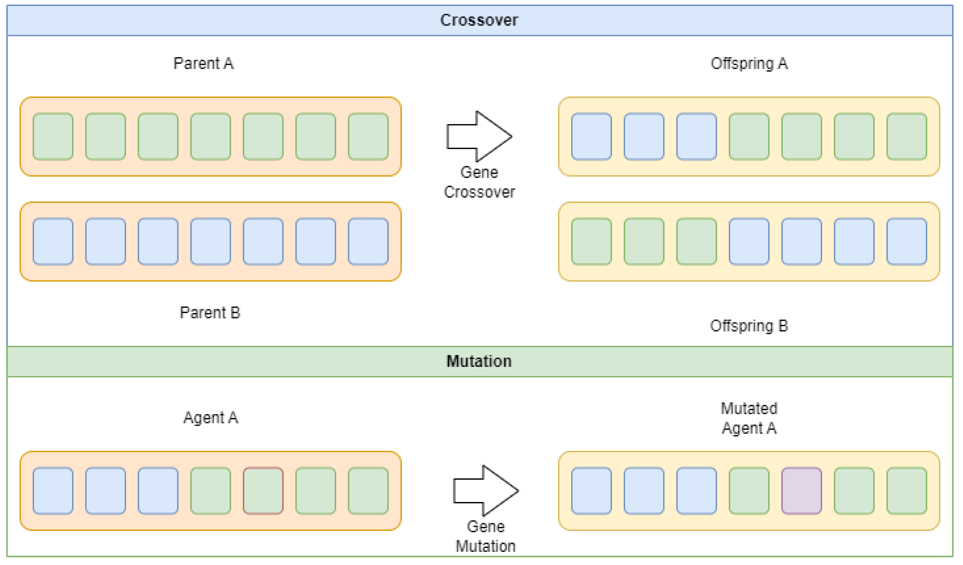
Figure 2.
Proposed optimization framework flowchart
Figure 3.
Class distribution in NASA dataset.
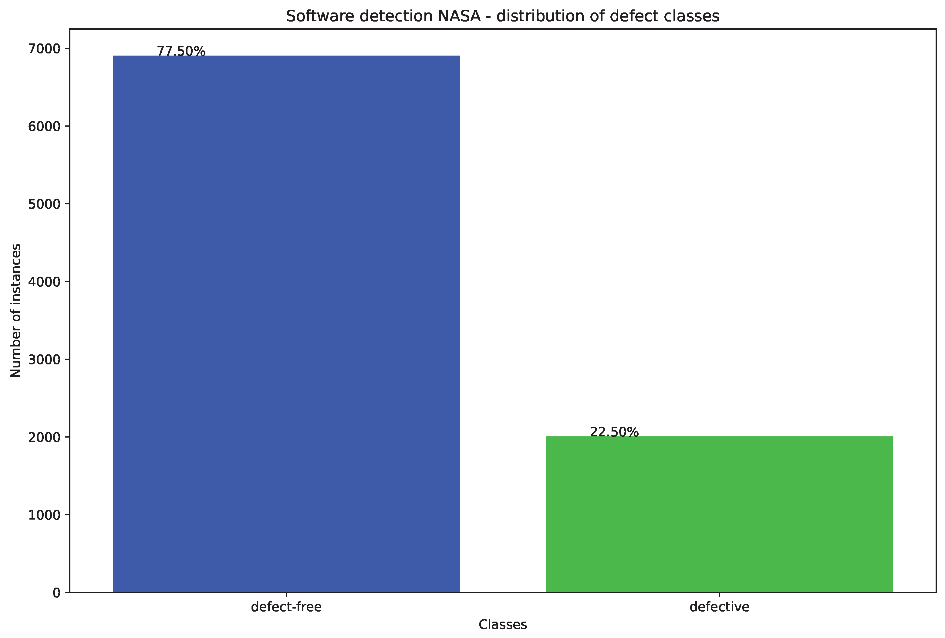
Figure 4.
NASA feature correlation heat-map.
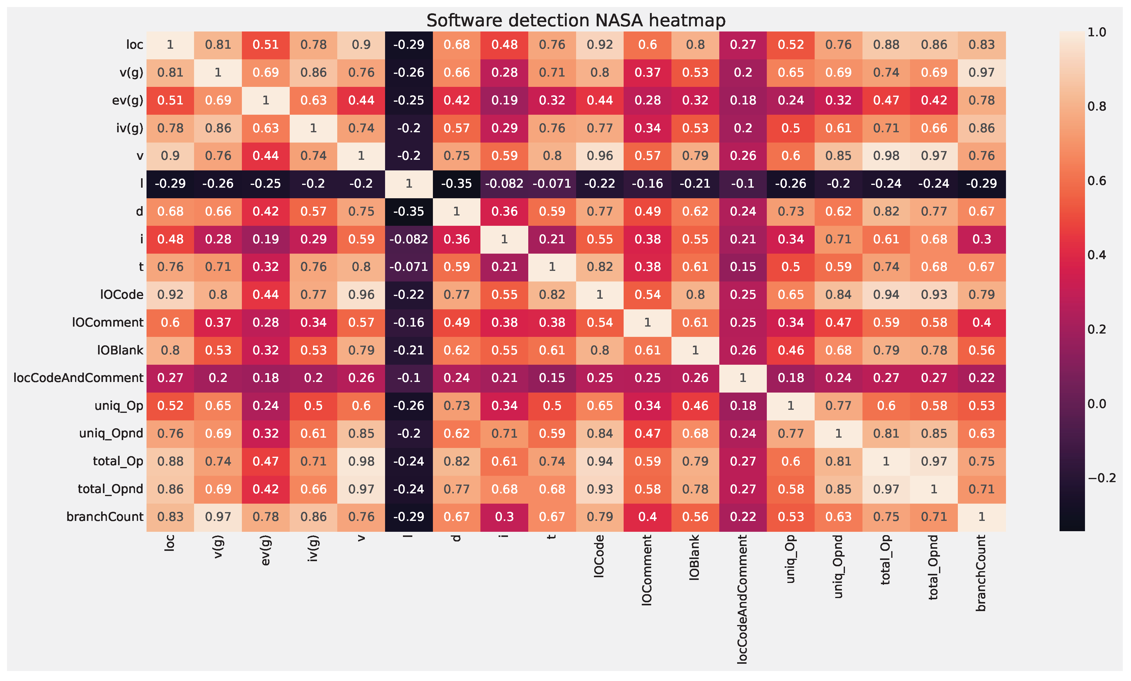
Figure 5.
Layer 1 (CNN) objective and indicator outcome distributions.
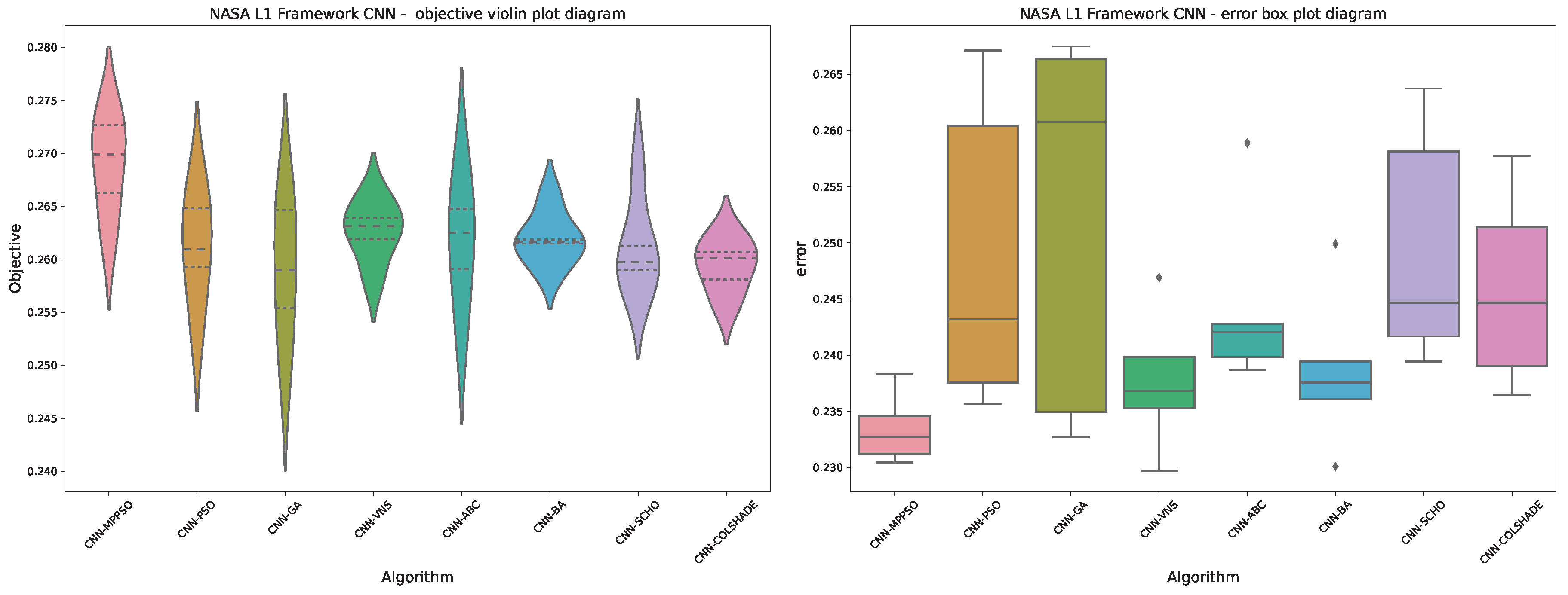
Figure 6.
Layer 1 (CNN) objective function convergence.
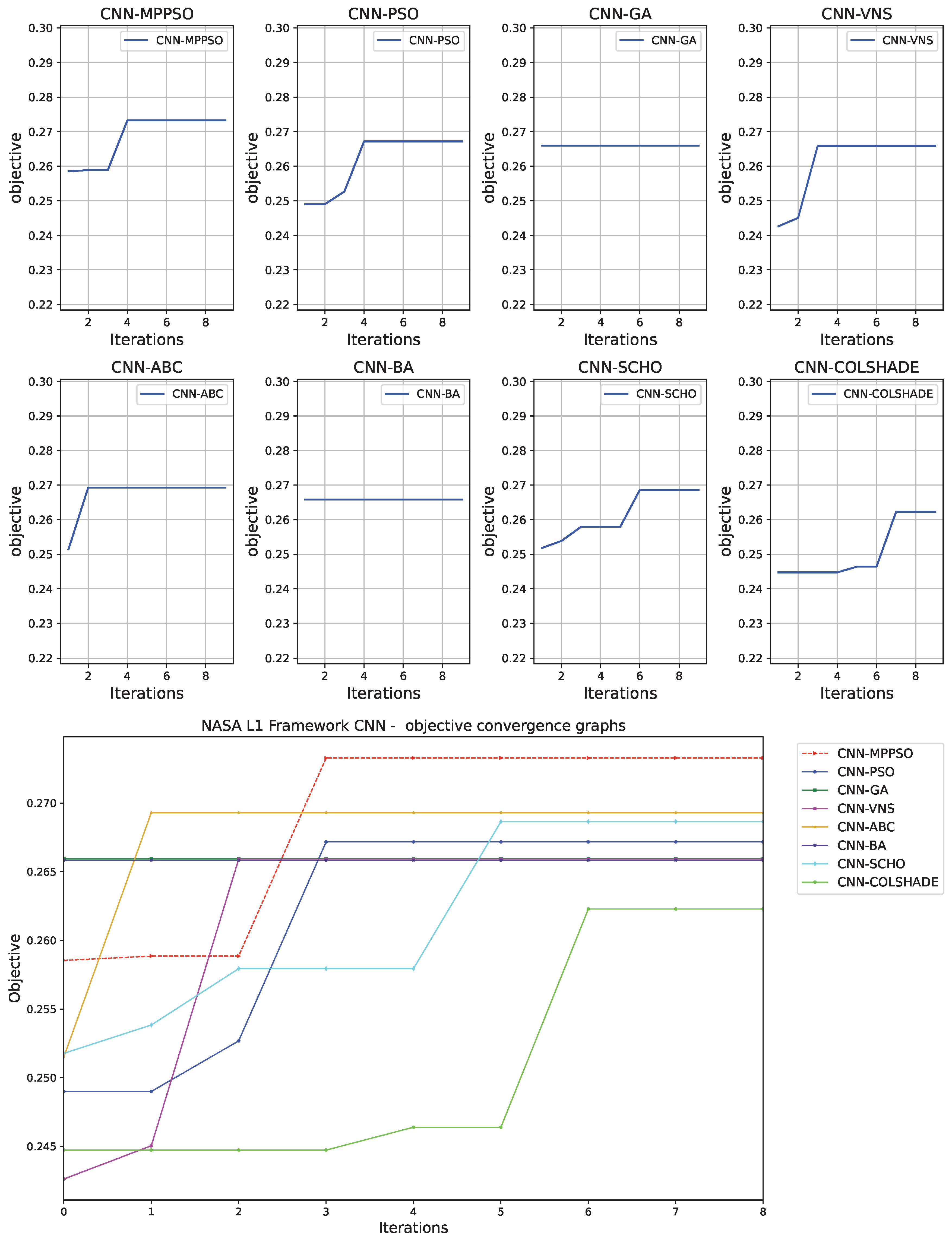
Figure 7.
Layer 1 (CNN) indicator function convergence.
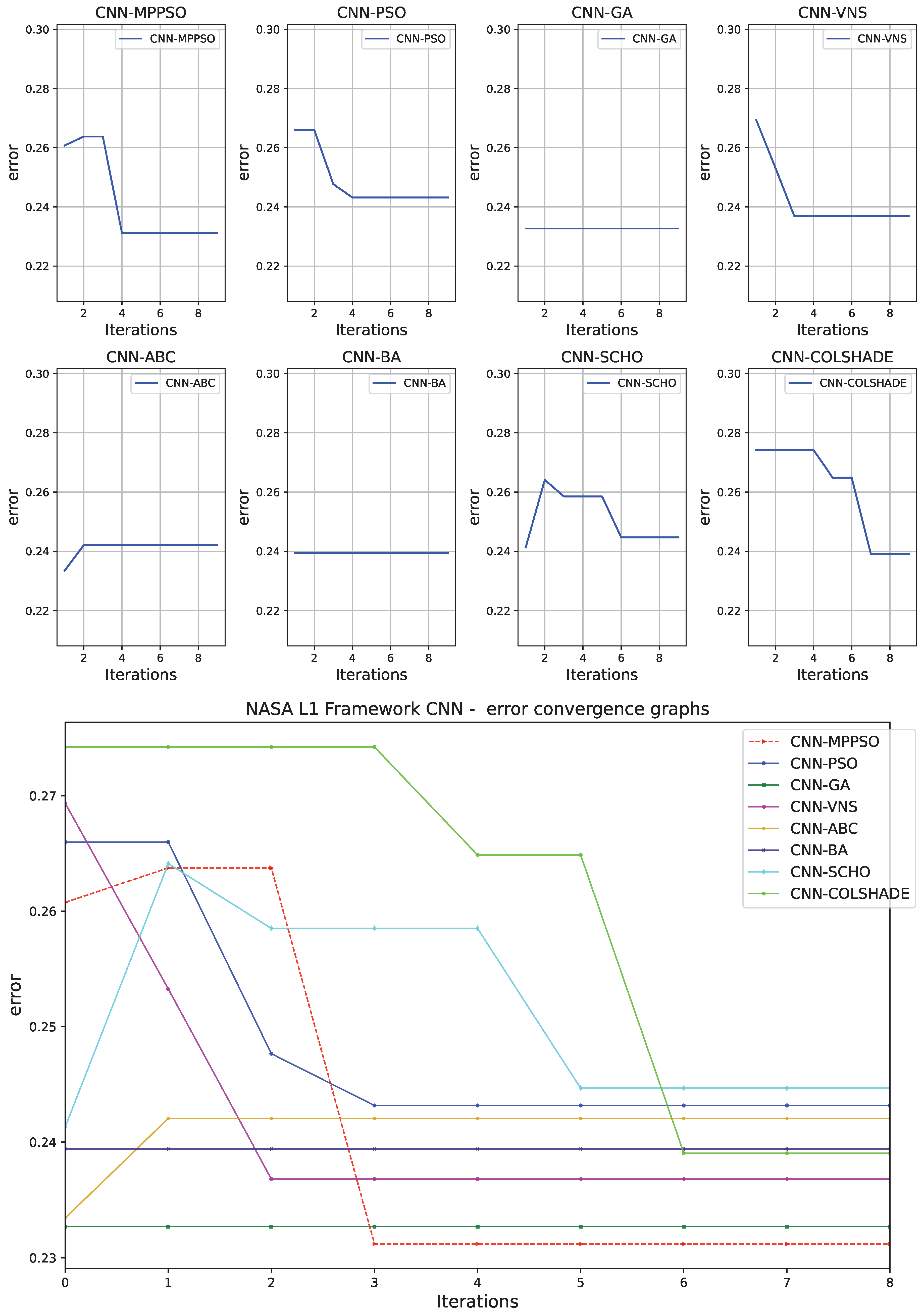
Figure 8.
CNN-MPPSO optimized L1 model ROC curve.
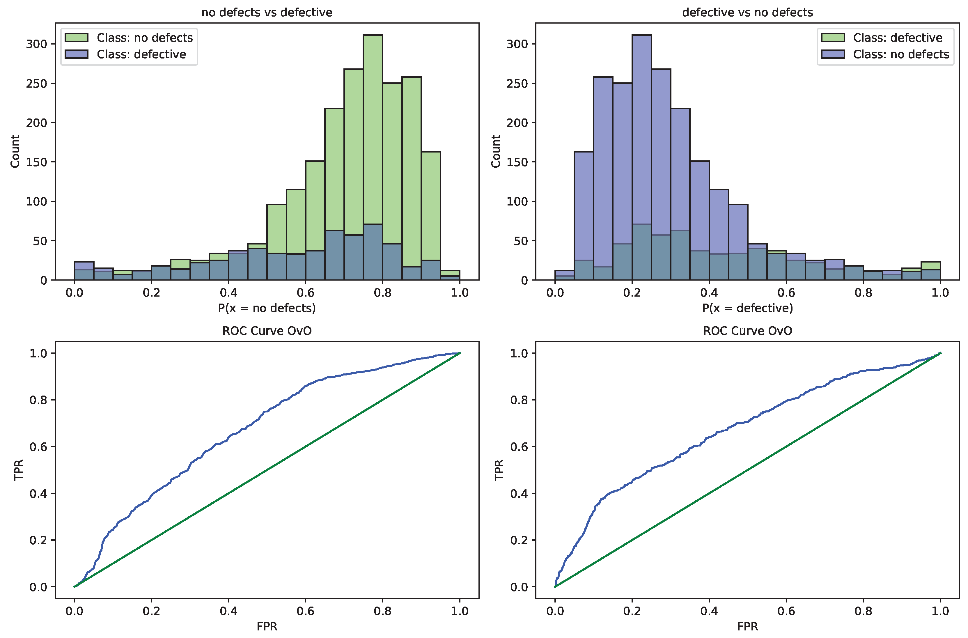
Figure 9.
CNN-MPPSO optimized L1 model confusion matrix.
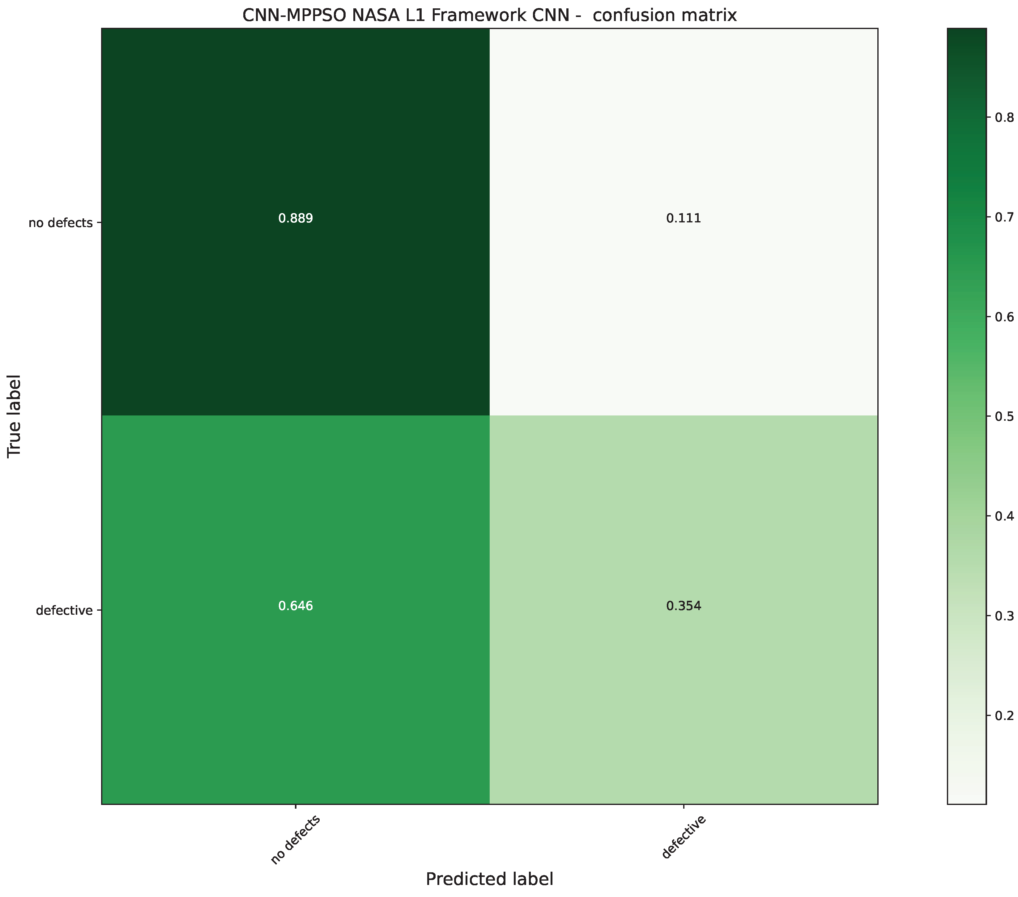
Figure 10.
Best CNN-MPPSO optimized L1 model visualization.
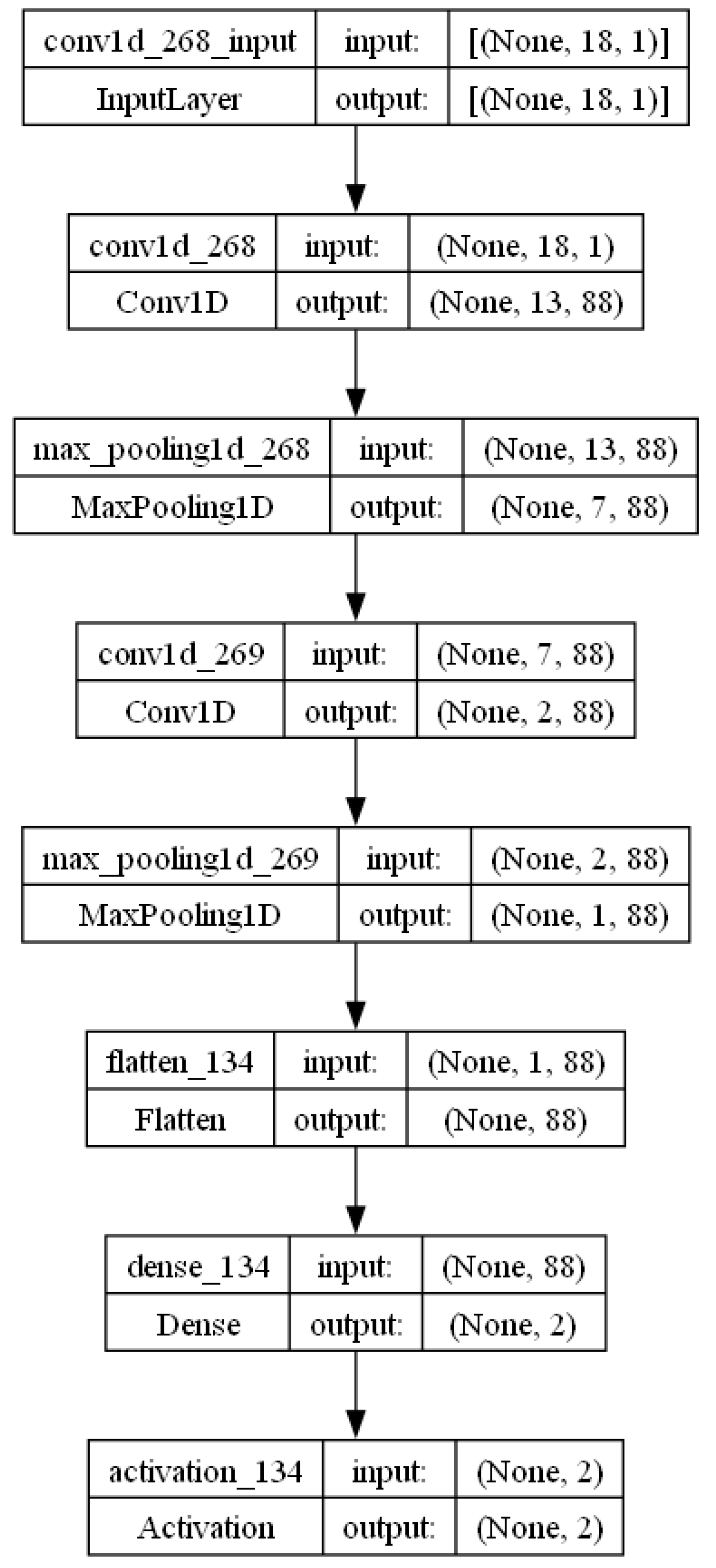
Figure 11.
Layer 2 AdaBoost objective and indicator outcome distributions.
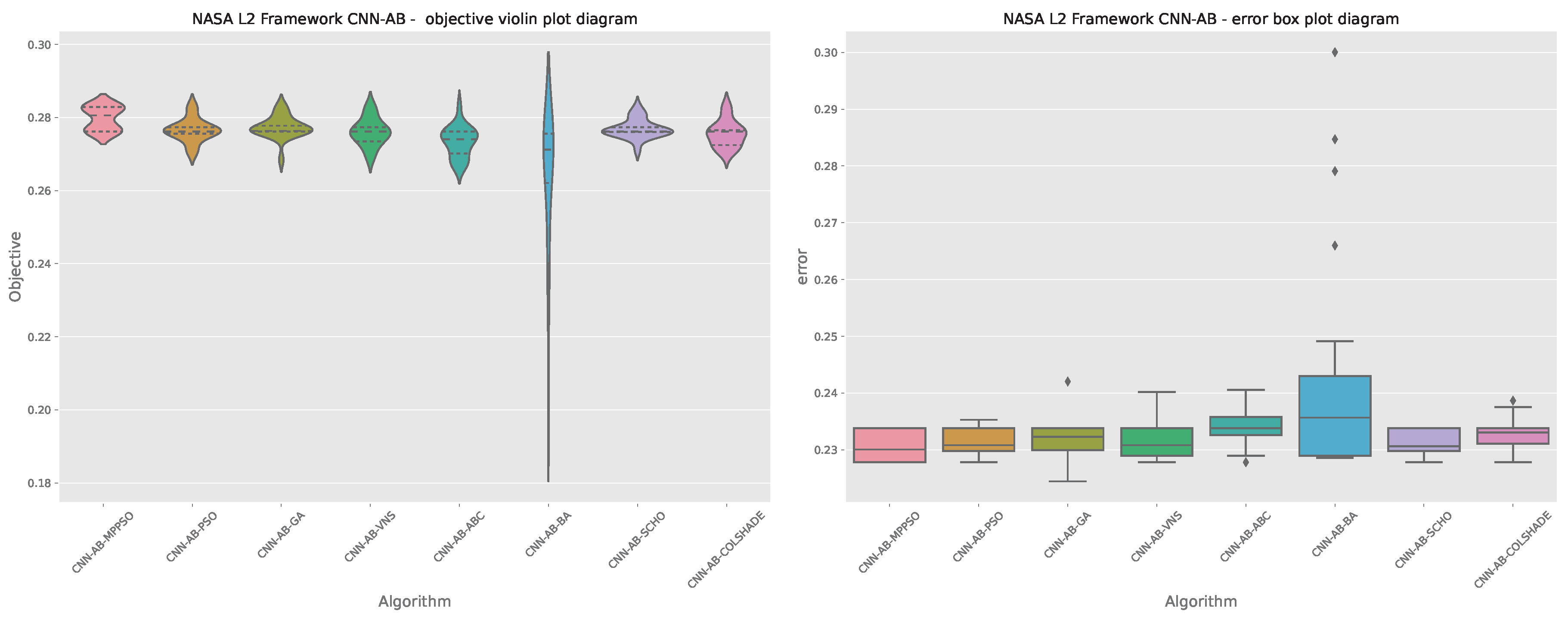
Figure 12.
Layer 2 AdaBoost objective function convergence.
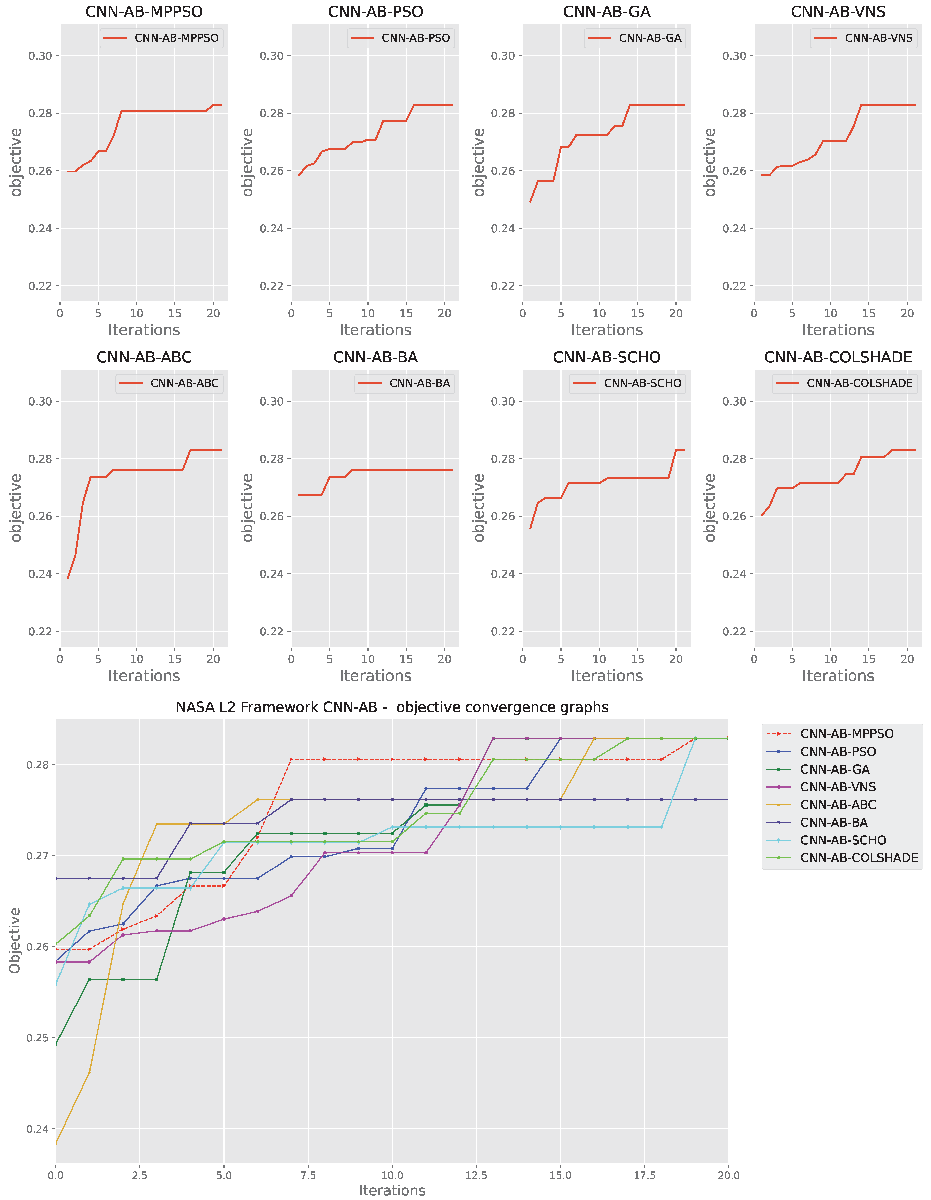
Figure 13.
Layer 2 AdaBoost indicator function convergence.
Figure 14.
Layer 2 AdaBoost optimized L1 model ROC curve.
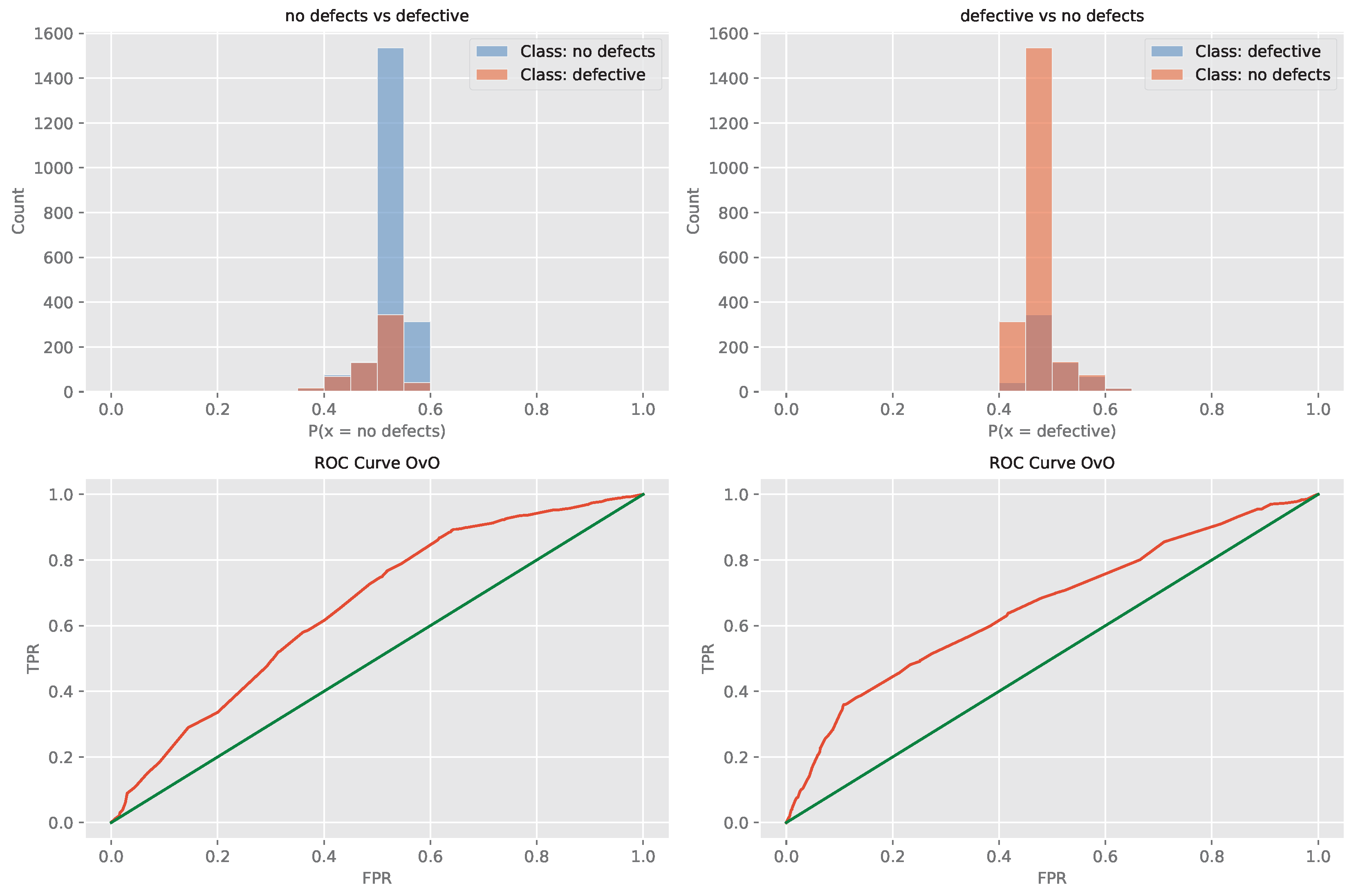
Figure 15.
Layer 2 AdaBoost optimized L1 model confusion matrix.
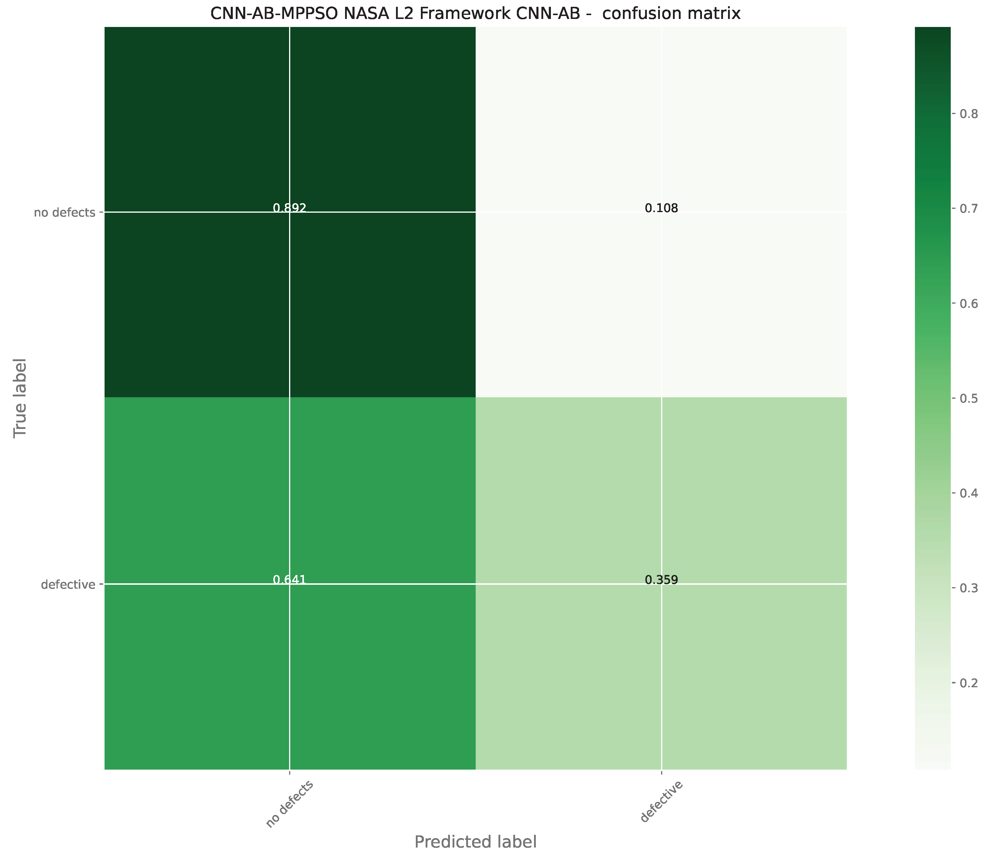
Figure 16.
Layer 2 XGBoost objective and indicator outcome distributions.
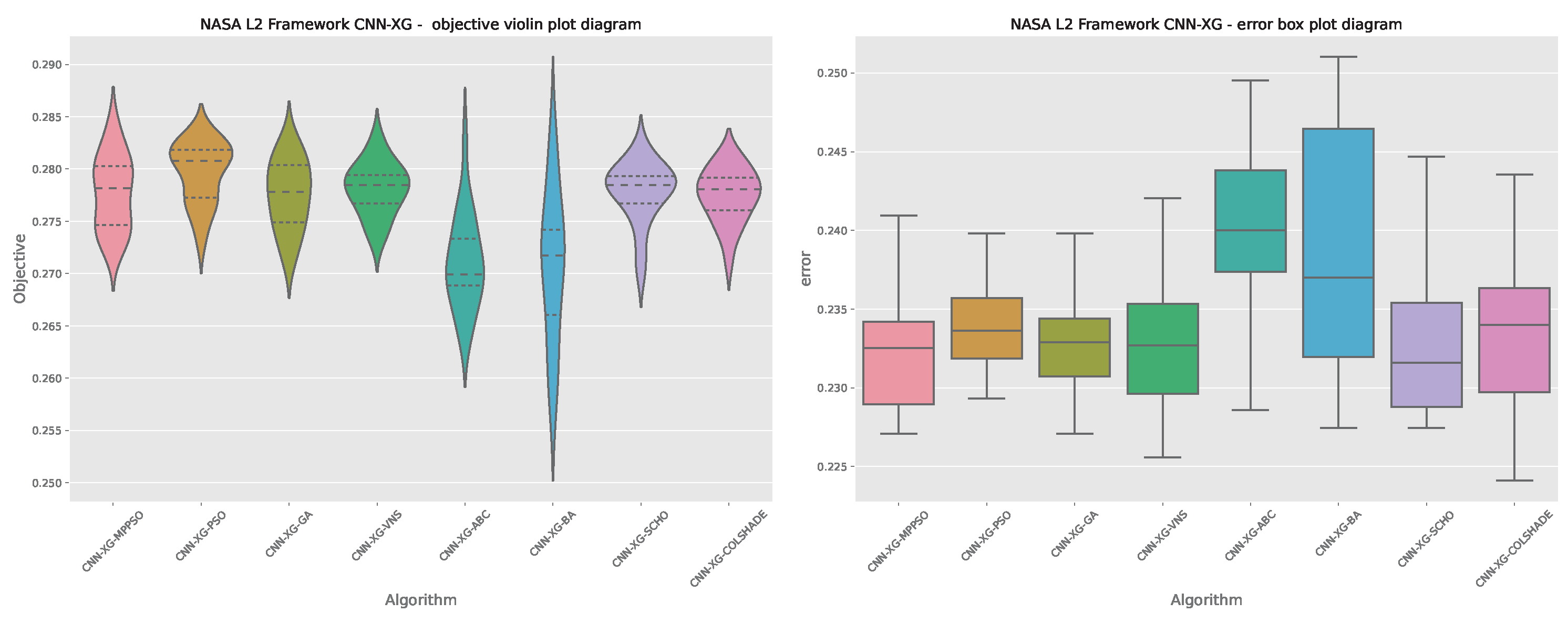
Figure 17.
Layer 2 XGBoost objective function convergence.
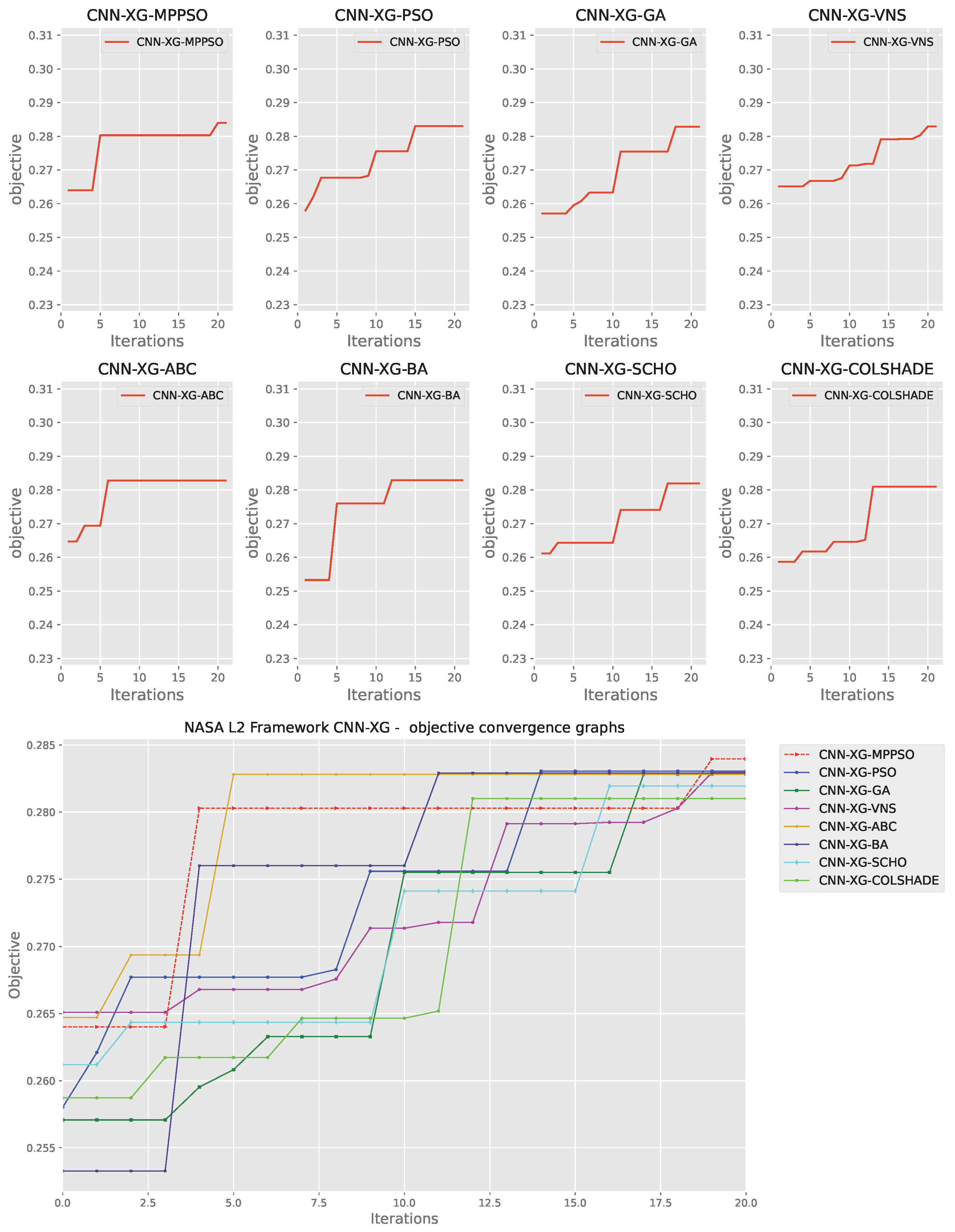
Figure 18.
Layer 2 XGBoost indicator function convergence.
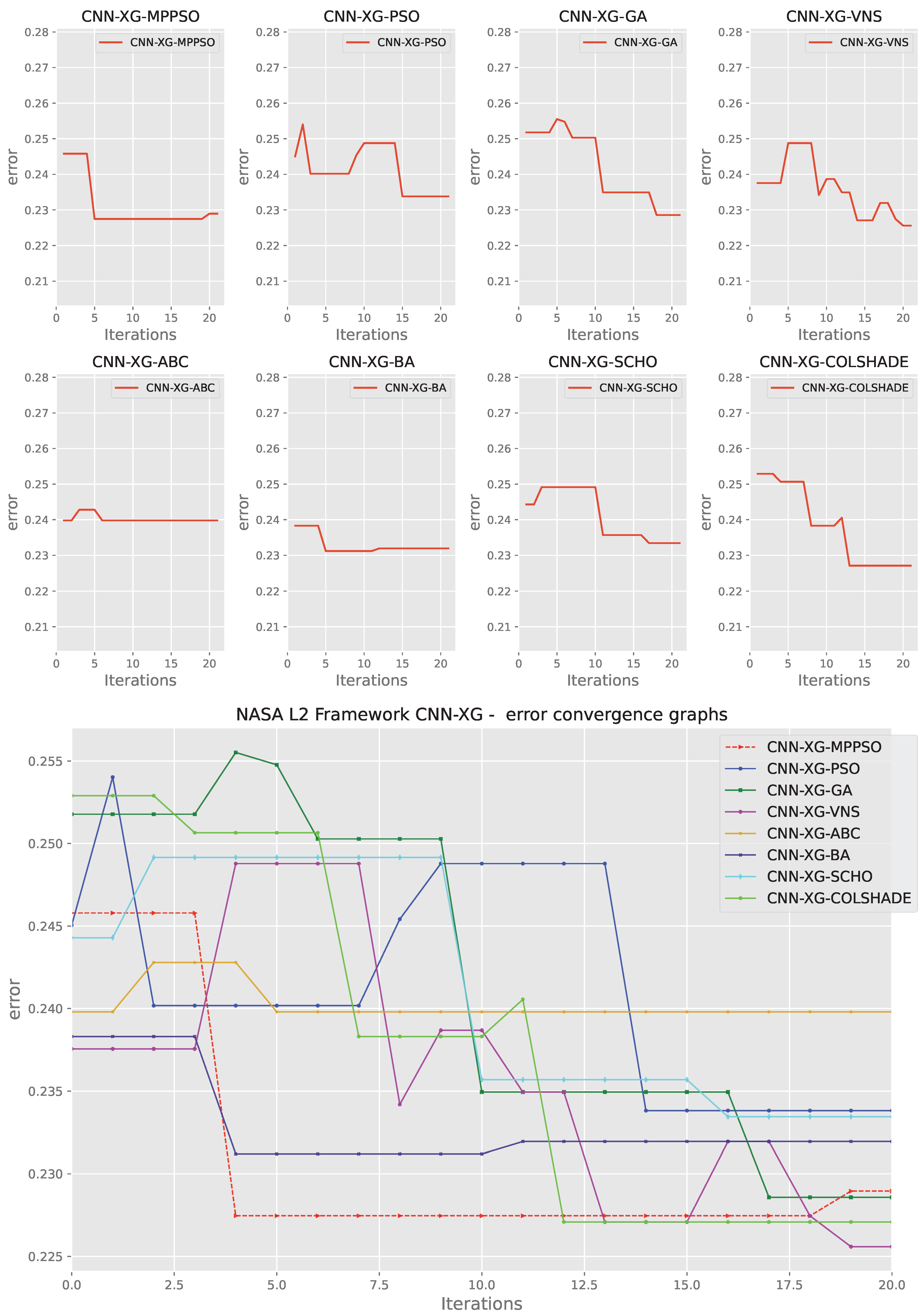
Figure 19.
Layer 2 XGBoost optimized L1 model ROC curve.
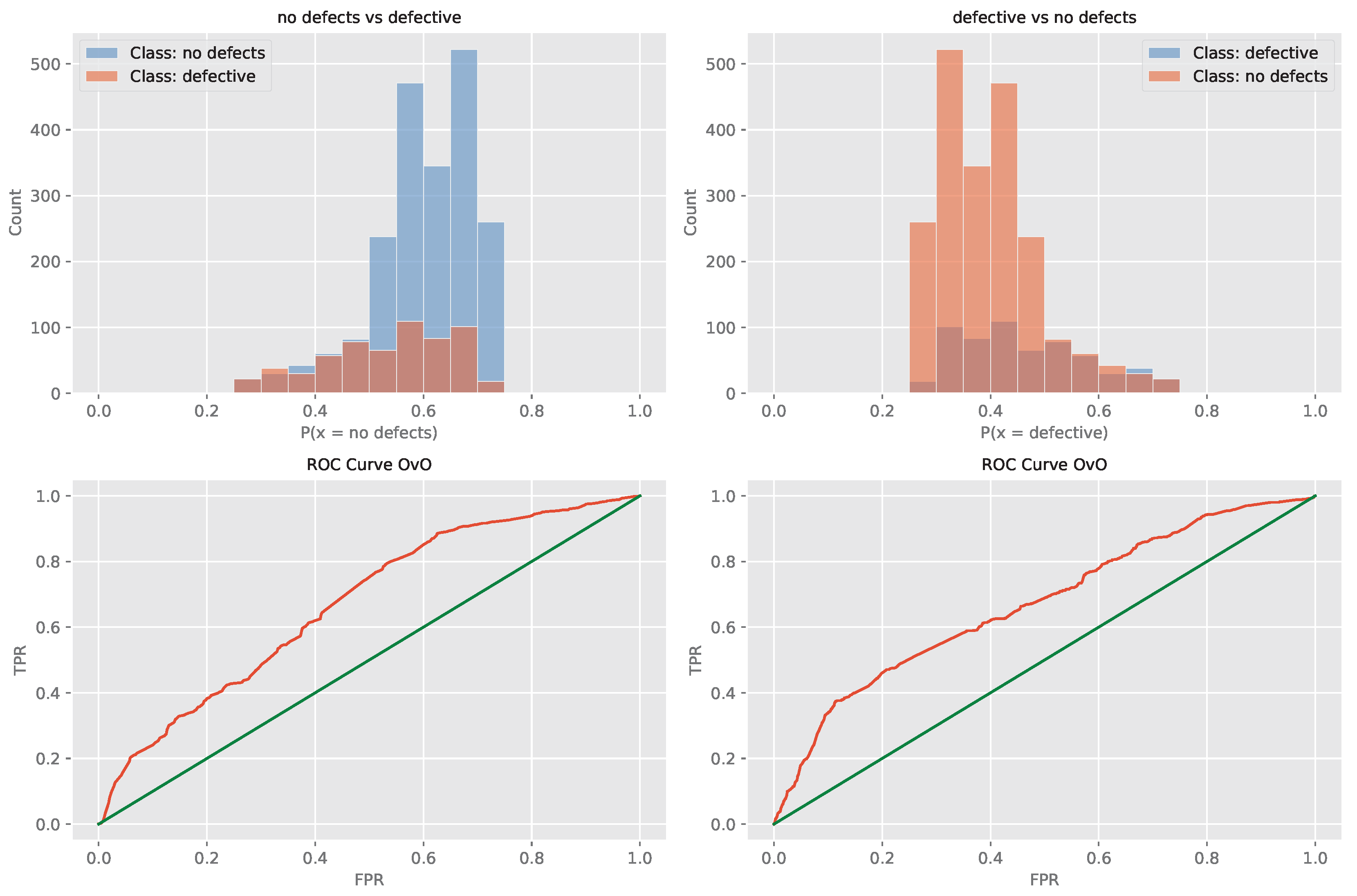
Figure 20.
Layer 2 XGBoost optimized L1 model confusion matrix.
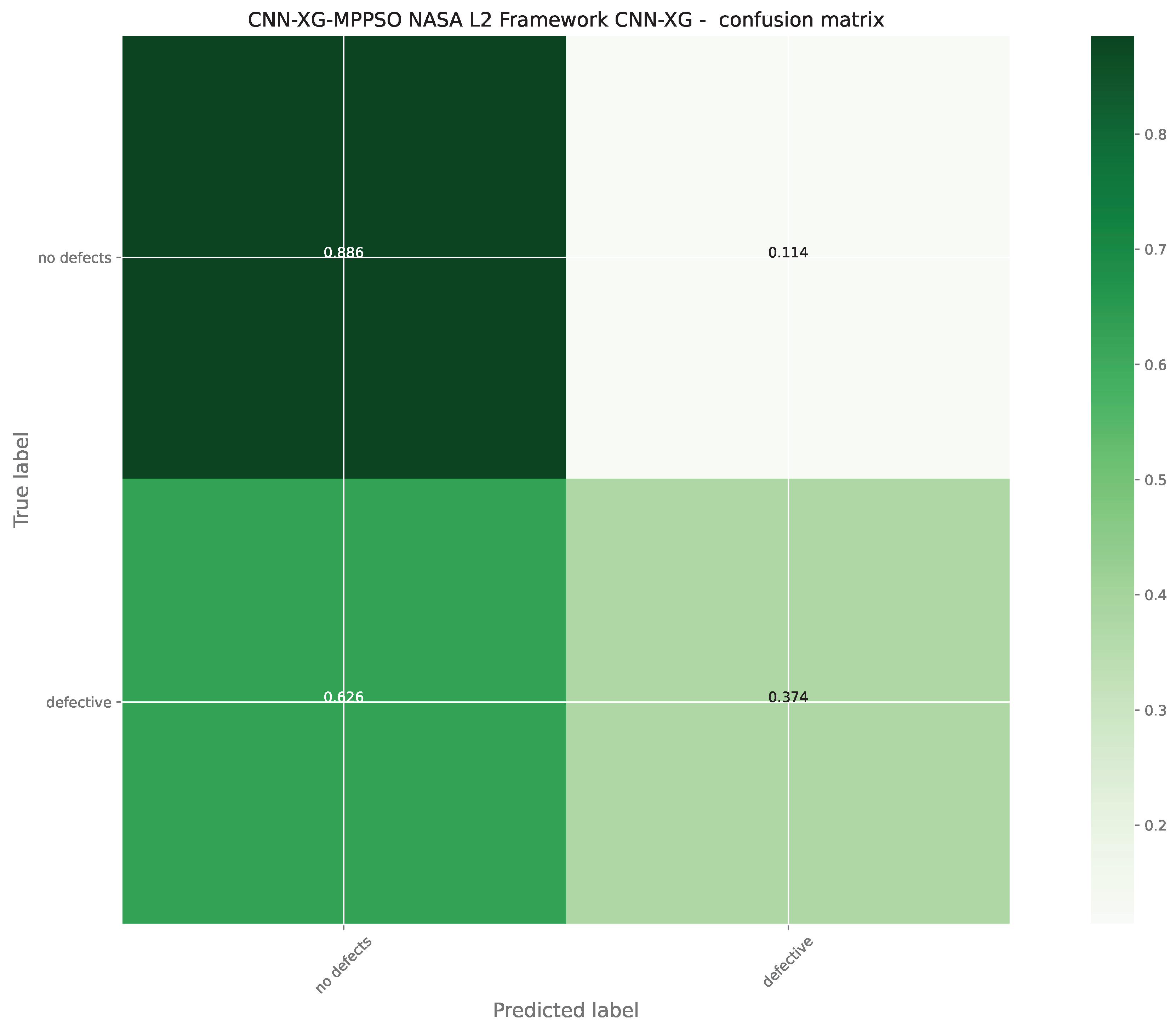
Figure 21.
NLP Layer 2 AdaBoost and indicator outcome distributions.
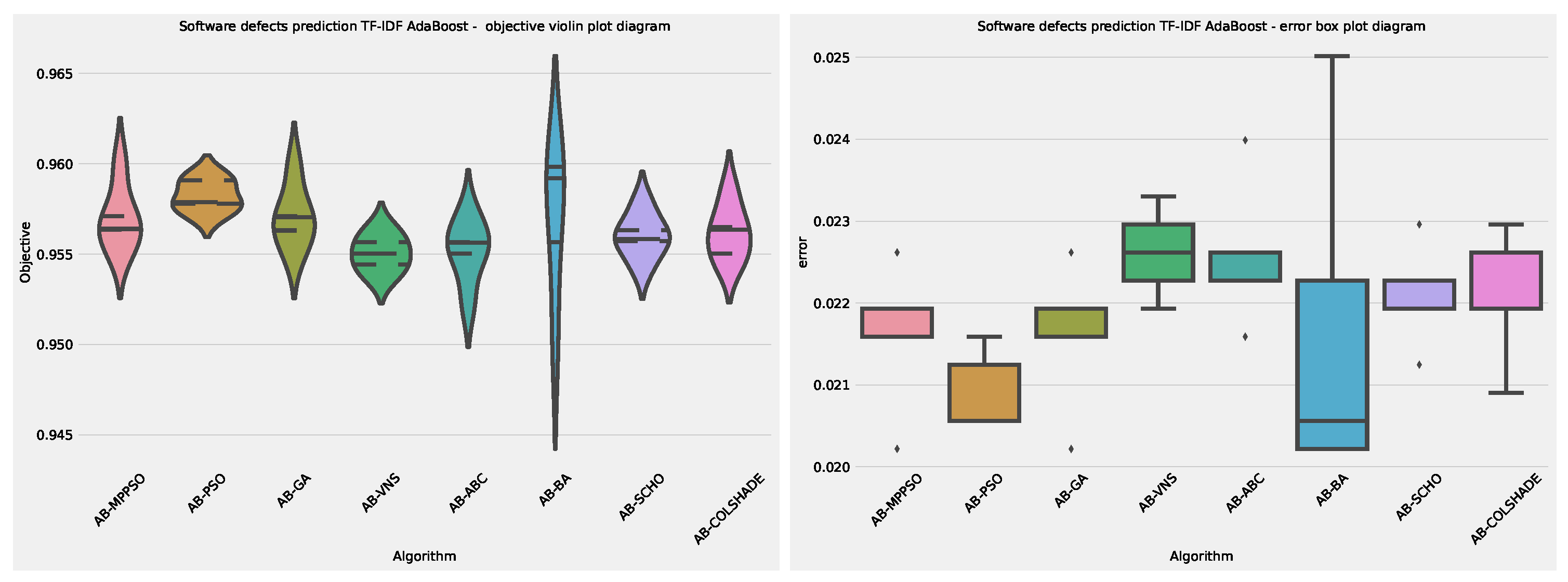
Figure 22.
NLP Layer 2 AdaBoost objective function convergence.
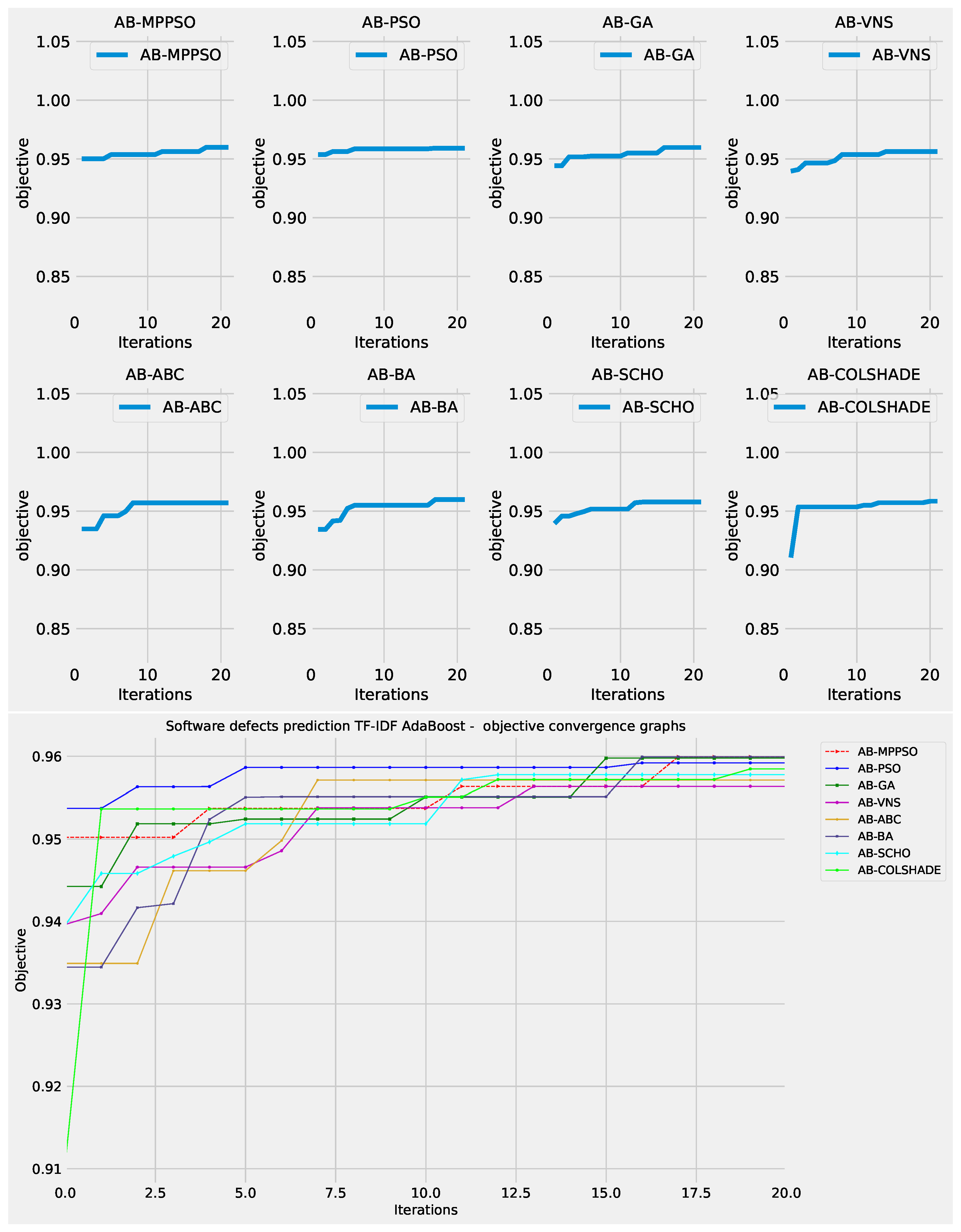
Figure 23.
NLP Layer 2 AdaBoost indicator function convergence.
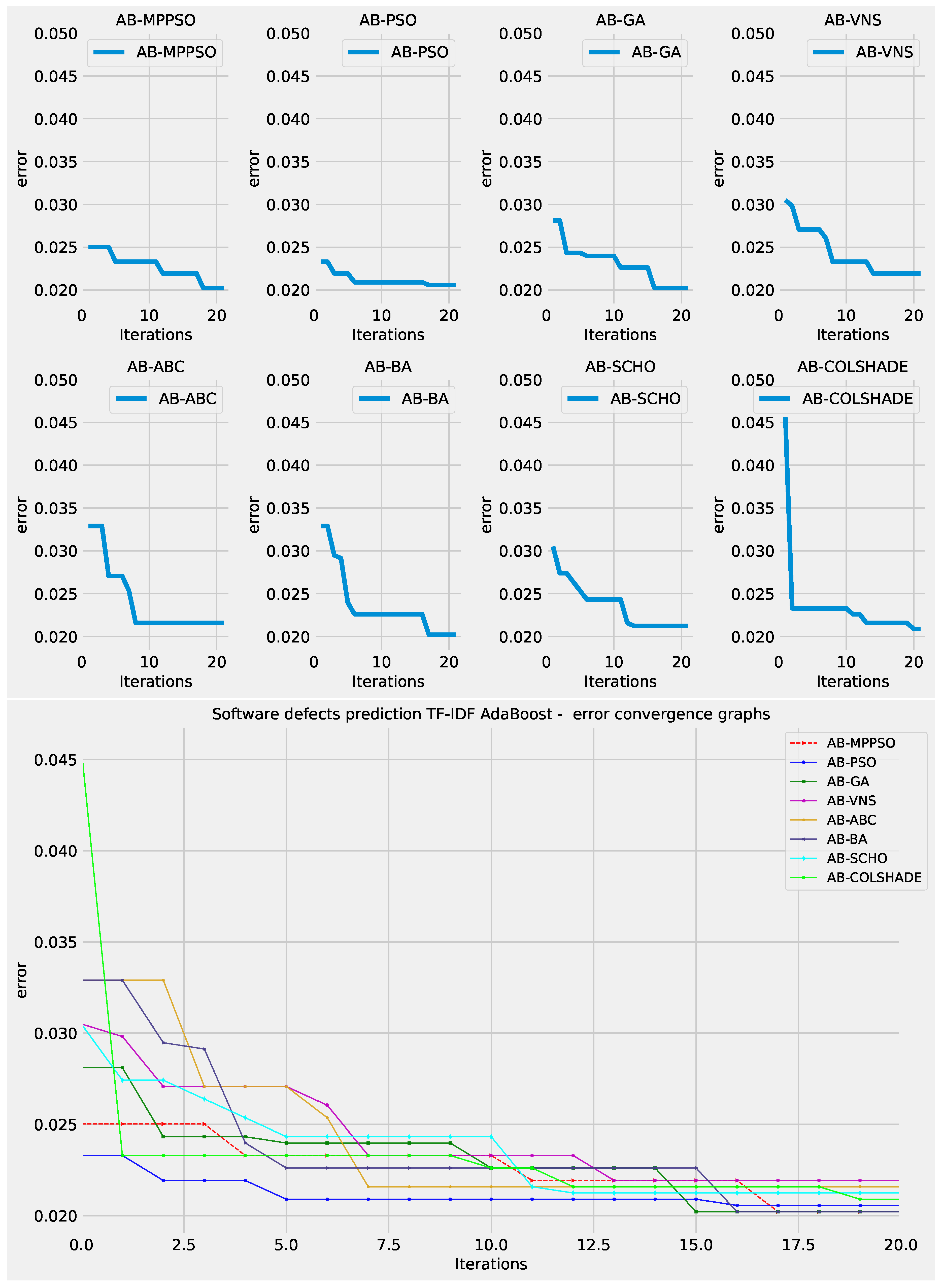
Figure 24.
NLP Layer 2 AdaBoost optimized model ROC curve.
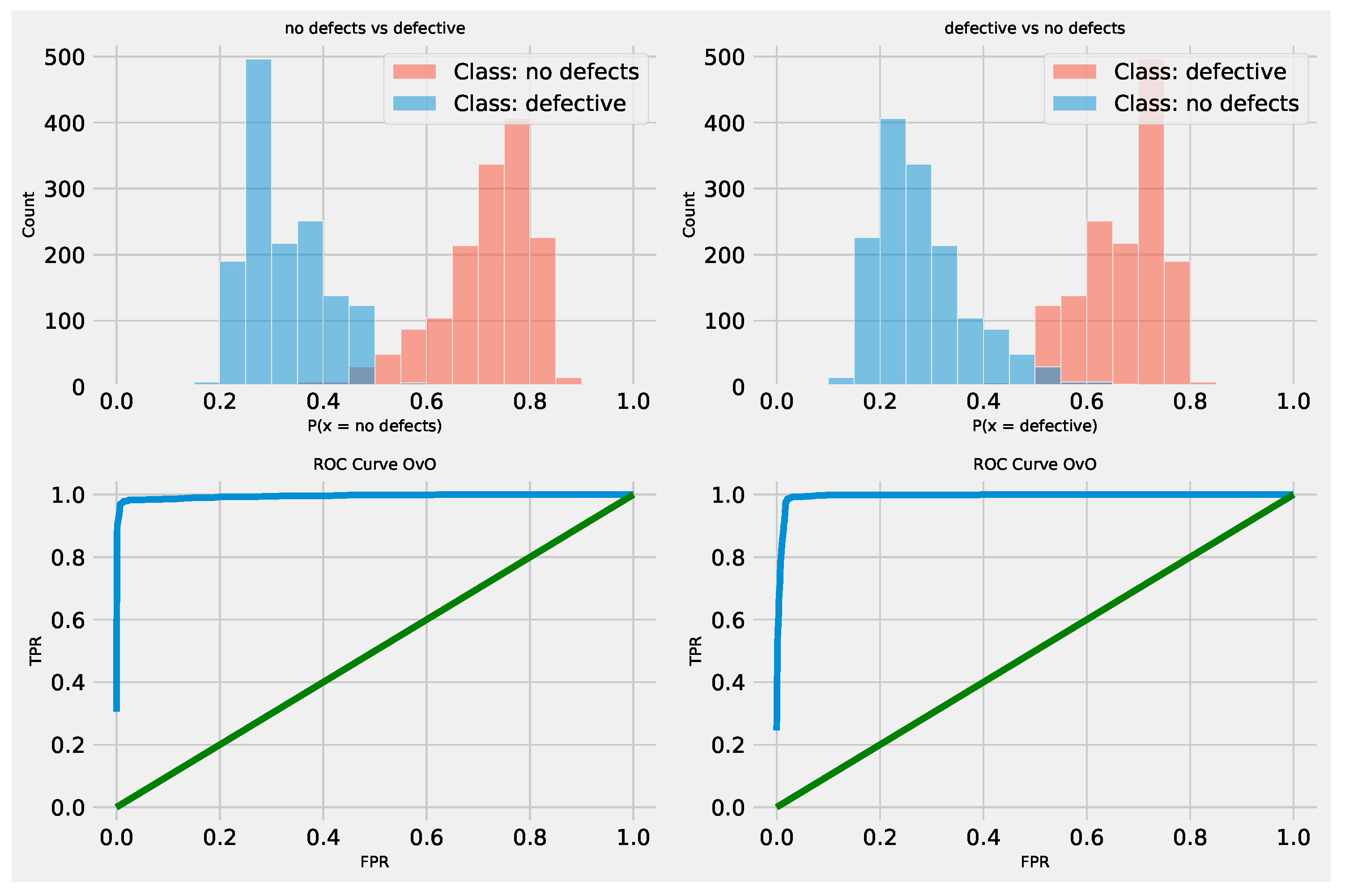
Figure 25.
NLP Layer 2 AdaBoost optimized model confusion matrix.
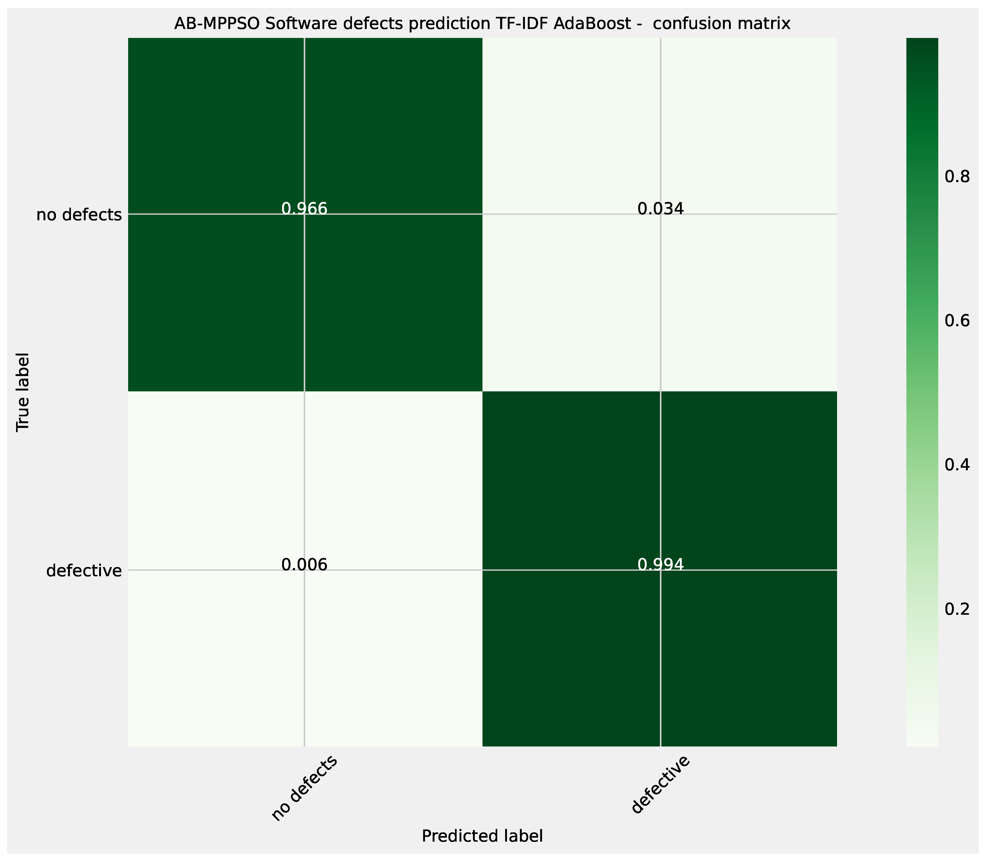
Figure 26.
NLP Layer 2 XGBoost and indicator outcome distributions.
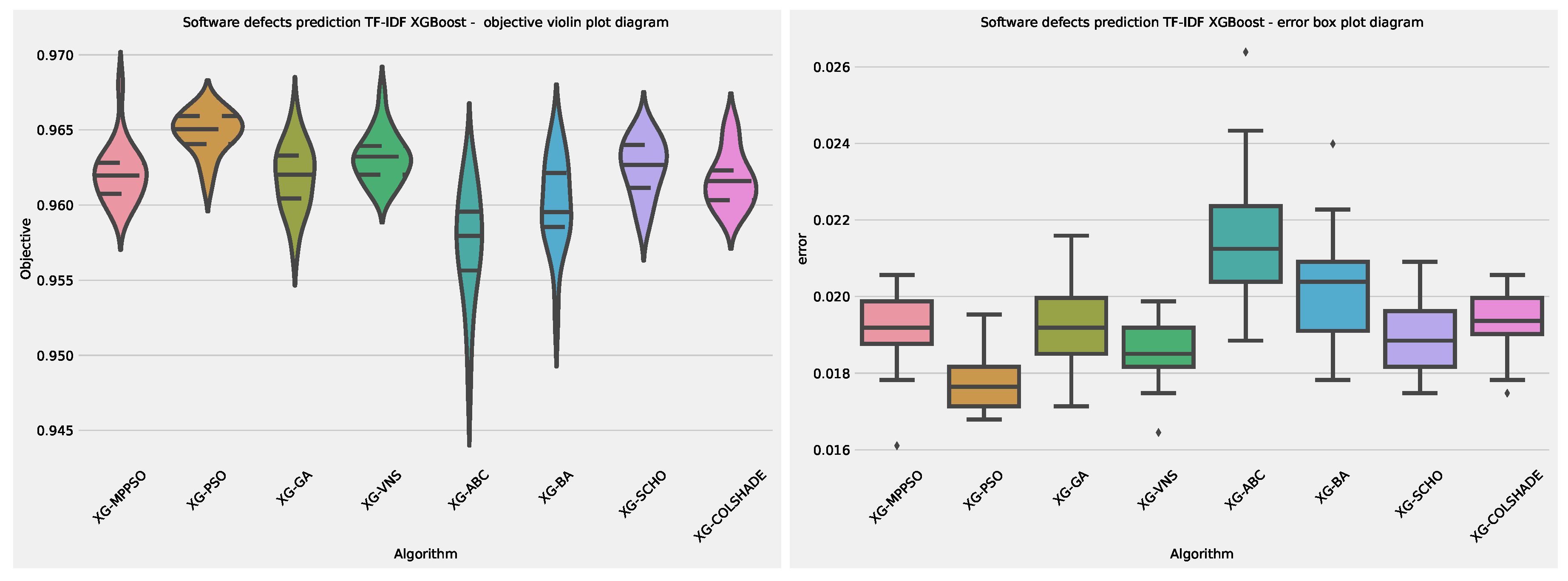
Figure 27.
NLP Layer 2 XGBoost objective function convergence.
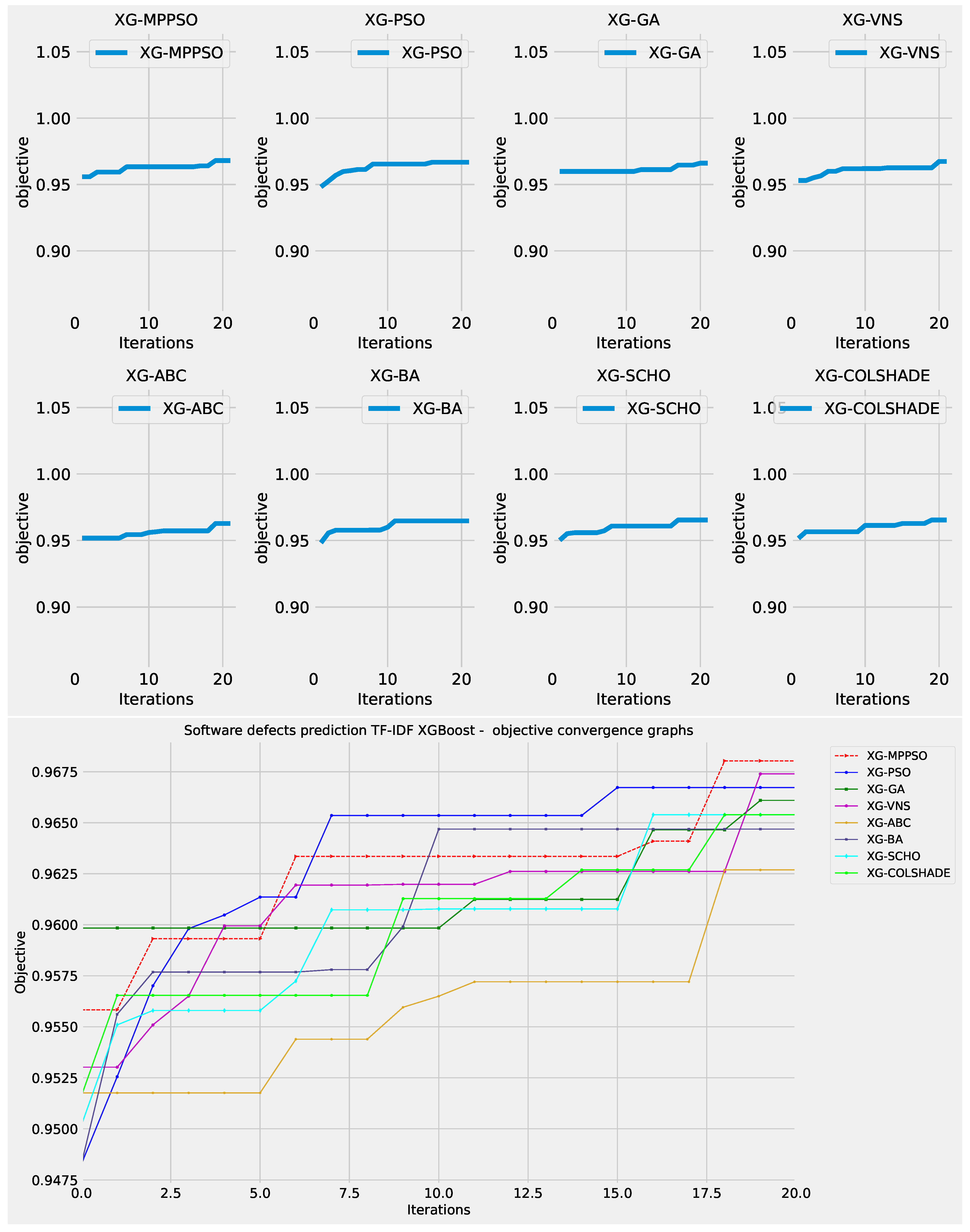
Figure 28.
NLP Layer 2 XGBoost indicator function convergence.
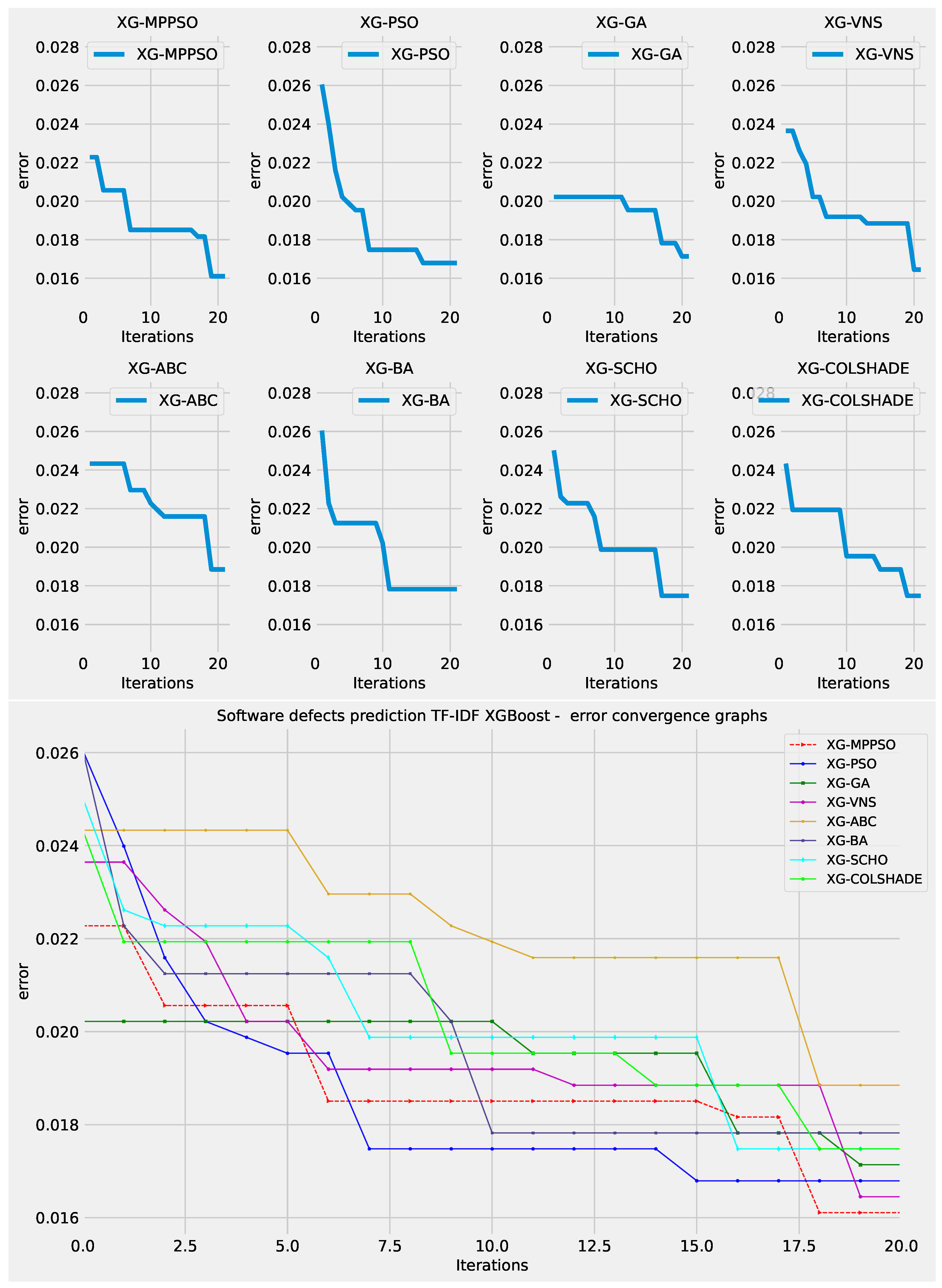
Figure 29.
NLP Layer 2 XGBoost optimized model ROC curve.
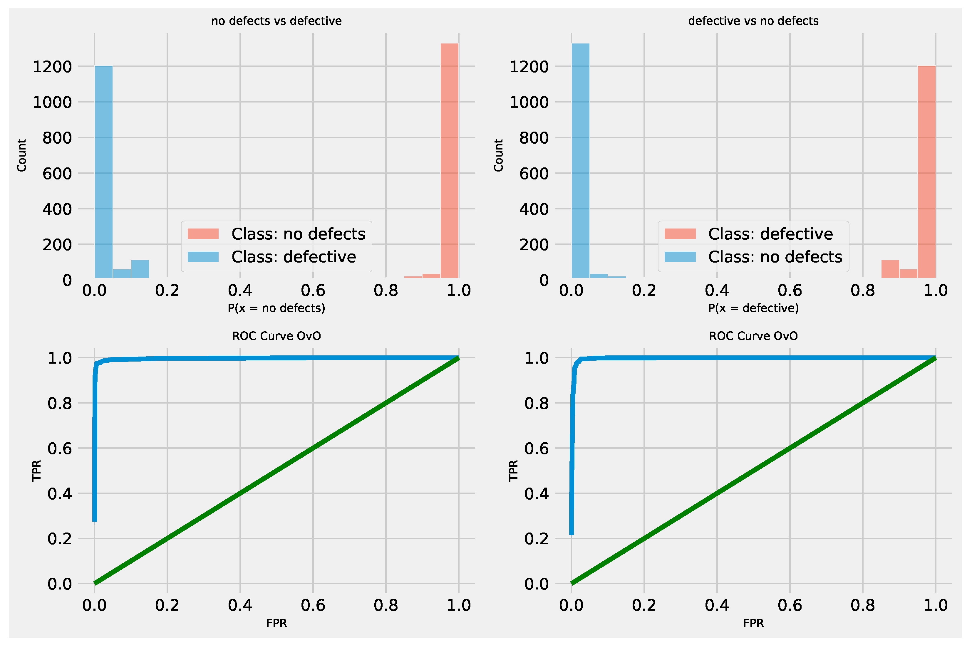
Figure 30.
NLP Layer 2 XGBoost optimized model confusion matrix.
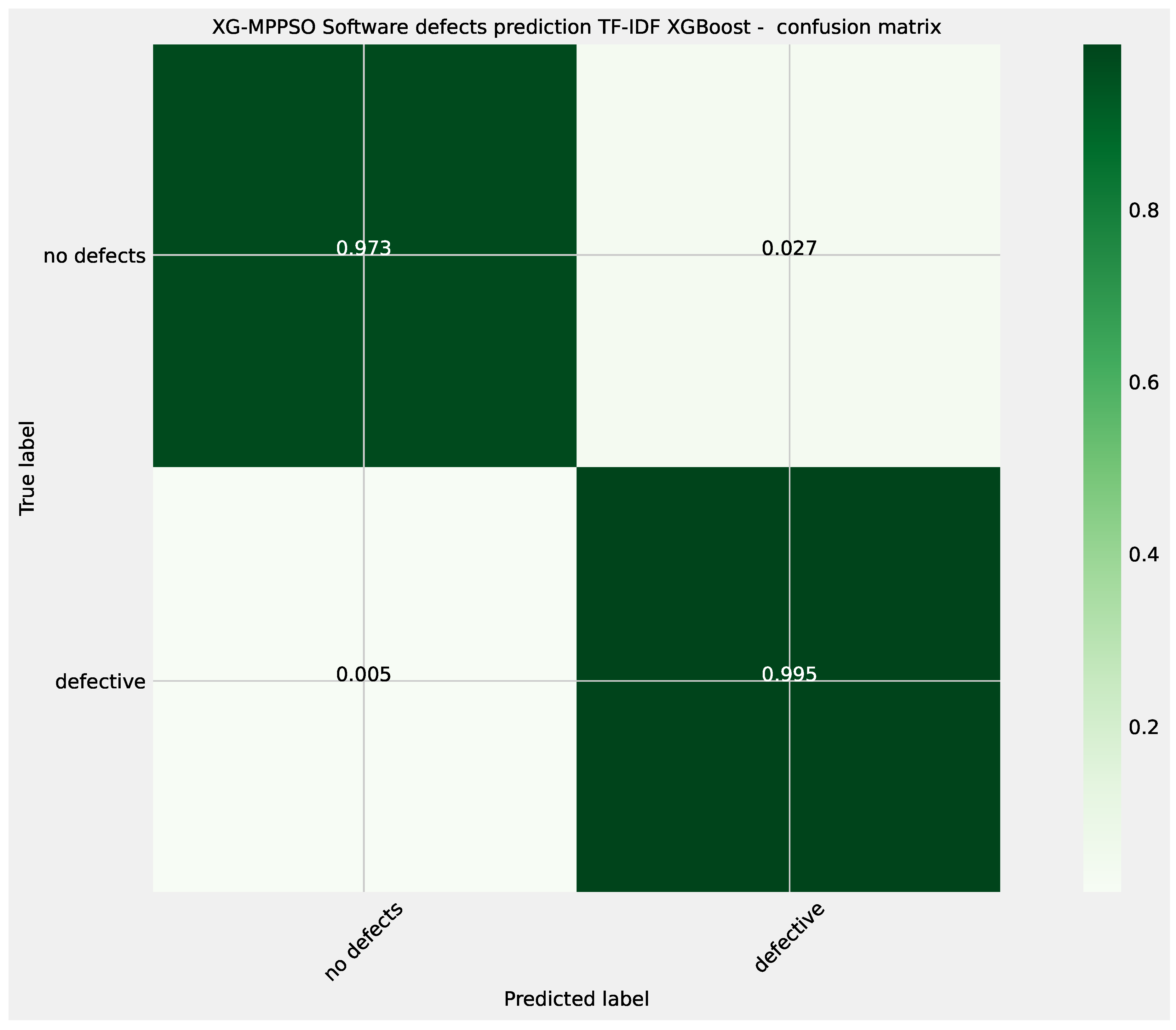
Figure 31.
KDE diagrams for all five conducted simulations.
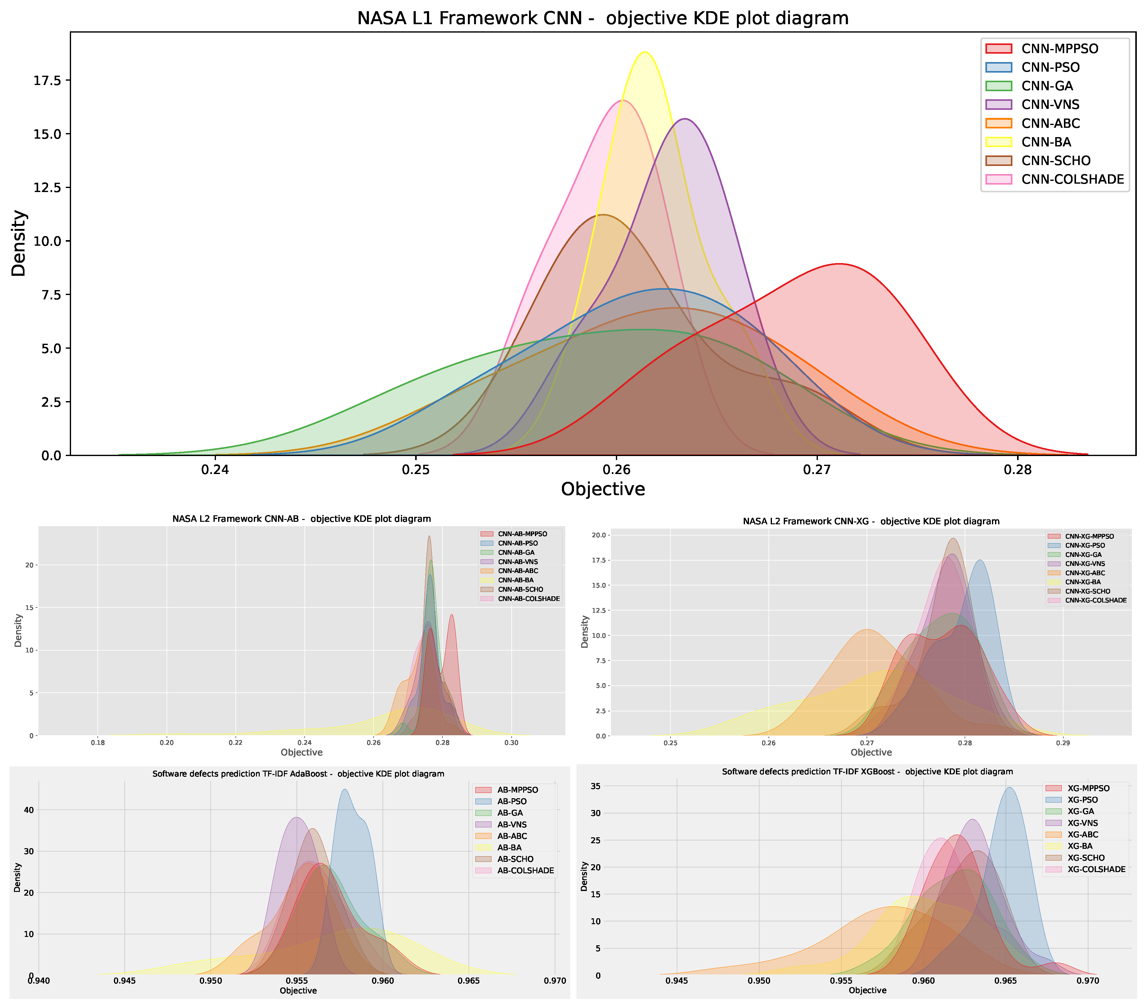
Figure 32.
Best CNN, XGBoost and AdaBoost model feature importances on NASA dataset.
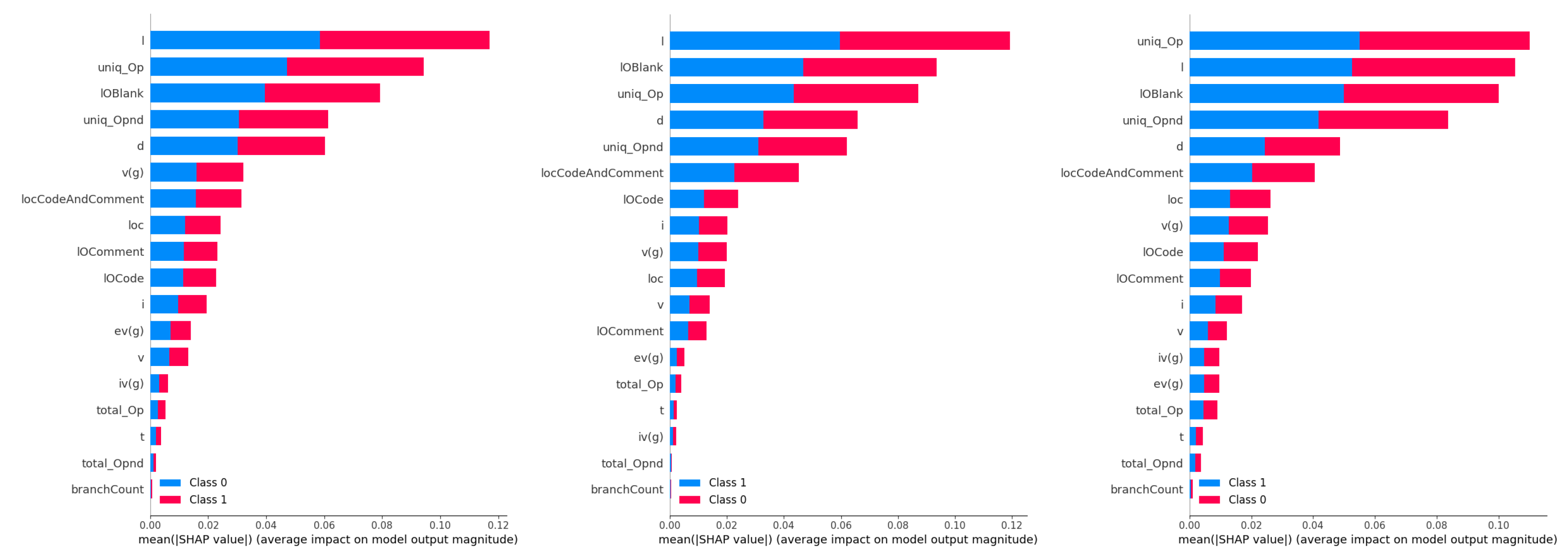
Figure 33.
Best AdaBoost model feature importances on NLP dataset.
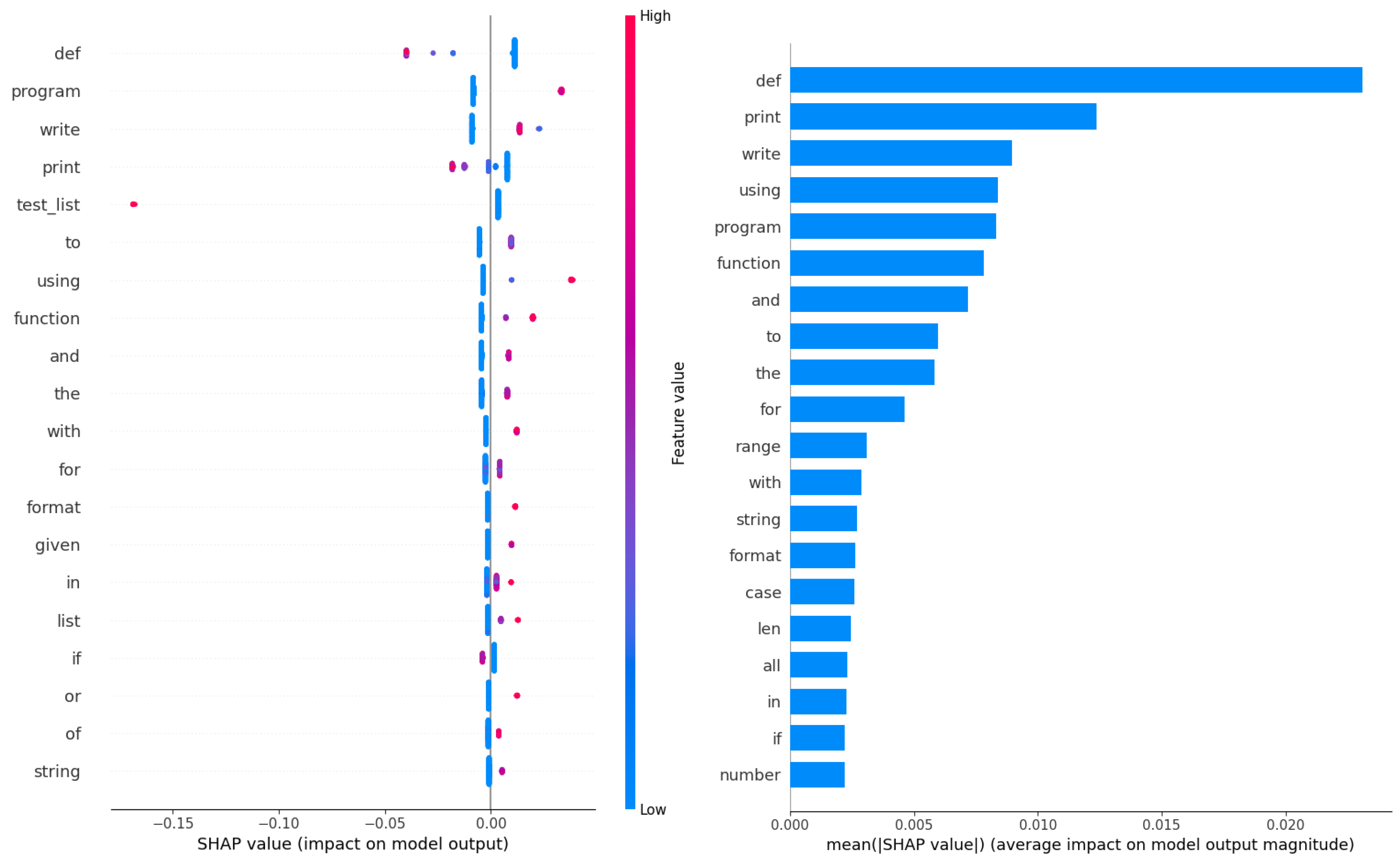
Figure 34.
Best XGBoost model feature importance’s on NLP dataset.
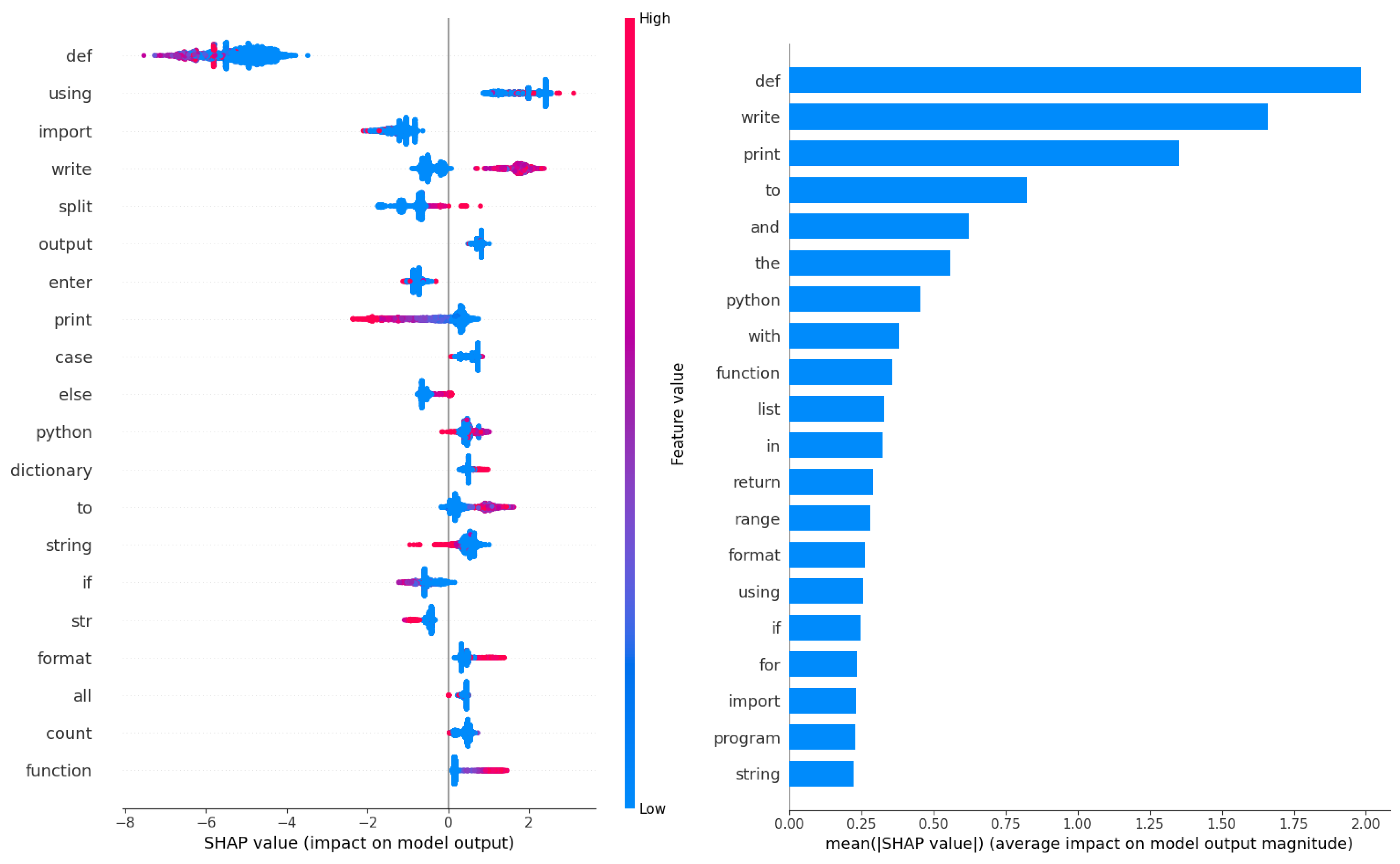

Table 1.
CNN parameter ranges subjected to optimization.
| Parameter | Range |
|---|---|
| Learning Rate | 0.0001 - 0.0030 |
| Dropout | 0.05 - 0.5 |
| Epochs | 10 - 20 |
| Number of CNN Layers | 1 - 3 |
| Number of Dense Layers | 1 - 3 |
| Number of Neurons in layer | 32 - 128 |
Table 2.
AdaBoost parameter ranges subjected to optimization.
| Parameter | Range |
|---|---|
| Count of estimators | |
| Depth | |
| Learning rate |
Table 3.
XGBoost parameter ranges subjected to optimization.
| Parameter | Range |
|---|---|
| Learning Rate | 0.1 - 0.9 |
| Minimum child weight | 1 - 10 |
| Subsample | 0.01 - 1.00 |
| Col sample by tree | 0.01 - 1.00 |
| Max depth | 3 - 10 |
| Gamma | 0.00 - 0.80 |
Table 4.
Layer 1 (CNN) objective function outcomes.
| Method | Best | Worst | Mean | Median | Std | Var |
|---|---|---|---|---|---|---|
| CNN-MPPSO | 0.273280 | 0.262061 | 0.268824 | 0.269873 | 0.004194 | 1.76E-05 |
| CNN-PSO | 0.267168 | 0.253372 | 0.261106 | 0.260917 | 0.004766 | 2.27E-05 |
| CNN-GA | 0.265933 | 0.249726 | 0.258941 | 0.258989 | 0.005977 | 3.57E-05 |
| CNN-VNS | 0.265920 | 0.258217 | 0.262605 | 0.263118 | 0.002553 | 6.52E-06 |
| CNN-ABC | 0.269294 | 0.253197 | 0.261761 | 0.262521 | 0.005419 | 2.94E-05 |
| CNN-BA | 0.265823 | 0.258906 | 0.261940 | 0.261646 | 0.002218 | 4.92E-06 |
| CNN-SCHO | 0.268643 | 0.257094 | 0.261124 | 0.259722 | 0.003986 | 1.59E-05 |
| CNN-COLSHADE | 0.262284 | 0.255697 | 0.259373 | 0.260087 | 0.002277 | 5.18E-06 |
Table 5.
Layer 1 (CNN) indicator function outcomes.
| Method | Best | Worst | Mean | Median | Std | Var |
|---|---|---|---|---|---|---|
| CNN-MPPSO | 0.231201 | 0.238309 | 0.233446 | 0.232697 | 0.002810 | 7.89E-06 |
| CNN-PSO | 0.243172 | 0.267116 | 0.248784 | 0.243172 | 0.012645 | 1.60E-04 |
| CNN-GA | 0.232697 | 0.260756 | 0.252450 | 0.260756 | 0.015398 | 2.37E-04 |
| CNN-VNS | 0.236813 | 0.239805 | 0.237710 | 0.236813 | 0.005652 | 3.19E-05 |
| CNN-ABC | 0.242050 | 0.242798 | 0.244444 | 0.242050 | 0.007371 | 5.43E-05 |
| CNN-BA | 0.239431 | 0.230079 | 0.238608 | 0.237561 | 0.006460 | 4.17E-05 |
| CNN-SCHO | 0.244669 | 0.263749 | 0.249532 | 0.244669 | 0.009629 | 9.27E-05 |
| CNN-COLSHADE | 0.239057 | 0.244669 | 0.245866 | 0.244669 | 0.007860 | 6.18E-05 |
Table 6.
Best performing optimized CNN-MPPSO L1 model detailed metric comparisons.
| Method | metric | no error | error | accuracy | macro avg | weighted avg |
|---|---|---|---|---|---|---|
| CNN- | precision | 0.826009 | 0.480813 | 0.768799 | 0.653411 | 0.748395 |
| MPPSO | recall | 0.888996 | 0.354409 | 0.768799 | 0.621703 | 0.768799 |
| f1-score | 0.856346 | 0.408046 | 0.768799 | 0.632196 | 0.755550 | |
| CNN- | precision | 0.829777 | 0.452611 | 0.756828 | 0.641194 | 0.744975 |
| PSO | recall | 0.863417 | 0.389351 | 0.756828 | 0.626384 | 0.756828 |
| f1-score | 0.846263 | 0.418605 | 0.756828 | 0.632434 | 0.750108 | |
| CNN- | precision | 0.768653 | 0.188725 | 0.680135 | 0.478689 | 0.638262 |
| GA | recall | 0.840251 | 0.128120 | 0.680135 | 0.484185 | 0.680135 |
| f1-score | 0.802859 | 0.152626 | 0.680135 | 0.477743 | 0.656660 | |
| CNN- | precision | 0.826304 | 0.465812 | 0.763187 | 0.646058 | 0.745250 |
| VNS | recall | 0.879344 | 0.362729 | 0.763187 | 0.621036 | 0.763187 |
| f1-score | 0.851999 | 0.407858 | 0.763187 | 0.629928 | 0.752138 | |
| CNN- | precision | 0.830014 | 0.455253 | 0.757950 | 0.642633 | 0.745752 |
| ABC | recall | 0.864865 | 0.389351 | 0.757950 | 0.627108 | 0.757950 |
| f1-score | 0.847081 | 0.419731 | 0.757950 | 0.633406 | 0.750995 | |
| CNN- | precision | 0.827539 | 0.459959 | 0.760569 | 0.643749 | 0.744892 |
| BA | recall | 0.873069 | 0.372712 | 0.760569 | 0.622891 | 0.760569 |
| f1-score | 0.849695 | 0.411765 | 0.760569 | 0.630730 | 0.751230 | |
| CNN- | precision | 0.830999 | 0.450094 | 0.755331 | 0.640547 | 0.745356 |
| SCHO | recall | 0.859073 | 0.397671 | 0.755331 | 0.628372 | 0.755331 |
| f1-score | 0.844803 | 0.422261 | 0.755331 | 0.633532 | 0.749798 | |
| CNN- | precision | 0.826127 | 0.460084 | 0.760943 | 0.643105 | 0.743825 |
| COLSHADE | recall | 0.875965 | 0.364393 | 0.760943 | 0.620179 | 0.760943 |
| f1-score | 0.850316 | 0.406685 | 0.760943 | 0.628501 | 0.750570 | |
| support | 2072 | 601 |
Table 7.
Optimized CNN model parameter selections.
| Method | Learning | Dropout | Epochs | Layers | Layers | Neurons | Neurons |
|---|---|---|---|---|---|---|---|
| Rate | CNN | Dense | CNN | Dense | |||
| CNN-MPPSO | 2.44E-03 | 0.500000 | 84 | 1.0 | 1.0 | 88 | 88 |
| CNN-PSO | 2.80E-03 | 0.165591 | 56 | 1.0 | 1.0 | 97 | 83 |
| CNN-GA | 1.66E-03 | 0.475371 | 65 | 1.0 | 1.0 | 94 | 86 |
| CNN-VNS | 2.38E-03 | 0.500000 | 42 | 1.0 | 1.0 | 128 | 93 |
| CNN-ABC | 2.61E-03 | 0.370234 | 93 | 2.0 | 1.0 | 124 | 96 |
| CNN-BA | 3.00E-03 | 0.500000 | 70 | 2.0 | 2.0 | 108 | 103 |
| CNN-SCHO | 1.25E-03 | 0.197273 | 100 | 1.0 | 2.0 | 46 | 105 |
| CNN-COLSHADE | 1.88E-03 | 0.230465 | 86 | 2.0 | 2.0 | 73 | 99 |
Table 8.
Layer 2 AdaBoost objective function outcomes.
| Method | Best | Worst | Mean | Median | Std | Var |
|---|---|---|---|---|---|---|
| CNN-AB-MPPSO | 0.282906 | 0.276185 | 0.279771 | 0.280600 | 0.003092 | 9.56E-06 |
| CNN-AB-PSO | 0.282906 | 0.270598 | 0.276496 | 0.276185 | 0.003085 | 9.51E-06 |
| CNN-AB-GA | 0.282906 | 0.268442 | 0.277295 | 0.276351 | 0.002980 | 8.88E-06 |
| CNN-AB-VNS | 0.282906 | 0.269109 | 0.276079 | 0.276185 | 0.003662 | 1.34E-05 |
| CNN-AB-ABC | 0.282906 | 0.266412 | 0.273352 | 0.274076 | 0.004034 | 1.63E-05 |
| CNN-AB-BA | 0.276185 | 0.202141 | 0.262977 | 0.271189 | 0.019258 | 3.71E-04 |
| CNN-AB-SCHO | 0.282906 | 0.271101 | 0.276876 | 0.276185 | 0.002530 | 6.40E-06 |
| CNN-AB-COLSHADE | 0.282906 | 0.270156 | 0.275568 | 0.276185 | 0.003515 | 1.24E-05 |
Table 9.
Layer 2 AdaBoost objective function outcomes.
| Method | Best | Worst | Mean | Median | Std | Var |
|---|---|---|---|---|---|---|
| CNN-AB-MPPSO | 0.227834 | 0.233820 | 0.230453 | 0.230079 | 0.002661 | 7.08E-06 |
| CNN-AB-PSO | 0.227834 | 0.228208 | 0.231481 | 0.230827 | 0.002380 | 5.67E-06 |
| CNN-AB-GA | 0.227834 | 0.242050 | 0.231874 | 0.232323 | 0.003529 | 1.25E-05 |
| CNN-AB-VNS | 0.227834 | 0.239057 | 0.232080 | 0.230827 | 0.003587 | 1.29E-05 |
| CNN-AB-ABC | 0.227834 | 0.235316 | 0.234287 | 0.233820 | 0.003431 | 1.18E-05 |
| CNN-AB-BA | 0.233820 | 0.249158 | 0.244239 | 0.235690 | 0.020533 | 4.22E-04 |
| CNN-AB-SCHO | 0.227834 | 0.233446 | 0.231257 | 0.230640 | 0.002208 | 4.87E-06 |
| CNN-AB-COLSHADE | 0.227834 | 0.236813 | 0.232641 | 0.233071 | 0.002865 | 8.21E-06 |
Table 10.
Best performing optimized Layer 2 AdaBoost model detailed metric comparisons.
| Method | metric | no error | error | accuracy | macro avg | weighted avg |
|---|---|---|---|---|---|---|
| CNN-AB- | precision | 0.827586 | 0.490909 | 0.772166 | 0.659248 | 0.751887 |
| MPPSO | recall | 0.891892 | 0.359401 | 0.772166 | 0.625646 | 0.772166 |
| f1-score | 0.858537 | 0.414986 | 0.772166 | 0.636761 | 0.758808 | |
| CNN-AB- | precision | 0.827586 | 0.490909 | 0.772166 | 0.659248 | 0.751887 |
| PSO | recall | 0.891892 | 0.359401 | 0.772166 | 0.625646 | 0.772166 |
| f1-score | 0.858537 | 0.414986 | 0.772166 | 0.636761 | 0.758808 | |
| CNN-AB- | precision | 0.827586 | 0.490909 | 0.772166 | 0.659248 | 0.751887 |
| GA | recall | 0.891892 | 0.359401 | 0.772166 | 0.625646 | 0.772166 |
| f1-score | 0.858537 | 0.414986 | 0.772166 | 0.636761 | 0.758808 | |
| CNN-AB- | precision | 0.827586 | 0.490909 | 0.772166 | 0.659248 | 0.751887 |
| VNS | recall | 0.891892 | 0.359401 | 0.772166 | 0.625646 | 0.772166 |
| f1-score | 0.858537 | 0.414986 | 0.772166 | 0.636761 | 0.758808 | |
| CNN-AB- | precision | 0.827586 | 0.490909 | 0.772166 | 0.659248 | 0.751887 |
| ABC | recall | 0.891892 | 0.359401 | 0.772166 | 0.625646 | 0.772166 |
| f1-score | 0.858537 | 0.414986 | 0.772166 | 0.636761 | 0.758808 | |
| CNN-AB- | precision | 0.828416 | 0.474468 | 0.766180 | 0.651442 | 0.748834 |
| BA | recall | 0.880792 | 0.371048 | 0.766180 | 0.625920 | 0.766180 |
| f1-score | 0.853801 | 0.416433 | 0.766180 | 0.635117 | 0.755463 | |
| CNN-AB- | precision | 0.827586 | 0.490909 | 0.772166 | 0.659248 | 0.751887 |
| SCHO | recall | 0.891892 | 0.359401 | 0.772166 | 0.625646 | 0.772166 |
| f1-score | 0.858537 | 0.414986 | 0.772166 | 0.636761 | 0.758808 | |
| CNN-AB- | precision | 0.827586 | 0.490909 | 0.772166 | 0.659248 | 0.751887 |
| COLSHADE | recall | 0.891892 | 0.359401 | 0.772166 | 0.625646 | 0.772166 |
| f1-score | 0.858537 | 0.414986 | 0.772166 | 0.636761 | 0.758808 | |
| support | 2072 | 601 |
Table 11.
Layer 2 AdaBoost model parameter selections.
| Methods | Number of estimators | Depth | Learning rate |
|---|---|---|---|
| CNN-AB-MPPSO | 17 | 1 | 0.388263 |
| CNN-AB-PSO | 17 | 1 | 0.395194 |
| CNN-AB-GA | 18 | 1 | 0.385504 |
| CNN-AB-VNS | 16 | 1 | 0.393270 |
| CNN-AB-ABC | 17 | 1 | 0.386973 |
| CNN-AB-BA | 37 | 2 | 0.100000 |
| CNN-AB-SCHO | 17 | 1 | 0.397827 |
| CNN-AB-COLSHADE | 16 | 1 | 0.389986 |
Table 12.
Layer 2 XGBoost objective function outcomes.
| Method | Best | Worst | Mean | Median | Std | Var |
|---|---|---|---|---|---|---|
| CNN-XG-MPPSO | 0.283956 | 0.272256 | 0.277731 | 0.278157 | 0.003454 | 1.19E-05 |
| CNN-XG-PSO | 0.283057 | 0.273192 | 0.279641 | 0.280789 | 0.002805 | 7.87E-06 |
| CNN-XG-GA | 0.282818 | 0.271330 | 0.277524 | 0.277793 | 0.003237 | 1.05E-05 |
| CNN-XG-VNS | 0.282944 | 0.272961 | 0.278091 | 0.278468 | 0.002479 | 6.14E-06 |
| CNN-XG-ABC | 0.282813 | 0.264134 | 0.271095 | 0.269931 | 0.004398 | 1.93E-05 |
| CNN-XG-BA | 0.282907 | 0.258011 | 0.270776 | 0.271714 | 0.006936 | 4.81E-05 |
| CNN-XG-SCHO | 0.281937 | 0.270017 | 0.277780 | 0.278442 | 0.002853 | 8.14E-06 |
| CNN-XG-COLSHADE | 0.281011 | 0.271270 | 0.277472 | 0.278075 | 0.002513 | 6.32E-06 |
Table 13.
Layer 2 XGBoost objective function outcomes.
| Method | Best | Worst | Mean | Median | Std | Var |
|---|---|---|---|---|---|---|
| CNN-XG-MPPSO | 0.228956 | 0.232697 | 0.232043 | 0.232510 | 0.003383 | 1.14E-05 |
| CNN-XG-PSO | 0.233820 | 0.234194 | 0.233876 | 0.233633 | 0.002654 | 7.04E-06 |
| CNN-XG-GA | 0.228582 | 0.234194 | 0.232772 | 0.232884 | 0.003501 | 1.23E-05 |
| CNN-XG-VNS | 0.225589 | 0.235316 | 0.232866 | 0.232697 | 0.004007 | 1.61E-05 |
| CNN-XG-ABC | 0.239805 | 0.243172 | 0.240591 | 0.239993 | 0.004909 | 2.41E-05 |
| CNN-XG-BA | 0.231949 | 0.245043 | 0.239263 | 0.237000 | 0.007681 | 5.90E-05 |
| CNN-XG-SCHO | 0.233446 | 0.240928 | 0.232941 | 0.231575 | 0.005156 | 2.66E-05 |
| CNN-XG-COLSHADE | 0.227086 | 0.226712 | 0.233651 | 0.234007 | 0.004904 | 2.41E-05 |
Table 14.
Best performing optimized Layer 2 XGBoost model detailed metric comparisons.
| Method | metric | no error | error | accuracy | macro avg | weighted avg |
|---|---|---|---|---|---|---|
| CNN-XG- | precision | 0.830018 | 0.488069 | 0.771044 | 0.659044 | 0.753134 |
| MPPSO | recall | 0.886100 | 0.374376 | 0.771044 | 0.630238 | 0.771044 |
| f1-score | 0.857143 | 0.423729 | 0.771044 | 0.640436 | 0.759694 | |
| CNN-XG- | precision | 0.831729 | 0.475610 | 0.766180 | 0.653669 | 0.751658 |
| PSO | recall | 0.875483 | 0.389351 | 0.766180 | 0.632417 | 0.766180 |
| f1-score | 0.853045 | 0.428179 | 0.766180 | 0.640612 | 0.757518 | |
| CNN-XG- | precision | 0.829499 | 0.489035 | 0.771418 | 0.659267 | 0.752949 |
| GA | recall | 0.887548 | 0.371048 | 0.771418 | 0.629298 | 0.771418 |
| f1-score | 0.857543 | 0.421949 | 0.771418 | 0.639746 | 0.759603 | |
| CNN-XG- | precision | 0.828342 | 0.497706 | 0.774411 | 0.663024 | 0.754001 |
| VNS | recall | 0.894305 | 0.361065 | 0.774411 | 0.627685 | 0.774411 |
| f1-score | 0.860060 | 0.418515 | 0.774411 | 0.639288 | 0.760783 | |
| CNN-XG- | precision | 0.772056 | 0.209091 | 0.679386 | 0.490573 | 0.645478 |
| ABC | recall | 0.832046 | 0.153078 | 0.679386 | 0.492562 | 0.679386 |
| f1-score | 0.800929 | 0.176753 | 0.679386 | 0.488841 | 0.660589 | |
| CNN-XG- | precision | 0.830902 | 0.480167 | 0.768051 | 0.655535 | 0.752043 |
| BA | recall | 0.879826 | 0.382696 | 0.768051 | 0.631261 | 0.768051 |
| f1-score | 0.854665 | 0.425926 | 0.768051 | 0.640295 | 0.758267 | |
| CNN-XG- | precision | 0.831199 | 0.476386 | 0.766554 | 0.653792 | 0.751422 |
| SCHO | recall | 0.876931 | 0.386023 | 0.766554 | 0.631477 | 0.766554 |
| f1-score | 0.853452 | 0.426471 | 0.766554 | 0.639961 | 0.757449 | |
| CNN-XG- | precision | 0.828328 | 0.493213 | 0.772914 | 0.660770 | 0.752980 |
| COLSHADE | recall | 0.891892 | 0.362729 | 0.772914 | 0.627310 | 0.772914 |
| f1-score | 0.858936 | 0.418025 | 0.772914 | 0.638480 | 0.759801 | |
| support | 2072 | 601 |
Table 15.
Layer 2 XGBoost model parameter selections.
| Method | Learning Rate | max_child_weight | subsample | collsample_bytree | max_depth | gamma |
|---|---|---|---|---|---|---|
| CNN-XG-MPPSO | 0.100000 | 10.000000 | 0.983197 | 0.293945 | 3 | 0.713646 |
| CNN-XG-PSO | 0.100000 | 2.357106 | 0.968264 | 0.363649 | 5 | 0.015409 |
| CNN-XG-GA | 0.107403 | 1.691592 | 0.950345 | 0.319984 | 3 | 0.000000 |
| CNN-XG-VNS | 0.175166 | 4.645308 | 1.000000 | 0.284932 | 4 | 0.757203 |
| CNN-XG-ABC | 0.285948 | 6.211737 | 0.744753 | 0.678273 | 6 | 0.779172 |
| CNN-XG-BA | 0.206396 | 3.716090 | 1.000000 | 0.322232 | 4 | 0.528585 |
| CNN-XG-SCHO | 0.100000 | 3.353770 | 1.000000 | 0.269461 | 3 | 0.000000 |
| CNN-XG-COLSHADE | 0.100000 | 2.409330 | 0.989736 | 0.306208 | 3 | 0.050836 |
Table 16.
NLP Layer 2 AdaBoost objective function outcomes.
| Method | Best | Worst | Mean | Median | Std | Var |
|---|---|---|---|---|---|---|
| AB-MPPSO | 0.959947 | 0.955168 | 0.956996 | 0.956397 | 0.001601 | 2.56E-06 |
| AB-PSO | 0.959207 | 0.957205 | 0.958233 | 0.957872 | 0.000780 | 6.08E-07 |
| AB-GA | 0.959780 | 0.955059 | 0.957057 | 0.957037 | 0.001547 | 2.39E-06 |
| AB-VNS | 0.956367 | 0.953758 | 0.955049 | 0.955026 | 0.000913 | 8.34E-07 |
| AB-ABC | 0.957133 | 0.952387 | 0.955170 | 0.955638 | 0.001554 | 2.42E-06 |
| AB-BA | 0.959947 | 0.950244 | 0.956981 | 0.959207 | 0.003716 | 1.38E-05 |
| AB-SCHO | 0.957769 | 0.954325 | 0.955999 | 0.955834 | 0.001109 | 1.23E-06 |
| AB-COLSHADE | 0.958470 | 0.954542 | 0.956181 | 0.956367 | 0.001371 | 1.88E-06 |
Table 17.
NLP Layer 2 AdaBoost indicator function outcomes.
| Method | Best | Worst | Mean | Median | Std | Var |
|---|---|---|---|---|---|---|
| AB-MPPSO | 0.020219 | 0.022618 | 0.021659 | 0.021933 | 0.000793 | 6.29E-07 |
| AB-PSO | 0.020562 | 0.021590 | 0.021042 | 0.021247 | 0.000411 | 1.69E-07 |
| AB-GA | 0.020219 | 0.022618 | 0.021590 | 0.021590 | 0.000781 | 6.11E-07 |
| AB-VNS | 0.021933 | 0.023304 | 0.022618 | 0.022618 | 0.000485 | 2.35E-07 |
| AB-ABC | 0.021590 | 0.023989 | 0.022550 | 0.022276 | 0.000793 | 6.29E-07 |
| AB-BA | 0.020219 | 0.025017 | 0.021659 | 0.020562 | 0.001844 | 3.40E-06 |
| AB-SCHO | 0.021247 | 0.022961 | 0.022138 | 0.022276 | 0.000557 | 3.10E-07 |
| AB-COLSHADE | 0.020905 | 0.022961 | 0.022070 | 0.021933 | 0.000706 | 4.98E-07 |
Table 18.
Best performing optimized NLP Layer 2 AdaBoost model detailed metric comparisons.
| Method | metric | no error | error | accuracy | macro avg | weighted avg |
|---|---|---|---|---|---|---|
| AB-MPPSO | precision | 0.993776 | 0.966033 | 0.979781 | 0.979904 | 0.980170 |
| recall | 0.966375 | 0.993711 | 0.979781 | 0.980043 | 0.979781 | |
| f1-score | 0.979884 | 0.979676 | 0.979781 | 0.979780 | 0.979782 | |
| AB-PSO | precision | 0.992409 | 0.966644 | 0.979438 | 0.979526 | 0.979773 |
| recall | 0.967048 | 0.992313 | 0.979438 | 0.979680 | 0.979438 | |
| f1-score | 0.979564 | 0.979310 | 0.979438 | 0.979437 | 0.979440 | |
| AB-GA | precision | 0.990385 | 0.969220 | 0.979781 | 0.979802 | 0.980006 |
| recall | 0.969738 | 0.990217 | 0.979781 | 0.979977 | 0.979781 | |
| f1-score | 0.979952 | 0.979606 | 0.979781 | 0.979779 | 0.979783 | |
| AB-VNS | precision | 0.989003 | 0.967191 | 0.978067 | 0.978097 | 0.978306 |
| recall | 0.967720 | 0.988819 | 0.978067 | 0.978270 | 0.978067 | |
| f1-score | 0.978246 | 0.977885 | 0.978067 | 0.978066 | 0.978069 | |
| AB-ABC | precision | 0.991034 | 0.965940 | 0.978410 | 0.978487 | 0.978728 |
| recall | 0.966375 | 0.990915 | 0.978410 | 0.978645 | 0.978410 | |
| f1-score | 0.978550 | 0.978268 | 0.978410 | 0.978409 | 0.978412 | |
| AB-BA | precision | 0.993776 | 0.966033 | 0.979781 | 0.979904 | 0.980170 |
| recall | 0.966375 | 0.993711 | 0.979781 | 0.980043 | 0.979781 | |
| f1-score | 0.979884 | 0.979676 | 0.979781 | 0.979780 | 0.979782 | |
| AB-SCHO | precision | 0.990365 | 0.967235 | 0.978753 | 0.978800 | 0.979022 |
| recall | 0.967720 | 0.990217 | 0.978753 | 0.978968 | 0.978753 | |
| f1-score | 0.978912 | 0.978591 | 0.978753 | 0.978751 | 0.978754 | |
| AB-COLSHADE | precision | 0.991047 | 0.967258 | 0.979095 | 0.979152 | 0.979381 |
| recall | 0.967720 | 0.990915 | 0.979095 | 0.979318 | 0.979095 | |
| f1-score | 0.979245 | 0.978944 | 0.979095 | 0.979094 | 0.979097 | |
| support | 1487 | 1431 |
Table 19.
NLP Layer 2 AdaBoost model parameter selections.
| Methods | Number of estimators | Depth | Learning rate |
|---|---|---|---|
| AB-MPPSO | 15 | 5 | 1.425870 |
| AB-PSO | 15 | 6 | 1.806671 |
| AB-GA | 14 | 6 | 1.657350 |
| AB-VNS | 15 | 6 | 1.357072 |
| AB-ABC | 14 | 6 | 1.761995 |
| AB-BA | 15 | 6 | 1.808268 |
| AB-SCHO | 14 | 6 | 1.669562 |
| AB-COLSHADE | 13 | 6 | 1.464666 |
Table 20.
NLP Layer 2 XGBoost objective function outcomes.
| Method | Best | Worst | Mean | Median | Std | Var |
|---|---|---|---|---|---|---|
| XG-MPPSO | 0.968036 | 0.959172 | 0.962128 | 0.961967 | 0.001908 | 3.64E-06 |
| XG-PSO | 0.966730 | 0.961151 | 0.964797 | 0.965050 | 0.001395 | 1.95E-06 |
| XG-GA | 0.966098 | 0.957067 | 0.961848 | 0.962024 | 0.002147 | 4.61E-06 |
| XG-VNS | 0.967399 | 0.960652 | 0.963171 | 0.963222 | 0.001609 | 2.59E-06 |
| XG-ABC | 0.962689 | 0.948075 | 0.957429 | 0.957948 | 0.003626 | 1.31E-05 |
| XG-BA | 0.964691 | 0.952595 | 0.960146 | 0.959524 | 0.002959 | 8.76E-06 |
| XG-SCHO | 0.965394 | 0.958438 | 0.962483 | 0.962671 | 0.001889 | 3.57E-06 |
| XG-COLSHADE | 0.965394 | 0.959140 | 0.961709 | 0.961590 | 0.001811 | 3.28E-06 |
Table 21.
NLP Layer 2 XGBoost indicator function outcomes.
| Method | Best | Worst | Mean | Median | Std | Var |
|---|---|---|---|---|---|---|
| XG-MPPSO | 0.016107 | 0.020562 | 0.019106 | 0.019191 | 0.000969 | |
| XG-PSO | 0.016792 | 0.019534 | 0.017752 | 0.017649 | 0.000699 | |
| XG-GA | 0.017135 | 0.021590 | 0.019243 | 0.019191 | 0.001074 | |
| XG-VNS | 0.016450 | 0.019877 | 0.018574 | 0.018506 | 0.000815 | |
| XG-ABC | 0.018849 | 0.026388 | 0.021470 | 0.021247 | 0.001856 | |
| XG-BA | 0.017820 | 0.023989 | 0.020099 | 0.020391 | 0.001503 | |
| XG-SCHO | 0.017478 | 0.020905 | 0.018934 | 0.018849 | 0.000950 | |
| XG-COLSHADE | 0.017478 | 0.020562 | 0.019311 | 0.019363 | 0.000921 |
Table 22.
Best performing optimized NLP Layer 2 XGBoost model detailed metric comparisons.
| Method | metric | no error | error | accuracy | macro avg | weighted avg |
|---|---|---|---|---|---|---|
| XG-MPPSO | precision | 0.995186 | 0.972678 | 0.983893 | 0.983932 | 0.984148 |
| recall | 0.973100 | 0.995108 | 0.983893 | 0.984104 | 0.983893 | |
| f1-score | 0.984019 | 0.983765 | 0.983893 | 0.983892 | 0.983895 | |
| XG-PSO | precision | 0.995862 | 0.970708 | 0.983208 | 0.983285 | 0.983527 |
| recall | 0.971083 | 0.995807 | 0.983208 | 0.983445 | 0.983208 | |
| f1-score | 0.983316 | 0.983098 | 0.983208 | 0.983207 | 0.983209 | |
| XG-GA | precision | 0.996545 | 0.969409 | 0.982865 | 0.982977 | 0.983237 |
| recall | 0.969738 | 0.996506 | 0.982865 | 0.983122 | 0.982865 | |
| f1-score | 0.982958 | 0.982771 | 0.982865 | 0.982864 | 0.982866 | |
| XG-VNS | precision | 0.995865 | 0.971370 | 0.983550 | 0.983618 | 0.983853 |
| recall | 0.971755 | 0.995807 | 0.983550 | 0.983781 | 0.983550 | |
| f1-score | 0.983662 | 0.983437 | 0.983550 | 0.983550 | 0.983552 | |
| XG-ABC | precision | 0.995159 | 0.967391 | 0.981151 | 0.981275 | 0.981542 |
| recall | 0.967720 | 0.995108 | 0.981151 | 0.981414 | 0.981151 | |
| f1-score | 0.981248 | 0.981054 | 0.981151 | 0.981151 | 0.981153 | |
| XG-BA | precision | 0.995169 | 0.969367 | 0.982180 | 0.982268 | 0.982516 |
| recall | 0.969738 | 0.995108 | 0.982180 | 0.982423 | 0.982180 | |
| f1-score | 0.982289 | 0.982069 | 0.982180 | 0.982179 | 0.982181 | |
| XG-SCHO | precision | 0.995856 | 0.969388 | 0.982522 | 0.982622 | 0.982876 |
| recall | 0.969738 | 0.995807 | 0.982522 | 0.982772 | 0.982522 | |
| f1-score | 0.982624 | 0.982420 | 0.982522 | 0.982522 | 0.982524 | |
| XG-COLSHADE | precision | 0.995856 | 0.969388 | 0.982522 | 0.982622 | 0.982876 |
| recall | 0.969738 | 0.995807 | 0.982522 | 0.982772 | 0.982522 | |
| f1-score | 0.982624 | 0.982420 | 0.982522 | 0.982522 | 0.982524 | |
| support | 1487 | 1431 |
Table 23.
NLP Layer 2 XGBoost model parameter selections.
| Method | Learning Rate | max_child_weight | subsample | collsample_bytree | max_depth | gamma |
|---|---|---|---|---|---|---|
| XG-MPPSO | 0.878864 | 1.000000 | 0.886550 | 0.447144 | 10 | 0.001162 |
| XG-PSO | 0.900000 | 1.000000 | 1.000000 | 0.418138 | 10 | 0.137715 |
| XG-GA | 0.900000 | 1.000000 | 1.000000 | 0.380366 | 10 | 0.000000 |
| XG-VNS | 0.874556 | 1.000000 | 1.000000 | 0.389317 | 10 | 0.800000 |
| XG-ABC | 0.900000 | 1.000000 | 0.920135 | 0.412610 | 7 | 0.512952 |
| XG-BA | 0.900000 | 1.191561 | 1.000000 | 0.451404 | 10 | 0.800000 |
| XG-SCHO | 0.900000 | 1.000000 | 1.000000 | 0.425699 | 10 | 0.161777 |
| XG-COLSHADE | 0.900000 | 1.000000 | 1.000000 | 0.369307 | 10 | 0.262928 |
Table 24.
Shapiro-Wilk outcomes of the five conducted simulations for verification of the normality condition for safe utilization of parametric tests.
Table 24.
Shapiro-Wilk outcomes of the five conducted simulations for verification of the normality condition for safe utilization of parametric tests.
| Model | MPPSO | PSO | GA | VNS | ABC | BA | SCHO | COLSHADE |
|---|---|---|---|---|---|---|---|---|
| CNN Optimization | 0.033 | 0.029 | 0.023 | 0.017 | 0.035 | 0.044 | 0.041 | 0.037 |
| AdaBoost Optimization | 0.019 | 0.027 | 0.038 | 0.021 | 0.034 | 0.043 | 0.025 | 0.049 |
| XGBoost Optimization | 0.022 | 0.026 | 0.032 | 0.018 | 0.029 | 0.040 | 0.038 | 0.042 |
| AdaBoost NLP Optimization | 0.031 | 0.022 | 0.037 | 0.026 | 0.033 | 0.046 | 0.030 | 0.045 |
| XGBoost NLP Optimization | 0.028 | 0.024 | 0.034 | 0.019 | 0.031 | 0.041 | 0.036 | 0.043 |
Table 25.
Wilcoxon signed-rank test scores of the five conducted simulations.
| MPPSO vs. others | PSO | GA | VNS | ABC | BA | SCHO | COLSHADE |
|---|---|---|---|---|---|---|---|
| CNN Optimization | 0.027 | 0.024 | 0.034 | 0.018 | 0.032 | 0.040 | 0.045 |
| AdaBoost Optimization | 0.020 | 0.028 | 0.031 | 0.022 | 0.030 | 0.038 | 0.042 |
| XGBoost Optimization | 0.033 | 0.023 | 0.037 | 0.019 | 0.031 | 0.043 | 0.046 |
| AdaBoost NLP Optimization | 0.029 | 0.026 | 0.035 | 0.021 | 0.029 | 0.041 | 0.044 |
| XGBoost NLP Optimization | 0.024 | 0.027 | 0.032 | 0.020 | 0.034 | 0.039 | 0.047 |
Disclaimer/Publisher’s Note: The statements, opinions and data contained in all publications are solely those of the individual author(s) and contributor(s) and not of MDPI and/or the editor(s). MDPI and/or the editor(s) disclaim responsibility for any injury to people or property resulting from any ideas, methods, instructions or products referred to in the content. |
© 2024 by the authors. Licensee MDPI, Basel, Switzerland. This article is an open access article distributed under the terms and conditions of the Creative Commons Attribution (CC BY) license (http://creativecommons.org/licenses/by/4.0/).
Copyright: This open access article is published under a Creative Commons CC BY 4.0 license, which permit the free download, distribution, and reuse, provided that the author and preprint are cited in any reuse.


