Event-Triggered Two-Part Separation Control of Multiple Autonomous Underwater Vehicles Based on Extended Observer

Preprint

Article

Event-Triggered Two-Part Separation Control of Multiple Autonomous Underwater Vehicles Based on Extended Observer

Altmetrics

Downloads

Views

Comments

A peer-reviewed article of this preprint also exists.

Yueru Xu^*,

Yueru Xu^*,

This version is not peer-reviewed

Submitted:

28 August 2024

Posted:

29 August 2024

You are already at the latest version

Alerts

Abstract

In this paper, we investigated the formation isolation regulation issue regarding multiple autonomous underwater vehicles (AUVs) characterized by a "leader-follower" framework. Considering the cooperative-competitive relationship among the follower AUVs and the impact of unknown external disturbances, an extended state observer was designed based on backstepping to mitigate these disturbances, and an event-triggered control scheme was designed to realize the two-part consensus control within the multi-AUV system. Through rigorous theoretical analysis, it is shown that the system achieves asymptotic steadiness and is free from zeno behavior under the proposed event-triggered control scheme. Finally, numerical simulations confirm the efficiency of the regulation strategy in achieving formation separation within the multi-AUV, where the trajectory tracking errors of individual AUVs gather in a compact vicinity close to the source and the structure converges was achieved, with the absence of zeno behavior also demonstrated.

Keywords:

Subject: Engineering - Control and Systems Engineering

1. Introduction

Autonomous Underwater Vehicle (AUV) technology has advanced significantly in recent decades, assum in an increasingly crucial role in various domains such as marine hydrographic data acquisition, seabed exploration, and target search. However, with the escalating requirements of operational tasks, a single AUV finds it increasingly challenging to fulfill the growing complexity of operational requirements. Multi-AUV systems can be strategically deployed across different spatial locations within the detection area, enabling coordinated execution of operational tasks, while also incorporating redundancy in both system composition and sensor configurations. These attributes endow multi-AUV systems with distinctive advantages over single AUVs, particularly in wide-area, time-sensitive ocean exploration activities. The recent development of cooperative control algorithms has provided a technical foundation for multi-AUV systems to cope with the complexities and dynamism of the underwater operation environment [1]. A two-layer distributed control strategy has been proposed for the AUV double-integrated dynamics model, featuring a two-layer structure comprising distributed monitors and unified regulators to strengthen the durability of the structure [2]. The communication between AUVs is classified into effective and ineffective communication, with the AUV formation regulation issue under unreliable communication condition being reframed as an alignment regulation issue under a varying communication topology condition [3]. Additionally, a multi-AUV coherent collaborative regulation approach founded on Generative Adversarial Networks (GANs) has been designed, integrating the Laplace matrix to establish the multi-AUV topology within an ideal environment and to calculate the control rates for AUVs. The structure ensures that the AUVs collaborate effectively without interference, addressing uncertainties and cooperative inconsistencies arising from fluctuating flows and underwater acoustic transmission lags. The majority of existing studies have centered on the relationship between AUVs through a graph-theoretic approach, based on which the consensus control rates of multiple AUVs are derived. However, in more complex task scenarios, varying degrees of competition may emerge among AUVs, prompting consideration of how to achieve the design of task allocation and control rate for multi-AUVs under this cooperation-competition relationship.

For systems exhibiting simultaneous co-operative-adversarial relationships [4], first proposed the concept of bipartite consensus, which allows the convergence of subjects with the identical state into two distinct sets of states. With the development of control theory in recent years, bipartite consensus control schemes for complex systems have garnered significant attention. In [5], a bipartite tracking control method for distributed nonlinear multi-intelligent body systems coping with input quantisation, external perturbations, and actuator faults was proposed. An RBF neural network was utilized to model the unknown nonlinearity, an intermediate control law was designed based on backstepping, and a smoothing function was introduced to reduce the effect of quantisation error thus ensuring the steadiness of the closed-loop structure. A novel framework based on hierarchical state-constrained estimators was proposed to tackle the bisection tracking problem in interconnected robotic systems with state constraints, and the durability of the structure was enhanced by dynamically estimating the target trajectory and enforcing the state constraints.

The aforementioned studies are predicated on the assumption of an ideal communication environment. However, it is difficult to achieve continuous communication (i.e., it is difficult to achieve time-triggered control) between AUVs during actual underwater operation. This difficulty arises not only from the harsh underwater communication conditions, but also from the high update frequency of actuators over short periods, leading to unstable operation of the AUVs as well as unnecessary energy loss [6]. In contrast to time-triggered control, event-triggered control activates the control input only when the measured state significantly deviates from the desired state, thereby reducing both the operation time and communication cost of the AUV actuator. Given that the event-triggered control is executed relying on the condition feedback of the structure, and considering the unavailability of certain states during AUV motion, it is necessary to design observers to address this limitation [9]. In a recent study [7], a responsive incident-triggered adjustable output feedback monitoring regulation method based on dynamic event triggering was suggested for non-linear multi-intelligent body systems with fluctuating input delays. This method incorporates a low-gain nonlinear observer designed using neural networks, a supporting structure with transmission data to produce corrective signals, and a decentralized adjustable integrated dynamic surface regulation approach, significantly reducing communication and computational burdens. Additionally, [8] used an adjustable stationary-duration integral sliding mode disturbance monitor for the accurate estimation of composite disturbances consisting of current disturbances and saturated nonlinear terms of control inputs, thereby enhancing the adaptive capability of AUV systems to external disturbances. Furthermore, [9] suggested an adjustable incident-triggered regulation principle founded on a comparative threshold approach and step-by-step technique for dealing with a multi-AUV two-part consensus control problem in the presence of a cooperative-competitive relationship.

Inspired by [8] [9], this paper designs a multi-AUV two-part consensus control strategy based on event-triggered control, and designs an extended state observer to manage UNAVAILABLE states and external perturbations by backstepping approach. Specifically, the contributions of this paper are highlighted in three aspects:

(1) The multi-AUV system with cooperative-competitive relationship is constructed through graph theory, and the dynamics model of AUV is reconstructed by designing an extended state observer through backstepping method.

(2) The control rate and trigger function are formulated such that the AUV formation converges into two new formations with different states, and the alignment tracking discrepancy convergence is confirmed by formulating the Lyapunov function.

(3) The absence of Zeno behavior under the suggested incident-triggered regulation approach is theoretically demonstrated.

2. Signed Digraph

We consider a directed graph

G_{s} = (V, E, A)

to describe the collaborative and competitive relationships among AUVs. Suppose this multi-AUV system includes 1 leader and N follower, corresponding to N nodes in sequence, denoted as

V = \{v_{1}, v_{2}, \dots, v_{N}\}

. The set of 3 directed edges between nodes, denoted as

E \subseteq V \times V

, where the directed route from node

v_{i}

; to node

v_{j}

; is

(v_{j}, v_{i}) \in E

N \times N

adjacency matrix

A = [a_{i j}]

is introduced to characterize the cooperative-adversarial relationship between nodes through the positive and negative values of the adjacency elements. To further examine the overall conduct of the structure, the subsequent Laplacian matrix

L_{s}

is introduced to describe the topological relationship between nodes:

L_{s} = [l_{i j}] = \{\begin{matrix} \sum_{j = 1}^{N} |a_{i j}|, & i = j \\ - a_{i j}, & i \neq j \end{matrix}

Lemma 1.

[10]. There is a diagonal matrix

D = diag {σ_{1}, σ_{2}, \dots, σ_{N}}

, where

σ_{i} \in {\pm 1}

. For a given signed graph

G_{s}

, if the graph is inherently balanced, and the diagonal matrix

D

satisfies the following conditions:

The diagonal elements of $D A D$ are non-negative.
The off-diagonal elements of $D L_{s} D$ are non-positive.

Definition 1.

A signed graph

G_{S}

is inherently balanced if its node set

V

can be divided into two subsets

V_{1}

and

V_{2}

such that

V_{1} \cup V_{2} = V

and

V_{1} \cap V_{2} = \emptyset

. Additionally, if

a_{i j} \geq 0

and

v_{i}, v_{j} \in V_{k}

(

k \in {1, 2}

) or

a_{i j} \leq 0

and

v_{i} \in V_{k}, v_{j} \in V_{3 - k}

, then the directed graph is structurally balanced.

Proof.

(1) Sufficiency of the definition of structural equilibrium For diagonal elements, we have:

{(D L_{s} D)}_{i i} = \sum_{j = 1}^{N} | σ_{i} a_{i j} σ_{j} | = \sum_{j = 1}^{N} | a_{i j} | \geq 0

(1)

Since the diagonal element represents the total of the magnitudes of the coefficientss of the edges, its value is necessarily non-negative. For non-diagonal elements, there are:

{(D L_{s} D)}_{i j} = - σ_{i} a_{i j} σ_{j}

(2)

Considering the case of the sets to which the nodes

v_{i}

and

v_{j}

belong, it can be discussed in two cases:

Case 1: If

v_{i}, v_{j} \in V_{k}

, then

σ_{i} σ_{j} = 1

and

a_{i j} \geq 0

, thus:

- σ_{i} a_{i j} σ_{j} = - a_{i j} \leq 0

(3)

Case 2: If

v_{i} \in V_{k}, v_{j} \in V_{3 - k}

, then

σ_{i} σ_{j} = - 1

and

a_{i j} \leq 0

, thus:

- σ_{i} a_{i j} σ_{j} = - (- 1) a_{i j} = a_{i j} \geq 0

(4)

In summary, for structurally balanced graphs, the off-diagonal components of

D L_{s} D

are non-positive. Therefore, structural equilibrium implies that the off-diagonal components of

D L_{s} D

are non-positive.

(2) Necessity of structural equilibrium definition Since the non-diagonal elements of

D L_{s} D

are non-positive, it follows from the definition of

D

{(D L_{s} D)}_{i j} = - σ_{i} a_{i j} σ_{j} \leq 0

(5)

Thus, for any

a_{i j}

, if

σ_{i} σ_{j} = 1

, then

a_{i j} \leq 0

; if

σ_{i} σ_{j} = - 1

, then

a_{i j} \geq 0

. There are two subsets

V_{1}

and

V_{2}

such that

V_{1} \cup V_{2} = V

and

V_{1} \cap V_{2} = ⌀

that is simultaneously satisfied: For

v_{i}, v_{j} \in V_{k} (k \in {1, 2})

, there is

a_{i j} \geq 0

. For

v_{i} \in V_{k}, v_{j} \in V_{3 - k}

, there is

a_{i j} \leq 0

. This provides a complete proof of the definition of structural equilibrium. □

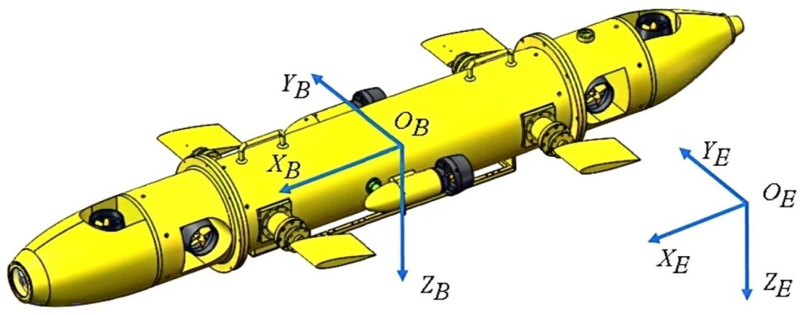
Figure 1. Inertial and body-stationary coordinate frames [15]

3. Problem Formulation

As demonstrated in the literature [11], the motion of the i-th follower AUV is described using 127 both a local stationary coordinate system and a body-stationary coordinate system. Presuming that the 128 multi-AUV system includes N-1 followers and 1 leader. Ignoring roll, pitch, and yaw, the dynamic model of the three-DOF AUV is formulated:

{\dot{β}}_{i} = R_{i} (Φ_{i}) v_{i}

(6)

M_{i} {\dot{v}}_{i} = - D_{i} v_{i} - {\bar{g}}_{i} (Φ_{i}) + τ_{i}

(7)

where

β_{i} = {[\begin{matrix} β_{x_{i}}, β_{y_{i}}, β_{z_{i}} \end{matrix}]}^{T}

represents the local position of the i-th follower, and

{\dot{β}}_{i}

is the temporal derivative of the position, i.e., the velocity.

M_{i}

is the mass matrix of the i-th AUV, and

{\dot{v}}_{i}

is the acceleration of the AUV.

τ_{i} = {[\begin{matrix} τ_{u i}, τ_{v i}, τ_{w i} \end{matrix}]}^{T}

is the external control input torque.

{\bar{g}}_{i} (Φ_{i})

represents the restoring force due to gravity and buoyancy.

D_{i}

represents the damping coefficient matrix, and

v_{i}

is the velocity, reflecting the water resistance’s effect on the AUV’s motion.

R_{i} (Φ_{i})

is a rotation matrix depending on the AUV’s orientation

Φ_{i}

, used to transform the AUV’s velocity

v_{i}

from the body-stationary coordinate system to the local stationary coordinate system. This implies that the actual velocity of the AUV is obtained by transforming its velocity in the body coordinate system through the rotation matrix.

R_{i} (Φ_{i})

represents typically expressed as:

R_{i} (Φ_{i}) = [\begin{matrix} c_{ψ_{i}} c_{θ_{i}} & - s_{ψ_{i}} c_{ϕ_{i}} + s_{ϕ_{i}} s_{θ_{i}} c_{ψ_{i}} & s_{ψ_{i}} s_{ϕ_{i}} + s_{θ_{i}} c_{ϕ_{i}} c_{ψ_{i}} \\ s_{ψ_{i}} c_{θ_{i}} & c_{ψ_{i}} c_{ϕ_{i}} + s_{θ_{i}} s_{ϕ_{i}} s_{ψ_{i}} & - c_{ψ_{i}} s_{ϕ_{i}} + s_{θ_{i}} c_{ϕ_{i}} s_{ψ_{i}} \\ - s_{θ_{i}} & s_{ϕ_{i}} c_{θ_{i}} & c_{ϕ_{i}} c_{θ_{i}} \end{matrix}]

(8)

Assuming that all AUVs are operating in steady state operation, Equation (7) can be reformulated:

\begin{matrix} {\dot{x}}_{i} (t) & = [\begin{matrix} {\dot{β}}_{i} \\ {\dot{v}}_{i} \end{matrix}] = [\begin{matrix} 0 & I \\ 0 & - M_{i}^{- 1} D_{i} \end{matrix}] [\begin{matrix} β_{i} \\ v_{i} \end{matrix}] + [\begin{matrix} 0 \\ M_{i}^{- 1} \end{matrix}] τ_{i} + {Dd}_{i} (t) \\ = A x_{i} (t) + B u_{i} (t) + {Dd}_{i} (t) \end{matrix}

(9)

y_{i} (t) = C x_{i} (t)

(10)

where

A = [\begin{matrix} 0 & I \\ 0 & - M_{i}^{- 1} D_{i} \end{matrix}]

and

B = [\begin{matrix} 0 \\ M_{i}^{- 1} \end{matrix}]

The system is controllable for

[A, B]

and observable for

[A, C]

, with

d_{i} (t)

representing an external perturbation defined as

{\dot{d}}_{i} (t) = S d_{i} (t)

, where S is a fixed real matrix. In a multi-AUV system, the leader is designated as 0 and the follower is labeled from 1 to N. Consider the dynamic equation of the leader as:

{\dot{x}}_{0} (t) = A x_{0} (t) + B u_{0} (t) + D d_{0} (t)

(11)

When

u_{0} (t) = 0

and

d_{0} (t) = 0

, the dynamic equation of the leader simplifies to:

{\dot{x}}_{0} (t) = A x_{0} (t)

(12)

During the movement, the leader remains unaffected by the other followers. To characterize the connection between the leader and the followers, a diagonal matrix is incorporated:

M = diag {a_{10}, a_{20}, \dots, a_{N 0}}

(13)

where

a_{i 0}

represents the linkage weight between the ith follower and the leader. Based on this the Laplace matrix is reconstructed into the following form:

L_{s} = [\begin{matrix} 0 & 0_{1 \times N} \\ - M_{1 N} & L \end{matrix}]

(14)

The first row of the matrix

[0, 0_{1 \times N}]

implies that the leader is not influenced by other followers. The first column of the matrix

[0, - M_{1 N}]

suggests that the followers are influenced by the leader. This configuration also characterizes the connectivity (either cooperation or competition) between the followers through the sub-matrix

L

, the specific structure of which depends on the topology of the connections between the followers. Let

\tilde{L} = D L D

. If Presumption 1 is met, the following lemma also holds:

Lemma 2.

[12]. For a non-singular M-matrix

\tilde{L}

, there exists a positive definite diagonal matrix

Λ = diag {ω_{1}, ω_{2}, \dots, ω_{N}}

such that

Λ {\tilde{L}}_{1} + {\tilde{L}}_{1}^{T} Λ > 0

Lemma 3.

[13]. Given vectors m and n of appropriate dimensions, there is an appropriate positive definite matrix

R > 0

such that

\pm 2 m^{T} n \leq m^{T} R m + n^{T} R^{- 1} n

4. Expanded State Observer Design Scheme

The inverse step method is well-suited for addressing various complex nonlinear systems. By designing appropriate Lyapunov functions and choosing suitable gain matrices, it can be ensured that the observation error dynamics of the system are Hurwitz’s, i.e., meaning the system’s error dynamics exhibit strong robustness. Inspired by [6],we design an extended state observer by backstepping to ensure that the estimates of the states and disturbances approximate their actual values quickly and accurately. The extended state observer, designed by the backstepping, effectively manages complex interactions between different agents and external disturbances, while also simplifying the observer’s construction to achieve good convergence and steadiness, ensuring the observation discrepancy diminishes to zero within a finite period. Define the estimate of the extended state as

{\hat{η}}_{i} (t) = {[\begin{matrix} x_{i}^{T} (t), d_{i}^{T} (t) \end{matrix}]}^{T}

to be

{\hat{η}}_{i}

and define the observation error to be

{\tilde{η}}_{i} = η_{i} - {\hat{η}}_{i}

. The Lyapunov function

V_{1}

is chosen as follows:

V_{1} = \frac{1}{2} {\tilde{η}}_{i}^{T} {\tilde{η}}_{i}

(15)

The derivative of

V_{1}

can be obtained:

{\dot{V}}_{1} = {\tilde{η}}_{i}^{T} {\dot{\tilde{η}}}_{i}

(16)

Substituting into the dynamic equations of the system gives:

{\dot{\tilde{η}}}_{i} = {\dot{η}}_{i} - {\dot{\hat{η}}}_{i} = \bar{A} η_{i} + \bar{B} u_{i} - {\dot{\hat{η}}}_{i}

(17)

The dynamics of the estimates are assumed to be:

{\dot{\hat{η}}}_{i} = \bar{A} {\hat{η}}_{i} + \bar{B} u_{i} + L (y_{i} - {\hat{y}}_{i})

(18)

where L is the observer gain matrix. Consequently, we have:

{\dot{\tilde{η}}}_{i} = \bar{A} {\tilde{η}}_{i} - L C {\tilde{η}}_{i}

(19)

Further can be obtained:

{\dot{V}}_{1} = {\tilde{η}}_{i}^{T} (\bar{A} {\tilde{η}}_{i} - L \bar{C} {\tilde{η}}_{i}) = {\tilde{η}}_{i}^{T} \bar{A} {\tilde{η}}_{i} - {\tilde{η}}_{i}^{T} L \bar{C} {\tilde{η}}_{i}

(20)

In order to ensure that

{\dot{V}}_{1}

remains negative, it is essential in practical engineering applications to choose an appropriate gain matrix L such that

\bar{A} - L \bar{C}

is a Hurwitz matrix, i.e., all eigenvalues possess negative real components. To summarize the above design the extended state observer (ESO) takes the following form:

{\dot{\hat{η}}}_{i} = \bar{A} {\hat{η}}_{i} + \bar{B} u_{i} + L (y_{i} - \bar{C} {\hat{η}}_{i})

(21)

{\hat{y}}_{i} (t) = \bar{C} {\hat{η}}_{i} (t)

(22)

where

L = [\begin{matrix} L_{x} \\ L_{d} \end{matrix}]

is the gain matrix,

\bar{A} = [\begin{matrix} A & D \\ 0 & S \end{matrix}]

\bar{B} = [\begin{matrix} B \\ 0 \end{matrix}]

and

\bar{C} = [\begin{matrix} C & 0 \end{matrix}]

5. Event-Triggered Control Design Scheme

In this segment, we initially define the two-part formation separation regulation goal for the multi-AUV system and design appropriate control inputs, then further analyze the steadiness of the system by constructing the Lyapunov function. Additionally, an activation function is crafted to guarantee the steadiness of the system, and it is demonstrated that no zeno behavior occurs.

5.1. Multi-AUV System Two-Part Formation Separation Control

We definethe formation tracking error during the separation o fa multi-AUV system as:

ε_{i} (t) = x_{i} (t) - σ_{i} x_{0} (t) - h_{i} (t)

(23)

where

x_{i} (t)

represents the state of the ith follower,

x_{0} (t)

denotes the state of the leader, and

σ_{i}

is a constant taking the value of

\pm 1

to indicate cooperation or competition in a two-way queue formation.

h (t) = {[\begin{matrix} h_{1}^{T} (t), h_{2}^{T} (t), \dots, h_{N}^{T} (t) \end{matrix}]}^{T}

is a queueing function that represents the desired position, which is a continuously segmented differentiable function. Thus the regulation goal is defined as:

lim_{t \to \infty} (x_{i} (t) - σ_{i} x_{0} (t) - h_{i} (t)) = 0

(24)

5.2. Design of control inputs and system steadiness

Relying on the extended state observer crafted in the preceding section, we express the regulation input in the following manner:

u_{i} (t) = c K {\hat{ζ}}_{i} (t) - E {\hat{d}}_{i} (t) + H_{i} (t)

(25)

where

c > 0

represents the constant coupling gain and

K \in R^{m \times n}

is the control gain matrix.

H_{i} (t)

is the queuing compensation signal designed as

H_{i} (t) = \tilde{B} ({\dot{h}}_{i} (t) - A h_{i} (t))

, where

\tilde{B} \in R^{q \times n}

is a pseudo-inverse matrix satisfying

\tilde{B} B = I_{n}

. The estimated state

{\hat{ζ}}_{i} (t)

is defined as follows:

{\hat{ξ}}_{i} (t) = \sum_{j \in N_{i}} (| a_{i j} | [({\tilde{x}}_{i} (t) - h_{i} (t)) - sgn (a_{i j}) ({\tilde{x}}_{j} (t) - h_{j} (t))] + | a_{i 0} | ({\tilde{x}}_{i} (t) - h_{i} (t) - σ_{i} x_{0} (t)))

(26)

The estimated state

{\hat{ξ}}_{i} (t)

of each AUV is a synthesis of its relative states, incorporating information about the state error between the ith AUV and its neighboring AUVs. The leader

x_{0} (t)

, with its associated dynamics, contributes to better achieving the global information. The summation term

\sum_{j \in N_{i}}

{\hat{ξ}}_{i} (t)

cumulative effects exerted by all neighboring AUVs of the ith AUV. Neighbor nodes

N_{i}

refer to other intelligences that are directly connected to the ith AUV. This adjacency is depicted by a directed graph where the edge weights

a_{i j}

signify the strength of the connection between the ith AUV and its neighboring AUVs. The state error terms

({\tilde{x}}_{i} (t) - h_{i} (t))

and

({\tilde{x}}_{j} (t) - h_{j} (t))

denote, respectively, the difference between the approximated condition of the ith AUV and its neighboring jth AUV at the moment of triggering

t_{k}^{i}

and its desired queueing position, serving as a measure of the deviation of each AUV relative to its desired position. The symbolic function

sgn (a_{i j})

utilized to describe the nature of the connection weight

a_{i j}

, indicating whether the relationship between AUVs is cooperative or antagonistic. If

a_{i j}

is positive, it indicates a cooperative relationship; if

a_{i j}

is negative, it indicates an antagonistic relationship. This sign function is adjusted in real time to accurately capture the interactions when calculating the state error. The term

| a_{i 0} | ({\tilde{x}}_{i} (t) - h_{i} (t) - σ_{i} x_{0} (t))

indicates the influence of the leader on the ith AUV.

In Equation (26),

{\tilde{x}}_{i} (t) = e^{A (t - t_{k}^{i})} {\hat{x}}_{i} (t_{k}^{i})

is the estimated state of

t_{k}^{i}

at the trigger moment, and its value depends on:

t_{k + 1}^{i} = inf \{t > t_{k}^{i} ∣ f ({\tilde{e}}_{i} (t), {\tilde{ζ}}_{i} (t)) \geq 0\}

(27)

Thus the condition assessment discrepancy can be obtained:

e_{i} (t) = e^{A (t - t_{k}^{i})} {\hat{ζ}}_{i} (t_{k}^{i}) - {\hat{x}}_{i} (t), t \in [t_{k}^{i}, t_{k + 1}^{i})

(28)

Next, we will design the Lyapunov function based on the errors and examine the steadiness of the system accordingly. Consider the following four types of errors:

State estimation error ${\tilde{x}}_{i} (t) = x_{i} (t) - {\hat{x}}_{i} (t)$
Perturbation estimation error ${\tilde{d}}_{i} (t) = d_{i} (t) - {\hat{d}}_{i} (t)$
Queue tracking error $ε_{i} (t) = x_{i} (t) - σ_{i} x_{0} (t) - h_{i} (t)$
Estimate the formation tracking error ${\hat{ε}}_{i} (t) = {\hat{x}}_{i} (t) - σ_{i} x_{0} (t) - h_{i} (t)$

Considering Equation 9 and Equation 21, the dynamic equation for the ESO’s estimation error for the perturbation can be obtained:

{\dot{\tilde{x}}}_{i} (t) = {\dot{x}}_{i} (t) - {\dot{\hat{x}}}_{i} (t) = (A x_{i} (t) + B u_{i} (t) + D d_{i} (t)) - (A {\hat{x}}_{i} (t) + B u_{i} (t) + L (C x_{i} (t) - C {\hat{x}}_{i} (t)))

(29)

Thus it can be obtained:

{\dot{\tilde{x}}}_{i} (t) = A {\bar{x}}_{i} (t) - L C {\bar{x}}_{i} (t) + D {\bar{d}}_{i} (t)

(30)

where

{\bar{x}}_{i} (t) = x_{i} (t) - {\hat{x}}_{i} (t)

and

{\bar{d}}_{i} (t) = d_{i} (t) - {\hat{d}}_{i} (t)

. The derivative of the estimated queue tracking error is:

{\dot{\hat{ε}}}_{i} (t) = {\dot{\hat{x}}}_{i} (t) - σ_{i} {\dot{x}}_{0} (t) - {\dot{h}}_{i} (t)

(31)

Taking into account the dynamic equations of the system one can get:

{\dot{\hat{x}}}_{i} (t) = A {\hat{x}}_{i} (t) + B u_{i} (t) + L (C x_{i} (t) - C {\hat{x}}_{i} (t))

(32)

Combining this with

{\dot{x}}_{0} (t) = A x_{0} (t)

gives:

{\dot{\hat{ε}}}_{i} (t) = A {\hat{x}}_{i} (t) + B u_{i} (t) + L C (x_{i} (t) - {\hat{x}}_{i} (t)) - σ_{i} A x_{0} (t) - {\dot{h}}_{i} (t)

(33)

Substituting

{\hat{ζ}}_{i} (t)

for

u_{i} (t)

yields:

u_{i} (t) = c K (\sum_{j \in N_{i}} (|a_{i j}| ({\hat{ε}}_{i} (t) - sgn (a_{i j}) {\hat{ε}}_{j} (t)) + |a_{i 0}| {\hat{ε}}_{i} (t))) - E {\hat{d}}_{i} (t) + H_{i} (t)

(34)

Bringing in

{\dot{\hat{ε}}}_{i} (t)

gives further:

\begin{matrix} {\dot{\hat{ε}}}_{i} (t) = & A {\hat{x}}_{i} (t) + c B K (\sum_{j \in N_{i}} (|a_{i j}| ({\hat{ε}}_{i} (t) - sgn (a_{i j}) {\hat{ε}}_{j} (t))) + |a_{i 0}| {\hat{ε}}_{i} (t)) \\ + L C {\bar{x}}_{i} (t) - σ_{i} A x_{0} (t) - {\dot{h}}_{i} (t) \end{matrix}

(35)

Combined with the error phase Equation 28, this gives:

\begin{matrix} {\hat{ε}}_{i} (t) = & c B K (\sum_{j \in N_{i}} [|a_{i j}| ({\hat{ε}}_{i} (t) - sgn (a_{i j}) {\hat{ε}}_{j} (t)) + |a_{i 0}| {\hat{ε}}_{i} (t)] \\ + \sum_{j \in N_{i}} [|a_{i j}| (e_{i} (t) - sgn (a_{i j}) e_{j} (t)) + |a_{i 0}| e_{i} (t)]) + A {\hat{ε}}_{i} (t) + L C {\bar{x}}_{i} (t) \end{matrix}

(36)

In order to more intuitively understand the components of the estimated state

{\hat{ζ}}_{i} (t)

, we re-express Equation 26 as follows:

{\hat{ξ}}_{i} (t) = \sum_{j \in N_{i}} (|a_{i j}| ({\hat{ε}}_{i} (t) - sgn (a_{i j}) {\hat{ε}}_{j} (t)) + |a_{i 0}| {\hat{ε}}_{i} (t)) + \sum_{j \in N_{i}} (|a_{i j}| (e_{i} (t) - sgn (a_{i j}) e_{j} (t)) + |a_{i 0}| e_{i} (t))

(37)

Decompose the estimated state

{\hat{ζ}}_{i} (t)

into two parts: queue tracking error and state measurement error. The first part is the effect of the formation tracking error:

\sum_{j \in N_{i}} (|a_{i j}| ({\hat{ε}}_{i} (t) - sgn (a_{i j}) {\hat{ε}}_{j} (t)) + |a_{i 0}| {\hat{ε}}_{i} (t))

(38)

This part represents the relationship between the formation tracking error of each ith AUVand its neighboring jth AUV, as well as the formation tracking error between the ith AUV and the leader. It clearly illustrates how the individual intelligences interact with each other during the formation control process, especially when considering cooperative and adversarial relationships.

The second part addresses the effect of state measurement error:

\sum_{j \in N_{i}} (| a_{i j} | (e_{i} (t) - sgn (a_{i j}) e_{j} (t)) + | a_{i 0} | e_{i} (t))

(39)

This partly represents the relationship between the state measurement errors of the ith AUV and its neighboring jth AUV, as well as the state measurement errors between the ith AUV and the leader. In order to simplify the expression form and conduct a more systematic analysis of the overall multi-AUV system, the responsive conduct of the system can be accurately depicted using a matrix formulation:

Estimated state vector $\hat{ζ} (t)$ :

$\hat{ζ} (t) = {[{\hat{ζ}}_{1}^{T} (t), {\hat{ζ}}_{2}^{T} (t), \dots, {\hat{ζ}}_{N}^{T} (t)]}^{T}$

(40)
State measurement error vector $e (t)$ :

$e (t) = {[e_{1}^{T} (t), e_{2}^{T} (t), \dots, e_{N}^{T} (t)]}^{T}$

(41)
Estimate the queue tracking error vector $\hat{ε} (t)$ :

$\hat{ε} (t) = {[{\hat{ε}}_{1}^{T} (t), {\hat{ε}}_{2}^{T} (t), \dots, {\hat{ε}}_{N}^{T} (t)]}^{T}$

(42)
State estimation error vector $\bar{x} (t)$ :

\bar{x} (t) = {[{\bar{x}}_{1}^{T} (t), {\bar{x}}_{2}^{T} (t), \dots, {\bar{x}}_{N}^{T} (t)]}^{T}

(43)

The following equation from graph theory is also introduced to handle the presence of both positive and negative weights in signed graphs, thereby simplifies the related computations:

\begin{matrix} σ_{i} σ_{j} a_{i j} = |a_{i j}| \\ |a_{i 0}| sgn (a_{i 0}) = a_{i 0} \\ a_{i j} σ_{j} = a_{i j} σ_{i} sgn (a_{i j}) \end{matrix}

(44)

Equations 26 and 36 can then be compressed into matrix form. Equation 26 is compressed as:

\hat{ξ} (t) = (L \otimes I_{n}) (\hat{ε} (t) + e (t))

(45)

Here

L

is the Laplace matrix,

I_{n}

is an n-dimensional unit matrix, and ⊗ denotes the Kronecker product. Equation 36 is expressed in compressed form as:

\dot{\hat{ε}} (t) = (I_{N} \otimes A + c L \otimes B K) \hat{ε} (t) + (c L \otimes B K) e (t) + (I_{N} \otimes F_{1} C) \bar{x} (t)

(46)

Remark 1.

The Kronecker product is a potent and efficient instrument for depicting the dynamic behavior of of a multi-AUV system. It allows for a concise description of the states and control inputs of all underwater robots in the system by extending the matrices to a higher dimensional space. For example,

L \otimes I_{n}

denotes the extension of the Laplace matrix

L

to an N-dimensional space, enabling the representation of the interrelationships among all underwater robots. This approach not only simplifies the numerical depiction, but also effectively captures the dynamic interactions between individual underwater robots. The analysis of the overall system can be simplified by integrating the state errors and tracking errors of all underwater robots into the vectors

\hat{ζ} (t)

and

e (t)

. This method of integrating state errors enhances computational efficiency and provides a more intuitive reflection of the system’s overall responsive conduct, aiding in the design of globally coordinated control strategies. This approach is particularly effective when dealing with complex multi-AUV systems, as it facilitates a better understanding of the global dynamics and improves the robustness of the control algorithm. The Laplace matrix L serves a significant function in describing the topology of a graph and is crucial in the analysis of multiple underwater robotic systems. The eigenvalues and eigenvectors of the Laplace matrix can be used to assess the steadiness and consistency of the system. In addition, the zero eigenvalues of the Laplace matrix correspond to the global coherent state of the system, while the non-zero eigenvalues provide critical insights into the dynamic behavior of the system.

A further attempt to normalize the above formula is to convert it, defining the canonical form as:

\tilde{e} (t) = (D \otimes I_{n}) e (t)

(47)

\tilde{ε} (t) = (D \otimes I_{n}) \hat{ε} (t)

(48)

Substituting

\hat{ζ} (t)

and

\ddot{\hat{ζ}} (t)

into the original

\dot{\hat{ζ}} (t)

and

\dot{e} (t)

dynamic equations, we have the derivatives after computing the canonical transformations as:

\dot{\tilde{ε}} (t) = (D \otimes I_{n}) \dot{\hat{ε}} (t)

(49)

\ddot{\hat{ζ}} (t) = (D \otimes I_{n}) \dot{e} (t)

(50)

Then replace

\hat{ϵ} (t)

and

e (t)

with

\tilde{ϵ} (t)

and

\tilde{e} (t)

in the original equation:

\hat{ε} (t) = (D^{- 1} \otimes I_{n}) \tilde{ε} (t)

(51)

e (t) = (D^{- 1} \otimes I_{n}) \tilde{e} (t)

(52)

Thus:

\begin{matrix} \dot{\tilde{ε}} (t) = & (D \otimes I_{n}) [(I_{N} \otimes A + c L \otimes B K) (D^{- 1} \otimes I_{n}) \tilde{ε} (t) \\ + (c L \otimes B K) (D^{- 1} \otimes I_{n}) \tilde{e} (t) + (I_{N} \otimes L C) \bar{x} (t)] \end{matrix}

(53)

\begin{matrix} \dot{\tilde{e}} (t) = & (D \otimes I_{n}) [(I_{N} \otimes A - c L \otimes B K) (D^{- 1} \otimes I_{n}) \tilde{e} (t) \\ - (c L \otimes B K) (D^{- 1} \otimes I_{n}) \tilde{ε} (t) - (I_{N} \otimes B) H (t) - (I_{N} \otimes L C) \bar{x} (t)] \end{matrix}

(54)

Using

D D^{- 1} = I_{N}

, the simplification yields:

\dot{\tilde{ε}} (t) = (I_{N} \otimes A + c \tilde{L} \otimes B K) \tilde{ε} (t) + (c \tilde{L} \otimes B K) \tilde{e} (t) + (D \otimes L C) \bar{x} (t)

(55)

\dot{\tilde{e}} (t) = (I_{N} \otimes A - c \tilde{L} \otimes B K) \tilde{e} (t) + (c \tilde{L} \otimes B K) \tilde{ε} (t) + (D \otimes B) H (t) + (D \otimes L C) \bar{x} (t)

(56)

Based on our design of the extended state observer in the previous section, the dynamic equation for the extended state estimation error is:

{\dot{\bar{η}}}_{i} (t) = (\bar{A} - L \bar{C}) {\bar{η}}_{i} (t)

(57)

If the matrix L is crafted in such a way that

\bar{A} - L \bar{C}

is a Hurwitz matrix, then

{\bar{η}}_{i} (t)

will converge asymptotically to zero. Consequently,

\bar{x} (t)

and

{\bar{d}}_{i} (t)

will also gradually diminish to zero.We perform an equivalent decomposition of the dynamic equations of the AUV system, and since

\bar{x} (t)

is able to converge asymptotically to zero, this effect can be neglected when analyzing steadiness. Therefore, Equation 55 can be simplified as:

\dot{\tilde{ε}} (t) = (I_{N} \otimes A + c \tilde{L} \otimes B K) \tilde{ε} (t) + (c \tilde{L} \otimes B K) \tilde{e} (t)

(58)

Similarly, for Equation 56 one gets, we have:

\dot{\tilde{e}} (t) = (I_{N} \otimes A - c \tilde{L} \otimes B K) \tilde{e} (t) + (c \tilde{L} \otimes B K) \tilde{ε} (t) + (D \otimes B) H (t) + (D \otimes L C) \bar{x} (t)

(59)

Since

\bar{x} (t)

is asymptotically convergent to zero, the effect of this term can be ignored when analyzing steadiness. Thus, Equation 56 simplifies to:

\dot{\tilde{e}} (t) = (I_{N} \otimes A - c \tilde{L} \otimes B K) \tilde{e} (t) + (c \tilde{L} \otimes B K) \tilde{ε} (t) + (D \otimes B) H (t)

(60)

In summary, a candidate Lyapunov function

V (t)

is chosen to examine the steadiness of the entire system:

V (t) = {\tilde{ε}}^{T} (t) (Λ \otimes P) \tilde{ε} (t)

(21)

where

Λ

is a diagonal matrix and P is a symmetric positive definite matrix. This configuration of the Lyapunov function is crafted to efficiently measure the magnitude of the error vector

\tilde{ε} (t)

. Next, the temporal derivative of the Lyapunov function

V (t)

along the path of the system is computed as follows:

\dot{V} (t) = \frac{d}{d t} ({\tilde{ε}}^{T} (t) (Λ \otimes P) \tilde{ε} (t))

(61)

Use the chain rule for derivatives to get:

\dot{V} (t) = 2 {\tilde{ε}}^{T} (t) (Λ \otimes P) \dot{\tilde{ε}} (t)

(62)

Substituting

\dot{\tilde{ε}} (t)

, the temporal derivative of the Lyapunov function becomes:

\dot{V} (t) = 2 {\tilde{ε}}^{T} (t) (Λ \otimes P) [(I_{N} \otimes A + c \tilde{L} \otimes B K) \tilde{ε} (t) + (c \tilde{L} \otimes B K) \tilde{e} (t)]

(63)

Expand and simplify the above equation:

\begin{matrix} \dot{V} (t) & = 2 {\tilde{ε}}^{T} (t) (Λ \otimes P) (I_{N} \otimes A) \tilde{ε} (t) + 2 {\tilde{ε}}^{T} (t) (Λ \otimes P) (c \tilde{L} \otimes B K) \tilde{ε} (t) \\ + 2 {\tilde{ε}}^{T} (t) (Λ \otimes P) (c \tilde{L} \otimes B K) \tilde{e} (t) \end{matrix}

(64)

Using the properties of the Kronecker product, this is further simplified to:

\begin{matrix} \dot{V} (t) & = {\tilde{ε}}^{T} (t) [Λ \otimes (P A + A^{T} P)] \tilde{ε} (t) + c {\tilde{ε}}^{T} (t) [(Λ \tilde{L} + {\tilde{L}}^{T} Λ) \otimes P B K + K^{T} B^{T} P] \tilde{ε} (t) \\ + 2 c {\tilde{ε}}^{T} (t) [(Λ \tilde{L}) \otimes P B K] \tilde{e} (t) \end{matrix}

(65)

Construct the positive definite matrix according to Lemma 2:

\hat{L} = Λ \tilde{L} + {\tilde{L}}^{T} Λ

(66)

The steadiness of the system can be ensured by introducing a positive definite matrix.To further analyze the system steadiness conditions, the upper bound is further estimated using Lemma 3:

\begin{matrix} \dot{V} (t) & \leq {\tilde{ε}}^{T} (t) [Λ \otimes (P A + A^{T} P - \frac{c λ_{min} (\hat{L})}{2 λ_{max} (Λ)} P B B^{T} P)] \tilde{ε} (t) \\ + \frac{2 c λ_{max} (Λ)}{λ_{min} (\hat{L})} {\tilde{e}}^{T} (t) ({\tilde{L}}^{T} Λ \tilde{L} \otimes P B B^{T} P) \tilde{e} (t) \end{matrix}

(67)

The right half of the above equation is the perturbation part. To simplify the computation, we define the existence of

M_{1}

M_{1} = Λ \hat{L} + L^{T} Λ

(68)

Thus

\dot{V} (t)

can be expressed as:

\dot{V} (t) = {\tilde{ε}}^{T} (t) (Λ \otimes (P A + A^{T} P)) \tilde{ε} (t) + 2 c {\tilde{ε}}^{T} (t) (M_{1} \otimes P B K) \tilde{ε} (t) + 2 c {\tilde{ε}}^{T} (t) (M_{1} \otimes P B K) \tilde{e} (t)

(69)

By Lyapunov’s theorem, we want

\dot{V} (t)

to be negative and need to introduce

m_{1}

and

m_{2}

to control the above sub-terms. To this end, we construct

M_{1}

satisfying:

M_{1} = m_{1} I

(70)

This allows us to express

\dot{V} (t)

as:

\dot{V} (t) = {\tilde{ε}}^{T} (t) (Λ \otimes (P A + A^{T} P + 2 c m_{1} P B K)) \tilde{ε} (t) + 2 c {\tilde{ε}}^{T} (t) (m_{1} I \otimes P B K) \tilde{e} (t)

(71)

Next,

m_{2}

is introduced to further decompose the error term:

m_{2} = \frac{2 c λ_{max} (Λ) ∥{\tilde{L}}^{T} Λ \tilde{L} \otimes P B K∥}{δ λ_{min} (Λ) λ_{min} (\tilde{L})}

(72)

Substitution gives:

\dot{V} (t) \leq \sum_{i = 1}^{N} δ λ_{min} (Λ) [(m_{1} - 1) ∥ {\bar{ε}}_{i} (t) ∥^{2} + (\frac{1}{m_{1}} + m_{2} - 1) {∥ {\tilde{e}}_{i} (t) ∥}^{2}]

(73)

5.3. Design of Trigger Functions and Proof of No Zeno Behavior

In event-triggered control, trigger functions are introduced to ascertain the optimal timing for updating the regulation input. This approach reduces the frequency of computation and communication and ensures the steadiness of the system. From the perspective of steadiness conditions, incorporating a trigger function into the construction of the Lyapunov function allows for a more precise estimation of the error term, thereby facilitating the proof of the system’s asymptotic steadiness. We choose to construct a proportional trigger function, defined in:

f ({\tilde{e}}_{i} (t), {\tilde{ζ}}_{i} (t)) = ∥ {\tilde{e}}_{i} {(t) ∥}^{2} - c_{1} ∥ {\tilde{ζ}}_{i} {(t) ∥}^{2} - c_{2} {∥ {\tilde{ζ}}_{i} (t) ∥}^{4}

(74)

When the trigger condition is satisfied, i.e:

∥ {\tilde{e}}_{i} {(t) ∥}^{2} < c_{1} ∥ {\tilde{ζ}}_{i} {(t) ∥}^{2} + c_{2} {∥ {\tilde{ζ}}_{i} (t) ∥}^{4}

(75)

Since

\tilde{ξ} (t) = (\tilde{L} \otimes I_{n}) (\tilde{ε} (t) + \tilde{e} (t))

, one can go on to deduce that we get:

∥ \tilde{ξ} {(t) ∥}^{2} \leq ∥ \tilde{L} ∥^{2} {∥ \tilde{ε} (t) + \tilde{e} (t) ∥}^{2}

(76)

Combined with the designed trigger condition in Equation 5, it can be further obtained:

| {\tilde{e}}_{i} {(t) ∥}^{2} < c_{1} | \tilde{L} ∥^{2} | \tilde{ε} (t) + \tilde{e} {(t) ∥}^{2} + c_{2} | \tilde{L} ∥^{4} {| \tilde{ε} (t) + \tilde{e} (t) ∥}^{4}

(77)

To further estimate the temporal derivative of the Lyapunov function, the above upper bound estimate is brought to the Lyapunov function:

\begin{matrix} \dot{V} (t) & \leq \sum_{i = 1}^{N} δ λ_{min} (Λ) [(m_{1} - 1) ∥ {\bar{ε}}_{i} (t) ∥^{2} + (\frac{1}{m_{1}} + m_{2} - 1) {∥ {\tilde{e}}_{i} (t) ∥}^{2}] \\ \leq \sum_{i = 1}^{N} δ λ_{min} (Λ) [(m_{1} - 1) {∥ {\bar{ε}}_{i} (t) ∥}^{2} \\ + (\frac{1}{m_{1}} + m_{2} - 1) (c_{1} ∥ \tilde{L} ∥^{2} {∥ \tilde{ε} (t) + \tilde{e} (t) ∥}^{2} \\ + c_{2} ∥ \tilde{L} ∥^{4} ∥ \tilde{ε} (t) + \tilde{e} (t) ∥^{4})] \end{matrix}

(78)

From the above derivation, it can be seen that when the appropriate parameters

c_{1}

and

c_{2}

are chosen, it can be ensured that

\dot{V} (t) < 0

. i.e., it is satisfied:

(m_{1} - 1) + (\frac{1}{m_{1}} + m_{2} - 1) c_{1} k < 0

(79)

(\frac{1}{m_{1}} + m_{2} - 1) c_{2} k^{2} < 0

(80)

It can be seen that we need to solve for both inequalities to arrive at

c_{1}

and

c_{2}

. For Equation 58, the solution of

c_{1}

is obtained by shifting terms and transformations:

c_{1} > \frac{1 - m_{1}}{k (\frac{1}{m_{1}} + m_{2} - 1)}

(81)

Similarly, for Equation 59 it is straightforward to solve the expression for

c_{2}

as:

c_{2} < 0

(82)

To ensure that

\dot{V} (t) < 0

, it is necessary to choose

c_{1}

and

c_{2}

that satisfy the above constraints, so we choose:

c_{1} = \frac{2 (1 - m_{1})}{k (\frac{1}{m_{1}} + m_{2} - 1)}

(83)

c_{2} = - \frac{1}{k^{2} (\frac{1}{m_{1}} + m_{2} - 1)}

(84)

The above

c_{1}

and

c_{2}

not only satisfy the constraints, but also ensure that the temporal derivative of the Lyapunov function is negative, which in turn ensures the asymptotic steadiness of the system. Summarizing the above, the new trigger function and its parameters are expressed as follows:

f ({\tilde{e}}_{i} (t), {\tilde{ξ}}_{i} (t)) = ∥ {\tilde{e}}_{i} {(t) ∥}^{2} - (\frac{2 (1 - m_{1})}{k (\frac{1}{m_{1}} + m_{2} - 1)}) ∥ {\tilde{ξ}}_{i} {(t) ∥}^{2} - (- \frac{1}{k^{2} (\frac{1}{m_{1}} + m_{2} - 1)}) {∥ {\tilde{ξ}}_{i} (t) ∥}^{4}

(85)

where,

m_{1} \in (0, 1)

\begin{matrix} m_{1} \in (0, 1) \\ m_{2} = \frac{2 c λ_{max} (Λ) ∥{\tilde{L}}^{T} Λ \tilde{L} \otimes P B B^{T} P∥}{δ λ_{min} (Λ) λ_{min} (\tilde{L})} \\ c \geq \frac{2 λ_{max} (Λ)}{λ_{min} (L)} \\ k = ∥ \tilde{L} ∥^{2} \end{matrix}

(86)

c \geq \frac{2 λ_{max} (Λ)}{λ_{min} (L)}

k = ∥ \hat{L} ∥^{2}

Next we analyze whether the system is free of zeno behavior under this trigger function. The system’s estimation error dynamics equations Equation 58 and Equation 59 define the parameter

φ (t) = \frac{∥ \tilde{e} (t) ∥}{∥ \tilde{ζ} (t) ∥}

and compute its derivatives:

\frac{d}{d t} (\frac{∥ \tilde{e} (t) ∥}{∥ \tilde{ζ} (t) ∥}) \leq \frac{∥ \dot{\tilde{e}} (t) ∥}{∥ \tilde{ζ} (t) ∥} + \frac{∥ \tilde{e} (t) ∥ ∥ \dot{\tilde{ζ}} (t) ∥}{∥ \tilde{ζ} {(t) ∥}^{2}}

(87)

By analyzing the dynamic equation of the estimation error, it can be obtained:

\dot{φ} (t) \leq (1 + φ (t)) (α + β φ (t))

(88)

where

α

and

β

are system parameters, specifically:

α_{1} = \frac{∥ c \tilde{L} \otimes B K ∥ ∥ \tilde{ε} (t) ∥ + ∥ D \otimes L C ∥ ∥ \bar{x} (t) ∥ + θ}{∥ \tilde{ξ} (t) ∥}

(89)

α_{2} = \frac{∥ \tilde{L} \otimes I_{N} ∥ ∥ I_{N} \otimes A + 2 c \tilde{L} \otimes B K ∥ ∥ \tilde{ε} (t) ∥ + 2 ∥ D \otimes L C ∥ ∥ \bar{x} (t) ∥ + θ ∥ \tilde{ξ} (t) ∥}{∥ \tilde{ζ} (t) ∥}

(90)

where

θ = ∥ I_{N} \otimes B D ∥ κ, κ = {sup}_{i = 1}^{N} ∥ H_{i} (t) ∥

Therefore,

α = max (α_{1}, α_{2})

(92)

Arguments

β_{1}

and

β_{2}

are designed as:

β_{1} = ∥ I_{N} \otimes A - c \tilde{L} \otimes B K ∥

(93)

β_{2} = ∥ \tilde{L} \otimes I_{N} ∥ ∥ I_{N} \otimes A ∥

(94)

Therefore

β = max (β_{1}, β_{2})

(95)

When

φ (t)

grows most rapidly, the initial solution takes the form:

φ (t) = \frac{α e^{(α - β) (t + μ)} - 1}{1 - β e^{(α - β) (t + μ)}}

(96)

where

μ = \frac{1}{β - α} ln α

Ensure that the system does not exhibit zeno behavior by designing trigger conditions and calculating the event interval time

τ

. In order to calculate the minimum event interval time

τ

, the following conditions need to be met:

ζ \sqrt{N} \frac{α e^{(α - β) (τ + μ)} - 1}{1 - β e^{(α - β) (τ + μ)}} = {(\frac{2 (1 - m_{1})}{k (\frac{1}{m_{1}} + m_{2} - 1)})}^{1 / 2}

(97)

Solving the above equation yields a lower bound on the event interval:

τ = \frac{1}{α - β} ln \frac{α (χ + 1)}{α + β χ} > 0

(98)

where

χ = ζ \sqrt{N} {(\frac{2 (1 - m_{1})}{k (\frac{1}{m_{1}} + m_{2} - 1)})}^{1 / 2}

This is a strictly positive time interval, illustrating that the system does not display zeno behavior under trigger regulation.

6. Simulation Results

The effectiveness of the designed control scheme for the AUV formation separation task is next demonstrated through numerical simulations. The scenario involves a multi-AUV system comprising 1 leader and 8 followers, as illustrated in Figure 2(a). The objective is to separate this system into two approximately stable formations, as depicted in Figure 2(b), i.e., into

V_{1} = {1, 2, 3, 4}

and

V_{2} = {5, 6, 7, 8}

with the designed event-triggered control strategy. The collaborative and adversarial conduct among different followers are depicted by black and yellow lines. Each AUV is assigned identical kinetic parameters as specified in [6]. A disturbance gain is then constructed to simulate external perturbations matrix for external positional disturbances

D = [\begin{matrix} 0.5 & - 1 \\ 0.5 & - 1 \\ 1 & 0.5 \\ 0.5 & - 1 \\ 0.5 & - 1 \\ 1 & 0.5 \end{matrix}]

S = [\begin{matrix} 0 & - 1.5 \\ 1.3 & 0 \end{matrix}]

Control Gain Matrix

K = [\begin{matrix} - 1.6657 & 0 & 0 \\ - 7.4026 & 0 & 0 \\ 0 & - 1.3550 & 0.0159 \\ 0 & - 7.9752 & 0.0051 \\ 0 & - 0.0056 & - 1.7425 \\ 0 & 0.0051 & - 11.5208 \end{matrix}]

For the event-triggering mechanism, we calculate the parameters as follows:

c = 6.785

m_{1} = 0.5

m_{2} = 1.5189

, and

k = 14.9391

. The specific trajectory of the formation separation process is depicted in Figure 3. Additionally, as illustrated in Figure 5, the leader leads the two groups of followers into forming two stable rectangular formations. Figure 4 demonstrates the frequency of control input triggers for each AUV during the simulation, demonstrating that the trigger function effectively prevents Zeno behavior. Figure 6 demonstrates the estimation error for the unknown perturbation, clearly showing that the error converges to 0 after 50 seconds of simulation, thus verifying the effectiveness of the extended state monitor. Figure 7 illustrates the convergence of the velocity error for a single AUV during operation, while Figure 8 shows the convergence of the position error for a single AUV during operation, indicating enhanced performance of each AUV during operation.

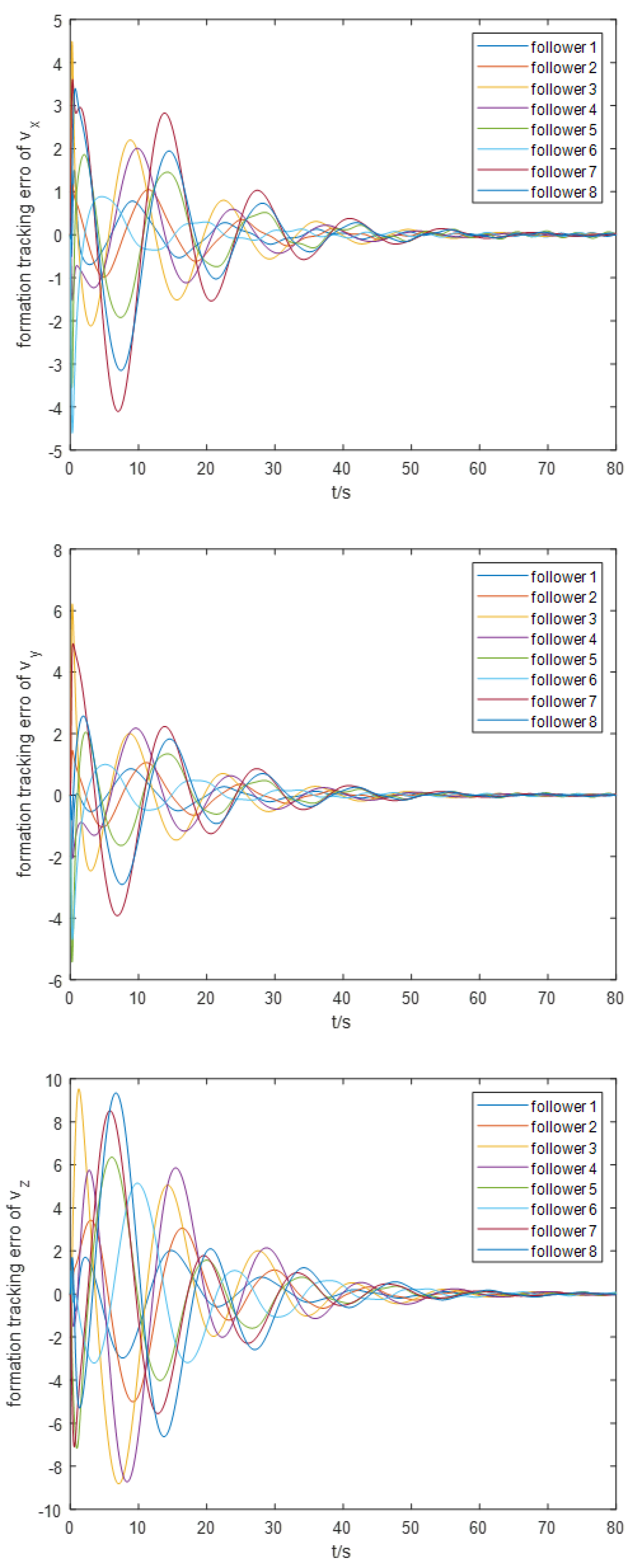
Next, we proceed to examine the steadiness of the overall AUV formation. The formation position tracking error and formation speed tracking error are illustrated in Figure 9 and Figure 10, respectively. It is evident that these two parameters exhibit significant oscillations and slow convergence at the initial stages of the simulation, but ultimately converge within a small neighborhood near the origin, achieving asymptotic steadiness. This behavior can be attributed to the insufficient clarity of the formation tracking regulation goals in the previous section. We intend to conduct a more detailed study on the constraints related to these regulation goals in future research.

7. Conclusion

In this paper,we present an investigation into an event-triggered control scheme incorporating an extended state observer, aimed at achieving formation separation in a multi-AUV system subject to both external interference and internal competition.The proposed event-triggered control scheme is free from zeno behavior and significantly reduce the communication cost. In addition, numerical simulations demonstrate the system’s steadiness under this control scheme, with rapid error can converge observed.In future study,we explore strategies to enhance the convergence performance of formation tracking errors in AUV systems.

References

Yan, Z.; Zhang, C.; Tian, W.; et al. Distributed observer-based formation trajectory tracking method of leader-following multi-AUV system. Ocean Engineering 2022, 260, 112019. [Google Scholar] [CrossRef]
Li, J.; Tian, Z.; Zhang, H. Discrete-time AUV formation control with leader-following consensus under time-varying delays. Ocean Engineering 2023, 286, 115678. [Google Scholar] [CrossRef]
Cai, L.; Sun, Q. Multiautonomous underwater vehicle consistent collaborative hunting method based on generative adversarial network. International Journal of Advanced Robotic Systems 2020, 17. [Google Scholar] [CrossRef]
Altafini, C. Consensus problems on networks with antagonistic interactions. IEEE Transactions on Automatic Control 2012, 58, 935–946. [Google Scholar] [CrossRef]
Liu, G.; Basin, M.V.; Liang, H.; et al. Adaptive bipartite tracking control of nonlinear multiagent systems with input quantization. IEEE Transactions on Cybernetics 2020, 52, 1891–1901. [Google Scholar] [CrossRef] [PubMed]
Xu, Y.; Li, T.; Tong, S. Event-triggered adaptive fuzzy bipartite consensus control of multiple autonomous underwater vehicles. IET Control Theory & Applications 2020, 14, 3632–3642. [Google Scholar]
Zhang, H.; Feng, G.; Yan, H.; et al. Observer-based output feedback event-triggered control for consensus of multi-agent systems. IEEE Transactions on Industrial Electronics 2013, 61, 4885–4894. [Google Scholar] [CrossRef]
Cao, L.; Pan, Y.; Liang, H.; et al. Observer-based dynamic event-triggered control for multiagent systems with time-varying delay. IEEE Transactions on Cybernetics 2022, 53, 3376–3387. [Google Scholar] [CrossRef] [PubMed]
Su, B.; Wang, H.; Wang, Y. Dynamic event-triggered formation control for AUVs with fixed-time integral sliding mode disturbance observer. Ocean Engineering 2021, 240, 109893. [Google Scholar] [CrossRef]
Altafini, C. Consensus problems on networks with antagonistic interactions. IEEE Transactions on Automatic Control 2012, 58, 935–946. [Google Scholar] [CrossRef]
Zhao, L.; Yu, J.Y.; Hu, H. Distributed Adaptive Consensus Tracking Control for Multiple AUVs. In Proceedings of the Seventh International Conference on Information Science and Technology (ICIST), Da Nang, Vietnam, 16-19 April 2017; pp. 480–484. [Google Scholar]
Zhang, H.; Li, Z.; Qu, Z.; et al. On constructing Lyapunov functions for multi-agent systems. Automatica 2015, 58, 39–42. [Google Scholar] [CrossRef]
Wang, C.; Zuo, Z.; Gong, Q.; et al. Formation control with disturbance rejection for a class of Lipschitz nonlinear systems. Science China Information Sciences 2017, 60, 1–11. [Google Scholar] [CrossRef]
Ge, M.F.; Gu, Z.W.; Su, P.; et al. State-constrained bipartite tracking of interconnected robotic systems via hierarchical prescribed-performance control. Nonlinear Dynamics 2023, 111, 9275–9288. [Google Scholar] [CrossRef]
Kang, S.; Rong, Y.; Chou, W. Antidisturbance control for AUV trajectory tracking based on fuzzy adaptive extended state observer. Sensors 2020, 20, 7084. [Google Scholar] [CrossRef] [PubMed]

Figure 2. Communication topology of multi-AUV systems under directed graphs

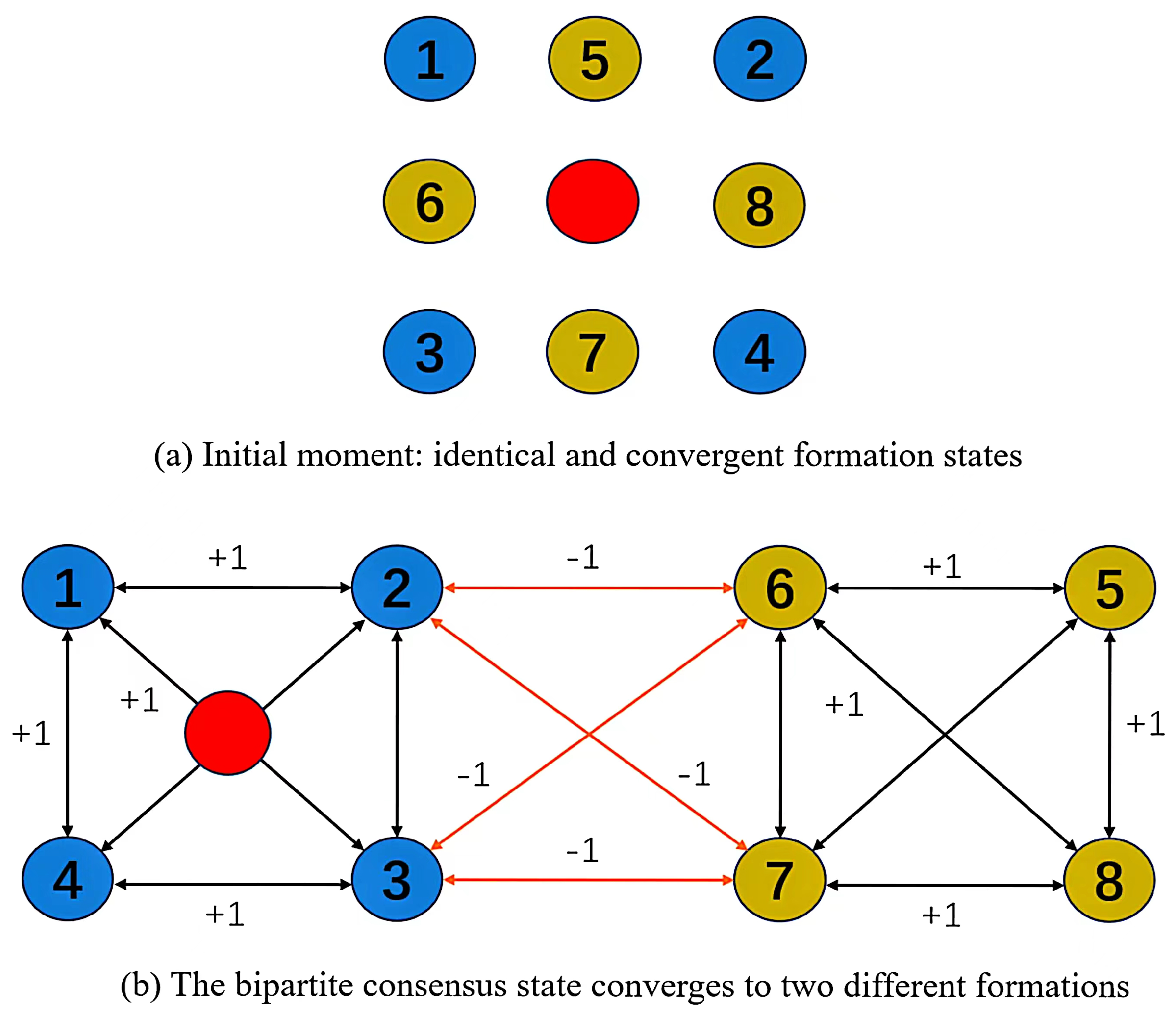
Figure 3. Detailed trajectories during formation separation of multi-AUV systems

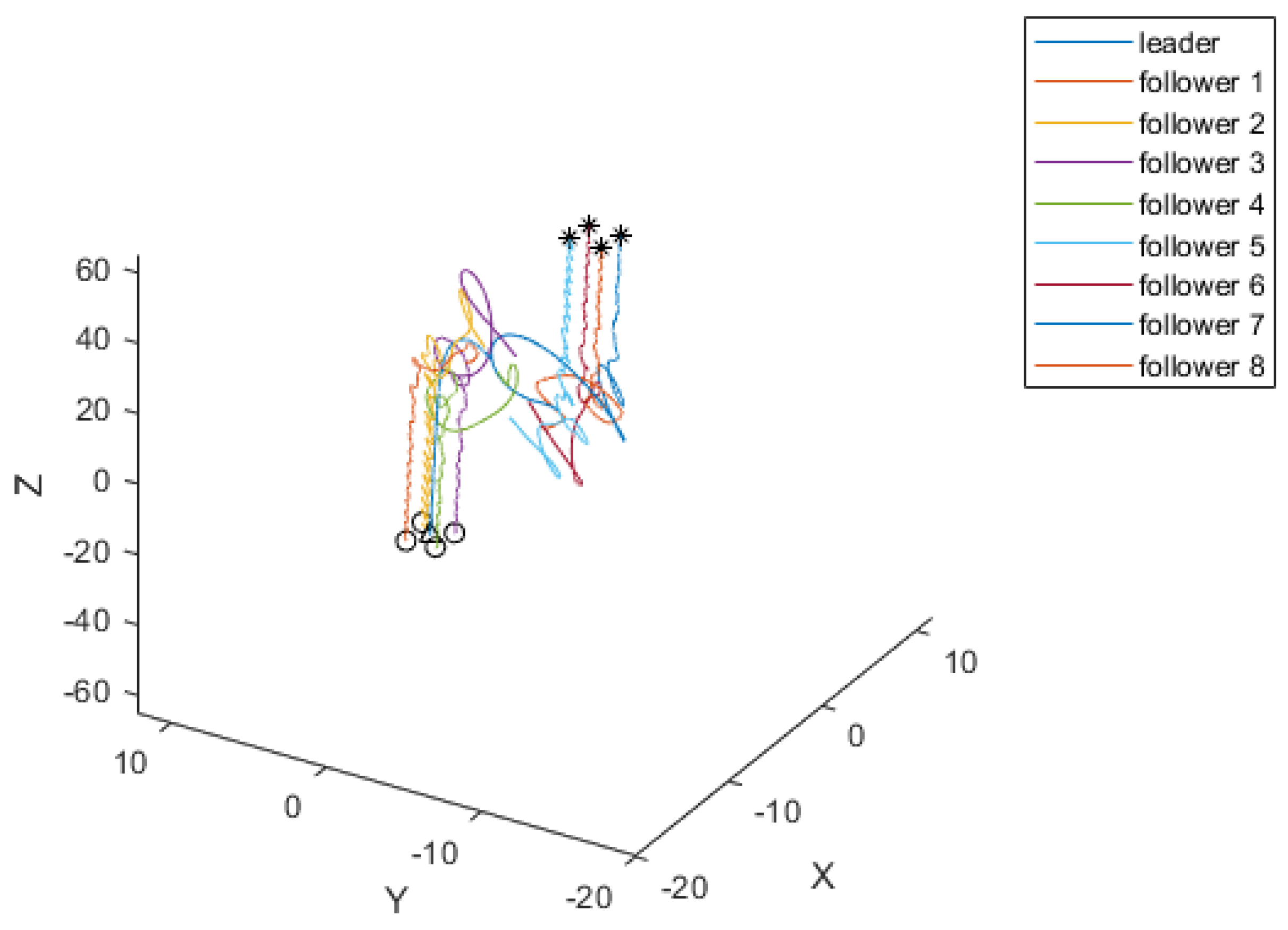
Figure 4. Control input trigger frequency per AUV

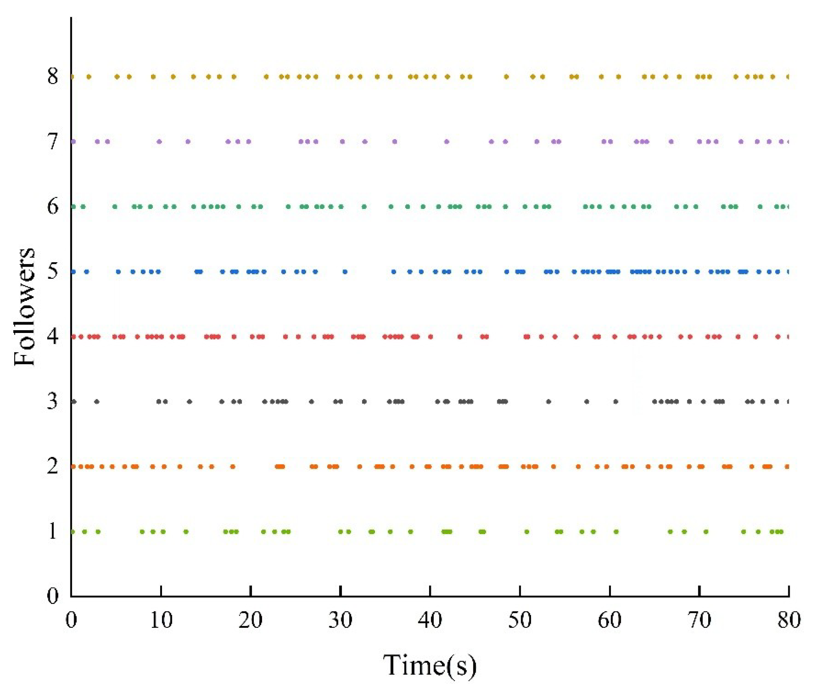
Figure 5. The leader leads two groups of followers in two stable rectangular formations

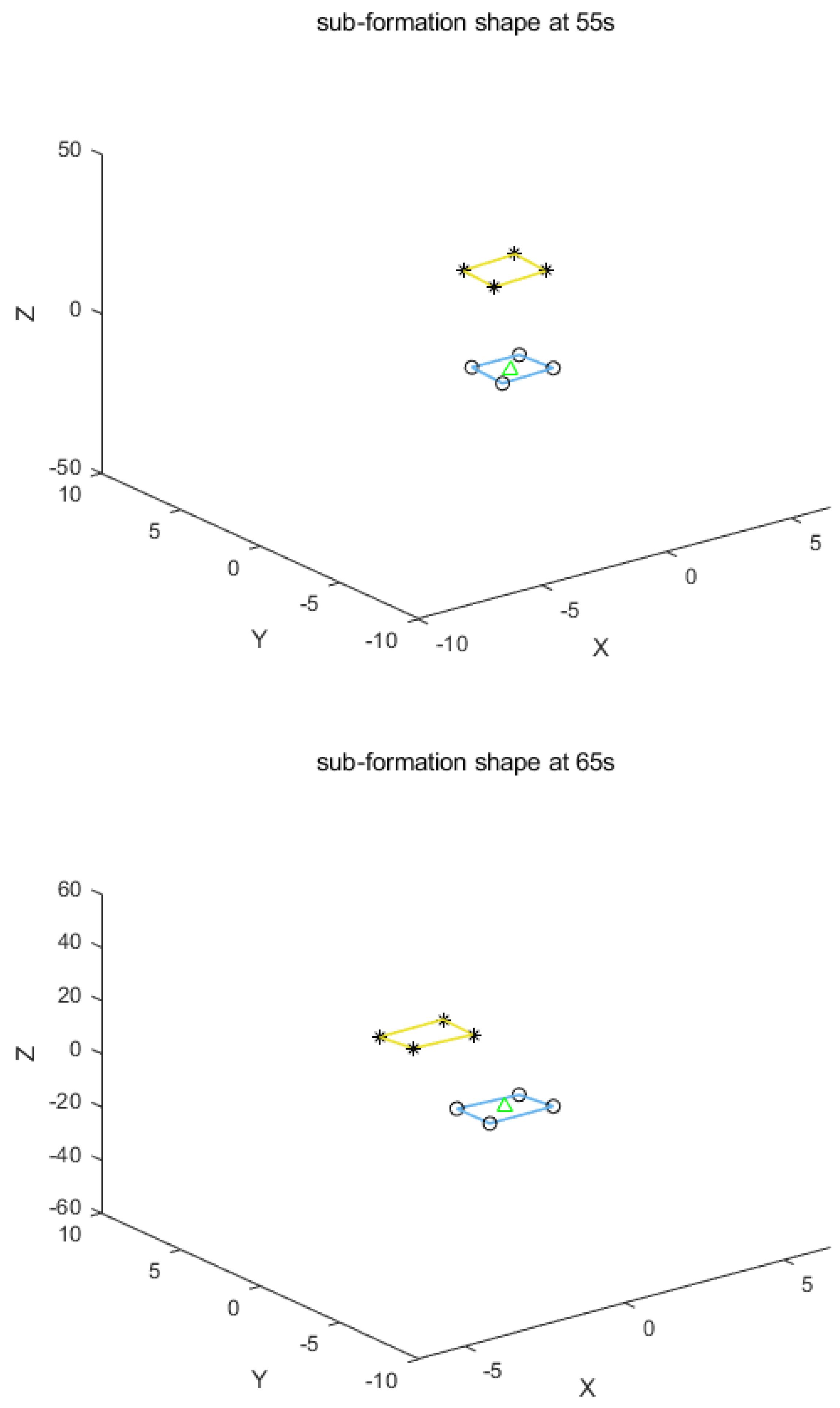
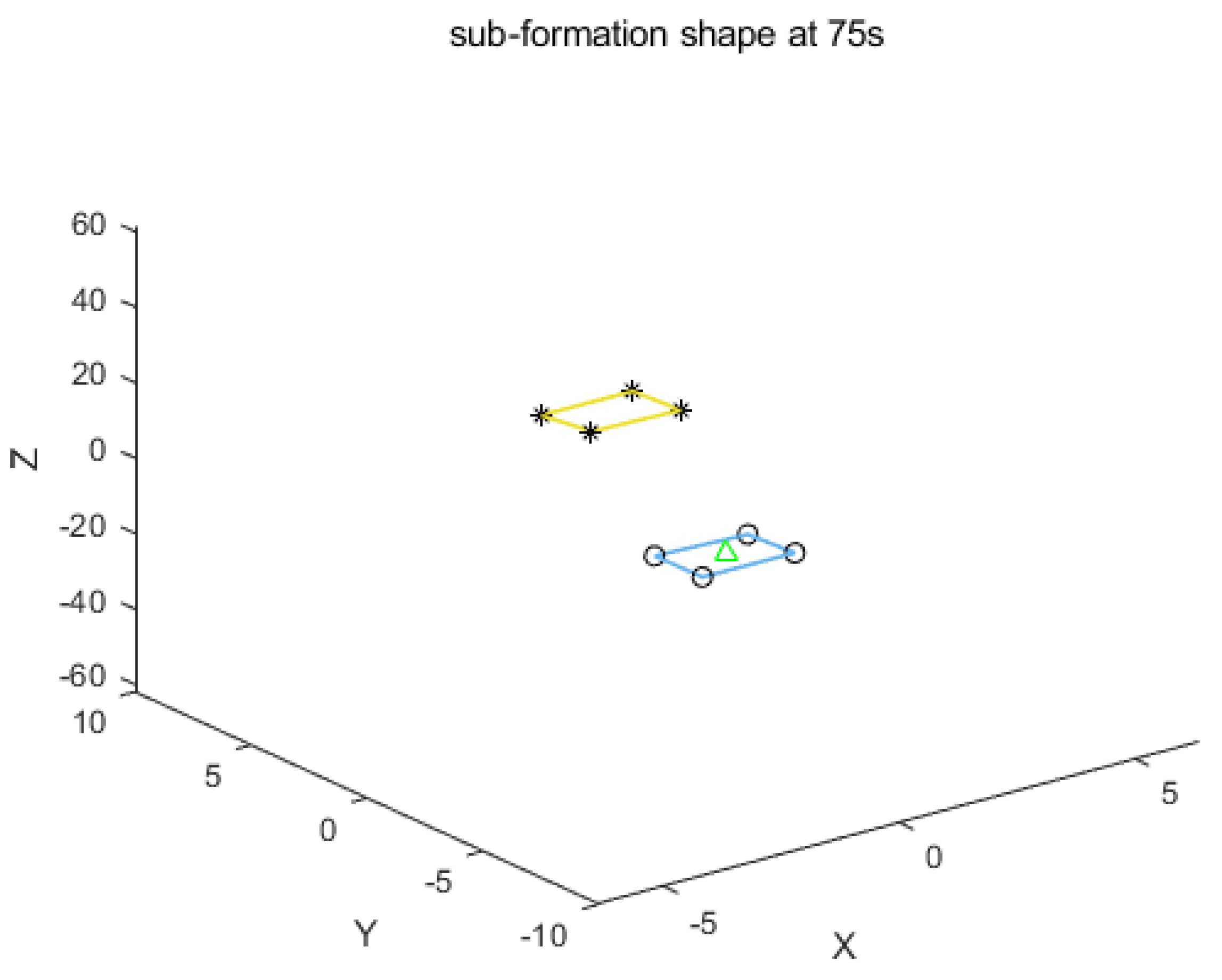
Figure 6. Estimation error of unknown perturbations

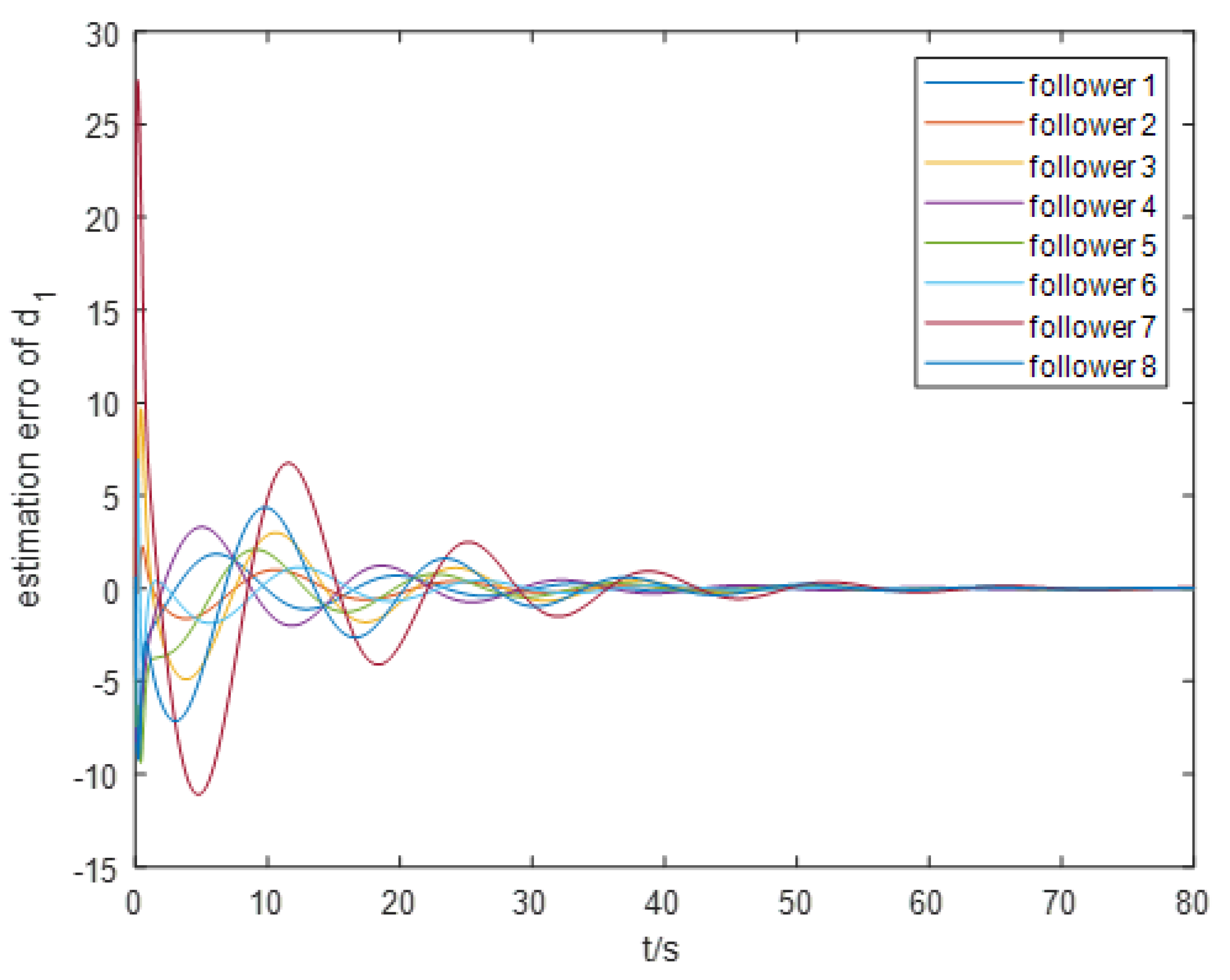
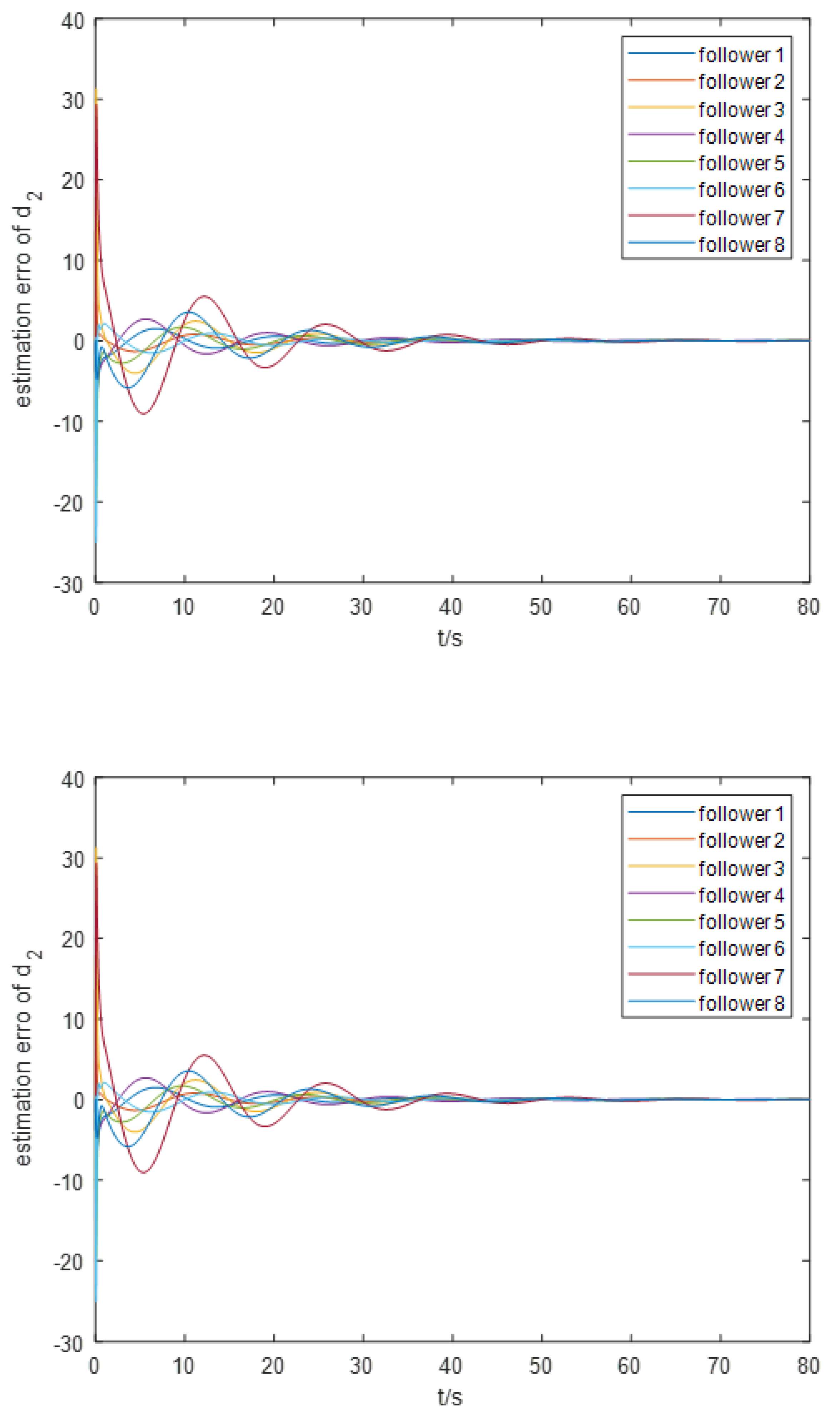
Figure 7. Velocity error convergence for each AUV (from a 3D perspective)

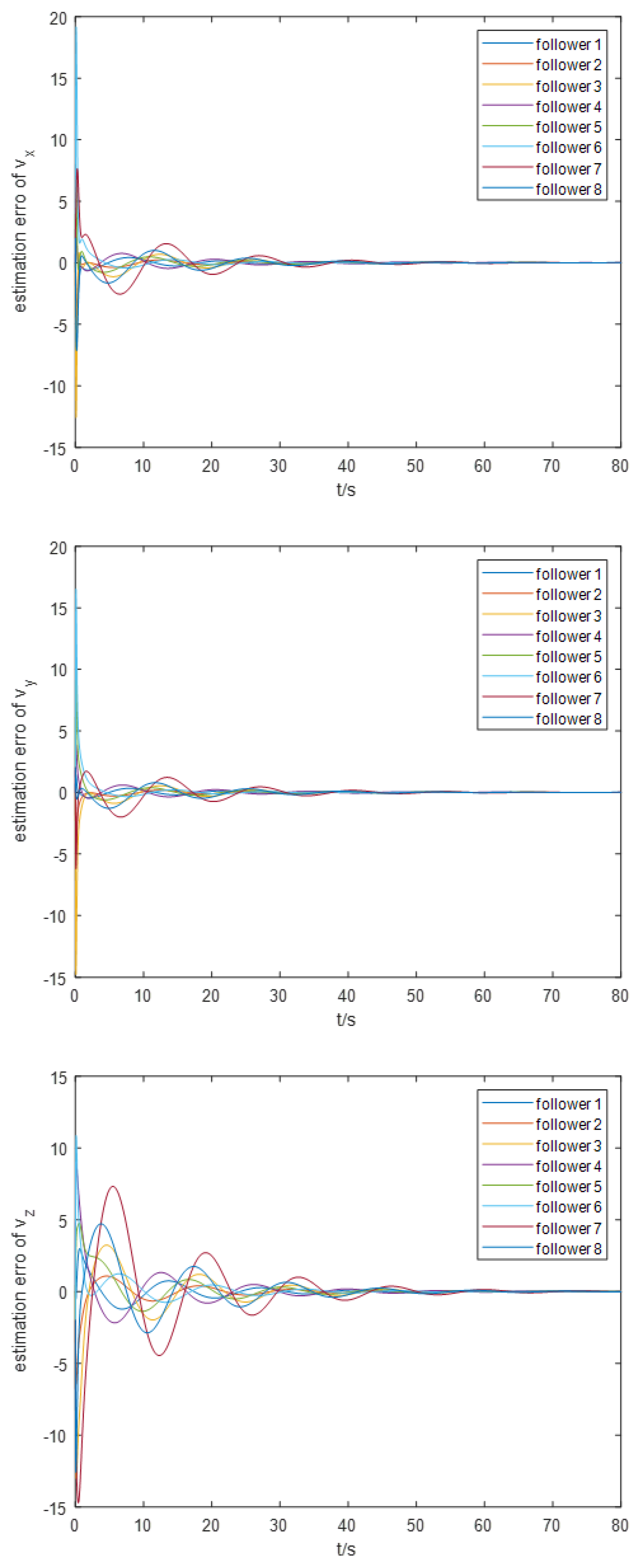
Figure 8. Convergence of position errors for each AUV (from a 3D viewpoint)

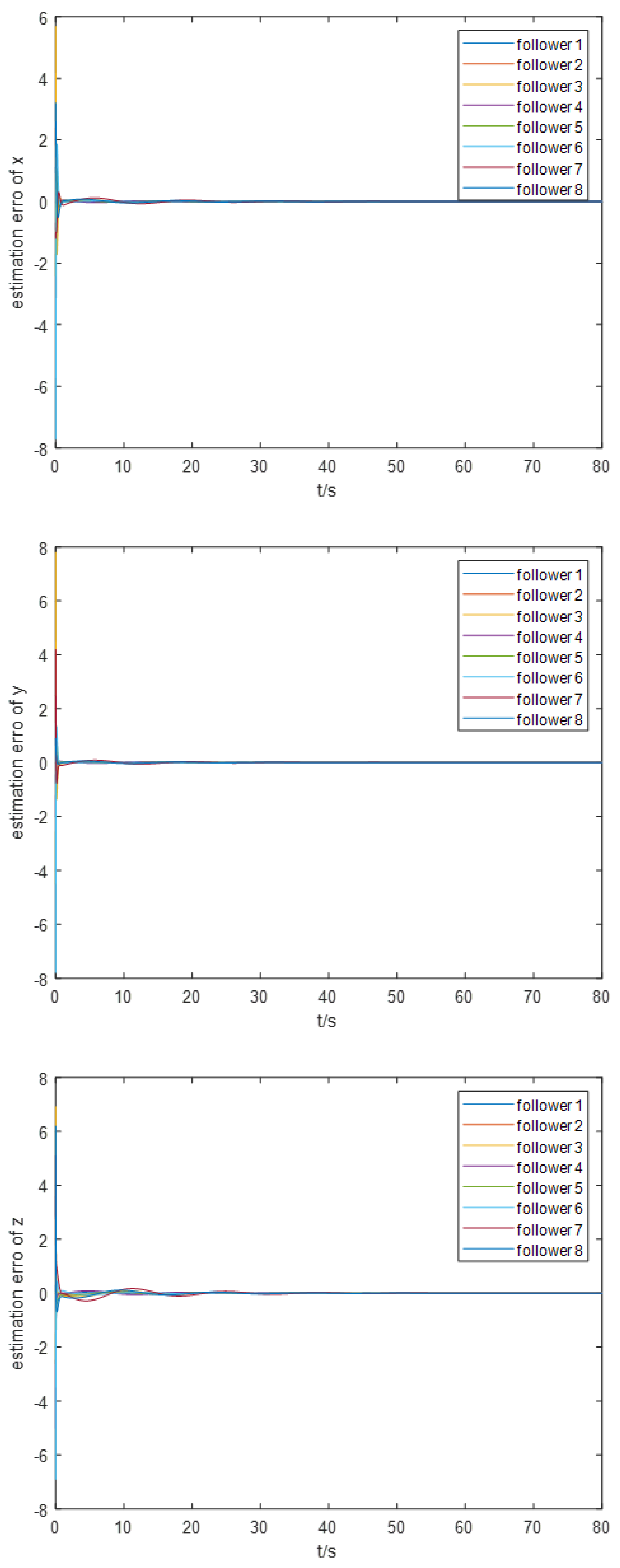
Figure 9. System formation position tracking error (from a three-dimensional perspective)

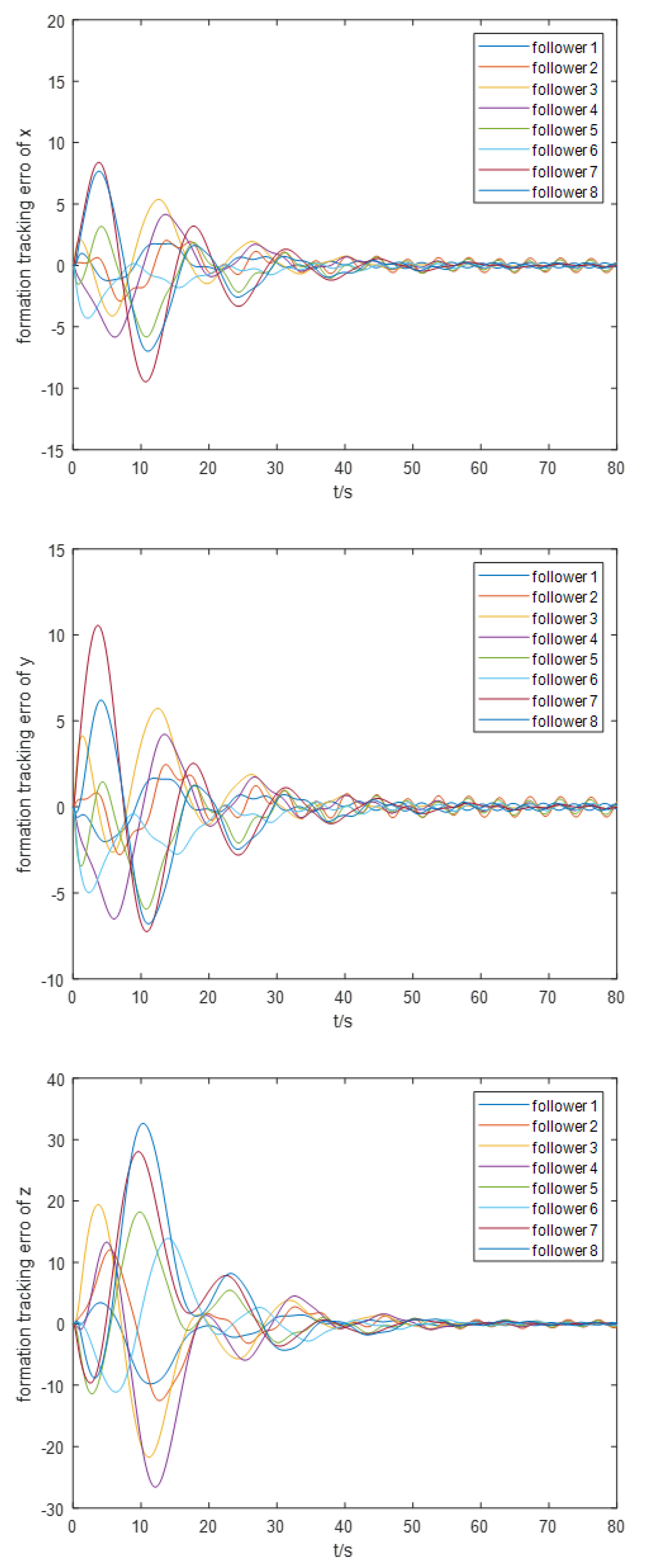
Figure 10. System formation speed tracking error (from a three-dimensional perspective)

Disclaimer/Publisher’s Note: The statements, opinions and data contained in all publications are solely those of the individual author(s) and contributor(s) and not of MDPI and/or the editor(s). MDPI and/or the editor(s) disclaim responsibility for any injury to people or property resulting from any ideas, methods, instructions or products referred to in the content.

© 2024 by the authors. Licensee MDPI, Basel, Switzerland. This article is an open access article distributed under the terms and conditions of the Creative Commons Attribution (CC BY) license (http://creativecommons.org/licenses/by/4.0/).

Copyright: This open access article is published under a Creative Commons CC BY 4.0 license, which permit the free download, distribution, and reuse, provided that the author and preprint are cited in any reuse.

MDPI Initiatives

Important Links

Choose an area of interest and we will send you notifications of new preprints at your preferred frequency.

Disclaimer

Event-Triggered Two-Part Separation Control of Multiple Autonomous Underwater Vehicles Based on Extended Observer

Abstract

1. Introduction

2. Signed Digraph

3. Problem Formulation

4. Expanded State Observer Design Scheme

5. Event-Triggered Control Design Scheme

5.1. Multi-AUV System Two-Part Formation Separation Control

5.2. Design of control inputs and system steadiness

5.3. Design of Trigger Functions and Proof of No Zeno Behavior

6. Simulation Results

7. Conclusion

References

MDPI Initiatives

Important Links

Subscribe