
Submitted:
23 August 2024
Posted:
28 August 2024
You are already at the latest version
Abstract
Recent research has drawn attention to the ambiguity surrounding the definition and learnability of Out Of Distribution (OOD) recognition. The term "Out of Model Scope" (OMS) detection provides a clearer perspective, although the original problem remains unsolved. The ability to detect OMS inputs is particularly beneficial in safety-critical applications such as autonomous driving or medicine. By detecting OMS situations, we not only enhance the system's robustness but also prevent it from operating in unknown and unsafe scenarios. In this paper, we introduce a novel approach for OMS detection that combines three sources of information: 1) the original input, 2) the latent feature space extracted by an encoder, and 3) the synthetic data generated from the encoder's latent feature space. We demonstrate the effectiveness of combining original images and synthetically generated images against adversary attacks in the computer vision domain. We achieve results comparable to other state-of-the-art methods and demonstrate that any Encoder can be integrated into our pipeline in a plug-and-train fashion. Our experiments further evaluate which combination of the Encoder's features works best in order to discover OMS samples and highlight the importance of a compact feature space for the training of the Generator.
Keywords:
Out of Distribution (OOD) Recognition
; Safety-Critical Applications
; Generator as Distribution Approximator
; Robustness of Computer Vision Systems
1. Introduction And Motivation
One of the key factors contributing to the success of deep learning in computer vision is its ability to learn intricate patterns directly from the training data, eliminating the need for manual feature engineering. However, deep learning models are susceptible to overfitting [1] and their performance may degrade when faced with data that lie outside of the training set’s distribution [2].
A neural network trained on images of handwritten digits illustrates this issue: while some implementations [3] achieve near-perfect recognition rates on test data, in real-world scenarios [4] where the inputs are unbounded or uncontrolled [5], there is no guarantee that the images will belong to the same distribution as the training data. In this example, how would a network react to an image of a human? It would classify it as one of the 10 digits. A more tangible example would be autonomous driving, specifically when the car encounters an unknown traffic sign or has to operate in a previously unseen environment. In these cases, there is a need to develop and deploy a Monitoring function which recognizes Out-of-Model Scope inputs and reacts accordingly.
We present a novel perspective on the concept of Out-of-Model Scope [6] inspired by the validation processes described in the Safety of the Intended Functionality (SOTIF) norm [7] and in ISO 26262 [8]. We shed light on critical considerations for enhancing the robustness and reliability of Machine Learning (ML) systems deployed in the computer vision domain. To the best of our knowledge, there is no norm prescribing a specific method for detecting an OMS sample. The implementation of State-Of-The-Art (SOTA) monitors therefore varies and consists of hard-coded boundary binary classifiers that use features extracted from different layers [9], input images, or a combination of both [10]. Our approach aims to incorporate diverse information processed during the prediction phase, as can be seen in Figure 1. We refer to the monitored model as the Encoder and the approximated inverse version of its IMS distribution as the Generator. The detection based on the input images, generated images, and latent feature representations is solved by a learnable Monitor. Throughout this article, we will use the terms "OMS detection" and "OMS monitoring" interchangeably.
Our contributions in the domain of the OMS detection are as follows:
- We describe the theoretical background of OMS detection incorporating a generator of synthetic images.
- We devise a novel multi-input OMS detection pipeline that facilitates monitoring of any pre-trained classifier.
- We demonstrate the robustness of our method against distributional shifts and adversarial attacks.
- Through an ablation study, we evaluate the sensitivity of the OMS monitor to the various inputs.
- We show that our pipeline achieves SOTA results in the computer vision domain.
2. Related Work
2.1. Functional Safety Versus Computer Vision
For practical reasons, the objective of our contribution is aligned with industry norms. As mentioned in the introduction, the uncertainty of machine learning models brings a potential risk in real-world applications. We therefore consider the definitions and processes described in EN IEC 61508 [11] which define a general clustering of safety components in the Safety-Integrity-Level (SIL). On the other hand, the functional safety norm ISO 26262 [8] defines guidelines that minimize the occurrence and severity of hazardous situations related to components’ malfunction or failure. Furthermore, the ISO PAS 21448 [7], also referred to as SOTIF, which builds upon ISO 26262, extends the development process by addressing potential risks in situations where a system could operate incorrectly or unsafely.
The detection of OMS falls within the scope of SOTIF [7]. Nevertheless, the OMS detection pipeline presented in this paper is derived from the concept of hardware (HW) malfunction detection described in ISO 26262 [8]: in the event of a HW failure, the objective is to transition the system to a safe state and enable the operator to maintain control. To achieve this, the safety-critical function and its inverse implementation are monitored by the plausibility function, as highlighted in Figure 2. The implementation of such software (SW) measures reduces the risk of potential undetected malfunctions to a predefined and acceptable level [8].
In Computer Vision (CV), and particularly in deep learning, lossy information compression (Pooling Layers and activation functions) prevents the direct implementation of an inverse function. Additionally, in real-world conditions, the monitoring function must contend with the uncertainty of the monitored model, which is caused either by the model’s limited generalization capabilities [12], or by missing features in the training data [2]. These factors led to the design of a monitoring function [13] based on hard boundaries. The Monitor’s role is to detect the scope in which the model operates safely. Although the Monitor can predict whether the input belongs to the known data distribution, the uncertainty of the OMS detection persists [14].
2.2. OOD and OMS
The terms "Out of Distribution" and "Out of Model Scope" are often used interchangeably, but their definitions vary [15]. In this work, we adopt the definitions and guidelines provided by [6].
2.2.1. Out of Distribution
Let us consider a machine learning task on a domain , such as classification or detection, defined by an oracle function . The oracle function maps points from the task domain to their corresponding ground truths . Using the oracle function , we can define the OOD scope and OMS of any domain. We denote the operational domain as data points . Considering the predefined OOD settings, we assume that the data follows a probability distribution where
Given a new input instance , our goal is to determine whether it originates from the same distribution or if it resides outside of this distribution. This leads to the formulation of an out-of-distribution monitor given by
2.2.2. Out of Model Scope
Referring to the nomenclature established in Section 2.2.1, we define the model scope as follows:
where f denotes the deployed model.
We aim to develop an OMS monitor capable of identifying all data points that fall outside the model scope . This monitor function is defined as follows:
As can be seen in Equation 2, OOD detection focuses on distinguishing among an infinite number of probability distributions within the domain and a specific In Distribution . However, capturing all boundaries within a CV domain is only possible if the condition is fulfilled [14]. Proposed solutions for OOD detection in a stochastic environment are consequently vulnerable to adversarial attacks and shifts within the ID, as demonstrated in [16]. Furthermore, the definition of OOD can be significantly influenced by the domain and definition of the machine learning task. These ambiguities led to the implementation of various monitoring functions and the attainment of diverse results, as shown in [17].
In contrast to OOD, the definition of OMS provides a more precise and consistent framework for detecting samples that our model should not classify or make predictions on, as they are not drawn from . The conditions for learnable OMS remain the same as for OOD [14]; nonetheless, its clearer definition eliminates the need to differentiate between outlier detection [18,19], anomaly detection [20,21], novelty detection [22], and the open-set recognition problem [23,24], as was the case with OOD. Due to these findings, we will focus only on OMS detection instead of OOD detection. Based on the OMS Monitor definition in Equation 4, our OMS encompasses both covariate and semantic shifts, as well as adversarial attacks. These distribution shifts can be introduced into the training data through various means, such as:
- Covariate shift: altering certain image aspects, such as brightness, to a degree that causes the classifier to fail.
- Semantic shift: introducing semantic content that has not been reviously encountered in our domain .
- Adversarial attack: incorporating malicious perturbations in the input data, imperceptible to human eyes.
2.3. Oms Metrics And Monitors
Although the monitors and metrics discussed in this chapter were originally developed for detecting OOD samples, they can also be utilized for OMS detection [6]. Moreover, it is common to cluster OOD detection methods based on the used inputs. As highlighted in Figure 1, the following possibilities are available:
- feature-based
- probability-based
- logit-based
- feature and logit-based
Our method is a novel generative approach utilizing features and logits.
2.3.1. Metrics
Among the possible feature-based methods, the distance between any point within the operational domain and the ID distribution , called the Mahalanobis distance (MAHA), is the most frequently used. Introduced by P.C. Mahalanobis [25], the Mahalanobis distance was further employed by Lee et al. [26] through a Gaussian discriminant analysis applied to the softmax layer. Lee et al. discovered that abnormal samples are better represented in the feature space of Deep Neural Networks (DNNs) rather than the "label-overfitted" output space of softmax-based posterior distribution, as demonstrated in earlier studies [27,28].
The Max Softmax Probability (MSP) method, pioneered by Hendrycks and Gimpel [13], established OMS detection based on the hypothesis that correctly classified examples should exhibit higher probability compared to other classes. This involved determining a statistical threshold for a binary classifier using a validation set. On top of this work, Liang et al. built their ODIN (Out-of-Distribution detector for Neural Networks) system [29]. They used temperature scaling to maximize the discriminability of the softmax outputs for In- and Out-Of-Distribution images. Hendrycks et al. further focused on large-scale datasets anomaly detection and proposed using the negative of the maximum of the un-normalized logits for an anomaly score, which they called MaxLogit [30].
As pointed out by Liu et al. [24], relying solely on softmax probabilities led to high confidence for misclassified samples. Liu et al. therefore incorporated an energy-based score that is theoretically aligned with the probability density of the inputs and less susceptible to overconfidence.
2.3.2. Monitors
The Outside-the-Box method, introduced by Henziger et al. [23], addresses novelty detection by employing a monitor on top of the arbitrary hidden layers of a pre-trained classifier. During training, the method samples class-related responses and clusters them, thus improving monitor accuracy. Novelties are recognized using a set of box abstractions that determine whether a new data point is inside or outside of the projected box.
Motivated by activation patterns analysis, Sun et al. [31] noted that activations of OMS samples differ significantly from those of In Model Scope samples. Their Rectified Activation (ReAct) method further showed that gathering activations from other than the penultimate layer does not enhance accuracy, as early layers capture less distinctive features.
The latter statement, asserted by [31], was negated by Lin et al. [9], who evaluated the possibility of detecting an OOD sample from different intermediate layers. They proposed a new energy-based score to dynamically terminate an early exit during inference. They picked their early exit based on the number of bits needed to encode the compressed image, consequently proving on many datasets that less complex OMS inputs can also be reliably discovered from the early layers.
2.3.3. Other Evaluation Metrics
Class imbalances and other non-uniformities in the number of False Positives (FP) and False Negatives (FN) must be considered during the evaluation of any classifier. To address this, the Area Under the Receiver Operating Characteristic (AUROC) [32] is frequently used in conjunction with F-score. AUROC evaluates the True-Positive Rate (TPR) against the False-Positive Rate (FPR), where the TPR is calculated as and the FPR analogously as , where TN stands for True Negative samples. Nonetheless, as mentioned in [13], AUROC may not be suitable when the positive and negative classes have notably different base rates. In such cases, the Area Under the Precision-Recall curve (AUPR) is preferred, as it adjusts for the varying positive and negative base rates. Another metric we use to combat class imbalance in the data is the balanced accuracy where is the true positive rate as defined before and the True Negative Rate (TNR) is given by From now on, we refer to accuracy in OMS domain as balanced accuracy.
3. Oms Monitoring Pipeline
All components of the OMS monitoring pipeline are depicted in Figure 3. Our primary goal is to enhance the robustness of OMS Detection by providing multiple inputs to our OMS monitor. The weights of the Encoder E represent the feature space extracted from the operational domain , which, in return, represents the IMS distribution . The Generator G produces reconstructed synthesized images based on a combination of latent features z. Ideally, if the input sample x belongs to the model scope , G generates an image from the same distribution. On the other hand, when an OMS input is presented, the generator combines different features based on the Encoder’s latent feature representation z in the generated image. This representation z is extracted by a Latent Space Wrapper L and can contain information from different layers of the Encoder and its softmax prediction . In the last step, the OMS binary classification is addressed by a multi-input OMS monitor . This monitor receives three inputs: the original input image x, the reconstructed image , and the latent feature representation z. Conceptually, our OMS monitor can be seen as a mapping . The description of the inference process is presented in Algorithm 1.
Based on the theoretical and practical expertise we gathered during experimentation, we have identified that the following properties of the OMS pipeline need to be fulfilled.
- The input space cannot be infinite, as described in [14].
- The Generator should have high reconstruction capability for samples within the Encoder’s scope and lose this ability for samples outside the scope : to achieve this, during the generator’s training, we minimize the classification loss between the Encoder’s prediction on the original and generated images from the model scope.
- To be able to compare the contribution of our multi-input OMS pipeline, we investigate the performance fluctuation of the Monitor with the ablation study.
- To increase the robustness we use Dropout directly on the inputs provided to the OMS monitor, namely x,, and z.
| Algorithm 1 OMS Monitor during inference. |
|
In general, the Encoder can be any deep neural network that has been trained on the operational domain ; its implementation must allow access to intermediate layers. The Generator has to follow an inverse information flow with respect to the Encoder. In our case, the generator produces synthetic images with the same resolution as the input image x. This allows us to directly evaluate the image fidelity with the Fréchet Inception Distance (FID) [34] and the Inception Score (IS) [35]. There are no further constraints on the implementation of the Generator, and its architecture can be similar to Generative Adversarial Networks (GANs) [36], or Latent Diffusion models [37]. What distinguishes our approach from our predecessors’ is that the OMS monitor contains learnable parameters and receives synthetic images from the approximated density function of the Encoder, namely: the Generator.
4. Experiments
The evaluation setup of our experiment was inspired by [6,9]. However, instead of using pre-trained networks, we explore the influence on the OMS performance by training custom ResNet models with a different number of parameters and layers.
4.1. Ims And OMS Datasets
We chose the CIFAR-10 [38] as our initial dataset, following common practice in the OOD and OMS community. We split all datasets uniformly: 70% were used for the training set, 20% for validation, and the remaining 10% for testing purposes.
The OMS dataset consists of semantic shifts, covariate shifts, adversarial attacks, and FP samples. We built the set of semantic shifts using publicly available datasets, namely MNIST [39], fashion-MNIST [40], k-MNIST [41], SVHN [42] and DTD [43]. To test our pipeline’s robustness against covariate shifts in the data, we introduced various modifications to the original CIFAR-10 dataset. These modifications were applied until the Encoder failed to recognize otherwise correctly classified IMS samples. The applied modifications included blurring, brightness adjustments, image rotations, and noise addition. Lastly, we introduced imperceptible malicious perturbations to the IMS data, also known as adversarial attacks [44]. These perturbations are designed to be undetectable by human observers. Our approach involved leveraging the Fast Gradient Sign Method (FGSM) [45], Projected Gradient Method (PGD) [46], DeepFool [47] and AutoAttack [48]. The implementation in the Torchattacks [49] library was used in our case. The FPs samples, which are identified after the training of the Encoder is completed, form a default OMS dataset. Consequently, the identified TPs form the IMS () dataset. A selection of random samples and transformations from all datasets can be seen in Figure 4. Furthermore, a summary of all methods that were used to construct the OMS datasets is highlighted in Table 1.
4.2. Training
The OMS monitoring pipeline consists of four main components: the Encoder E, the Generator G, the OMS monitor O, and the Latent Space Wrapper L. Each component is trained independently, which ensures a plug-and-train monitoring system that can be applied to any pre-trained Encoder (e.g. a ResNet).
4.2.1. Encoder
To establish the foundation for the IMS dataset, we commenced with the training of the Encoder, which defines the IMS dataset as per Equation 3. We employed ResNet models [50] with 18, 34, 50, and 101 layers, leveraging the CIFAR-10 dataset divided by the guidelines outlined in Section 4.1. Each model underwent training with the Adam optimizer [51], for a total of 500 epochs, employing a learning rate of and following a cyclic learning rate scheduler, all while utilizing a batch size of 1024. The Categorical Cross Entropy was used as loss function. Additionally, we applied various data augmentation techniques available in PyTorch [52], including random horizontal flipping, random cropping, and random affine transformations.
Many OMS detection methods assign a score to an input sample based on its representation in the feature space. Given the infinite variations in OMS data, we have to rely on the IMS feature space generated by our Encoder. Should this feature space representation of our IMS data lack relevance, it may falsely contribute to the detection of OMS examples. As a result, we applied regularization techniques related to the latent feature space. This involved implementing a dropout mechanism with a probability of 0.2 for zeroing out and incorporating a Spatial Feature (SF) regularizer. The SF regularizer calculates both inner and outer cosine class similarities. During training, it maximizes the inner similarity while minimizing the outer similarity. For a visual comparison of the feature spaces before and after regularization, we refer to Figure 5, which showcases the Uniform Manifold Approximation and Projection (UMAP) [53] results.
4.2.2. Generator
Let us start with the theoretical description of the role of our Generator in the example of the vanilla GAN architecture. The GAN architecture is comprised of two main components: the Generator (G) and the Discriminator (D). The Discriminator is trained to differentiate between an original image x and a synthetic image created by the Generator . This is reflected in its loss function: . Concurrently, the Generator aims to produce images that l the Discriminator, optimizing its loss function: . The Generator uses a latent vector z as input, typically sampled from a Normal distribution with mean=0.0 and standard deviation=1.0. During the training, the vanilla GAN model attempts to minimize the KL divergence [54] between the IMS data distribution and the implicit generator data distribution . This often leads to learning instability and difficulty in capturing structural and geometric features [55]. Consequently, this has spurred the development of enhanced GAN architectures such as convolutional GAN [56], Self-Attention GAN [57], BigGAN [58], and Style GAN [59], along with improved training setups like Wasserstein GAN with gradient penalty [55] and spectral normalization [60].
The Generator in our pipeline aims to densely approximate the IMS distribution . Its task is to reconstruct the input x given its latent feature space representation z and the predicted class of the Encoder E. More specifically, the generator learns . It should be noted that during the training with the IMS dataset, we can use y in place of , and thus use . Our goal is to minimize the distance between and ; but instead of using a random noise, we utilize the latent feature space from the Encoder E. Consequently, we minimize the classification loss , where is the Categorical Cross Entropy (CCE) between ground truth label y and the classified generated image . In our case, the representation of z can correspond to the latent feature space of one or more layers. The complete training loss function for the Generator G is detailed in Equation 5.
where denotes the expected value over the probability distribution of the true labels y, C is the number of classes, is a ground-truth indicator, is the predicted probability and is a scaling factor for training stability, empirically set to .
We applied the aforementioned training approach to all three models, WGAN [55], BigGAN [58] and Class Conditional Latent Diffusion Model [37] (CCLDM). To summarize, the following hyper-parameters were explored in terms of image fidelity and contribution to OMS detection:
- generator’s architecture and size,
- dimension of the latent feature space z,
- class/feature-embedding method,
- combination of intermediate layers building the latent feature space z,
- implementation of the latent space wrapper L,
- and integration of a CCE between ground truth label y and the classified generated image.
For the first two GAN-based models(WGAN and BigGAN), we utilized the training loss described in Equation 5 and followed the hyperparameters’ settings from the original papers. In the case of the CCLDM model, the class embedding information was directly concatenated with the denoising parameters and the original image. During the training, the original image, with added noise, was reconstructed and the Mean Squared Error between the original and denoised image was minimized. The main component of the diffusion architecture is the denoising U-Net [61] model.
By incorporating the latent features z extracted by the encoder as class conditioning information, we encourage our generator to synthesize images of the same class with similar features learned during the Encoder’s training. Our hypothesis is guided by the expectation that even in the event of an adversarial attack, where the sample falls outside of the model’s scope, the Generator will still reconstruct an image containing features from the IMS distribution. To achieve this, we explore the hyper-parameter space and evaluate which combinations are the most effective for OMS detection in general.
4.2.3. Latent Space Wrapper
As previously mentioned, we use information from the latent feature space of the Encoder. Since this feature space can stem from any arbitrary deep neural network, we have to devise a mechanism that will aggregate the information from different feature maps of the model and produce a single latent representation z. We deploy a non-trainable approach, by applying Average and Max-Pooling layers directly to the intermediate layers, as well as a trainable approach with convolutional layers with a stride of the size of the kernel. Our Latent Space Wrapper, which adapts to the size of each given layer and whose parameters are tuned during the training of the Generator, can be seen in Appendix in Figure A1.
4.2.4. OMS Monitor
In the final phase, we train the OMS Monitor. The primary task of the OMS Monitor is to perform binary classification based on the similarities between its three inputs. Specifically, the Monitor predicts whether the input from the Encoder is OMS or not.
During the training of the OMS Monitor, we construct the OMS datasets using the methods and combinations described in Section 4.2. It is noteworthy that if we solely consider FPs as OMS examples, the size of the OMS dataset is contingent upon the performance of the Encoder. In scenarios where the Encoder achieves 100% accuracy, the OMS dataset would consist of an empty set of images. This underscores the dependency between the size of the OMS dataset and the performance of the Encoder, thereby justifying the necessity of integrating supplementary OMS data. To address potential issues of dataset imbalance during training, we employ Focal Loss [62] and weight random sampling techniques.
Notably, we do not apply any data augmentation on the IMS dataset. This precaution is to prevent a sample from inadvertently being categorized as OMS. Building on the training setup of the Encoder, we apply Dropout before each Linear Layer, and we use Binary Cross Entropy as the loss function.
4.3. Evaluation of Encoder and Generator
As Encoder, we trained different ResNet models, namely with 18, 34, 50, and 101 layers. All models consist of 4 blocks, which serve as binding points to our Latent Space Wrapper. The accuracy of the Encoders for each dataset is presented in Table 2.
As elaborated in detail in Section 4.2, the generator is trained on the IMS dataset. The highest classification ACCuracy on the generated images , was achieved by the bigGAN model with a latent feature space dimension of 64, combining the features extracted from ResNet34 blocks 1 and output from the softmax layer. This model reached for the training set and for the validation set. Image fidelity and image variance were evaluated by the Frechet Inception Distance (FID) [34] and Inception Score (IS) [35], which correlates well with human judgment [63]. The same model achieved FID of and IS of . To increase the evaluation set and as recommended in the original FID paper, all samples from the IMS dataset were included in the assessment.
The best model of each generator’s architecture can be found in Table 3. As we conditioned the training loss from Equation (5) by , our model finds the optimum between image fidelity and the accuracy of the Encoder. Consequently, our generator achieves lower IS and higher FID scores than reported in the original papers.
As mentioned at the beginning of Section 4.2.2, several hyper-parameters influence the generator’s and consequently the monitor’s performances. The influence of the dimension of the latent feature z on the is highlighted in Figure 6. An ablation study of different combinations of layers further shows that the most relevant features are contained in the deeper layers. As can be seen in Figure 6, a generator trained on combinations of features extracted from multiple layers outperforms a generator that was trained only on features from one specific layer.
Although the highest classification accuracy on CIFAR-10 was achieved by ResNet-34, as highlighted in Table 4, the combination of Generator with ResNet-18 showed similar results in the OMS detection task as the combination with ResNet-34. The deployment of more complex Encoders with a higher number of layers didn’t improve the performance of the Generator. On the contrary, as visible in Table 5, applying dropout during the training of the Encoder improved the Generator’s performance. The final overview presented in the Appendix in Table A2 summarizes all hyper-parameters and techniques related to the Generator’s training.
4.4. Evaluation OMS Detection
In the case of OMS monitor, we deal with a binary classification problem involving the identification of two classes. However, it is a common scenario for the volume of OMS data to be larger than the IMS data, both in real-world applications and experimental setups [64]. As written in Section 2.3, to address this issue, we employ metrics that consider a trade-off between TPs and FPs and calculate the balanced accuracy instead of vanilla accuracy.
As mentioned in Section 4.2, we train the OMS monitor on each IMS and OMS training set presented in Table 1 and validate it on all the IMS and OMS validation and test sets. In our experiment, we explore various combinations of OMS datasets to discern the individual impact of each dataset on the OMS detection instances. Achieved results are presented in Table 7.
4.5. Ablation Study Of The OMS Monitor
Ablation studies in machine learning involve systematic evaluation of a model by removing or modifying its components to understand their impact on its performance. In the context of our OMS Monitor, the key elements under consideration are the original input x, the latent feature representation z, and the generated image , all of which serve as inputs to the OMS monitor.
The results, as presented in Table 8, show the contributions of each input to the overall OMS detection. The accuracy drops by after removing the original input image x, proving that the primary source of relevant information for the OMS monitor still lies within the original input data. On the other hand, incorporating the feature space and generator increases the overall classification accuracy by approximately . This subtle improvement can be explained by insufficient approximation of the IMS distribution . Namely, the best bigGAN model achieved an accuracy of on the IMS training set. Images identified as FP by could be considered for removal from the original IMS training set. However, this action would only superficially boost the to , but shrink the valid IMS samples training set, thereby impairing the Monitor’s ability to generalize.
5. Conclusions and Future Work
Our novel OMS Monitoring pipeline represents an advancement in the development of functional safety monitors. It effectively detects samples that were not part of the training setup, preventing actions that could lead to severe consequences. As demonstrated in Section 4.4, our OMS Monitoring pipeline, inspired by the HW-Malfunction detection, achieves a balanced accuracy of on OMS samples from previously unseen test sets. Furthermore, it exhibits the highest AUROC, , among all evaluated monitors and metrics. As can be seen in Table 7, our pipeline excels in detecting adversarial attacks, which were designed to deceive the potentially safety-critical Encoder. The overall detection accuracy was achieved by incorporating OMS distribution shift methods during OMS Monitor training. However, it is important to note that detecting false positives, which were excluded from the original dataset, remains the most challenging aspect of OMS detection. This behavior is not unique to our monitoring pipeline but is consistent across state-of-the-art methods, as shown in Table 10. Our method achieved the best results quantified by Area Under the Receiver Operating Characteristic, and the probability that a negative (OMS) example is misclassified as positive (IMS), namely FPR95TPR. Our weaker performance in AUPR compared to the current SOTA methods can be explained by the optimization process of the OMS monitor, via binary cross entropy, which rewards both TP and TN. This dichotomy can result in a slight decrease in precision, as can be seen in Table 9.
In Section 4.3 we thoroughly discussed the contribution of the Generator to the OMS Monitoring pipeline. The approximation of the IMS distribution of the Encoder improved mainly due to the incorporation of the classification loss on the reconstructed images and by utilizing the Latent Space Wrapper. Consequently, the OMS training improved in stability as well as in accuracy. A notable drawback of using the Diffusion architecture as a Generator throughout our experiment was a high inference time caused by an iterative diffusion process. Even though the FID and IS scores of the diffusion model were better than those of the bigGAN, the bigGAN model achieved the highest which, as mentioned in Section 4.2.2, is more relevant in the context of the OMS detection task.
To summarize the key takeaways, our OMS Monitoring pipeline allows the integration of any pre-trained Encoder, regardless of the working domain. We demonstrated the potential of a robust OMS sample detection, where the main focus was laid on the utilization of the Generator as a universal approximator of the Encoder’s latent space. Due to all our improvements the OMS detection pipeline achieved high accuracy in detecting various Adversarial Attacks, . We hope that this potential will open doors to further topics and future work, namely:
- Adjustment of our OMS detection pipeline to other tasks in computer vision and other fields of machine learning, such as Natural language processing.
- Research of a possible approximation of the intermediate encoders’ layers and investigation of end-to-end training which we found based on the definition of IMS, currently not applicable.
Author Contributions
Conceptualization, V.D.; methodology, V.D. and B.S. and M.H.; software, B.S. and V.D.; validation, B.S., V.D. and M.H.; formal analysis, V.D.; investigation, V.D.; resources, V.D.; data curation, B.S. and V.D.; writing—original draft preparation, V.D.; writing—review and editing, V.D., B.S., M.H.; visualization, V.D. and B.S.; supervision, V.D. and M.H.; project administration, V.D.; funding acquisition, V.D. and M.H.
Funding
Not applicable
Institutional Review Board Statement
Not applicable
Informed Consent Statement
Not applicable
Data Availability Statement
All data supporting reported results can be found on:
- Throughout our work we used publicly available datasets which are correctly cited.
- FashionMNIST: https://github.com/zalandoresearch/fashion-mnist
Acknowledgments
Computational resources were provided by the e-INFRA CZ project (ID:90254), supported by the Ministry of Education, Youth and Sports of the Czech Republic. This work was supported by a grant from the University of West Bohemia, project No. SGS-2022-017.
Conflicts of Interest
The authors declare no conflicts of interest.
Abbreviations
The following abbreviations are used in this manuscript:
| OOD | Out Of Distribution |
| OMS | Out of Model Scope |
| IMS | In Model Scope |
| SOTIF | Safety of the Intended Functionality |
| SOTA | State-Of-The-Art |
| SIl | Safety-Integrity-Level |
| HW | HardWare |
| CV | Computer Vision |
| MAHA | Mahalanobis distance |
| DNN | Deep Neural Network |
| MSP | Max Softmax Probability |
| ODIN | Out-of-Distribution detector for Neural Networks |
| AUROC | Area Under the Receiver Operating Characteristic |
| AUPR | Area Under the Precision-Recall curve |
| FP | False-Positive |
| FN | False-Negative |
| TN | True-Negative |
| TNR | True Negative Rate |
| TPR | True Positive Rate |
| GAN | Generative Adversarial Networks |
| FSGM | Fast Gradient Sign Method |
| PGD | Projected Gradient Method |
| UMAP | Uniform Manifold Approximation and Projection |
| CCE | Categorical Cross Entropy |
| CCLDM | Class Conditional Latent Diffusion Model |
| WGAN | Wasserstein-GAN |
| IS | Inception Score |
| FID | Frechet-Inception Distance |
Appendix A
Appendix A.1. Latent Space Wrapper
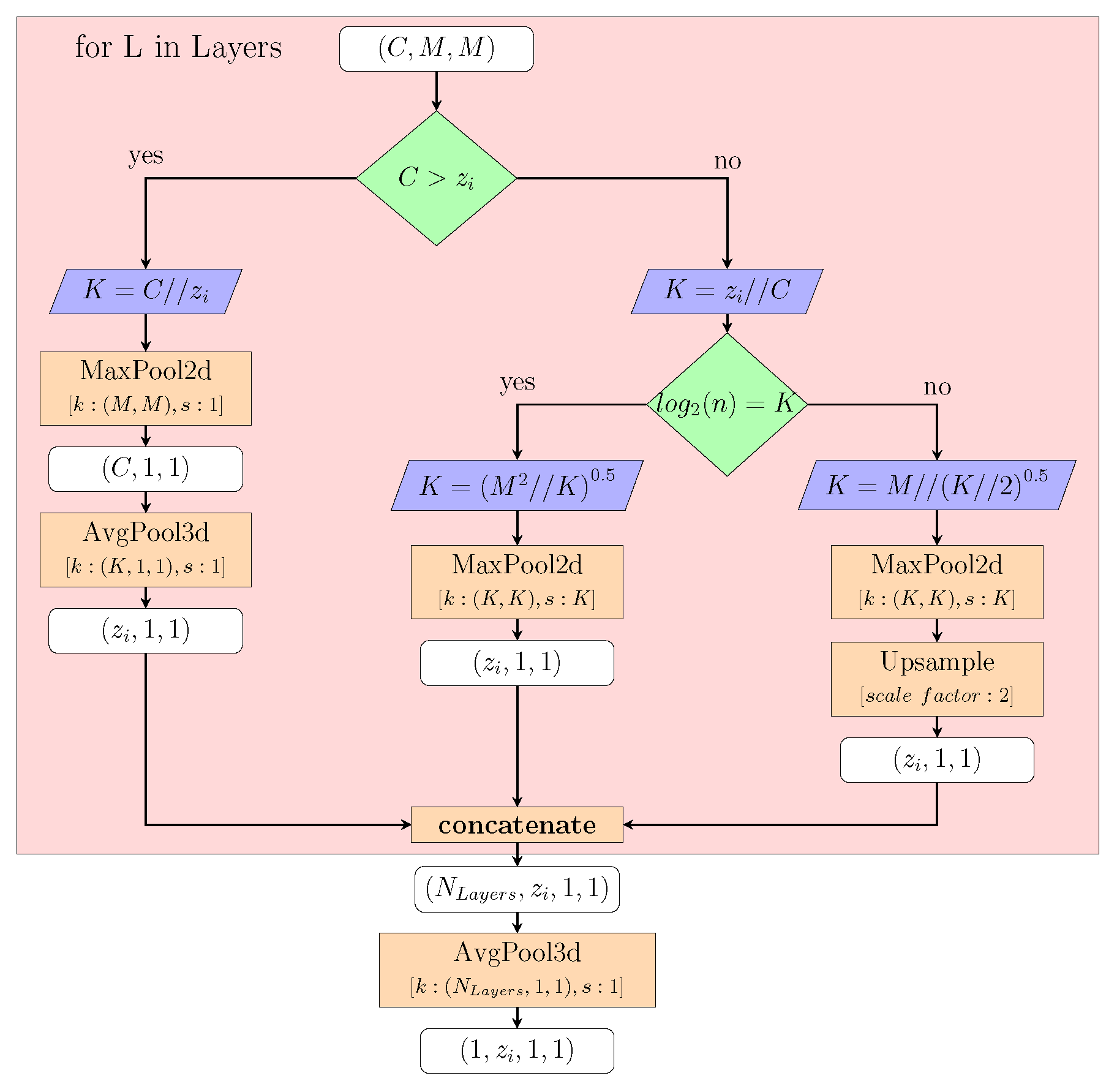
Figure A1 depicts a non-trainable computational graph. Within the computational process, we scale the inputs of each layer to the dimension of the tensor z with a given feature map of dimensions . The left part of the graph depicts the latent feature space reduction through Average and Max-Pooling layers. The right branch gives an example of applied layers when the number of channels C is smaller than the required feature space dimension of z. In this chart, operations such as up-scaling and reshaping, which are necessary for achieving the desired output tensor shape, are not visualized. The trainable Wrapper replaces the Maximum Pooling layers with Convolutional layers and uses the calculated K as kernel size and stride.
Figure A1.
This diagram represents a computational graph of a non-trainable latent space wrapper.
Appendix A.2. Performance of Generator
During training, the Generator G minimizes the reconstruction loss between the original and the generated image . This implies that the weights capture an approximated inverse function to our model E. Consequently, the reconstructed image is the outcome of , where generally represents a combination of aggregated feature spaces from various layers. As we want to enhance the robustness of our OMS detection pipeline by the reconstructed image from the Generator, we have to ensure its best performance. We therefore conducted several additional experiments with learnable and non-learnable latent space wrappers as can be seen in Table A1. The most robust performance was achieved by extracting the features via maxPool layer. All techniques and their influence are further summarized and listed in Table A2.

Table A1.
Variations of learnable and non-learnable latent space wrapper only for the bigGAN generator, showing the differences in , and .
Table A1.
Variations of learnable and non-learnable latent space wrapper only for the bigGAN generator, showing the differences in , and .
| ↑IS | ↓FID | ||
| avgPool | 7.87 | 29.22 | 90.78 |
| maxPool | 7.92 | 28.04 | 91.96 |
| learnable | 6.89 | 32.07 | 78.45 |
Table A2.
Summary of all hyper-parameters and techniques and their influence on the generator’s training. FS stands for Feature Space.
Table A2.
Summary of all hyper-parameters and techniques and their influence on the generator’s training. FS stands for Feature Space.
| Method / Hyper-parameter | Reference | Reasoning | |
| Encoders depth | Small | Table[4] | Deploying more complex ResNet models on the CIFAR-10 dataset didn’t improve the accuracy of the encoder, nor did it enhance the performance of the decoder. |
| Encoders FS regularization | Middle | Table[5] | Training with Dropout and Feature regularization influences FS’s compactness and consequently improves the Generators’ training performance. |
| Generators Architecture | High | Table[3] | Almost similar results were achieved by the bigGAN model and Stable Diffusion model with latent class embedding. Compared to bigGAN, the WGAN achieved lower performance by 21%. |
| FS dimension | Middle | Figure[6a] | Grid search method settled around the dimension of size 64. Smaller and higher feature space dimension results in lower . |
| FS layers combination | Middle | Figure[6b] | Combination of features from more than one and deeper layers results in higher . |
| Trainable Latent Wrapper | Small | Table[A1] | The best results were achieved by finetuning the latentwrapper with Max Pooling Layers. The combination with trainable Conv2d layer didn’t improve the . |
References
- Srivastava, N.; Hinton, G.; Krizhevsky, A.; Sutskever, I.; Salakhutdinov, R. Dropout: a simple way to prevent neural networks from overfitting. The journal of machine learning research 2014, 15, 1929–1958. [Google Scholar]
- Der Kiureghian, A.; Ditlevsen, O. Aleatory or epistemic? Does it matter? Structural safety 2009, 31, 105–112. [Google Scholar] [CrossRef]
- Byerly, A.; Kalganova, T.; Dear, I. No routing needed between capsules. Neurocomputing 2021, 463, 545–553. [Google Scholar] [CrossRef]
- Rao, Q.; Frtunikj, J. Deep Learning for Self-Driving Cars: Chances and Challenges. In Proceedings of the 2018 IEEE/ACM 1st International Workshop on Software Engineering for AI in Autonomous Systems (SEFAIAS), 2018, pp. 35–38.
- Vaze, S.; Han, K.; Vedaldi, A.; Zisserman, A. Open-Set Recognition: a Good Closed-Set Classifier is All You Need? In Proceedings of the International Conference on Learning Representations, 2022.
- Guérin, J.; Delmas, K.; Ferreira, R.; Guiochet, J. Out-of-distribution detection is not all you need. In Proceedings of the Proceedings of the AAAI Conference on Artificial Intelligence, 2023, Vol. 37, pp. 14829–14837.
- ISO. Road vehicles - Safety of the intended functionality. Standard, International Organization for Standardization, 2019.
- ISO. Road vehicles – Functional safety, 2011.
- Lin, Z.; Roy, S.D.; Li, Y. Mood: Multi-level out-of-distribution detection. In Proceedings of the Proceedings of the IEEE/CVF conference on Computer Vision and Pattern Recognition, 2021, pp. 15313–15323.
- Wang, H.; Li, Z.; Feng, L.; Zhang, W. ViM: Out-of-Distribution With Virtual-Logit Matching. In Proceedings of the Proceedings of the IEEE/CVF Conference on Computer Vision and Pattern Recognition (CVPR), June 2022, pp. 4921–4930.
- Gall, H. Functional safety IEC 61508 / IEC 61511 the impact to certification and the user. In Proceedings of the AICCSA. IEEE Computer Society, 2008, pp. 1027–1031.
- Kendall, A.; Gal, Y. What uncertainties do we need in bayesian deep learning for computer vision? Advances in neural information processing systems 2017, 30. [Google Scholar]
- Hendrycks, D.; Gimpel, K. A Baseline for Detecting Misclassified and Out-of-Distribution Examples in Neural Networks. Proceedings of International Conference on Learning Representations 2017. [Google Scholar]
- Fang, Z.; Li, Y.; Lu, J.; Dong, J.; Han, B.; Liu, F. Is out-of-distribution detection learnable? Advances in Neural Information Processing Systems 2022, 35, 37199–37213. [Google Scholar]
- Yang, J.; Zhou, K.; Li, Y.; Liu, Z. Generalized Out-of-Distribution Detection: A Survey. CoRR 2021, abs/2110.11334, [2110.11334].
- Lee, K.; Lee, K.; Lee, H.; Shin, J. A Simple Unified Framework for Detecting Out-of-Distribution Samples and Adversarial Attacks. In Proceedings of the Advances in Neural Information Processing Systems; Bengio, S.; Wallach, H.; Larochelle, H.; Grauman, K.; Cesa-Bianchi, N.; Garnett, R., Eds. Curran Associates, Inc., 2018, Vol. 31.
- Yang, J.; Wang, P.; Zou, D.; Zhou, Z.; Ding, K.; PENG, W.; Wang, H.; Chen, G.; Li, B.; Sun, Y.; et al. OpenOOD: Benchmarking Generalized Out-of-Distribution Detection. In Proceedings of the Thirty-sixth Conference on Neural Information Processing Systems Datasets and Benchmarks Track, 2022.
- Aggarwal, C.C.; Yu, P.S. Outlier detection for high dimensional data. In Proceedings of the Proceedings of the 2001 ACM SIGMOD international conference on Management of data, 2001, pp. 37–46.
- Hodge, V.; Austin, J. A survey of outlier detection methodologies. Artificial intelligence review 2004, 22, 85–126. [Google Scholar] [CrossRef]
- Chalapathy, R.; Chawla, S. DEEP LEARNING FOR ANOMALY DETECTION: ASURVEY 2019.
- Pang, G.; Shen, C.; Cao, L.; Hengel, A.V.D. Deep learning for anomaly detection: A review. ACM computing surveys (CSUR) 2021, 54, 1–38. [Google Scholar] [CrossRef]
- Chen, V.; Yoon, M.K.; Shao, Z. Task-aware novelty detection for visual-based deep learning in autonomous systems. In Proceedings of the 2020 IEEE International Conference on Robotics and Automation (ICRA). IEEE, 2020, pp. 11060–11066.
- Henzinger, T.A.; Lukina, A.; Schilling, C. Outside the Box: Abstraction-Based Monitoring of Neural Networks. In Proceedings of the ECAI; Giacomo, G.D.; Catalá, A.; Dilkina, B.; Milano, M.; Barro, S.; Bugarín, A.; Lang, J., Eds. IOS Press, 2020, Vol. 325, Frontiers in Artificial Intelligence and Applications, pp. 2433–2440. [CrossRef]
- Liu, W.; Wang, X.; Owens, J.; Li, Y. Energy-based out-of-distribution detection. Advances in neural information processing systems 2020, 33, 21464–21475. [Google Scholar]
- Mahalanobis, P.C. On the generalized distance in statistics. Sankhyā: The Indian Journal of Statistics, Series A (2008-) 2018, 80, S1–S7. [Google Scholar]
- Lee, K.; Lee, K.; Lee, H.; Shin, J. A simple unified framework for detecting out-of-distribution samples and adversarial attacks. Advances in neural information processing systems 2018, 31. [Google Scholar]
- Feinman, R.; Curtin, R.R.; Shintre, S.; Gardner, A.B. Detecting adversarial samples from artifacts. arXiv preprint arXiv:1703.00410 2017.
- Lee, K.; Lee, H.; Lee, K.; Shin, J. TRAINING CONFIDENCE-CALIBRATED CLASSIFIERS FOR DETECTING OUT-OF-DISTRIBUTION SAMPLES. stat 2017, 1050, 1. [Google Scholar]
- Liang, S.; Li, Y.; Srikant, R. Enhancing the reliability of out-of-distribution image detection in neural networks. In Proceedings of the 6th International Conference on Learning Representations, ICLR 2018, 2018.
- Hendrycks, D.; Basart, S.; Mazeika, M.; Mostajabi, M.; Steinhardt, J.; Song, D.X. Scaling Out-of-Distribution Detection for Real-World Settings. In Proceedings of the International Conference on Machine Learning, 2022.
- Sun, Y.; Guo, C.; Li, Y. React: Out-of-distribution detection with rectified activations. Advances in Neural Information Processing Systems 2021, 34, 144–157. [Google Scholar]
- Davis, J.; Goadrich, M. The relationship between Precision-Recall and ROC curves. In Proceedings of the Proceedings of the 23rd international conference on Machine learning, 2006, pp. 233–240.
- Chung, I.; Kim, D.; Kwak, N. Maximizing cosine similarity between spatial features for unsupervised domain adaptation in semantic segmentation. In Proceedings of the Proceedings of the IEEE/CVF Winter Conference on Applications of Computer Vision, 2022, pp. 1351–1360.
- Heusel, M.; Ramsauer, H.; Unterthiner, T.; Nessler, B.; Hochreiter, S. GANs Trained by a Two Time-Scale Update Rule Converge to a Local Nash Equilibrium. In Proceedings of the Advances in Neural Information Processing Systems; Guyon, I.; Luxburg, U.V.; Bengio, S.; Wallach, H.; Fergus, R.; Vishwanathan, S.; Garnett, R., Eds. Curran Associates, Inc., 2017, Vol. 30.
- Salimans, T.; Goodfellow, I.J.; Zaremba, W.; Cheung, V.; Radford, A.; Chen, X. Improved Techniques for Training GANs. CoRR 2016, abs/1606.03498, [1606.03498].
- Goodfellow, I.; Pouget-Abadie, J.; Mirza, M.; Xu, B.; Warde-Farley, D.; Ozair, S.; Courville, A.; Bengio, Y. Generative adversarial networks. Communications of the ACM 2020, 63, 139–144. [Google Scholar] [CrossRef]
- Ho, J.; Jain, A.; Abbeel, P. Denoising Diffusion Probabilistic Models. In Proceedings of the Advances in Neural Information Processing Systems; Larochelle, H.; Ranzato, M.; Hadsell, R.; Balcan, M.; Lin, H., Eds. Curran Associates, Inc., 2020, Vol. 33, pp. 6840–6851.
- Krizhevsky, A.; Hinton, G.; et al. Learning multiple layers of features from tiny images. University of Toronto 2009.
- LeCun, Y. The MNIST database of handwritten digits. http://yann. lecun. com/exdb/mnist/ 1998.
- Xiao, H.; Rasul, K.; Vollgraf, R. Fashion-MNIST: a Novel Image Dataset for Benchmarking Machine Learning Algorithms. CoRR 2017, abs/1708.07747, [1708.07747].
- Clanuwat, T.; Bober-Irizar, M.; Kitamoto, A.; Lamb, A.; Yamamoto, K.; Ha, D. Deep learning for classical japanese literature. arXiv preprint arXiv:1812.01718 2018.
- Netzer, Y.; Wang, T.; Coates, A.; Bissacco, A.; Wu, B.; Ng, A.Y. Reading Digits in Natural Images with Unsupervised Feature Learning. In Proceedings of the NIPS Workshop on Deep Learning and Unsupervised Feature Learning 2011, 2011.
- Cimpoi, M.; Maji, S.; Kokkinos, I.; Mohamed, S.; .; Vedaldi, A. Describing Textures in the Wild. In Proceedings of the Proceedings of the IEEE Conf. on Computer Vision and Pattern Recognition (CVPR), 2014.
- Yuan, X.; He, P.; Zhu, Q.; Li, X. Adversarial examples: Attacks and defenses for deep learning. IEEE transactions on neural networks and learning systems 2019, 30, 2805–2824. [Google Scholar] [CrossRef] [PubMed]
- Goodfellow, I.; Shlens, J.; Szegedy, C. Explaining and Harnessing Adversarial Examples. In Proceedings of the International Conference on Learning Representations, 2015.
- Madry, A.; Makelov, A.; Schmidt, L.; Tsipras, D.; Vladu, A. Towards Deep Learning Models Resistant to Adversarial Attacks. In Proceedings of the International Conference on Learning Representations, 2018.
- Moosavi-Dez li, S.; Fawzi, A.; Frossard, P. DeepFool: A Simple and Accurate Method to Fool Deep Neural Networks. In Proceedings of the 2016 IEEE Conference on Computer Vision and Pattern Recognition (CVPR), Los Alamitos, CA, USA, jun 2016; pp. 2574–2582. [CrossRef]
- Croce, F.; Hein, M. Reliable evaluation of adversarial robustness with an ensemble of diverse parameter-free attacks. In Proceedings of the Proceedings of the 37th International Conference on Machine Learning; III, H.D.; Singh, A., Eds. PMLR, 13–18 Jul 2020, Vol. 119, Proceedings of Machine Learning Research, pp. 2206–2216.
- Kim, H. Torchattacks: A pytorch repository for adversarial attacks. arXiv preprint arXiv:2010.01950 2020.
- He, K.; Zhang, X.; Ren, S.; Sun, J. Deep Residual Learning for Image Recognition. In Proceedings of the 2016 IEEE Conference on Computer Vision and Pattern Recognition (CVPR), 2016, pp. 770–778. [CrossRef]
- Kingma, D.; Ba, J. Adam: A Method for Stochastic Optimization. In Proceedings of the International Conference on Learning Representations (ICLR), San Diega, CA, USA, 2015.
- Paszke, e.a. PyTorch: An Imperative Style, High-Performance Deep Learning Library. In NEURIPS; Curran Associates, Inc., 2019; pp. 8024–8035.
- McInnes, L.; Healy, J.; Saul, N.; Großberger, L. UMAP: Uniform Manifold Approximation and Projection. Journal of Open Source Software 2018, 3, 861. [Google Scholar] [CrossRef]
- Kullback, S.; Leibler, R.A. On Information and Sufficiency. The Annals of Mathematical Statistics 1951, 22, 79–86. [Google Scholar] [CrossRef]
- Gulrajani, I.; Ahmed, F.; Arjovsky, M.; Dumoulin, V.; Courville, A.C. Improved Training of Wasserstein GANs. In Advances in Neural Information Processing Systems 30; Guyon, I.; Luxburg, U.V.; Bengio, S.; Wallach, H.; Fergus, R.; Vishwanathan, S.; Garnett, R., Eds.; Curran Associates, Inc., 2017; pp. 5767–5777.
- Radford, A.; Metz, L.; Chintala, S. Unsupervised representation learning with deep convolutional generative adversarial networks. arXiv preprint arXiv:1511.06434 2015.
- Zhang, H.; Goodfellow, I.; Metaxas, D.; Odena, A. Self-attention generative adversarial networks. In Proceedings of the 36th International Conference on Machine Learning, ICML 2019. International Machine Learning Society (IMLS), 2019, pp. 12744–12753.
- Brock, A.; Donahue, J.; Simonyan, K. Large Scale GAN Training for High Fidelity Natural Image Synthesis. In Proceedings of the International Conference on Learning Representations, 2018.
- Karras, T.; Laine, S.; Aila, T. A Style-Based Generator Architecture for Generative Adversarial Networks. IEEE Transactions on Pattern Analysis and Machine Intelligence 2021, 43, 4217–4228. [Google Scholar] [CrossRef] [PubMed]
- Miyato, T.; Kataoka, T.; Koyama, M.; Yoshida, Y. Spectral Normalization for Generative Adversarial Networks. In Proceedings of the International Conference on Learning Representations, 2018.
- Ronneberger, O.; Fischer, P.; Brox, T. U-net: Convolutional networks for biomedical image segmentation. In Proceedings of the Medical Image Computing and Computer-Assisted Intervention–MICCAI 2015: 18th International Conference, Munich, Germany, October 5-9, 2015, Proceedings, Part III 18. Springer, 2015, pp. 234–241.
- Lin, T.Y.; Goyal, P.; Girshick, R.; He, K.; Dollár, P. Focal Loss for Dense Object Detection. IEEE Transactions on Pattern Analysis and Machine Intelligence 2020, 42, 318–327. [Google Scholar] [CrossRef] [PubMed]
- Salimans, T.; Goodfellow, I.; Zaremba, W.; Cheung, V.; Radford, A.; Chen, X. Improved Techniques for Training GANs, 2016, [arXiv:cs.LG/1606.03498].
- Provost, F.J.; Fawcett, T.; Kohavi, R. The Case against Accuracy Estimation for Comparing Induction Algorithms. In Proceedings of the Proceedings of the Fifteenth International Conference on Machine Learning, San Francisco, CA, USA, 1998; ICML ’98, p. 445–453.
- Hendrycks, D.; Basart, S.; Mazeika, M.; Mostajabi, M.; Steinhardt, J.; Song, D. A Benchmark for Anomaly Segmentation. CoRR 2019, abs/1911.11132, [1911.11132].
- Chan, R.; Rottmann, M.; Gottschalk, H. Entropy maximization and meta classification for out-of-distribution detection in semantic segmentation. In Proceedings of the Proceedings of the ieee/cvf international conference on computer vision, 2021, pp. 5128–5137.
- Sun, Y.; Li, Y. DICE: Leveraging Sparsification for Out-of-Distribution Detection. In Proceedings of the Computer Vision – ECCV 2022: 17th European Conference, Tel Aviv, Israel, October 23–27, 2022, Proceedings, Part XXIV, Berlin, Heidelberg, 2022; p. 691–708. [CrossRef]
- Ren, J.; Fort, S.; Liu, J.Z.; Roy, A.G.; Padhy, S.; Lakshminarayanan, B. A Simple Fix to Mahalanobis Distance for Improving Near-OOD Detection. CoRR 2021, abs/2106.09022, [2106.09022].
- Zhang, J.; Fu, Q.; Chen, X.; Du, L.; Li, Z.; Wang, G.; xiaoguang Liu.; Han, S.; Zhang, D. Out-of-Distribution Detection based on In-Distribution Data Patterns Memorization with Modern Hopfield Energy. In Proceedings of the The Eleventh International Conference on Learning Representations, 2023.
Figure 1.
Figure (a) depicts our OMS monitoring pipeline, which incorporates the input image x, the generated image and latent feature space representation z, from an arbitrary encoder. The output is the binary classification of a sample x into the IMS or OMS category. In Figure (b) we plot the AUROC (in percentage) of SOTA OOD monitoring algorithms tested on our OMS dataset collections, namely Covariate + Semantic vs. Adversarial.
Figure 1.
Figure (a) depicts our OMS monitoring pipeline, which incorporates the input image x, the generated image and latent feature space representation z, from an arbitrary encoder. The output is the binary classification of a sample x into the IMS or OMS category. In Figure (b) we plot the AUROC (in percentage) of SOTA OOD monitoring algorithms tested on our OMS dataset collections, namely Covariate + Semantic vs. Adversarial.
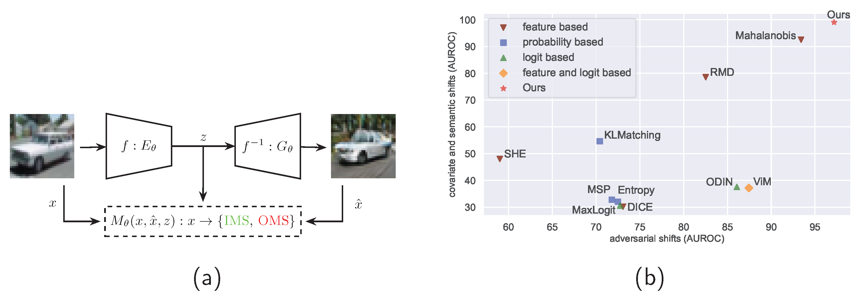
Figure 2.
Figure (a) part illustrates the standard approach of plausibility function in contemporary SW. Figure (b) part of the figure highlights how the monitor M, equivalent to the plausibility function, is being deployed in the computer vision field.
Figure 2.
Figure (a) part illustrates the standard approach of plausibility function in contemporary SW. Figure (b) part of the figure highlights how the monitor M, equivalent to the plausibility function, is being deployed in the computer vision field.
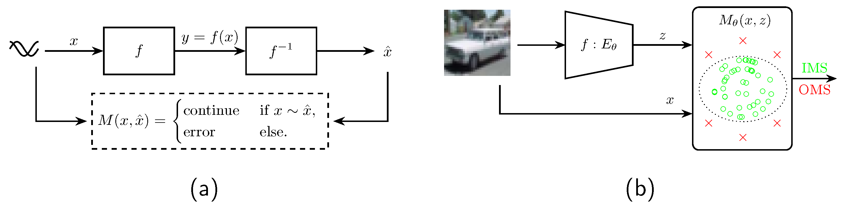
Figure 3.
Our proposed OMS detection pipeline contains the following building blocks: Encoder E, Generator G, Latent Space Wrapper L and OMS monitor O. Each block in this diagram is simplified and can be replaced with more complex or deeper models in order to adapt to a specific domain.
Figure 3.
Our proposed OMS detection pipeline contains the following building blocks: Encoder E, Generator G, Latent Space Wrapper L and OMS monitor O. Each block in this diagram is simplified and can be replaced with more complex or deeper models in order to adapt to a specific domain.
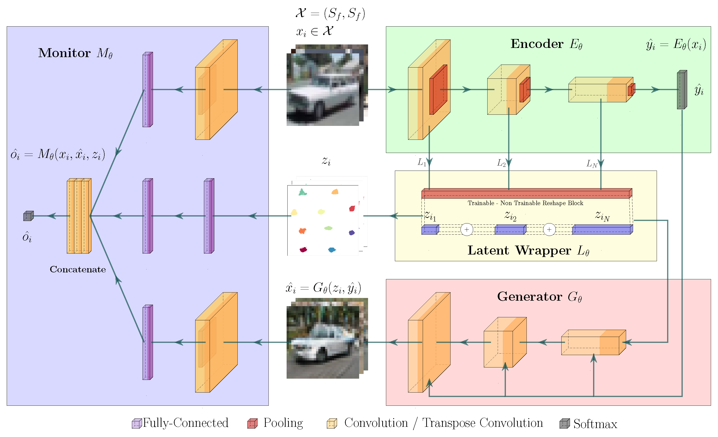
Figure 4.
In the first row, examples of the semantic shifts from Table 1 are visible. We introduce them in the same order as described in Table 1. Additionally, we present the Encoder’s predictions for each image. The second row presents examples of covariate shifts on the original image shown in the first column of the corresponding row. In the final row, the adversarial attacks applied to the original image are visible.
Figure 4.
In the first row, examples of the semantic shifts from Table 1 are visible. We introduce them in the same order as described in Table 1. Additionally, we present the Encoder’s predictions for each image. The second row presents examples of covariate shifts on the original image shown in the first column of the corresponding row. In the final row, the adversarial attacks applied to the original image are visible.
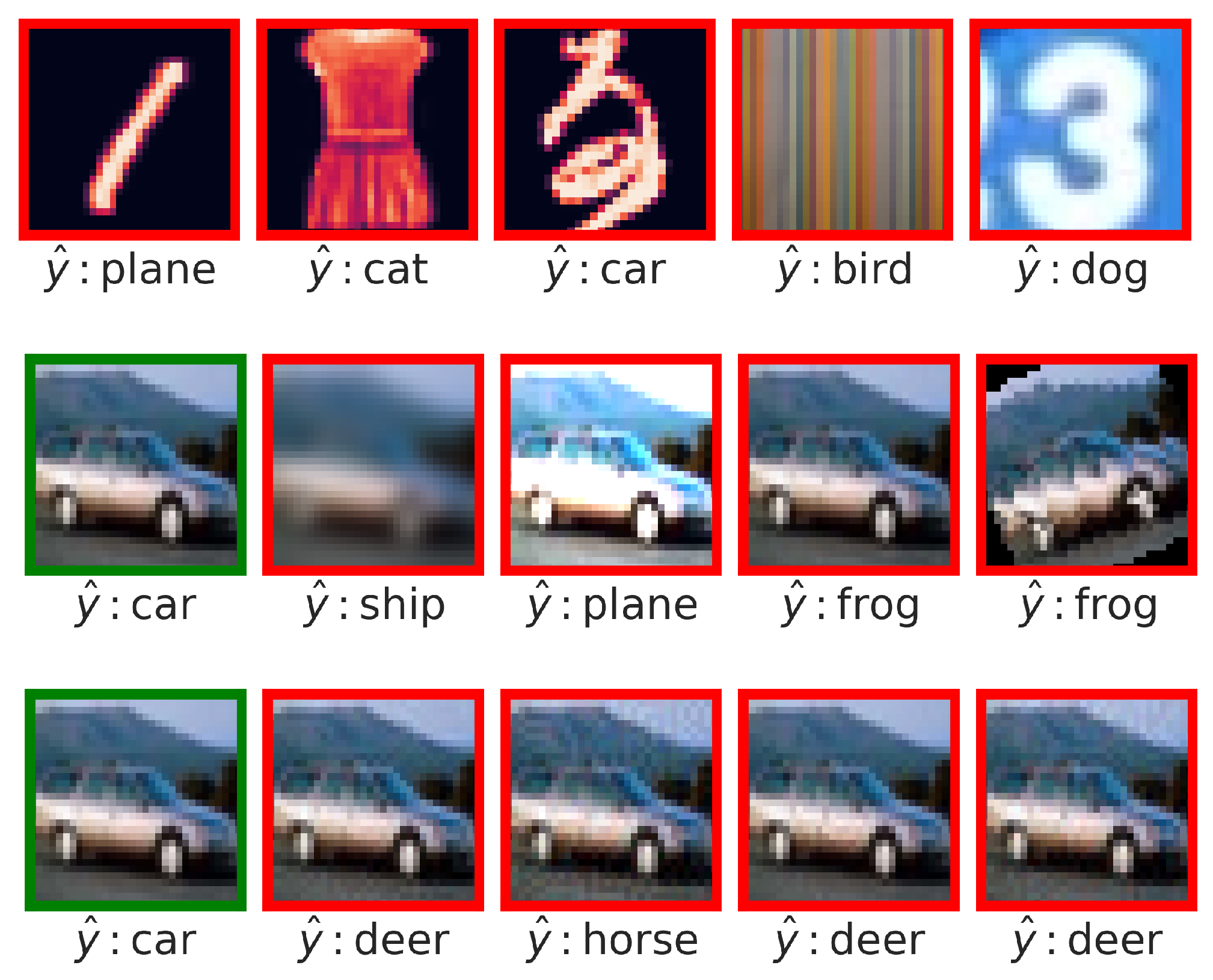
Figure 5.
Figure (a) depicts clustered features from the test set, which contain numerous FPs (orange dots). The presence of FPs causes a sparse and enlarged feature space. The compact feature space in figure (b) was achieved by eliminating the FPs. Nonetheless, some samples remain close to or within the other class cluster, even though the Encoder has classified them correctly. As can be seen in Figure (c), the inner-class compactness subtly changes after applying the Feature Regularizer. The higher distance between the classes "car" and "truck" cluster is even more visible.
Figure 5.
Figure (a) depicts clustered features from the test set, which contain numerous FPs (orange dots). The presence of FPs causes a sparse and enlarged feature space. The compact feature space in figure (b) was achieved by eliminating the FPs. Nonetheless, some samples remain close to or within the other class cluster, even though the Encoder has classified them correctly. As can be seen in Figure (c), the inner-class compactness subtly changes after applying the Feature Regularizer. The higher distance between the classes "car" and "truck" cluster is even more visible.
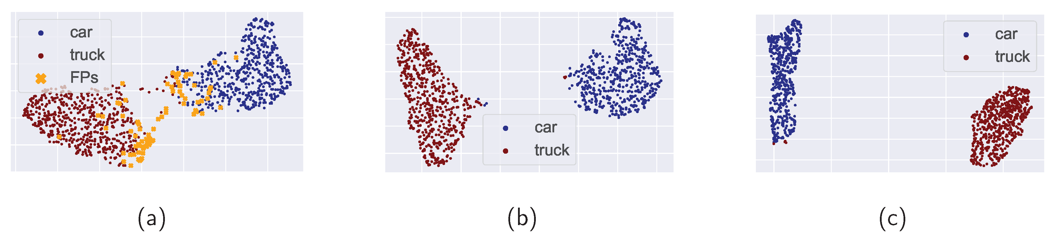
Figure 6.
Figure (a) Variations of latent feature space dimensions only for the bigGAN generator. Best was achieved with the dimension of latent feature space equal to 64. Figure (b) Features form all layers L1+L2+L3+L4 and Latent Space Wrapper with Max-Pooling layers assured the highest in the case of optimal layers’ combination search.
Figure 6.
Figure (a) Variations of latent feature space dimensions only for the bigGAN generator. Best was achieved with the dimension of latent feature space equal to 64. Figure (b) Features form all layers L1+L2+L3+L4 and Latent Space Wrapper with Max-Pooling layers assured the highest in the case of optimal layers’ combination search.
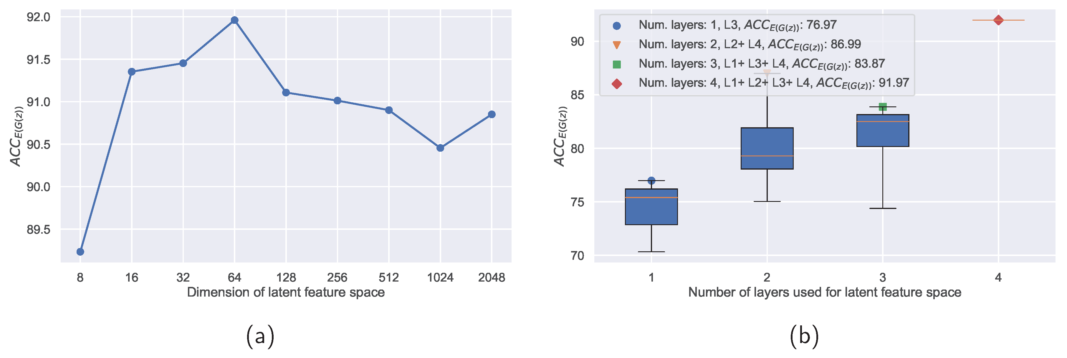
Table 1.
Summary of all methods employed in our experiments in order to construct the OMS datasets.
| IMS | OMS | ||
|---|---|---|---|
| Semantic | Covariate | Adversarial | |
| CIFAR-10 |
MNIST fashionMNIST kMNIST DTD SVHN |
blurring brightness rotation noise |
FGSM PGD DeepFool AutoAttack |
Table 2.
Accuracy of the Encoder - ResNet on different dataset splits. "Dropout" describes a model with a dropout2d layer after each ReLU activation. The best accuracy was achieved by ResNet-34.
Table 2.
Accuracy of the Encoder - ResNet on different dataset splits. "Dropout" describes a model with a dropout2d layer after each ReLU activation. The best accuracy was achieved by ResNet-34.
| ResNet | train. | val. | test | Dropout | FR |
| 18 | 98.94 | 88.64 | 87.01 | 88.69 | 74.06 |
| 34 | 99.48 | 89.88 | 88.18 | 88.99 | 73.51 |
| 50 | 98.89 | 89.19 | 87.73 | 87.76 | 72.12 |
| 101 | 98.35 | 89.10 | 86.71 | 77.72 | 70.09 |
Table 3.
FID, IS and achieved only by the best Generators with ResNet-34. The best model bigGAN model was further used as a Generator in the OMS monitoring pipeline.
Table 3.
FID, IS and achieved only by the best Generators with ResNet-34. The best model bigGAN model was further used as a Generator in the OMS monitoring pipeline.
| model G | ↑IS | ↓FID | Layers Combination | E-regularization | Learnable L | ||
| W-GAN | 5.71 | 38.21 | 70.50 | 64 | L1+L2+L3+L4 | with Dropout | False-Avg Pool |
| bigGAN | 7.92 | 28.04 | 91.96 | 64 | L1+L2+L3+L4 | with Dropout | False-Max Pool |
| CCLDM | 8.01 | 19.87 | 89.89 | 128 | L1+L2+L3+L4 | with Dropout | False-Max Pool |
Table 4.
on the IMS testset for all Encoders and all Generator architectures. The bigGAN architecture has the highest accuracy in combination with ResNet-34. WGAN and CCLDM models didn’t achieve satisfying results and were therefore not taken for further experiments.
Table 4.
on the IMS testset for all Encoders and all Generator architectures. The bigGAN architecture has the highest accuracy in combination with ResNet-34. WGAN and CCLDM models didn’t achieve satisfying results and were therefore not taken for further experiments.
| model E | WGAN | bigGAN | CCLDM |
| 18 | 69.14 | 90.15 | 79.60 |
| 34 | 70.50 | 91.96 | 78.69 |
| 50 | 65.12 | 85.25 | 73.50 |
| 101 | 63.87 | 86.74 | 68.28 |
Table 5.
Influence of different regularization techniques applied to ResNet-34 Encoder on the performance of the bigGAN Generator, , LatentWrapper with maxPool.
Table 5.
Influence of different regularization techniques applied to ResNet-34 Encoder on the performance of the bigGAN Generator, , LatentWrapper with maxPool.
| regularization | ↑IS | ↓FID | |
| no regularization | 6.57 | 30.01 | 90.61 |
| dropout | 7.92 | 28.04 | 91.96 |
| feature regularization | 5.84 | 35.85 | 86.38 |
Table 6.
Presented results of the metrics from the Section 2.3, evaluated on the OMS and IMS test sets. As can be seen in the column "Support", the size of the OMS dataset is approximately bigger than the size of the IMS dataset.
Table 6.
Presented results of the metrics from the Section 2.3, evaluated on the OMS and IMS test sets. As can be seen in the column "Support", the size of the OMS dataset is approximately bigger than the size of the IMS dataset.
| ↑Precision | ↑Recall | ↑F1-score | Support OMS + IMS | |
| 67.42 | 98.76 | 80.14 | 67014 + 4914 |
Table 7.
Our OMS pipeline achieved an overall balanced accuracy of 99.52% on ++. We further evaluated each testset separately, achieving results close to 100%. Notably, the accuracy in recognizing an adversarial attack [2] reached .
Table 7.
Our OMS pipeline achieved an overall balanced accuracy of 99.52% on ++. We further evaluated each testset separately, achieving results close to 100%. Notably, the accuracy in recognizing an adversarial attack [2] reached .
|
Training OMS datasets |
Testset balanced accuracy in [%] | |||
| covariate | adversarial | semantic | ++combined | |
| covariate | 98.95 | 93.04 | 97.99 | 97.93 |
| adversarial | 99.18 | 98.58 | 97.28 | 97.96 |
| semantic | 97.18 | 83.50 | 99.73 | 95.56 |
| combined | 99.21 | 92.25 | 97.76 | 99.52 |
Table 8.
Results of the OMS monitor ablation study. Those results were achieved by setting the corresponding input, or , to zero.
Table 8.
Results of the OMS monitor ablation study. Those results were achieved by setting the corresponding input, or , to zero.
| Deactivated branch | delta acc. [%] to no deactivation |
|---|---|
| Input image x | -25.20 |
| Feature space z | -4.32 |
| Generated image | -3.20 |
| + | -37.36 |
| + | -22.94 |
| + | -32.43 |
| No deactivation | 97.56 |
Table 9.
On the left is an example of a confusion matrix, with terms reflecting the OMS binary classification. The results of our monitoring pipeline are on the right.
Table 9.
On the left is an example of a confusion matrix, with terms reflecting the OMS binary classification. The results of our monitoring pipeline are on the right.
| Total Population | Predicted cls. | ||
| 71928 | Positive (IMS) | Negative (OMS) | |
| True cls. | Positive (IMS) | ↑ TP: IMS as IMS 4701 |
↓ FN: IMS as OMS 213 |
| Negative (OMS) | ↓ FP: OMS as IMS 2289 |
↑ TN: OMS as OMS 64725 |
|
Table 10.
Results on the combined IMS+OMS test set incorporating other SOTA methods.
| Monitor | ↑AUROC | ↑AUPR | ↓FPR95TPR |
| MSP [13] | 61.28 | 95.50 | 100 |
| ODIN [29] | 73.32 | 97.71 | 100 |
| Mahalanobis [26] | 93.74 | 99.52 | 39.50 |
| KLMatching [65] | 66.17 | 95.81 | 83.70 |
| MaxLogit [30] | 61.44 | 95.49 | 100 |
| EnergyBased [24] | 61.30 | 95.42 | 100 |
| Entropy [66] | 61.60 | 95.55 | 100 |
| DICE [67] | 61.60 | 95.50 | 100 |
| RMD [68] | 81.49 | 98.16 | 63.93 |
| ReAct [31] | 62.05 | 95.53 | 99.98 |
| ViM [10] | 74.22 | 97.80 | 99.80 |
| SHE [69] | 56.13 | 95.19 | 100 |
| ours | 99.46 | 93.94 | 3.42 |
Short Biography of Authors
 |
Václav Diviš Autonomous Driving Senior Expert with a proven track record in the automotive industry, namely ARRK Engineering GmbH and ZF Friedrichshafen A.G. Skilled in Automotive SPICE, Functional Safety, Software Development Process, Computer Vision, and Artificial Neural Networks. Currently working on his PhD thesis, focused on Automotive Engineering Technology at the University of West Bohemia, Pilsen, Czech Republic. |
 |
Bastian Spatz Machine Learning Engineer at ARRK Engineering GmbH with a M.Sc. in mathematics from the Technical University of Munich. His main research interests are computer vision, robotics, programming, and scripting. |
 |
Marek Hrúz received a Ph.D. degree in computer science from the Faculty of Applied Sciences, University of West Bohemia in Pilsen, Czech Republic, in 2012. He is currently an Assistant Professor at the Department of Cybernetics, Faculty of Applied Sciences, University of West Bohemia in Pilsen, and a Senior Researcher with the New Technologies for the Information Society. His main research interests are computer vision, machine learning, deep learning, signal processing, and multi-modal signal processing and their application in document analysis, traffic analysis, composite materials welds analysis, and sign language translation. |
Disclaimer/Publisher’s Note: The statements, opinions and data contained in all publications are solely those of the individual author(s) and contributor(s) and not of MDPI and/or the editor(s). MDPI and/or the editor(s) disclaim responsibility for any injury to people or property resulting from any ideas, methods, instructions or products referred to in the content. |
© 2024 by the authors. Licensee MDPI, Basel, Switzerland. This article is an open access article distributed under the terms and conditions of the Creative Commons Attribution (CC BY) license (http://creativecommons.org/licenses/by/4.0/).
Copyright: This open access article is published under a Creative Commons CC BY 4.0 license, which permit the free download, distribution, and reuse, provided that the author and preprint are cited in any reuse.


