
Submitted:
22 August 2024
Posted:
27 August 2024
You are already at the latest version
Abstract
The Normalized Differential Spectral Attenuation (NDSA) technique was proposed years ago as an active method for measuring Integrated Water Vapor (IWV) along a Ku/K-band radio link immersed (totally or partially) in the troposphere. The approach is of the active kind, as it relies on the transmission of a couple of sinusoidal signals, whose power is measured at the receiver, thus providing the differential attenuation measurements from which IWV estimates can be in turn derived. In 2018, a prototype instrument providing such differential attenuation measurements was completed and set up for a first measurement campaign aimed at demonstrating the NDSA method. By the end of June 2022, the instrument was profoundly modified and upgraded so that a second measurement campaign could be carried out from August 1 to November 30, 2022. The transmitter was placed on the top of Monte Gomito (44.1277°lat, 10.6434°lon, 1892 m a.s.l.) and the receiver on the roof of the Department of Information Engineering of the University of Florence (43.7985°lat, 11.2528°lon, 50 m a.s.l.). The resulting radio link length was 61.15 km. Four ground weather stations of the regional weather service were selected among those available. In this paper, we describe the upgraded instrument and present the outcomes of the new measurement campaign, whose purpose was mainly to compare the IWV estimates provided by the instrument with the ground sensors measurements of air temperature, air humidity, barometric pressure, and rainfall.
Keywords:
microwaves
; water vapor
; troposphere
; differential attenuation
1. Introduction
The so-called Normalized Differential Spectral Attenuation (NDSA) method has been proposed as a new active remote sensing approach to provide estimates of the Integrated Water Vapor (IWV) - defined as the total mass of the Water Vapor (WV) - along tropospheric paths. This is achieved through attenuation measurements at microwave frequencies, specifically in the Ku/K-bands. As detailed in [1,2], two sinusoidal signals with frequencies that are very close to each other with respect to their average value are transmitted and their receive power measured. Based on a parameter called ’spectral sensitivity’, which is essentially a normalized form of the differential attenuation between the transmitter (TX) and the receiver (RX), it is possible to estimate the IWV along the TX-RX link. This was theoretically demonstrated based on the millimeter-wave propagation model (MPM) described in [3], on extensive analyses of radiosonde data [2] and Numerical Weather Prediction (NWP) reanalysis model data [4]. The reason for using values of in the Ku/K-bands is their closeness to the WV absorption line at 22.235 GHz. There, the slope of the absorption spectrum depends mainly on the WV content along the radio link, as the contributions of the other atmospheric components are practically constant with frequency.
The NDSA method can be usefully exploited for providing more in depth analysis of the WV content in the lower troposphere. Pursuing this objective with systematic measurements on a global scale would be of great importance to achieve several objectives, since the amount of water available for precipitation in any form depends on the global and local dynamics of WV. A better knowledge of such dynamics would improve NWP models on short time scales. In fact, the latent heat exchange processes caused by WV phase changes influence the atmospheric thermal profiles. As a consequence, the atmospheric transport processes are driven by WV, so that measuring WV concentration and its variations in space and time is of paramount importance in meteorology and climatology [5,6,7,8], but how to achieve such an objective with the appropriate resolution and sensitivity is still an open question [9,10,11].
Theoretical studies conducted for the European Space Agency (ESA) [12,13,14] have shown that, exploiting the IWV estimates gathered through the NDSA method applied to the radio paths connecting pairs of TX and RX mounted on Low Earth Orbiting (LEO) satellites, it is possible to provide global estimates of WV. Attenuation measurements are performed in limb mode, while different WV retrieval methods can be implemented in the case that the LEO satellites orbit in opposite directions in the orbital plane [2,15], or along the same direction [16,17].
The first practical implementation of the NDSA measurements was possible thanks to the SWAMM (Sounding Water vapour by Attenuation Microwave Measurements) project, funded by the Tuscan regional administration. During SWAMM, the first NDSA instrument prototype - referred to as SWAMM-1 hereafter - was built as a low-cost instrument capable of providing ground-to-ground spectral sensitivity measurements at 19 GHz. The reasons for selecting this central frequency and 400 MHz as the spectral separation of the two transmit frequencies (= 18.8 GHz and = 19.2 GHz, implying a fractional bandwidth of 2%) are highlighted in [18]. A measurement campaign with SWAMM-1 was carried out in Central Italy with a ground-based TX-RX link of about 60 km length. Its results have been recently published [19]. The two independent units of SWAMM-1 were the TX, which transmitted (non-simultaneously) two tones at and , and the RX, which collected and recorded the received powers. A software-designed module was implemented for data acquisition and processing, and for the delivery of the final product (i.e., the two calibrated single-tone powers).
By the end of June 2022, a significant improvement of the instrument prototype was completed, so that a new measurement campaign could be carried out from August 1 to November 30, 2022. The upgraded prototype is referred to as SWAMM-2 in the following. The campaign was part of the activities of the SATCROSS (co-rotating satellites for the tropospheric water vapor estimation) project funded by the Italian Space Agency, aimed at assessing the feasibility of the NDSA technique. In this paper, we summarize the SWAMM-1 prototype updates that led to SWAMM-2, describe the 2022 measurement campaign and analyze the NDSA products from the SWAMM-2 instrument by comparing them with the ground point data of air temperature, air humidity, barometric pressure, and rainfall.
This article is a revised and expanded version of a paper entitled "Integrated water vapor estimation through microwave propagation measurements: second experiment on a ground-to-ground radio link", which was presented at the IGARSS 2023 conference held in Pasadena (USA), in July 2023 (see [20]). The paper is structured as follows. In Section 2, the features of the improved instrument SWAMM-2 are described in detail. In Section 3, we present the TX-RX set up of the new measurement campaign, while in Section 4 we show and critically analyze the results. In Section 5, the conclusions are drawn.
2. The NDSA Approach and the SWAMM-2 Prototype
In this Section, we first provide a brief overview of the NDSA approach to estimate the IWV along a microwave link. Then, we describe in detail the upgraded instrument SWAMM-2 for NDSA measurements.
2.1. Spectral Sensitivity and IWV
As indicated in [19] and papers cited therein, the NDSA technique requires two sinusoidal signals with different frequencies and () to be transmitted. In fact, the technique is based on the measurement of the spectral sensitivity
where is the reference central frequency while and are the atmospheric attenuations undergone by the two tones along the radio path. Assuming that the two sinusoidal signals are radiated with different transmit powers and , and denoting with and the corresponding powers at the receiver end, Equation (1) becomes
The NDSA estimate of IWV is then derived from as follows
In general, the coefficients and depend on , on the spectral separation and on the measurement geometry. For satellites applications (limb measurements between TX and RX on board two different satellites), the values of and are listed in [4], while for ground-based applications they are reported in [18]. In both cases, the coefficients were derived through simulations based on propagation models and atmospheric databases. In this work, and are derived based on a regression applied to real measurements.
2.2. The SWAMM-2 Instrument for Spectral Sensitivity Measurements
As mentioned in the Introduction, the SWAMM-2 instrument operates with a spectral separation of 400 MHz, being = 18.8 GHz and = 19.2 GHz. Being = 19 GHz, the spectral sensitivity measured is indicated as in the following.
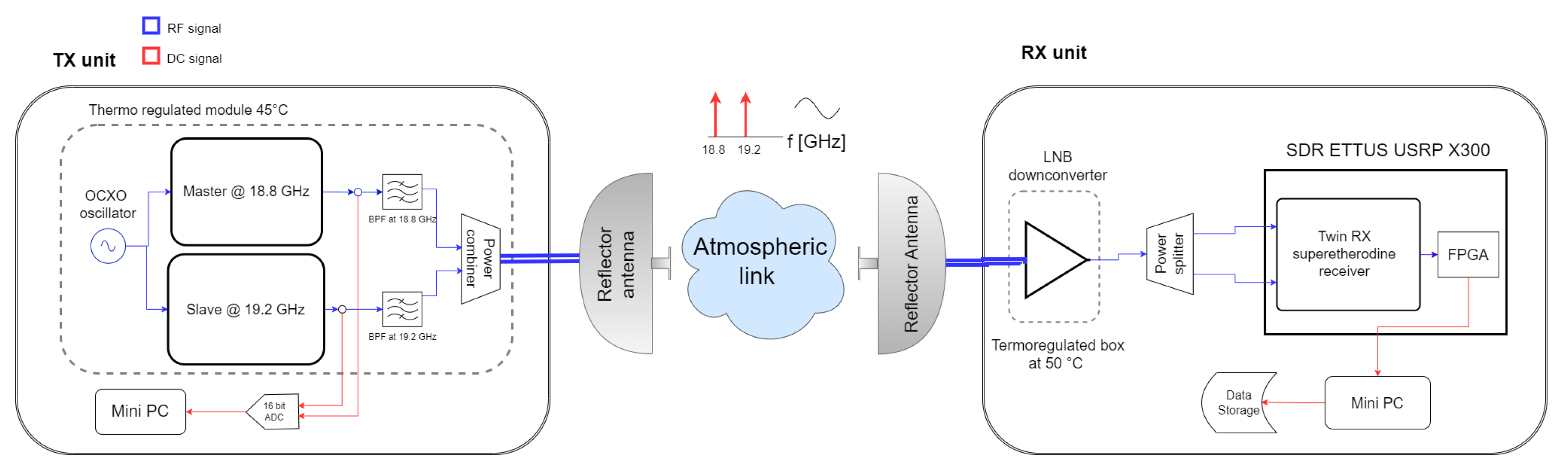
One of the limitations of the SWAMM-1 prototype was the impossibility of carrying out simultaneous power measurements, as the two sinusoidal signals at and were transmitted alternately, with a duty cycle of 0.5 seconds, by using a commercial RF synthesizer. The new TX unit in SWAMM-2, shown in Figure 5, is designed to simultaneously transmit two sinusoidal tones with a constant power. This allows and to be measured in the same time intervals; in this manner, fluctuations due to tropospheric scintillation are recorded correctly and reduced, since the additional fluctuations generated by the temporal misalignment of the two received signals are removed.
Because of the high level of stability needed to perform accurate measurement of , the TX architecture consists of two modules based on a Phase Locked Loop (PLL) which operates in master-slave mode and sharing the same clock reference. The internal reference oscillator is an Oven Controlled Crystal Oscillator (OCXO) working at 100 MHz (Abracon AOCJY). The MASTER module generates the 18.8 GHz sinusoidal signal, while the SLAVE one generates that at 19.2 GHz. The two modules are in thermal contact to ensure the same temperature variation, so as to minimize its impact on the differential power measurement. To limit the thermal excursion that can impact the transmit power level, a thermo-regulated box has been designed to work in a range of ± 2.0°C from the setpoint of 45°C. Each generated tone is filtered by a narrow-band filter with a 200 MHz bandwidth and then combined in a single WR42 flexible waveguide, which is connected to the antenna.
An additional enhancement to the TX unit is the ability to monitor the powers and that are necessary for computing and to compensate the TX power drifts during the entire campaign. To this end, a portion of the transmitted power is extracted from both the MASTER and SLAVE modules using a directional coupler, and measured by an internal square-law detector. The TX power output has been measured at the TX output flange by means of the calibrated power meter (PM) Anritsu MA24340A. The nominal power output is 18 dBm. The output voltages are digitized by a 16 bit Analog to Digital Converter (ADC) and sent to a Raspberry-Pi.
The new RX unit of SWAMM-2 is based on a Software Defined Radio (SDR) platform. The first stage of the receiver is a Low-Noise Block (LNB) downconverter, directly connected to the receiving antenna through a WR42 waveguide. The LNB performs a low-noise amplification of about 55 dB and converts the frequencies of the received tones from 18.8 and 19.2 GHz down to intermediate frequencies () of 1.55 and 1.95 GHz, respectively. The IF signal is divided into two separate paths using a resistive power divider, allowing simultaneous processing by the USRP (Ettus X300). The latter is equipped with a Twin RX superetherodyne receiver, which operates the last frequency conversion before being sampled by the FPGA’s ADC at a rate of 210 MS/s with a 14-bit resolution. The digital data stream is decimated to reach the final sampling rate of 250 kS/s, then digitally filtered by a Finite Impulse Response (FIR) low pass filter with a 40 kHz bandwidth. The output data stream is buffered and transmitted to a mini Personal Computer (PC), which is integrated in the RX unit. The mini PC handles the final processing of the output data stream from the SDR, comprising 12.5 kS for every 50 ms of acquisition.
Two different output power estimates are generated for each receive channel, defined as follows: i) the average power , obtained by squaring the RMS (root mean square) voltage of the output signal; ii) , representing the highest peak of the power spectrum, estimated through Fast Fourier Transform (FFT). Ideally, only one spectral peak should be present per receive channel. The presence of additional peaks is the effect of intermodulation processes due to the device’s imperfect linearity. Unlike , the metric helps to get rid of these unwanted contributions.
The entire system has been accurately configured to operate across a wide range of attenuation levels, as required for the ground-to-ground campaign. The lowest attenuation levels are expected in clear air, and the highest in the presence of rainfall.
Special attention has been given to characterizing the SDR board’s capability to estimate the received power in the presence of disturbances. Besides thermal noise, these disturbances include spurs resulting from the SDR board’s imperfect linearity, affecting both the and power estimates. For improved characterization, we utilized the spurious free dynamic range (SFDR) parameter, which is the ratio (in dB) between the fundamental tone and the highest spur in the estimated power spectrum. Using a calibrated signal generator, we generated tones at the two aforementioned IF frequencies (1.55 GHz and 1.95 GHz) with power levels ranging from -80 to -20 dBm in 10 dBm increments, which were then input to the receiver. The SDR noise floor was determined by turning off the input source.
Figure 1 shows the SFDR versus the output of the processing chain for both and as a function of the power measured by the receiver (in dBm). Note that and take the same values as long as SFDR >20 dB (corresponding to -70 dBFS). At lower SFDR levels, tends to saturate sooner than . This behaviour occurs because the computation of involves the entire 40 kHz bandwidth, thereby including the effect of the spectral spurs generated by the SDR’s nonlinearities. In contrast, the computation of focuses solely on the primary spectral component of interest, which remains unaffected by spurs as long as it is above the highest spur peak level, i.e., above -90 dBm. For this reason, we used for measurements, and retained only for cross-checking. It is important to note that, in the absence of rainfall, the expected output range is between -45 and -25 dBm, where the SFDR consistently remains above 40 dB for both the 1.55 GHz and 1.95 GHz IF channels.
The calibration of the TX-RX system involved the elimination of the contribution to the overall differential attenuation that is systematically introduced by the instrument [19]. For this purpose, TX and RX were connected via a series of variable WR42 waveguide attenuators, as shown in Figure 2, with both the TX and the RX maintained at room temperature. The range of variation of the total attenuation was chosen to match that expected during the campaign; this means from a minimum level corresponding to the free space path loss (153.7 dB for the 61 km length link in clear air) to a maximum level of 212.7 dB, which reduces the signal power to the average RX noise power level. The total path attenuation, obtained by dropping the contribution of the antenna gains, ranges from 74 to 153 dB. In fact, the TX and RX antennas are commercial parabolic reflectors with a combined gain of 59.7 dBi, operating at vertical polarization.
Figure 3a displays the uncalibrated power at the RX output versus the calibrated power at the RX input, for both receive channels, evidencing the high linearity of both curves in the whole operational range. The calibration process has included the overall differential antenna gain contribution provided by the manufacturer, i.e. dB. Figure 3b shows the differential attenuation of the TX-RX chain versus the path loss expected during the campaign, both before and after the calibration.
Moreover, since both the TX and the RX contain temperature-sensitive devices, the calibration curve depends on temperature. Consequently, both units have been independently characterized thermally. The TX was placed inside a thermal chamber with a controlled temperature (accuracy of ± 0.01 °C), ranging from 10°C to 50°C in 5°C increments. The transmitted power of each tone was measured by a PM, located outside the chamber at room temperature and connected to the transmitter via a flexible WR42 waveguide. At the same time, the output voltages of the internal square law detector were calibrated using the PM as a reference. The resulting thermal curves relative to and were used to correct the power measured by the internal detector during the test and subsequent experimental campaign. The residual error is defined as the difference between the thermally corrected TX differential power output, expressed in dB as , and the reference PM level. Such error is shown in Figure 4a versus the internal TX temperature. has been characterized in the thermal range from 15°C to 50°C, when the TX was not thermo-regulated. During the campaign, the thermo-regulation was applied, maintaining the temperature within ± 2°C around the set-point of 45°C (as highlighted in Figure 4a), resulting in being limited to ± 0.03 dB. Thus, the estimated uncertainty of the TX power due to temperature variations is 0.03 dB.
A similar thermal characterization was performed for the RX. In this case, the setup depicted in Figure 2 was used, but with the TX at room temperature and the RX was placed inside the thermal chamber. The same set of WR42 waveguide attenuators used for calibration were inserted between the TX and the RX. The RX power gain, defined as the difference between the power measured at the TX output (temperature-dependent) and the input power to the RX (at room temperature), was characterized against the temperature of the climatic chamber. The resulting curve has been then used for thermal correction.
The differential gain of the entire RX chain expressed in dB as , is shown in Figure 4b before and after temperature correction. The obtained residual leads to an estimate of RX thermal uncertainty of ± 0.04 dB from 23 to 45 °C.
A summary of the instrumental uncertainties is given in Table 1. Note that total instrumental uncertainty is ± 0.19 dB on the differential attenuation, which reduces to ± 0.12 dB when considering only high SNR levels.
3. Measurement Setup and Campaign
The SWAMM-2 instrument, whose functional diagram is shown in Figure 5, was utilized for a new measurement campaign in Tuscany, Italy, from July to November, 2022. The TX was installed at the summit of Monte Gomito (44.1277° lat., 10.6434° lon., 1892 m altitude) and the RX on the roof of the Department of Information Engineering at the University of Florence (43.7985° lat., 11.2528° lon., 50 m altitude). The radio link spanned a distance of 61.15 km. Additionally, a webcam was set up at the TX site pointing towards the RX site, to provide continuous qualitative information on atmospheric conditions (i.e., clear sky/cloud/rainfall/fog) throughout the day. In order to perform a comparative analysis with respect to the measurements provided by the SWAMM-2 instrument, data collected by the network of weather stations of the “Regional hydrological Service of Tuscany” were used. The network covers the whole regional territory and consists of measurement sites equipped with a complete set of weather sensors (pressure, temperature, wind, humidity and rainfall). There are more than 600 of these sites over Tuscany, providing measurements every 15 minutes. Data are available in nearly real time (a few minutes time lag) through a dedicated communication infrastructure. Among these weather stations, the two closest to the RX site and the two closest to the TX site were selected. Figure 6 shows the geographical position of the radio link and of the four stations considered, whose IDs and coordinates are reported in Table 2, while Figure 7 displays the webcam view directed towards the receiver. The atmospheric parameters used in our analysis are: 1) pressure, temperature and relative humidity provided by the weather stations, so as to compute the absolute humidity at each site; 2) the 15-minutes cumulative rainfall to monitor precipitation, which may cause strong attenuation at the frequencies used, in some cases even leading to signal extinction.
Figure 5.
Functional diagram of the NDSA measurement system.
4. Experimental Results
The absolute humidity values computed at the four weather stations shown in Figure 6 have been employed to provide independent estimates of the IWV along the TX-RX link according to the following procedure. First, and were computed as the averages of the WV concentration measurements from the two stations close to the TX and to the RX, respectively; then, the IWV along the radio link was estimated assuming that the WV content varied linearly between the two values and , i.e.
where L denotes the length of the radio link. The SWAMM-2 instrument’s estimate of IWV is derived using the linear relation given in Equation (3), with 19 GHz, =34 · and =-21 . These values were obtained by applying a linear regression procedure to the measured values of and . From this linear relation and the results of Table 1, the overall IWV uncertainties can be derived: the uncertainty in the IWV estimate due to the instrument is 12.67 across the entire signal range, from the lowest to the highest signal-to-noise ratios. In clear air conditions, this uncertainty decreases to 8.27 .
Figure 8, which shows the complete sequence of data collected from 21 July to 21 November 2022, provides an overall view of the parameters measured during the campaign. Specifically, the plots labeled “18.8 GHz Ch” and “19.2 GHz Ch” show the 10 s average power of the signals received on the two NDSA channels. As discussed in Section 2 and shown in Figure 1, the spurious level of the power is reached at around -90 dBFS. A margin of 20 dBFS has been introduced, therefore data below -70 dBFS have been discarded. The longer periods of time with no SWAMM-2 signal in Figure 8 correspond to the intervals when the instrument was switched off due to supply interruption.
The curves show the IWV estimates obtained by inserting the SWAMM-2 measurements of into Equation (3). The RX Temp curves show the mean temperature of the RX1-RX2 pair, available every 15 minutes; analogously, the TX Temp curves show the mean temperatures of the TX1-TX2 pair, also available every 15 minutes. It is worth noting that the cyclical variations of RX Temp and TX Temp provide a clear daily time reference. In fact, the highest values occur during the warmest part of the day (3-4 PM local time), while the lowest values coincide with sunrise.
The curves report the moving average over one hour of the data, with 15 minutes time step. The plot marked as RAIN is a sequence of binary levels with a time step of 15 minutes indicating the presence (-10 level) or the absence (0 level) of rainfall in at least one of the four weather stations in the preceding 15 minutes.
The signal drops on both receive channels are caused by precipitation along the TX-RX radio link. This evidenced in better detail by Figure 9, reporting the 24 hours data of August 7, 2022 and the webcam image taken at 11.20 AM, clearly showing the presence of rainfall. In fact, a typical short summer storm occurred between 11.00 and 14.30 in the measurement area. Analogously, Figure 10 shows the 24 hours data of July 28, 2022, when a thunderstorm occurred between 13.00 and 15.00 in the measurement area. In this second case, the total attenuation was quite smaller, indicating a lower level of average rainfall rate along the link. It is important to note that in both cases there is no impact on the estimates, as the two receive powers undergo the same attenuation thanks to the proximity of the two frequencies used. Therefore, as long as the two received signals keep above -70 dBFS, both IWV and the average rainfall rate along the radio path can be estimated.
The presence of non precipitating water (i.e., clouds, fog, haze) along the link may cause a bias in the IWV estimates that is proportional to the liquid water mass content (see [2], referring to a satellite-to-satellite link). This condition was observed several times during the campaign. For instance, Figure 11 reports the data of 21 October 2022, a day characterized by a shift from clear weather conditions to unsettled ones. Around 9:00 in the morning, the sky began to cloud over, and by early afternoon, the TX site was immersed in fog until 6:00 PM, when it started raining and continued to do so for the next three days. Note that the presence of clouds and fogs did not cause a measurable decrease of the received powers. The reason is that the radio link length of 61.5 km is insufficient to encompass a significant amount of liquid water that could bias the differential power measurements.
Observing Figure 8, note that there are periods during which the received powers and fluctuate significantly. In some cases, the amplitude of the fluctuations are such, that takes negative values. One of the most significant periods featuring strong fluctuations is that reported in Figure 12. It refers to data collected in the week from 31 July to 6 August, when stable warm atmospheric conditions (high pressure, sunshine, clear sky) were recorded. As can be noted by observing the two signal powers, such atmospheric conditions favor the occurrence of fluctuations from the central hours of the night, as temperature starts decreasing, until the early hours of the morning. Instead, during the warmest hours of the day, the amplitude of such fluctuations is significantly reduced. This behaviour was typically observed in the absence of unsettled weather conditions: see for instance Figure 11 and note that the amplitude fluctuations are reduced as soon as the weather conditions shift from clear to unsettled. In general, the cause of the fluctuations is atmospheric turbulence, which is generated by the spatial irregularity of the refraction index [21]. This generates the multipath effects that are at the basis of the so called scintillation phenomenon, namely amplitude fluctuations whose intensity is greater, the greater the turbulence.
For an appropriate comparison between and , it is important to recognize the significant spatial variability of the atmospheric parameters that determine absolute humidity. In this regard, consider the scatter plots of Figure 13, comparing temperature and relative humidity of the pairs TX1-TX2, and Figure 14, comparing temperature and relative humidity of the pair RX1-RX2. The correlation coefficients between the temperature and relative humidity measurements at the two stations close to the RX site are 0.99 and 0.72, respectively. For what concerns the two stations close to the TX site, the correlation coefficients are 0.94 and 0.52, respectively. This implies that within a few km distance, remarkable variations of absolute humidity are normally encountered. As a consequence, the estimate of the integral content of WV is provided by two estimates of absolute humidity made at the ends of the link ( and ), which are intrinsically subject to high quantitative uncertainty. Therefore, a quantitative comparison between and should be approached with extreme caution. From a qualitative standpoint, it can be noted that even though and often exhibit the same trend (see for instance Figure 15 and Figure 16), this is not always the case (see Figure 12). While we cannot state that there is a clear correlation between and in terms of daily, weekly and monthly trends, we point out that the daily variations of match very well those of the temperatures at the TX and RX. This suggests that is a more reliable estimate of the WV content along the radio link than , which is affected both by the aforementioned uncertainties at the ends and by the deviations from the assumption of linear variation made to derive Equation (4).
The picture that illustrates the overall statistical relation between the measurements by the SWAMM-2 instrument and the IWV estimates derived using the meteorological stations is shown in the scatter plots of Figure 17, which shows the spectral sensitivity measurements averaged over 1 hour vs . Specifically, the red markers refer to the whole campaign data, while the green ones refer only to data acquired in those meteorological conditions that do not affect IWV measurements. Such conditions are: a) absence of rainfall over all the four weather stations; and b) relative humidity lower than 100% over all the four weather stations. The correlation coefficients of the red and green scatter plot are 0.68 and 0.71, respectively, which demonstrates that a decent statistical link between what was observed by the SWAMM-2 instrument and by the 4 weather stations.
5. Conclusions
An enhanced version of an instrument for performing spectral sensitivity measurements at 19 GHz and estimating integrated water wapor along a radio link through the NDSA approach has been developed and utilized in a three-month measurement campaign.
Besides interruptions not caused by malfunctioning, the instrument contibuously provided NDSA measurements in any kind of atmospheric condition occurred in that period. Notably, even in the presence of rainfall, clouds and fog, the differential attenuation (from which the spectral sensitivity and the IWV estimates are derived) showed no deviation from its behaviour in clear air. This is a positive outcome because it demonstrates for instance that, despite the significant absolute attenuation caused by rainfall, IWV measurements can still be performed as long as the transmission power is adequately high relative to the link length. The campaign evidenced a clear correlation between the temporal variations of the IWV estimates provided by the instrument and the temperatures at the ends of the radio link. These were recorded by the four ground weather stations which also provided the relative humidity measurements near the link ends. In this regard, it is noteworthy that the analysis of the temperature and relative humidity data provided by such weather stations evidenced a rather low level of correlation of absolute humidity measurements that are taken a few km apart near either the TX or RX site, highlighting a high spatial variability of the parameter of interest. A similar level of correlation was observed when comparing the NDSA prototype’s measurements and the IWV estimates derived from the average weather stations’ measurements. This discrepancy is likely caused by the substantial spatial variability in temperature and relative humidity, which makes it challenging to accurately assess the IWV estimates provided by the NDSA instrument.
Author Contributions
Conceptualization, L.F. and F.C.; methodology, L.F.,F.C., U.C., S.d.B., M.G. and F.M. ; software, F.C. and M.G.; formal analysis, L.F., F.C. and G.M.; resources, U.C., S.dB., and G.M.; data curation, F.C., M.G. and F.M.; investigation, F.C., M.G. and F.M.; writing—original draft preparation, F.C.and F.M.; writing—review and editing, L.F. and F.C.; supervision, L.F.; project administration, L.F.; funding acquisition, L.F. All authors have read and agreed to the published version of the manuscript.
Funding
The research activities described in this paper were carried out with contribution of the Next Generation EU funds within the National Recovery and Resilience Plan (PNRR), Mission 4 - Education and Research, Component C2 - From Research to Business (M4C2), Investment Line 1.1 - Fund for the National research program and projects of significant national interest (PRIN), Project 2022JJJYTE – “Measuring tropospheric water vapour through the Normalized Differential Spectral Attenuation (NDSA) technique”.
Abbreviations
The following abbreviations are used in this manuscript:
| ADC | Analog to Digital Converter |
| ESA | European Space Agency |
| FIR | Finite Impulse Response |
| FFT | Fast Fourier Transform |
| FPGA | Field Programmable Gate Array |
| LNB | Low Noise Block |
| IF | Intermediate Frequency |
| LEO | Low Earth Orbiting |
| MPM | Millimeter Wave Propagation Model |
| NDSA | Normalized Differential Spectral Attenuation |
| NWP | Numerical Weather Prediction |
| OCXO | Oven Controlled Crystal Oscillator |
| PC | Personal Computer |
| PLL | Phase Locked Loop |
| PM | Power Meter |
| RX | Receiver (or receiving) |
| RF | Radio Frequency |
| RMS | Root Mean Square |
| SFDR | Spurious Free Dynamic Range |
| TX | Transmitter (or transmitting) |
| SDR | Software Defined Radio |
| SWAMM | Sounding Water Vapor by Attenuation Microwave Measurements |
| WV | Water Vapor |
| IWV | Integrated Water Vapor |
References
- Cuccoli, F.; Facheris, L. Normalized differential spectral attenuation (NDSA): a novel approach to estimate atmospheric water vapor along a LEO-LEO satellite link in the Ku/K bands. IEEE Transactions on Geoscience and Remote Sensing 2006, 44, 1493–1503. [Google Scholar] [CrossRef]
- Facheris, L.; Cuccoli, F.; Argenti, F. Normalized differential spectral attenuation (NDSA) measurements between two LEO satellites: performance and analysis in the Ku/K bands. IEEE Transactions on Geoscience and Remote Sensing 2008, 46, 2345–2356. [Google Scholar] [CrossRef]
- Liebe, H.; Hufford, G.; Cotton, M. Propagation Modeling of Moist Air And Suspended Water/Ice Particles at Frequencies below 1000 GHz; AGARD 52nd Specialists Meeting of the Electromagnetic Wave Propagation Panel on “Atmospheric Propagation Effects through Natural and Man-Made Obscurants for Visible to MM-Wave Radiation”,, 1993.
- Facheris, L.; Cuccoli, F. Global ECMWF analysis data for estimating the water vapor content between two LEO satellites through NDSA measurements. IEEE Transactions on Geoscience and Remote Sensing 2018, 56, 1546–1554. [Google Scholar] [CrossRef]
- Kaufmann, Y.; Gao, B. Remote sensing of water vapor in the near IR from EOS/MODIS. IEEE Transactions on Geoscience and Remote Sensing 1992, 30, 871–884. [Google Scholar] [CrossRef]
- Li, X.; Dick, G.; Lu, C.; Ge, M.; Nilsson, T.; Ning, T.; Wickert, J.; Schuh, H. Multi-GNSS meteorology: real-time retrieving of atmospheric water Vapor from BeiDou, Galileo, GLONASS, and GPS observations. IEEE Transactions on Geoscience and Remote Sensing 2015, 53, 6385–6393. [Google Scholar] [CrossRef]
- Negusini, M.; Petkov, B.H. and Sarti, P.; Tomasi, C. Ground-based water vapor retrieval in Antarctica: an assessment. IEEE Transactions on Geoscience and Remote Sensing 2016, 54, 2935–2948. [Google Scholar] [CrossRef]
- Tang, A. and Kim, Y.; Xu, Y.and Virbila, G.; Reck T.and Chang, M.C.F. Evaluation of 28 nm CMOS receivers at 183 GHz for space-borne atmospheric remote sensing. IEEE Microwave and Wireless Components Letters 2017, 27, 100–102. [Google Scholar] [CrossRef]
- Weaver, D.; Strong, K.; Schneider, M.; Rowe, P.; Sioris, C.; Walker, K.A.; Mariani, Z.; Uttal, T.; McElroy, C.T.; Vömel, H.; Spassiani, A.; Drummond, J. Intercomparison of atmospheric water vapour measurements at a Canadian High Arctic site. Atmos. Meas. Tech. 2017, 10, 2851–2880. [Google Scholar] [CrossRef]
- Borger, C.; Schneider, M.; Ertl, B.; Hase, F.; García, O.E.; Sommer, M.; Höpfner, M.; Tjemkes, S.A.; Calbet, X. Evaluation of MUSICA MetOp/IASI tropospheric water vapour profiles by theoretical error assessments and comparisons to GRUAN Vaisala RS92 measurements. Atmos. Meas. Tech. Discuss. 2017, 11, 4981–5006. [Google Scholar] [CrossRef]
- Stevens, B.; Bony, S. What Are Climate Models Missing? 2013. 340, 1053–1054.
- Facheris, L.; Cuccoli, F.; others. Alternative Measurement Techniques for LEO-LEO Radio Occultation. Final Report ESA-ESTEC Study Contract No. 17831/03/NL/FF, 2004.
- Kirchengast, G.; Facheris, L.; others. Study of the Performance Envelope of Active Limb Sounding of Planetary Atmospheres. Final Report ESA-ESTEC Study Contract 21507/08/NL/HE, 2010.
- Facheris, L.; others. Analysis of normalised differential spectral attenuation (NDSA) technique for inter-satellite atmospheric profiling,” Final Report of the ESA–ESTEC Study Contract No. 4000104831, 2013.
- Facheris, L.; Cuccoli, F.; Martini, E. Tropospheric IWV profiles estimation through multifrequency signal attenuation measurements between two counter-rotating LEO satellites: performance analysis. Proc. SPIE 8890, Remote Sensing of Clouds and the Atmosphere XVIII; and Optics in Atmospheric Propagation and Adaptive Systems XVI 2013, 8890. [Google Scholar] [CrossRef]
- Lapini, A.; Cuccoli, F.; Argenti, F.; Facheris, L. The Normalized Differential Spectral Sensitivity Approach Applied to the Retrieval of Tropospheric Water Vapor Fields Using a Constellation of Corotating LEO Satellites. IEEE Transactions on Geoscience and Remote Sensing 2016, 54, 135–152. [Google Scholar] [CrossRef]
- Mazzinghi, A.; Cuccoli, F.; Argenti, F.; Feta, A.; Facheris, L. Tomographic Inversion Methods for Retrieving the Tropospheric Water Vapor Content Based on the NDSA Measurement Approach. Remote Sensing 2022, 14. [Google Scholar] [CrossRef]
- Di Natale, G.; Del Bianco, S.; Cortesi, U.; Gai, M.; Macelloni, G.; Montomoli, F.; Rovai, L.; Melani, S.; Ortolani, A.; Antonini, A.; Cuccoli, F.; Facheris, L.; Toccafondi, A. Implementation and Validation of a Retrieval Algorithm for Profiling of Water Vapor From Differential Attenuation Measurements at Microwaves. IEEE Transactions on Geoscience and Remote Sensing 2019, 57, 5939–5948. [Google Scholar] [CrossRef]
- Montomoli, F.; Macelloni, G.; Facheris, L.; Cuccoli, F.; Del Bianco, S.; Gai, M.; Cortesi, U.; Di Natale, G.; Toccafondi, A.; Puggelli, F.; Antonini, A.; Volpi, L.; Dei, D.; Grandi, P.; Mariottini, F.; Cucini, A. Integrated Water Vapor Estimation Through Microwave Propagation Measurements: First Experiment on a Ground-to-Ground Radio Link. IEEE Transactions on Geoscience and Remote Sensing 2022, 60, 1–13. [Google Scholar] [CrossRef]
- Cuccoli, F.; Facheris, L.; Cortesi, U.; Del Bianco, S.; Gai, M.; Macelloni, G.; Barbara, F.; Baldi, M.; Montomoli, F.; Antonini, A.; Ortolani, A. Integrated Water Vapor Estimation Through Microwave Propagation Measurements: Second Experiment on A Ground-to-Ground Radio Link. IGARSS 2023 - 2023 IEEE International Geoscience and Remote Sensing Symposium, 2023, pp. 3788–3791. [CrossRef]
- Martini, E.; Freni, A.; Cuccoli, F.; Facheris, L. Derivation of clear-air turbulence parameters from high-resolution radiosonde data. J. Atmos. Ocean. Technol. 2017, 34, 277–293. [Google Scholar] [CrossRef]
Figure 1.
Spurious Free Dynamic Range versus and of the USRP ETTUS X300. The board was tested with two sinusoidal inputs with power levels ranging from -80 dBm to -20 dBm, in 10dBm increments, at intermediate frequencies of 1.55 GHz (represented by cyan and blue lines) and 1.95 GHz (represented by yellow and red lines).
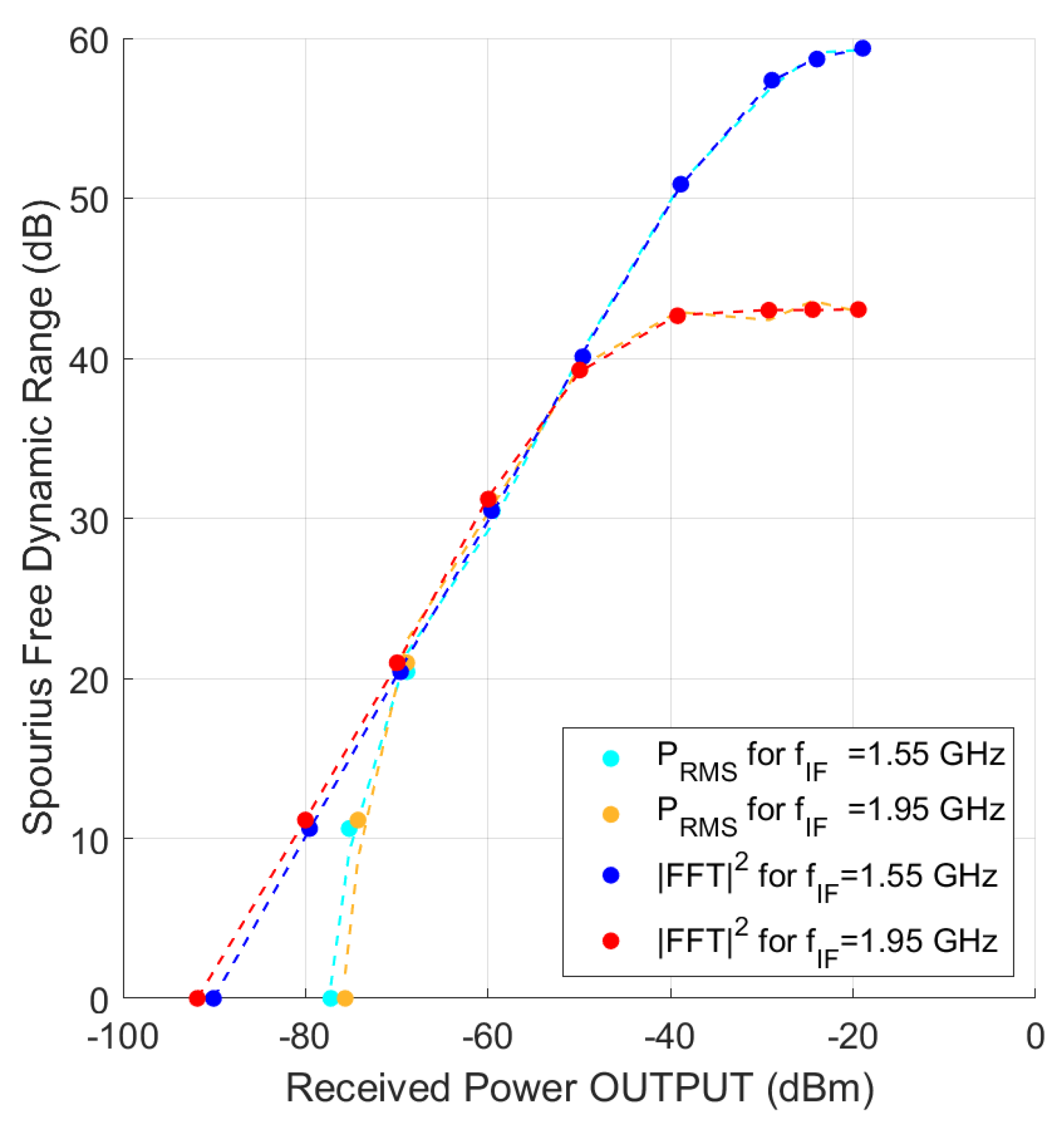
Figure 2.
System calibration set-up: the previously calibrated TX is connected to the RX through a series of WR42 waveguide attenuators, labeled as Att1, Att2, Att3 and Att4 in the picture. Att1 and Att2 introduce a fixed attenuation of 30 and 43 dB, respectively, while Att3 and Att4 provide variable attenuations, ranging from 0 to 30 dB and from 0 to 50 dB, respectively. All the attenuators have been previously characterized using a Vector Network Analyzer (VNA).
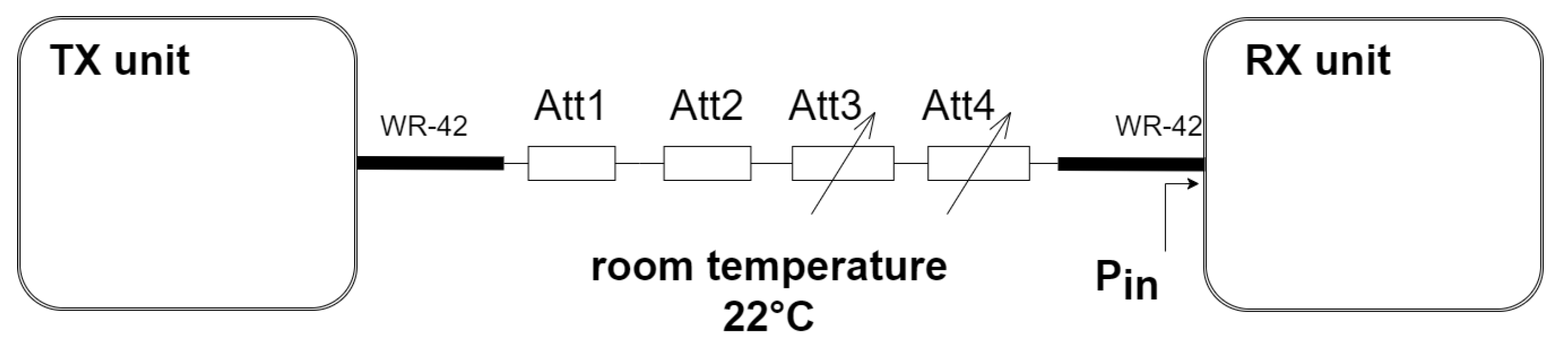
Figure 3.
(a) Uncalibrated receiver output (dBm) versus calibrated power input at the RX antenna terminals at 18.8 GHz (blue) and 19.2 GHz (red) along with their linear regressions (dashed lines). The linear regression equations relating the calibrated (X) and uncalibrated (Y) powers are also plotted for the two channels, as well as the Pearson correlation coefficient R; (b) differential attenuation of the TX-RX chain versus total attenuation expected during the measurement campaign. Note that the differential gain of the two antennas has been accounted for.
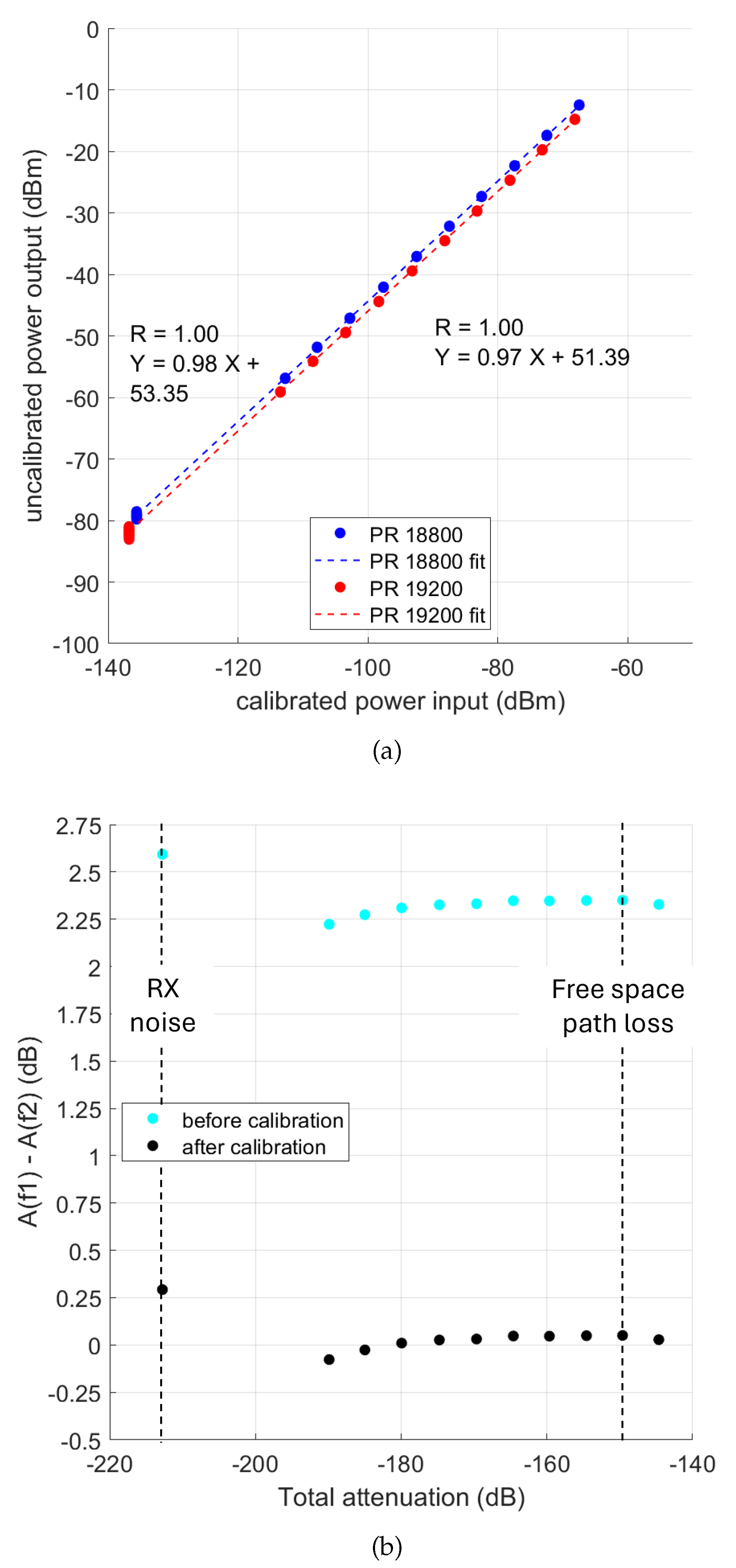
Figure 4.
(a) Residual error versus the internal TX temperature; (b) differential gain of the entire RX chain versus the external temperature, before (red) and after correction (blue). The linear regression equations relating temperature (X) and differential gain (Y) are also plotted for the two channels, as well as the Pearson correlation coefficient R.
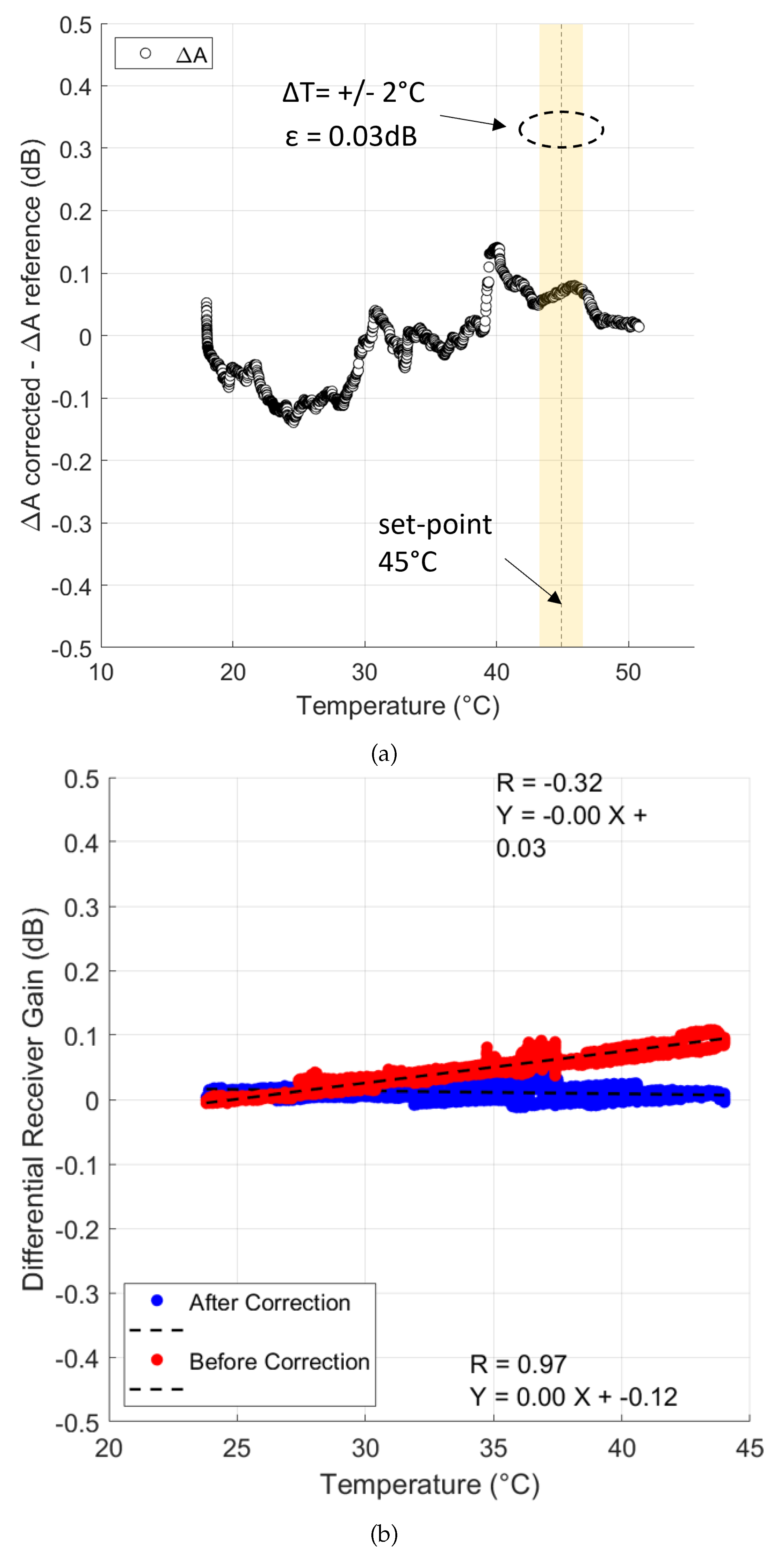
Figure 6.
Geographical arrangement of the measurement instruments. The red line represents the radio link between the TX (44.1277° lat., 10.6434° lon., 1880 meters a.s.l.) and the RX (43.7985° lat., 11.2528° lon., 60 meters a.s.l.). The blue stars indicate the positions of the four ground weather stations considered for the joint data analysis (see Table 2).
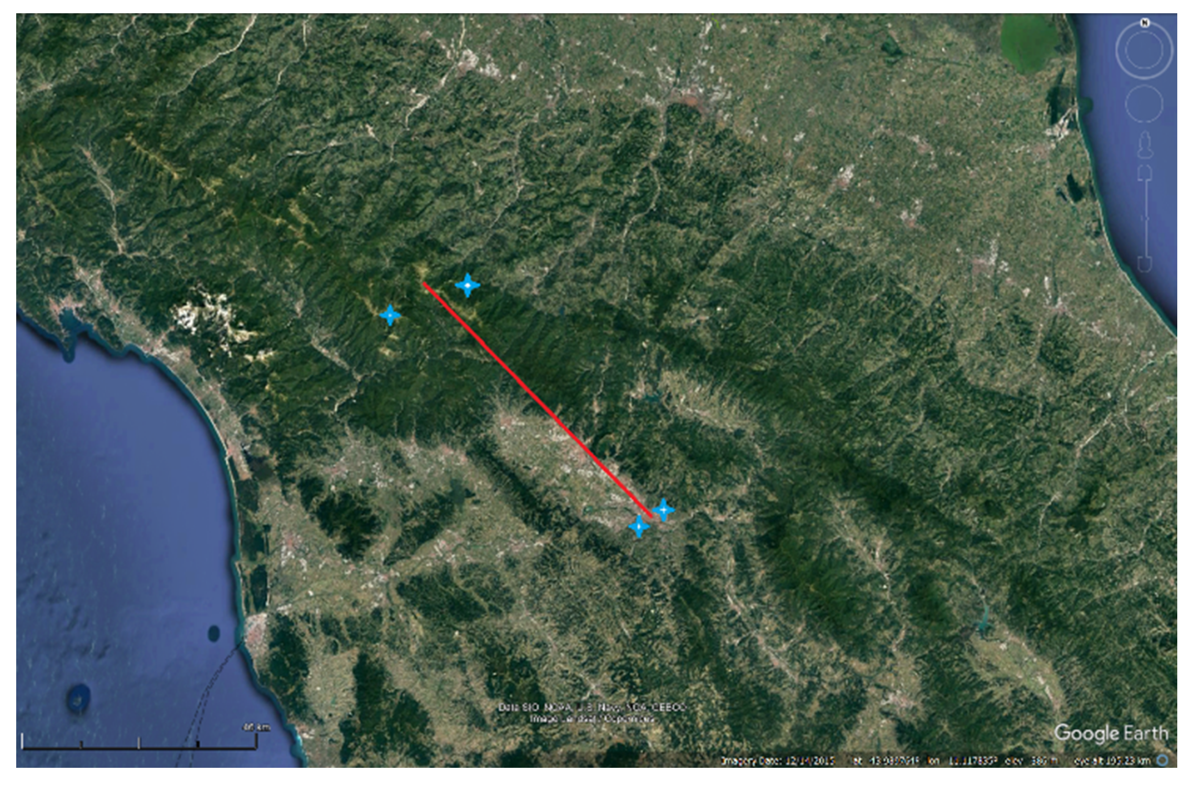
Figure 7.
Webcam view from the TX site towards the RX site taken on Aug 1st, 2022, 07.00 UTC.
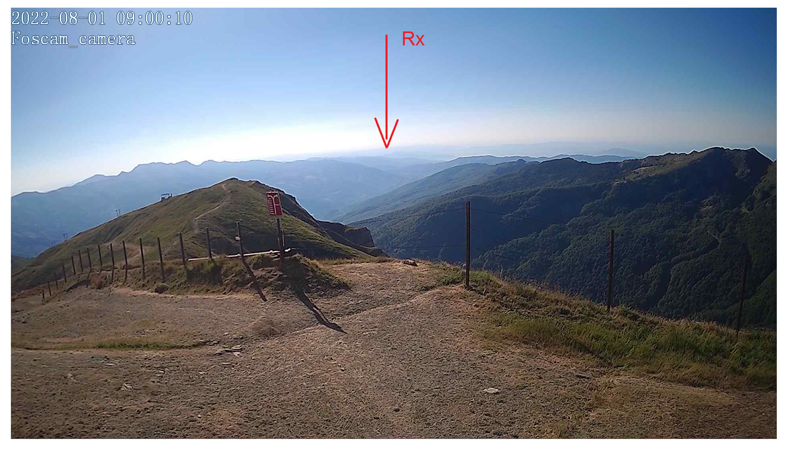
Figure 8.
Campaign data in a single snapshot. RX temp: mean value of the temperatures measured by the stations RX1 and RX2. TX temp: mean value of the temperatures measured by the stations TX1 and TX2. RAIN: 0 no rainfall; -10 rainfall in at least one of the four weather stations. 18.8 GHz Ch and 19.2 GHz Ch: received powers at the two NDSA channels. and : the IWV computed by the SWAMM-2 instrument with 10 s and 1 hour integration interval, respectively. : the IWV computed through Equation (4).
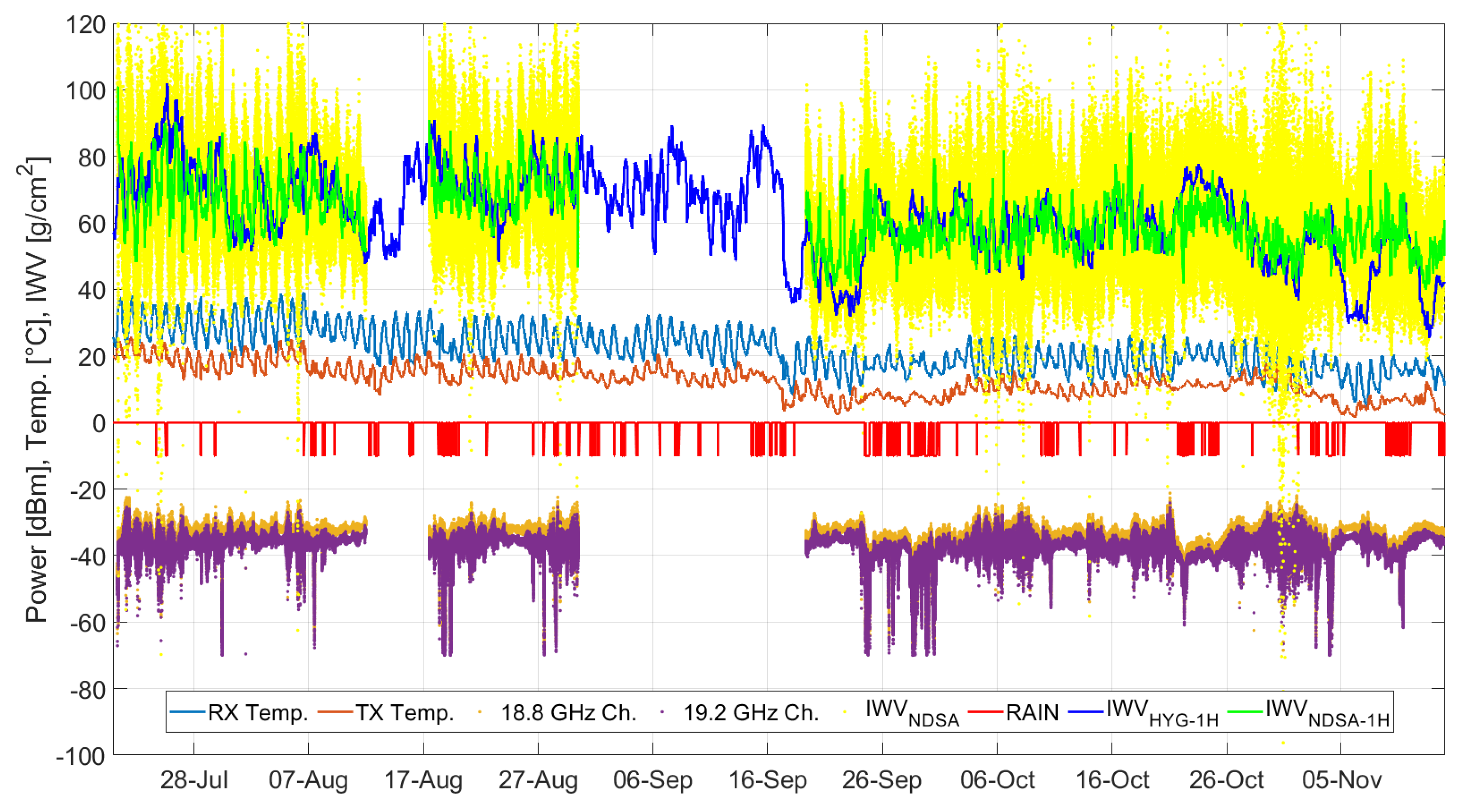
Figure 9.
Aug, 7, 2022. Effects of heavy rainfall.
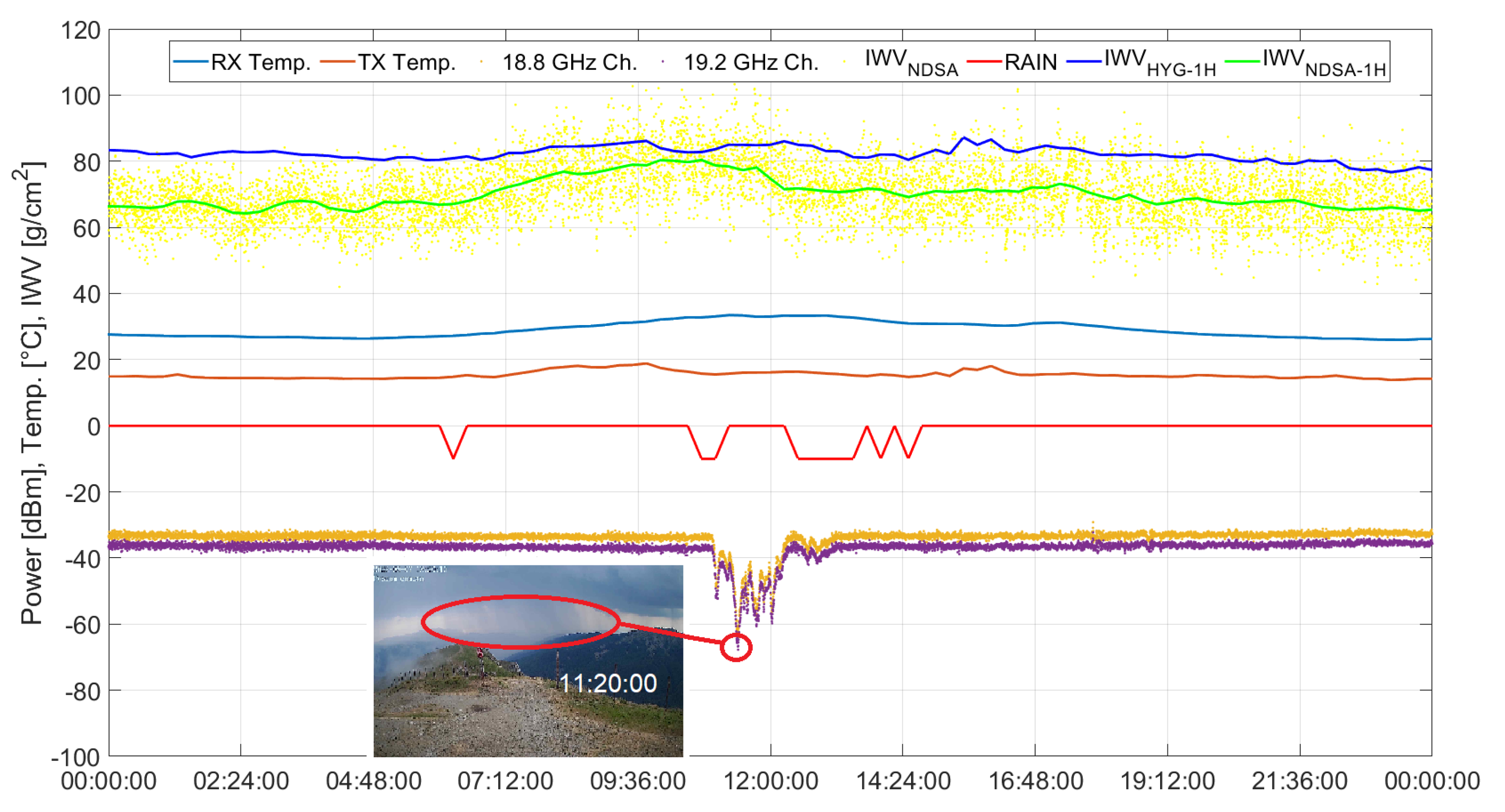
Figure 10.
July, 28, 2022. Effects of light rainfall.
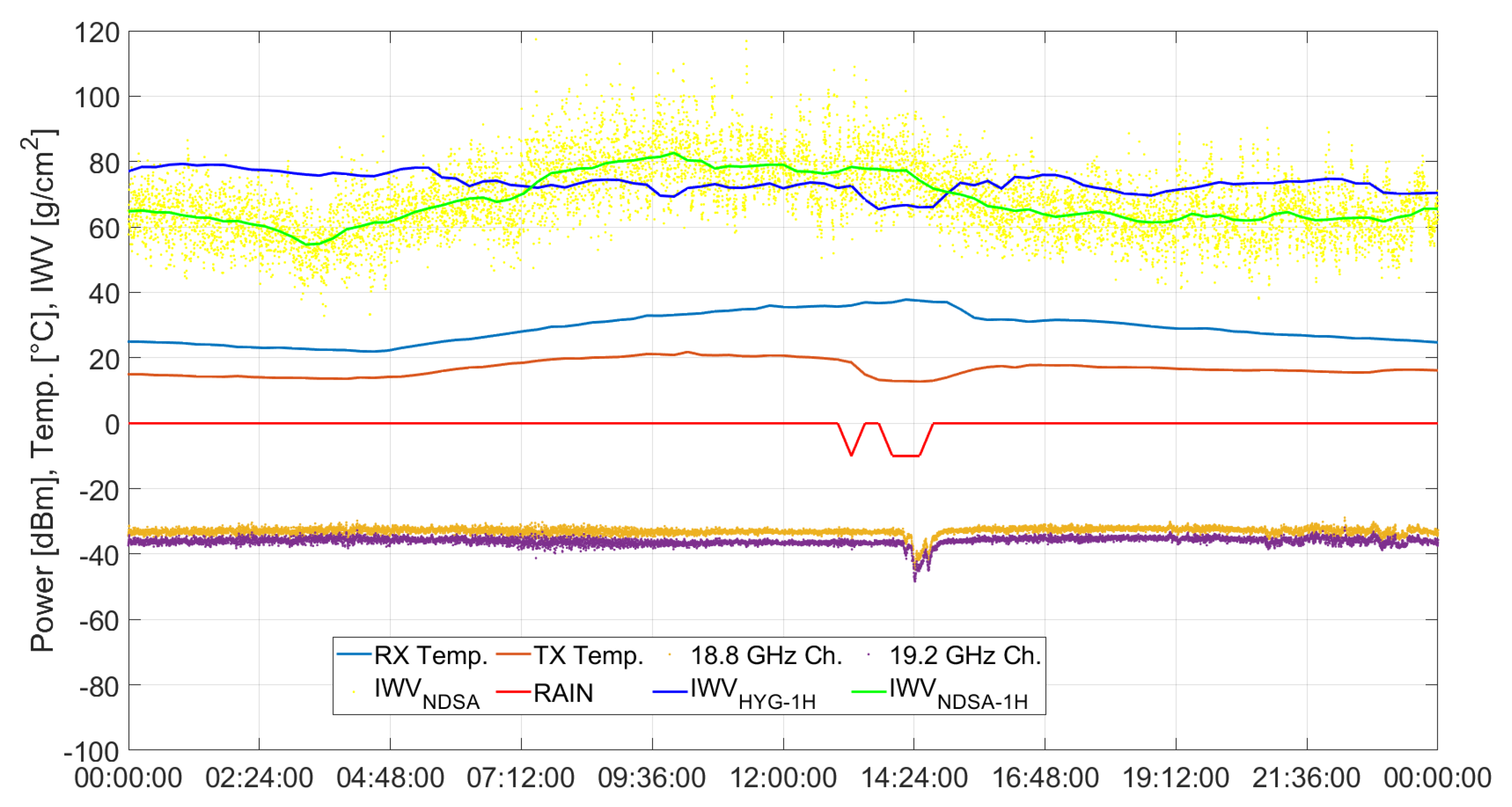
Figure 11.
October, 21 2022. Effects of clouds and fog.
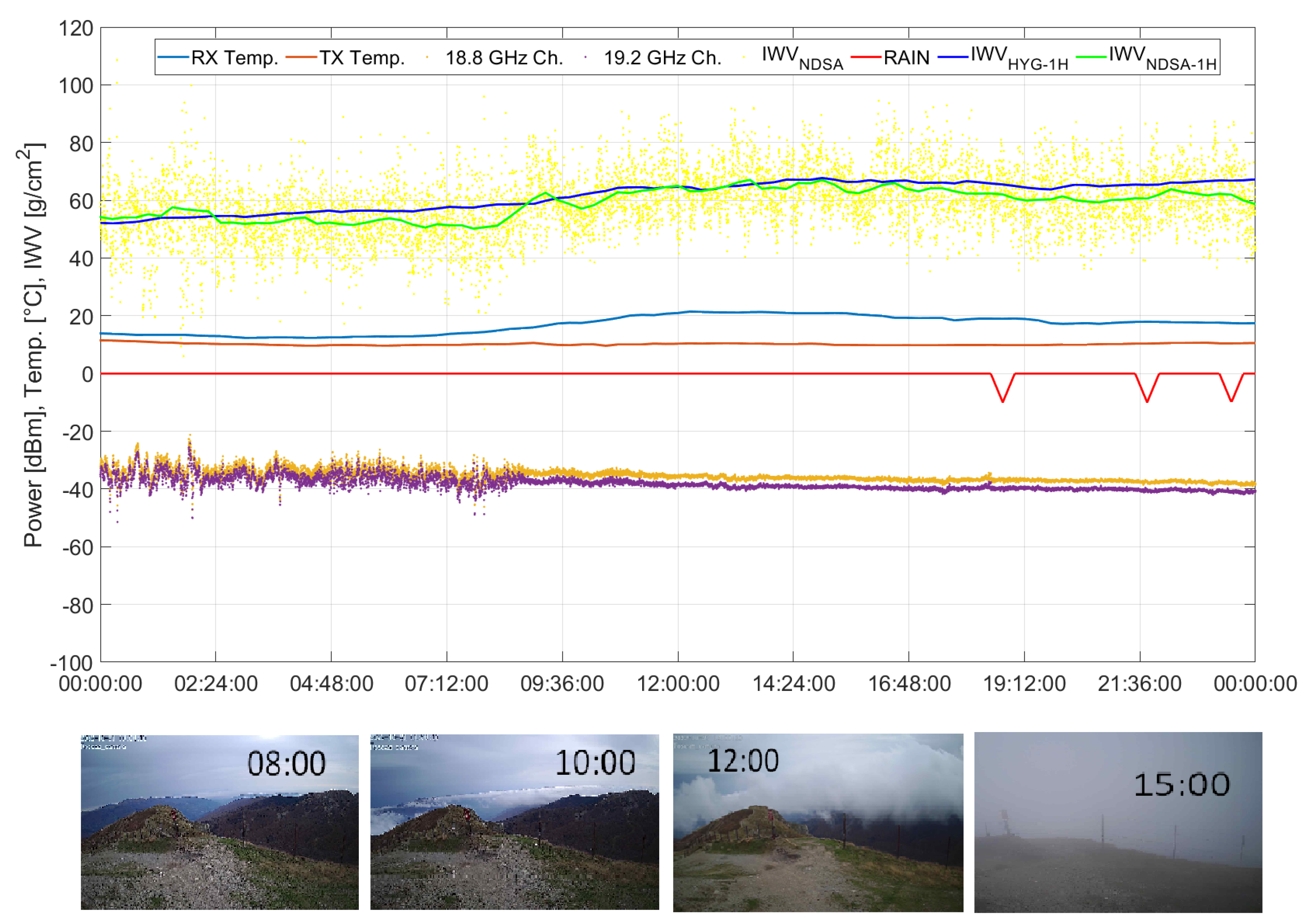
Figure 12.
Campaign data from July 31 to August 6, 2022.
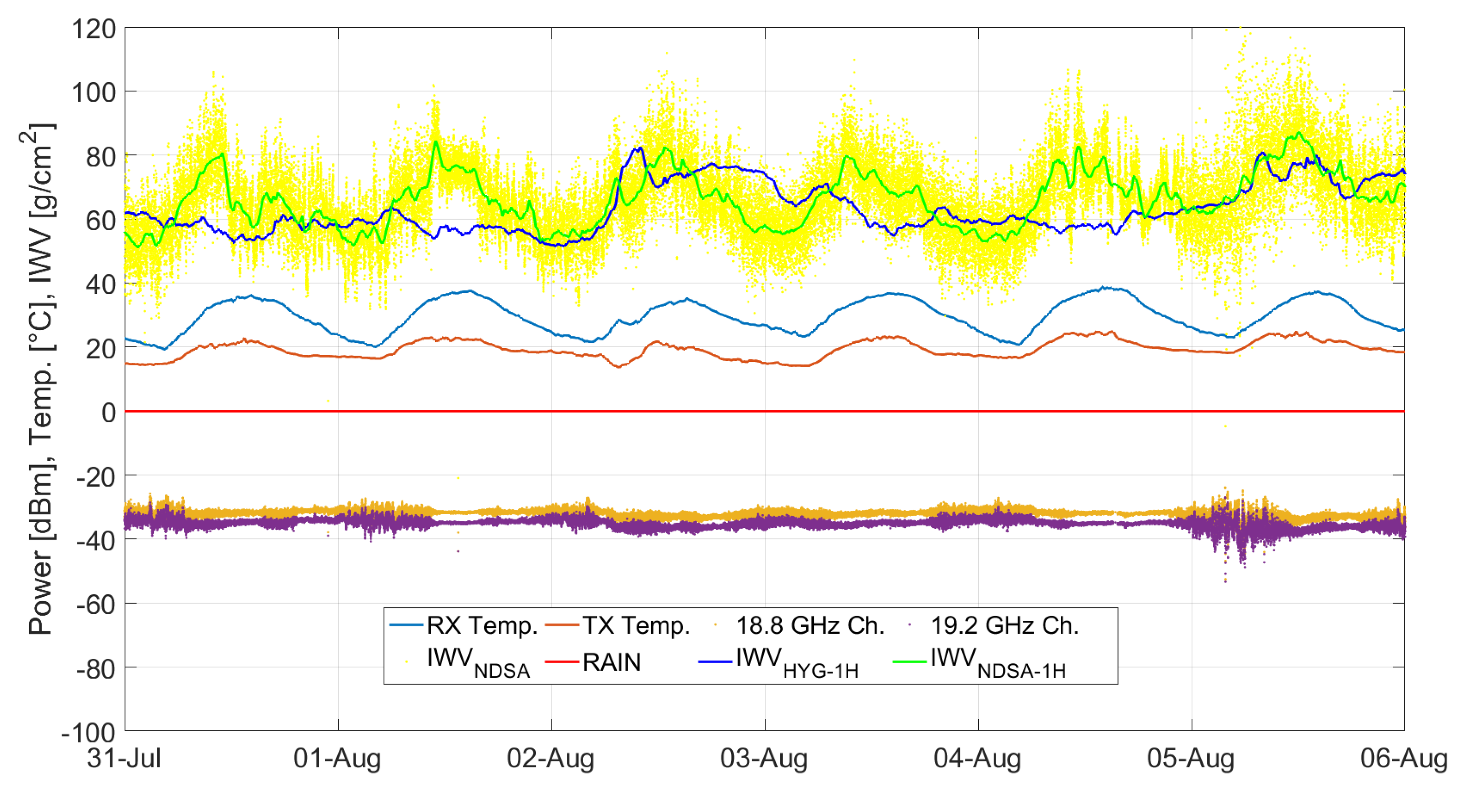
Figure 13.
Temperature (red markers) and relative humidity (blue markers) recorded by the weather station TX1 versus that recorded by station TX2.
Figure 13.
Temperature (red markers) and relative humidity (blue markers) recorded by the weather station TX1 versus that recorded by station TX2.
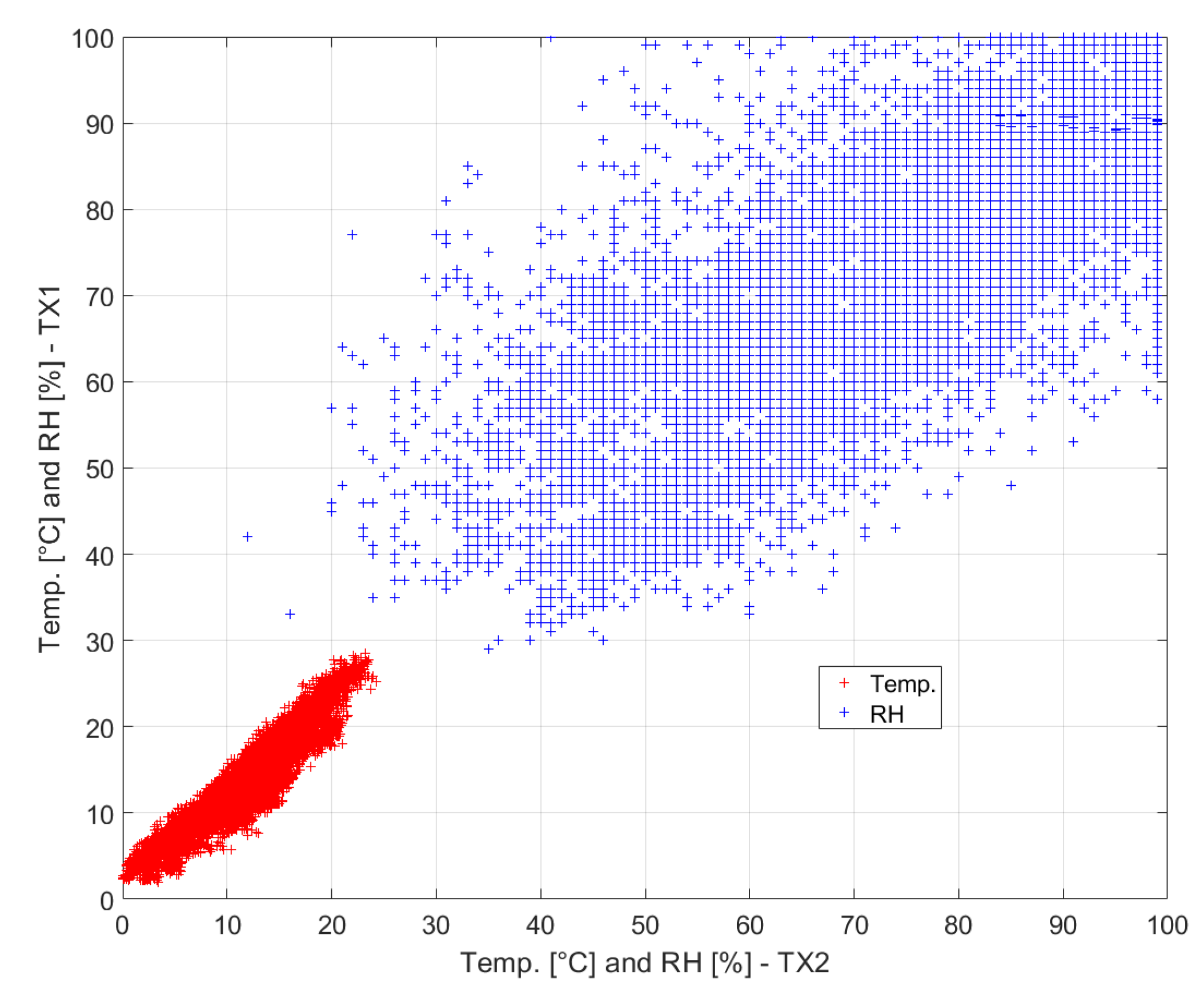
Figure 14.
Temperature (red markers) and relative humidity (blue markers) recorded by the weather station RX1 versus that recorded by station RX2.
Figure 14.
Temperature (red markers) and relative humidity (blue markers) recorded by the weather station RX1 versus that recorded by station RX2.
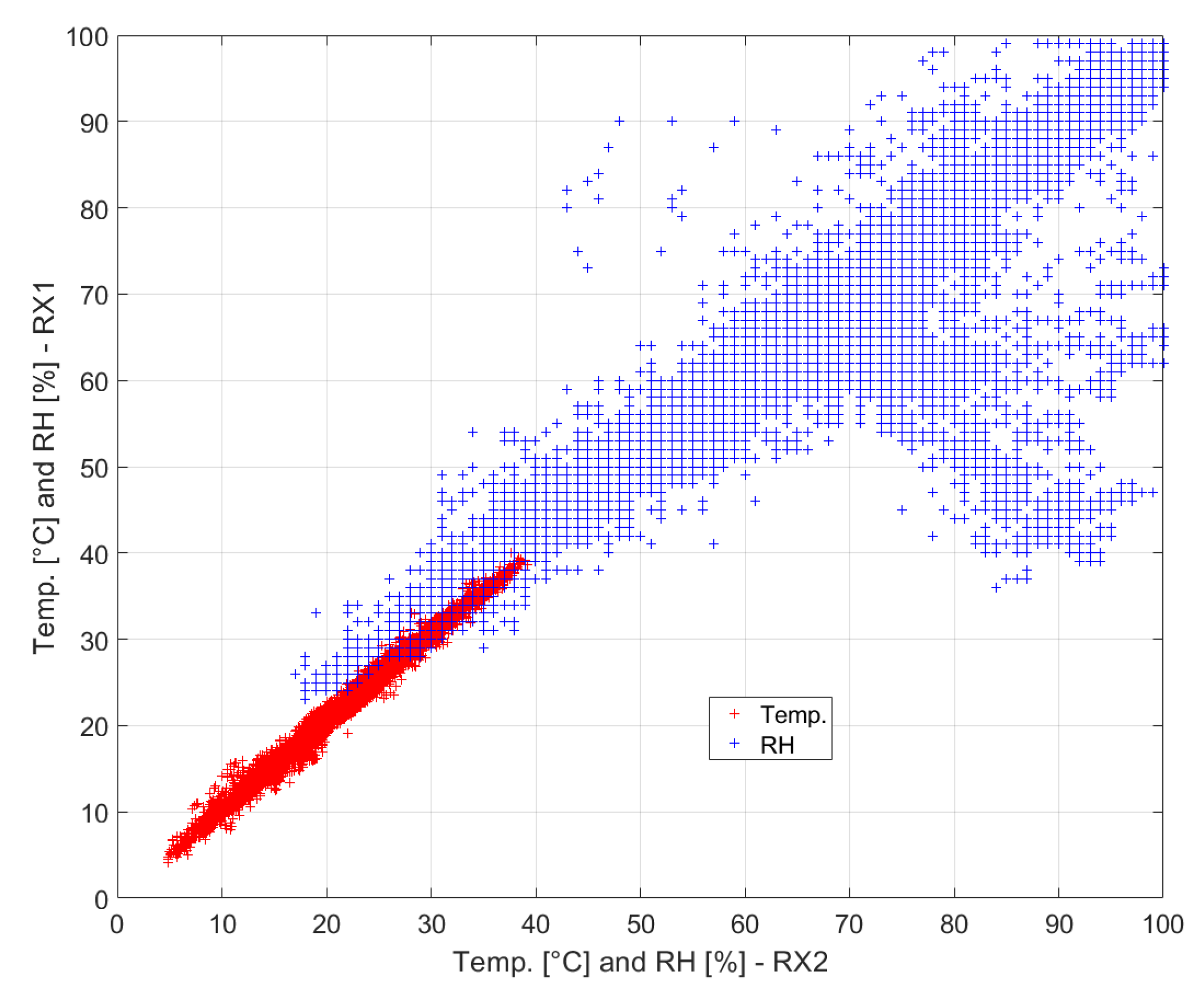
Figure 15.
Campaign data from Aug. 23 to Aug. 30, 2022.
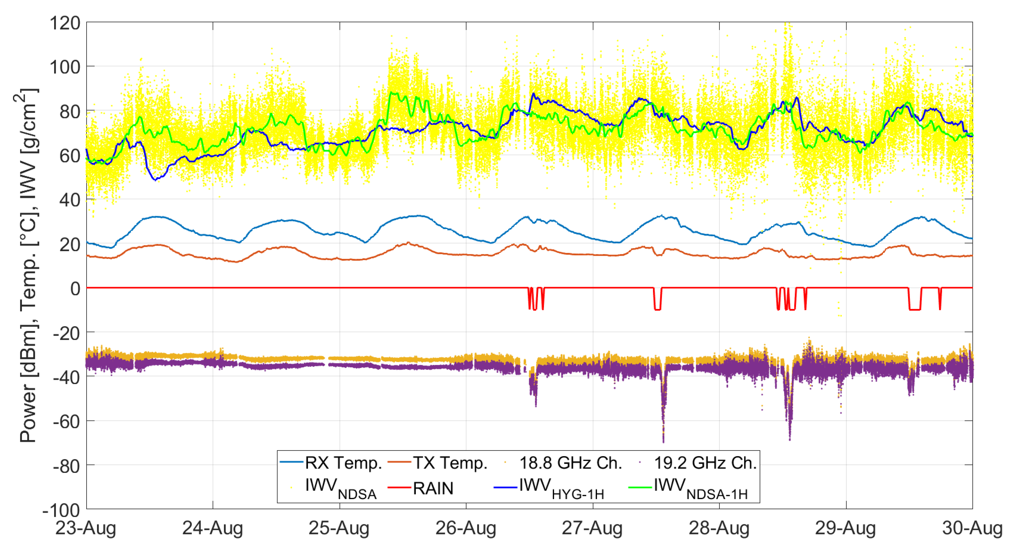
Figure 16.
Campaign data from Oct. 1 to Oct. 8, 2022.
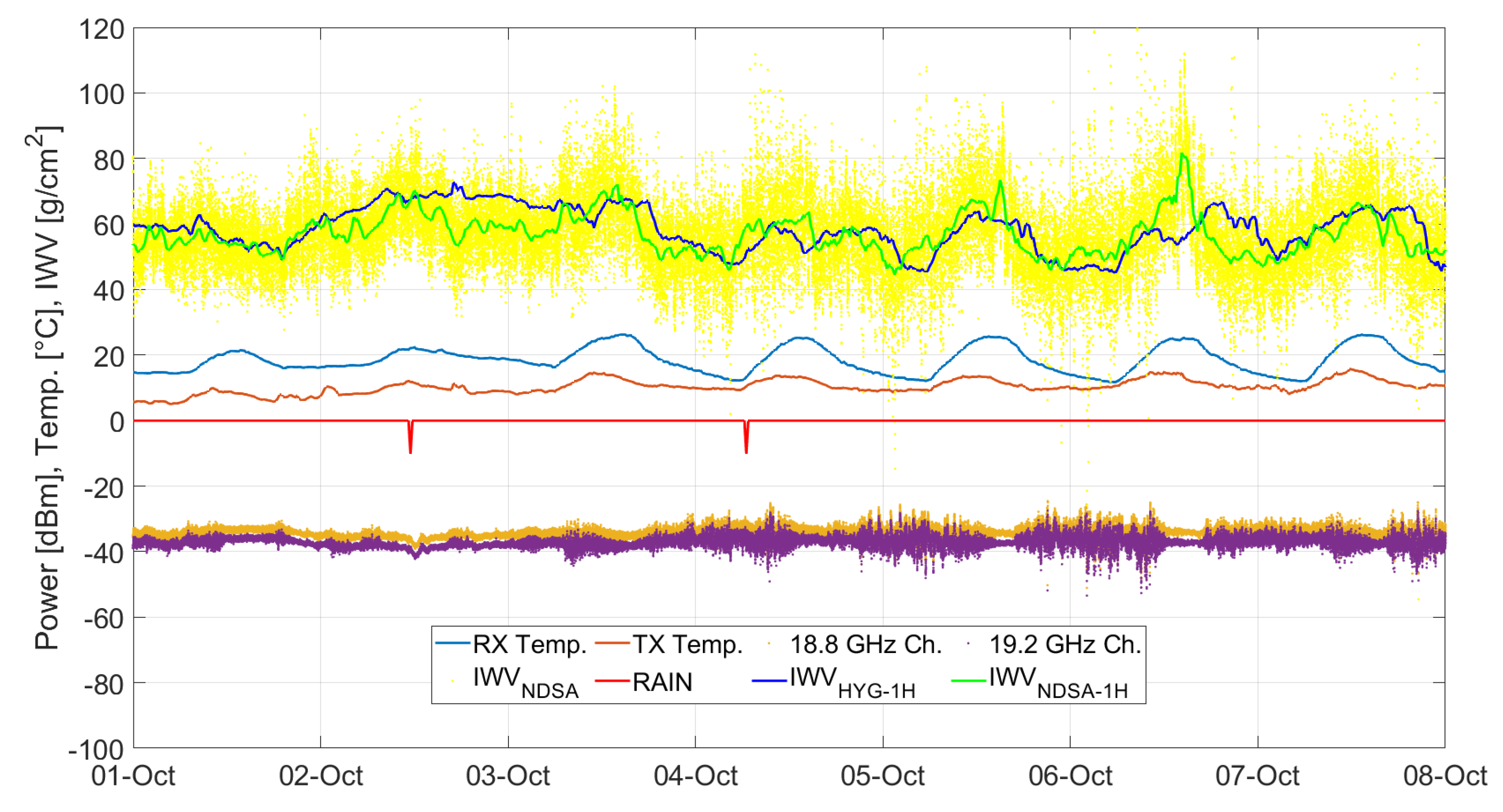
Figure 17.
Spectral sensitivity measured by the SWAMM-2 instrument vs. derived from the ground station data.
Figure 17.
Spectral sensitivity measured by the SWAMM-2 instrument vs. derived from the ground station data.
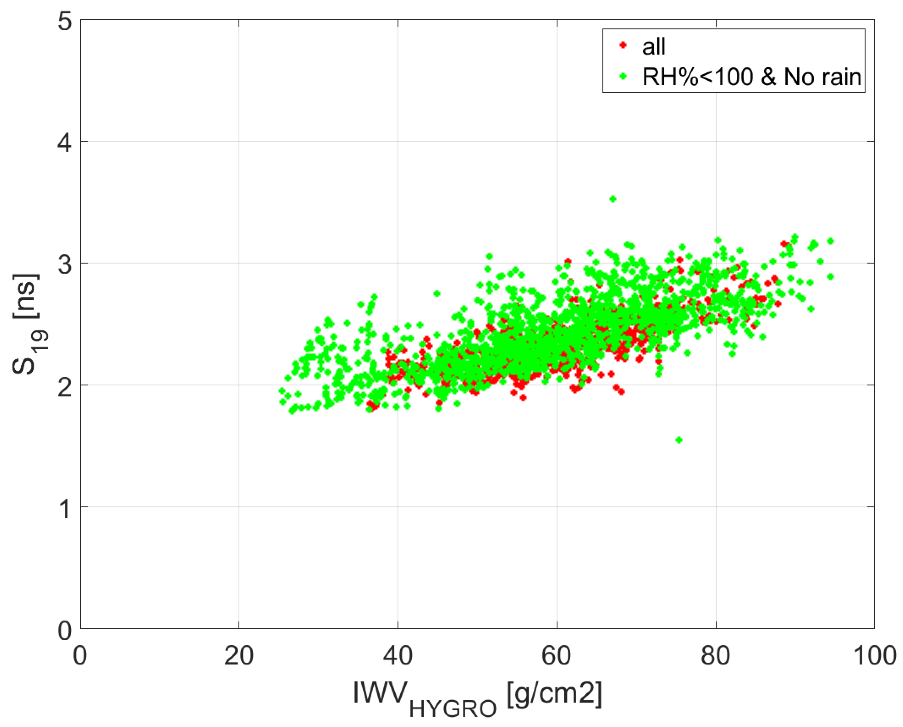

Table 1.
Instrumental uncertainties of the TX-RX chain expected during the measurement campaign.
| Type | |
|---|---|
| vs. T | 0.03 |
| vs. T | 0.04 |
| RX gain linearity (full range) | 0.12 |
| RX gain linearity (HI SNR) | 0.05 |
| Total (full range) | 0.19 |
| Total (Hi SNR) | 0.12 |
Table 2.
Coordinates of the four weather stations. TX1 and TX2 indicate the weather stations closest to the TX site; RX1 and RX2 indicate the weather stations closest to the RX site.
Table 2.
Coordinates of the four weather stations. TX1 and TX2 indicate the weather stations closest to the TX site; RX1 and RX2 indicate the weather stations closest to the RX site.
| Station ID | Latitude [°] | Longitude [°] | Altitude a.s.l. [m] |
|---|---|---|---|
| RX1 | 43.8193028 | 11.1680350 | 33 |
| RX2 | 43.7987883 | 11.2511400 | 84 |
| TX1 | 44.1390944 | 10.6735397 | 1345 |
| TX2 | 44.1182556 | 10.6092639 | 1674 |
Disclaimer/Publisher’s Note: The statements, opinions and data contained in all publications are solely those of the individual author(s) and contributor(s) and not of MDPI and/or the editor(s). MDPI and/or the editor(s) disclaim responsibility for any injury to people or property resulting from any ideas, methods, instructions or products referred to in the content. |
© 2024 by the authors. Licensee MDPI, Basel, Switzerland. This article is an open access article distributed under the terms and conditions of the Creative Commons Attribution (CC BY) license (http://creativecommons.org/licenses/by/4.0/).
Copyright: This open access article is published under a Creative Commons CC BY 4.0 license, which permit the free download, distribution, and reuse, provided that the author and preprint are cited in any reuse.


