Submitted:
20 August 2024
Posted:
22 August 2024
You are already at the latest version
Abstract
The elasticity of red blood cells (RBCs) is crucial for their ability to fulfill their role in the blood. Decreased RBC deformability is associated with various pathological conditions. This study explores the application of machine learning to predict the elasticity of RBCs using both image data and detailed physical measurements derived from simulations. We simulated RBC behavior in a microfluidic channel. The simulation results provided the basis for generating data on which we applied machine learning techniques. We analyzed the surface-area-to-volume ratio of RBCs as an indicator of elasticity, employing statistical methods to differentiate between healthy and diseased RBCs. The Kolmogorov–Smirnov test confirmed significant differences between healthy and diseased RBCs, though distinctions among different types of diseased RBCs were less clear. We used decision tree models, including random forests and gradient boosting, to classify RBC elasticity based on predictors derived from simulation data. The comparison of the results with our previous work on deep neural networks shows improved classification accuracy in some scenarios. The study highlights the potential of machine learning to automate and enhance the analysis of RBC elasticity, with implications for clinical diagnostics.
Keywords:
red blood cell
; elasticity
; machine learning
; surface-area-to-volume ratio
; decision trees
1. Introduction
The elasticity of red blood cells (RBCs), also referred to as erythrocytes, is one of the key physiological parameters that affect their functionality and ability to perform their primary tasks, such as transporting oxygen and carbon dioxide between the lungs and tissues. They must be able to deform and pass through narrow splenic slits with a width of 1–2 Erythrocytes that are unable to properly squeeze through these splenic slits get trapped and are removed from circulation [1,2]. Loss of RBC deformability accompanies many pathological conditions, such as diabetes, sickle cell anemia, thalassemia, malaria, and others [3,4,5]. Thus, RBC deformability is justified as a physical biomarker of RBC dysfunction. Another area where RBC deformability is important is transfusion medicine, as the loss of RBC deformability is a consequence of RBC aging and storage lesions [6].
The deformability of RBCs is determined by a combination of the viscoelasticity of the plasma membrane, the viscosity of the cytoplasm, and cell geometry [7,8,9,10]. These individual contributions are influenced by a wide range of endogenous and exogenous factors, including the composition and structure of the cell membrane, intracellular factors, physical and chemical environmental conditions, and various pathological states. A recent review study [11] provides a summary of the latest findings on these factors and highlights the need to analyze them in light of the new concept of eryptosis.
In the last decade, machine learning has been increasingly used in the biomedical field to analyze complex biological data and improve diagnostic procedures. In the context of determining the elasticity of RBCs, machine learning brings new possibilities for the analysis of large volumes of data, the identification of subtle patterns and the prediction of the mechanical properties of RBCs.
One of the main uses of machine learning in determining the elasticity of RBCs is the analysis of image data obtained from microscopic measurements. Convolutional neural networks (CNNs) find use in automatic analyzes of microscopic images of RBCs or for segmentation of RBCs from complex images, which is crucial for subsequent analysis [12,13]. CNNs can identify and quantify deformations of RBCs based on their shape and size, thus enabling fast and accurate analysis of large data sets [14].
Machine learning methods are also used to predict the mechanical properties of RBCs based on various input data [15,16]. Various regression or classification models can be trained to predict RBC elasticity based on physiological and biochemical parameters such as ion concentrations, membrane composition and cytoskeleton state. Deep neural networks can process complex data inputs and create predictive models that take into account non-linear relationships between various biological factors and RBC elasticity.
One of the great advantages of using machine learning is the automation of analyses. Machine learning algorithms can be integrated into diagnostic instruments, enabling rapid and accurate analysis of RBC elasticity in a clinical setting. They can also effectively process and analyze big data, which is especially important for population studies and clinical research.
Although machine learning methods offer significant benefits, there are also some limitations and challenges. The most significant limitations include data quality, model interpretability, and overfitting. The accuracy of the models depends on the quality and quantity of input data. Poor quality or incomplete data can lead to erroneous predictions. Some models, especially deep neural networks, can be difficult to interpret, complicating the understanding of biological mechanisms. And in the absence of large enough data sets, models can be overtrained, which leads to weaker generalization to new, independent data.
2. Materials and Methods
2.1. Underlying Computational Model
The source data used to classify the elasticity of red blood cells were obtained from simulation experiments performed using the well-documented PyOIF module [17], which is part of the open-source software package ESPResSo [18]. PyOIF uses a two-component model consisting of fluid and immersed elastic objects to model cell flow. The fluid dynamics is governed by the lattice Boltzmann method (LBM) [19] and the cells are represented using a spring mesh. Both components are linked via a dissipative version of the immersed boundary method (IBM) [20]. In addition to the fluid force, elastic forces act on the points of the cell mesh, which are evaluated from the deformation of the cell, and repulsive forces originating from cell-cell and cell-channel interactions (obstacle or channel wall). At each time step, these forces are summed at each node of the cell membrane and used to propagate the node in space using Newton’s 2nd law of motion. The cells are created of the spring network that is formed by mesh points linked together by five elastic forces. This mesh points models the membrane of the cell, while the inside of the cell is filled with the same fluid as its surroundings. Elastic interactions, which are parameterized by elastic coefficients, model either local elastic properties of the cell membrane (the stretching, bending and local area interactions) or elastic properties related to the whole cell (the global volume and global area interactions).
2.2. Channel Geometry And Flow Setting
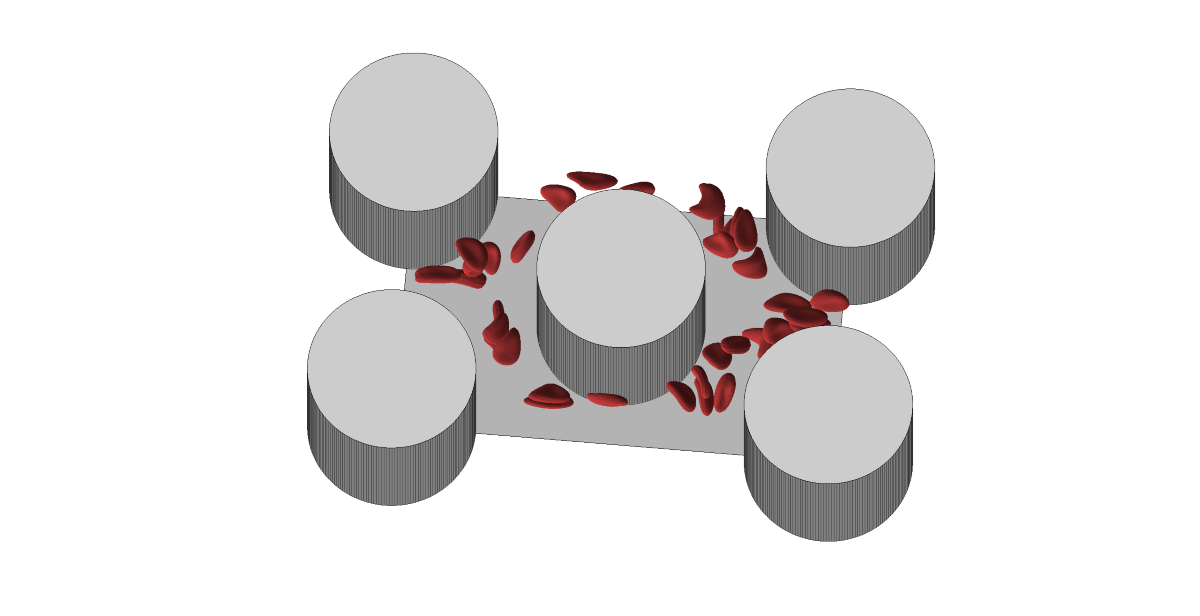
When RBCs come into contact with embedded obstacles, the deformability of RBCs is manifested to a greater extent. Therefore, the proposed microfluidic channel topology contains a periodic array of cylindrical obstacles as in Figure 1. Blood cells have enough space to show their level of deformability during frequent interactions with obstacles. From the entire periodic array of obstacles, only a part consisting of five obstacles was simulated, while the periodic properties of the fluid were ensured in the direction of the fluid flow and in the direction of the channel width. The dimensions of the simulation box were nd the radius of the obstacles was 20m (see Figure 1).
All simulations were performed with consistent channel and fluid flow parameters. They differed only in the initial seeding of cells, with cells placed in random positions in the simulation box. The fluid was discretized into a three-dimensional grid with an edge length of 1 m. We are interested in studying flows in physically relevant cases, therefore the density and viscosity values of the flowing fluid were 1025kg/m3 and 1.3.s, similar to the values of blood plasma. External forces were used to initiate fluid flow with values chosen to achieve a maximum velocity of approximately 0.03m/s.
2.3. Cell Settings
RBCs were represented by a surface mesh consisting of 374 nodes. In the relaxed state, they had dimensions of and their volume and surface were 92.7m3 and 132.9m2, respectively. In this study, four levels of RBC deformability were used, and each level is indicated by the respective values of the stretching coefficient, which has the greatest influence on deformability. All other coefficients had the same values at all levels of deformability. The values of the elastic coefficients of a healthy well-deformable RBC (denoted as ) were determined by calibration based on a biological experiment with optical tweezers [21]. More details about RBC validation can be found in [22]. The values of all the elastic coefficients of the healthy RBC are shown in Table 1. The least deformable RBCs showed rigidity approximately at the level of cells infected with malaria in the schizont stage (denoted as ). The elastic coefficients were chosen by calibration based on the results of experiments in [23]. The remaining two levels of RBC elasticity were equally distributed between healthy and infected RBCs with values of 0.0133 and 0.0216, respectively.
Each simulation involved 36 RBCs, representing nine cells from each level of deformability. Mutual interactions between cells were modeled using the membrane_collision potential with the parameters , , . The interactions between the cells and the walls and obstacles were modeled using the soft_sphere potential with the parameters , , .
3. Summary of Neural Network Results
In the previous study detailed in [24], we investigated the classification of RBCs from video recordings using convolutional neural networks, specifically employing neural networks with ResNet or EfficientNet architectures as the primary backbone. The video recordings were obtained from the simulation described above. The best accuracy was achieved with EfficientNet_v2_B0 as the core model.
We categorized RBCs into four types based on their varying elasticity. Initially, for the task of four-class classification, we achieved an accuracy of 55.48%. However, upon subsequently reducing the target space to two classes, healthy and sick, we attained a significantly improved classification accuracy of 93.91%. Notably, this accuracy outperformed that of training neural networks directly for classifying RBCs into two classes with the final accuracy 61,72%. The results are summarized in Table 2.
These findings led us to hypothesize that RBCs can be effectively segregated into healthy and diseased categories, with the distinction between individual types of diseased RBCs proving to be challenging. Our results suggest a division between healthy and diseased RBCs and the difficulty in distinguishing between specific types of diseased RBCs using current classification methodologies.
4. Statistical Analysis of Elasticity from the Perspective of Red Blood Cell Surface Optimization
One of the typical and key properties of RBCs is to achieve a shape that maximizes its surface for a given volume. We normally describe this value as the surface-area-to-volume () ratio. Although elasticity is a dominant factor for other important properties of RBCs (the ability to penetrate the membrane in healthy RBCs, the clumping of RBCs in sickle-cell anemia, malaria), we were curious about the relationship, whether and how the different elasticity of RBCs would statistically manifest and differ in values of the parameter . Articles [7,8] show that similar research and results can be obtained when studying the behavior of real RBCs. We investigated the relationship between RBC volume and surface area in our simulation model in [25].
4.1. Data and Analysis Tools
The basic data for comparison were calculated and recorded surface and volume values of individual RBCs in the simulation experiment. We are aware that the possibilities of obtaining this data from real experiments are limited and the following analysis is methodologically suitable especially for in silico experiments. Study [7], however, indicates the possibility of measuring values also within in vitro experiments, including their connection to computational experiments. Study [8] also deals with the measurement of and V values.
We deliberately chose the statistical methods of further data processing as simple as possible in order to find out whether even such an approach will already bring relevant results. This simplicity should be somewhat of a counterpoint when compared to the latest machine learning methods.
4.2. Method of Analysis
As an output of the described simulation experiment, for each of the 36 cells with 4 different elasticity values, we used a sequence of 2356 values of its surface and volume during the movement of RBCs in the simulation channel. We recorded the values after every 1000 simulation steps, which corresponded to a displacement of the RBC by an average of 1 to 2 micrometers in the x-axis direction of the channel. From each pair of and V values, we then calculated their ratio and continued to work with this data.
The time series of the parameter for each individual RBC generates interesting graphs (Figure 2), but statistically it is still quite large and confusing data.
We therefore decided to fundamentally reduce the data and for each RBC from all 2356 values of the ratio we selected only their four basic characteristics: maximum, minimum, average and variance of values. Figure 3 shows three of these four characteristics for all nine healthy RBCs.
For each statistic, we thus obtained 4 sets of 9 values for individual groups of RBCs of the same elasticity. Our next goal was to analyze whether it is possible to distinguish between these 4 sets based on these values.
4.3. Analysis Results and Discussion
The combined display of the values of individual statistics for RBCs on Figure 4 indicates that we obtain a good differentiation of healthy RBCs (type 0) from other types for the values of average and maximum of . We do not see a difference for minimum and variance of values, and we do not see a clear distinction between the three types of RBCs with reduced elasticity (type 1 to 3) in any of the statistics.
We verified these observations with the classical Kolmogorov–Smirnov (KS) test for the hypothesis that two given data sets come from the same (unspecified) probability distribution. The results are summarized in Table 3, Table 4, Table 5, Table 6. We reject the mentioned hypothesis for the values of averages and values of maxima when comparing type 0 cells with cells of type 1, 2 or 3. We can reject it at the standard level of significance of 5%, however, except for one case, the p-value is even less than 1%.
Thus, we can conclude that using the elementary statistics of maximum, minimum, average and variance and the basic KS test, we can significantly differentiate the average and maximum values of the ratio between healthy (type 0) and the other RBCs with reduced elasticity. We are not able to distinguish between types 1, 2, 3 using these statistics.
We are aware of the limitation of the validity of our conclusion due to the small range of analyzed data given by the design of the simulation experiment. However, we consider the simplicity of the proposed methodology as a benefit, which we can use and verify the conclusions in a larger experiment in-silico and possibly also in-vitro.
On the other hand, we draw the attention to the significant consistency of the obtained conclusions with the results mentioned in Section 3. Those results were obtained using significantly different tools and separate data, although from the same simulation.
The confirmation of the result for the simulation experiments can also be expected based on the verified consistency and robustness of the computational model, when added RBCs or a longer length of their simulated flow should not cause their significantly different behavior.
From the nature of the simulation model and the behavior of the real RBC, it is known that during the described experiment or simulation run, i.e., during the flow of RBC through the channel, the RBC should maintain its volume and its surface may vary. We verified this assumption statistically (Figure 5) when the variance of surface values of simulated RBCs in the range was approximately one hundred times greater than the variance of volume values in the range . Therefore, the obtained results would be essentially the same if we limited ourselves to examining only the values. This fact can be used to partially simplify the design of the necessary experiments or requirements for their output data.
5. Classification Using Decision Trees
In [24], we dealt with the question of whether it is possible to classify RBC stiffness using deep learning based on analyzing the video recording of the flow of RBCs, and what accuracy the classification can be achieve in this way. Video recording is relatively easy to obtain. However, if we had available more detailed data on cell movement, which can be obtained, e.g., by recording the flow from several sides or using different sensors, it can be expected that the classification accuracy would be improved.
If we use video images directly for classification, it is natural to choose deep neural networks as the model. However, in the case where we have specific properties of the captured cell available as data, describing its shape, speed, and changes in these properties over time, it makes sense to apply models that are suitable for working with tabular data. The simulation from which we generated the videos can be as well used to generate such data. Before investing into experiments with expensive sensors, we can thus verify the classification accuracy that can theoretically be expected with such a procedure. At the same time, we will be able to compare the classification ability of individual models and also evaluate which predictors have a significant impact on classification accuracy. This can be important when designing real experiments.
5.1. Used Predictors
We use cell triangulation to calculate predictors from the simulation. The output of the simulation for each cell is the position of each of the 374 triangulation nodes, determined by three coordinates in three-dimensional space. Various characteristics can be calculated from this data, which we subsequently use as predictors in classification. In total, we created 41 predictors. We divided them into several sets according to the estimated complexity of obtaining them from a real experiment. Based on this, we created 6 tests ordered according to the number of predictors we use. In the first test, we use only the most easily obtainable predictors, while in the final test, we use all of them:
- The 1st set consists of only two predictors: the dimensions of the rectangle in which the monitored cell is located, i.e., dimension of the cell in the direction of the x-axis and in the direction of the y-axis. These values can be easily obtained from a (static) snapshot of the cell.
- In the 2nd set, the additional predictors are velocities and changes in the velocity of the cell in the x- and y-directions. These data can be calculated from several consecutive images.
- The 3rd set also includes dimensions and velocities in the z-axis direction. These values can be obtained from images taken from a different angle.
- To the 4th set, we added the cell axis length and the maximum and minimum diameter of the cell equator, which can potentially be determined from multi-angle images.
- The 5th set additionally contains predictors that can be calculated from the complete cell triangulation: cell surface, cell volume and means, standard deviations and skewness coefficients calculated from the lengths of all triangulation edges, angles formed by every two triangulation triangles and solid angles at all triangulation nodes. Cell triangulation is quite difficult to obtain from a real experiment, it would require the creation of a 3D image of the cell from the scanned flow.
- The 6th set also contains means, standard deviations and coefficients of skewness of deviations and absolute deviations of the characteristics added in the 5th set. The deviations are calculated from the cell in a relaxed state, so for the calculation we need to have the basic triangulation of the cell, which in our procedure corresponds to the cell in the first step of the simulation.
The mentioned predictors correspond to the current state of the cell at one monitored moment (in one step of the simulation). During experiments, however, we have the opportunity to observe the cell longer during several steps. It can be expected that the classification accuracy will improve if we track the cell longer. To assess this effect, for each , and 1280, we created a model in which we monitored each cell for simulation steps, with the simulation record saved once per 1000 steps. (Note that one pass of a cell through the channel corresponds to approximately 100000 simulation steps.) Since the values of the individual predictors change during the movement of the cell through the channel, we have S values for each predictor instead of just one value. From these values, we calculated the mean and standard deviation and used them as predictors – in total, we have two predictors for each value described in the bulleted list above (with the exception of the case of , where we only work with static snapshots of the cells).
5.2. Used Machine Learning Tools
Given the nature of the data (number of predictors, high correlation of some predictors), we consider models based on decision trees, which usually achieve the best results for tabular data [30,31], to be a suitable tool for classification. We used two of the most popular techniques: random forest and gradient decision trees. For the implementation, we used the Python language and the methods RandomForestClassifier from the sklearn library and XGBClassifier from the xgboost library.
The goal in this section was not to maximize the accuracy to the highest possible level, therefore we did not optimize the hyperparameters of individual models and were satisfied with the default values.
For each of the six sets of predictors and each of the nine S values, we trained 2 models using both methods – one for classification into four classes (four types of cell stiffness), the other for classification into two classes (healthy/diseased cell). When evaluating the accuracy of the classification into two classes, in addition to the second model, we also used the first model, in which we combined the three types of stiffness into the result "diseased cell" (similarly, as we did in [24]).
5.3. Data Preparation
We sampled the simulation for each recorded simulation step, after which followed at least additional steps (so that we could calculate predictors for a given value of S). However, we removed the first 100000 steps of the simulation. The total number of generated samples is thus equal to , where C is the total number of cells in the simulation and N is the total number of recorded simulation steps. (We remind you that every 1000th step is recorded, so the total number of steps is approx. .)
It follows from the above that many generated samples are very similar to each other. The reason is, that the cell changes little between two consecutive steps, moreover, for , two samples recorded close to each other have a large part of the data from which we generate the predictors in common (the last recorded steps of the sample are identical to the first recorded steps of the following sample). This must be kept in mind when dividing the set into a possible training and validation or testing part – it is not appropriate to use data from one simulation in several parts and a new simulation must be used each time.
Due to the tree models used and the omission of hyperparameter optimization, we did not need the validation part, so we we only needed two simulations. We created training samples from the simulation with values of and , the total number of training samples is thus in the range from 81216 (for ) to 35172 (for ). The second simulation, from which we generated test samples, has parameters and , so the number of samples is in a similar range (from 78804 for to 32760 for ).
We recall that the simulations are the same as we used in [24], that is, there are 9 cells from each class among the 36 cells.
5.4. Classification Results
Let us first have a look at the classification accuracy based on the value of S, that is, let us analyze the effect of the number of steps we monitor each cell. From the plots in Figure 6, Figure 7, it can be concluded that increasing S has a positive effect up to the level around the values of or 320, from which the classification accuracy ceases to improve continuously. Thus, it seems pointless to track the cell for significantly longer than one pass through the channel (approx. 100000 simulation steps).
The plots in Figure 8, Figure 9 show how the classification accuracy changes depending on which set of predictors we use. Especially when classifying into 4 classes, a significant improvement in accuracy can be observed when moving from the 4th set to the 5th set. On the other side, the effect of the third dimension (the transition from the 2nd set to the 3rd set) does not seem to be very significant.
In all Figure 6, Figure 7, Figure 8 and Figure 9, the dashed line shows the accuracy we achieved in the classification using deep neural networks in [24]. Within that approach, we observed each cell during one passage through the channel, which corresponds approximately to a model with . In Figure 8 in the middle plot it can be seen that when classifying into 4 classes, we outperformed neural networks result with the 2nd predictor set. Similarly, the middle plot in Figure 9 shows that in case of 2 classes, we outperformed neural networks with the 4th predictor set.
In [24], we observed a fairly significant difference in the result between a pair of models created for binary classification (healthy/diseased cell). The model that was trained directly for the classification of 2 classes achieved less accuracy (slightly above 60%) than the model trained for the classification of 4 classes, in which we determined the resulting binary classification only by merging the classes containing diseased cells with three different stiffness levels into one class (accuracy above 90%). This strange phenomenon did not appear when decision trees were used – in Figure 7, Figure 9 it can be seen that the accuracy of models trained for the classification of 4 classes (blue and red color) does not differ significantly from the accuracy of models trained directly for binary classification (yellow and purple color).
A comparison of random forest and gradient decision trees does not come out significantly in favor of either method – the results are very similar to each other.
To see which predictors have the biggest impact on the classification, let us take a closer look at the models for (i.e., those where we observe approximately one passage of a cell through the channel) with the 6th set of predictors and the 4th set of predictors. For these models in Figure 10 and Figure 11 we present the significance of the predictors calculated by the permutation_importance method from the sklearn library. In the case of the 6th set and classification into 4 classes, the "edge length delta abs deviation" predictor appears to be the most significant in both models, that is, the predictor indicating the standard deviation of the absolute changes in the lengths of the edges of the triangulation against the relaxed state of the cell. When classifying into 2 classes, "edge angle delta abs mean" and "edge length delta skewness" are significant for both models, that is, the average absolute change in the angles at the edges of the triangulation compared to the relaxed state and the coefficient of skewness of the changes in the lengths of the edges of the triangulation compared to the relaxed state. For the simpler 4th set of predictors, the most significant predictor for all models is the mean of the cell axis length.
5.5. Discussion
Our experiments with decision trees reveal insights into the efficiency of various predictor sets and the impact of recorded sequence length on the classification accuracy. Our results suggest that increasing the length of the sequence (S) generally improves classification accuracy up to a certain point, after which the improvements starts to be negligible. This indicates that while longer observation periods can be beneficial, excessively long monitoring may not yield proportional gains in accuracy. Specifically, monitoring cells for approximately one complete passage through the channel appears sufficient for optimal performance.
The comparison between deep neural networks and decision tree-based models reveals that the latter can achieve comparable or better accuracy with simpler predictor sets. This is particularly evident in the classification into four classes, where decision trees outperformed neural networks using the 2nd predictor set. This confirms that decision trees are a proper tool to effectively handle tabular data, providing a more interpretable and efficient alternative to neural networks.
Future research can focus on several directions to further improve the classification of RBC elasticity. One potential way is the integration of various data sources, such as combining video recordings with additional sensors capturing mechanical properties or biochemical markers of RBCs. This could provide a richer dataset and better classification accuracy. Performing experimental validation using actual RBC samples will be essential to confirm the theoretical findings and translate them into practical diagnostic tools.
Author Contributions
Conceptualization, K.B., H.B. and P.N.; methodology, H.B., P.N. and M.S.; software, S.M., P.N. and M.S.; validation, S.M. and P.N.; formal analysis, H.B. and P.N.; investigation, H.B., S.M. and P.N.; resources, M.S. and H.B.; data curation, S.M., P.N. and M.S.; writing—original draft preparation, H.B., S.M., P.N. and M.S.; writing—review and editing, H.B., K.B., P.N. S.M. and M.S.; visualization, S.M., P.N. and M.S.; supervision, K.B.; project administration, K.B.; funding acquisition, K.B. All authors have read and agreed to the published version of the manuscript.
Funding
This research was supported by the Ministry of Education, Science, Research and Sport of the Slovak Republic under the contract No. VEGA 1/0369/22.
Institutional Review Board Statement
Not applicable.
Informed Consent Statement
Not applicable.
Data Availability Statement
The original data presented in the study are openly available in GitHub at https://github.com/nofto/RBC-Elasticity-Classification. However, the complete output from the simulation is too large for public sharing capabilities and is available on request from the corresponding author.
Acknowledgments
We would like to acknowledge the use of ChatGPT, a generative AI tool, in the preparation of this manuscript. As non-native English speakers, we utilized ChatGPT to assist in the better formulation of several phrases. It is important to note that AI was not employed in the creation of any substantive content within this manuscript. This use of AI is in accordance with MDPI’s guidelines, ensuring full responsibility for the originality, validity, and integrity of the content presented.
Conflicts of Interest
The authors declare no conflicts of interest.
Abbreviations
The following abbreviations are used in this manuscript:
| CNN | convolutional neural network |
| IBM | immersed boundary method |
| KS test | Kolmogorov–Smirnov test |
| LBM | lattice Boltzmann method |
| RBC | Red blood cell |
References
- Klei, T. R. L.; Dalimot, J.; Nota, B.; Veldthuis, M.; Mul, F. P. J.; Rademakers, T.; Hoogenboezem, M.; Nagelkerke, S. Q.; van Ijcken, W. F. J.; Oole, E; Svendsen, P.; Moestrup, S. K.; van Alphen, F. P. J.; Meijer, A. B.; Kuijpers, T. W.; van Zwieten, R; van Bruggen, R. Hemolysis in the spleen drives erythrocyte turnover. Blood 2020, 136, 1579–1589. [CrossRef]
- Duez, J.; Holleran, J.P.; Ndour, P.A.; Pionneau, C.; Diakité, S.; Roussel, C.; Dussiot, M.; Amireault, P.; Avery, V.M.; Buffet, P.A. Mechanical clearance of red blood cells by the human spleen: Potential therapeutic applications of a biomimetic RBC filtration method. Transfus. Clin. Biol. 2015, 22, 151–157. [Google Scholar] [CrossRef]
- Tyas, D.A.; Hartati, S.; Harjoko, A.; Ratnaningsih, T. Morphological, texture, and color feature analysis for erythrocyte classification in thalassemia cases. IEEE Access 2020, 8, 69849–69860. [Google Scholar] [CrossRef]
- Alapan, Y.; Matsuyama, Y.; Little, J.A.; Gurkan, U.A. Dynamic deformability of sickle red blood cells in microphysiological flow. Technology 2016, 4, 71–79. [Google Scholar] [CrossRef] [PubMed]
- Depond, M.; Henry, B.; Buffet, P.; Ndour, P.A. Methods to investigate the deformability of RBC during malaria. Front. Physiol. 2020, 10, 1613. [Google Scholar] [CrossRef] [PubMed]
- Islamzada, E.; Matthews, K.; Guo, Q.; Santoso, A.T.; Duffy, S.P.; Scott, M.D.; Ma, H. Deformability based sorting of stored red blood cells reveals donor-dependent aging curves. Lab on a Chip 2020, 20, 226–235. [Google Scholar] [CrossRef] [PubMed]
- Namvar, A.; Blanch, A.J.; Dixon, M.W.; Carmo, O.M.S.; Liu, B.; Tiash, S.; Looker, O.; Andrew, D.; Chan, L.; Tham, W.; Lee, P.V.S.; Rajagopal, V.; Tilley, L. Surface area-to-volume Ratio, Not Cellular Viscoelasticity, Is the Major Determinant of Red Blood Cell Traversal Through Small Channels. Cell. Microbiol. 2021, 23, e13270. [Google Scholar] [CrossRef]
- Renoux, C.; Faivre, M.; Bessaa, A.; Da Costa, L.; Joly, P.; Gauthier, A.; Connes, P. Impact of Surface-area-to-volume Ratio, Internal Viscosity and Membrane Viscoelasticity on Red Blood Cell Deformability Measured in Isotonic Condition. Sci. Rep. 2019, 9, 6771. [Google Scholar] [CrossRef]
- Park, H.; Lee, S.; Ji, M.; Kim, K.; Son, Y.; Jang, S.; Park, Y. Measuring cell surface area and deformability of individual human red blood cells over blood storage using quantitative phase imaging. Sci. Rep. 2016, 6, 34257. [Google Scholar] [CrossRef]
- Diez-Silva, M.; Dao, M.; Han, J.; Lim, C.T.; Suresh, S. Shape and biomechanical characteristics of human red blood cells in health and disease. MRS Bull. 2010, 35, 382–388. [Google Scholar] [CrossRef]
- Brun, J.F.; Varlet-Marie, E.; Myzia, J.; de Mauverger, E.R.; Pretorius, E. Metabolic influences modulating erythrocyte deformability and eryptosis. Metabolites 2022, 12, 4. [Google Scholar] [CrossRef]
- Lamoureux, E.S.; Cheng, Y.; Islamzada, E.; Matthews, K.; Duffy, S.P.; Ma, H. Biophysical Profiling of Red Blood Cells from Thin-film Blood Smears using Deep Learning. Heliyon 2024, 0, e35276. [Google Scholar] [CrossRef] [PubMed]
- Molina, A.; Rodellar, J.; Boldú, L.; Acevedo, A.; Alférez, S.; Merino, A. Automatic identification of malaria and other red blood cell inclusions using convolutional neural networks. Comput. Biol. Med. 2021, 136, 104680. [Google Scholar] [CrossRef] [PubMed]
- Lopes, M. G.; Recktenwald, S.M.; Simionato, G.; Eichler, H.; Wagner, C.; Quint, S.; Kaestner, L. Big data in transfusion medicine and artificial intelligence analysis for red blood cell quality control. Transfus. Med. Hemother. 2023, 50, 163–173. [Google Scholar] [CrossRef] [PubMed]
- Aliyu, H.A.; Sudirman, R.; Razak, M.A.A.; Abd Wahab, M.A. Red blood cell classification: deep learning architecture versus support vector machine. In Proceedings of the 2nd international conference on biosignal analysis, processing and systems (ICBAPS), Kuching, Malaysia, 24–26 July 2018; pp. 142–147. [Google Scholar] [CrossRef]
- Singh, V.; Srivastava, V.; Mehta, D.S. Machine learning-based screening of red blood cells using quantitative phase imaging with micro-spectrocolorimetry. Opt. Laser Technol. 2020, 124, 105980. [Google Scholar] [CrossRef]
- Jančigová, I.; Kovalčíková, K.; Weeber, R.; Cimrák, I. PyOIF: Computational tool for modelling of multi-cell flows in complex geometries. PLoS Comput. Biol. 2020, 16, e1008249. [Google Scholar] [CrossRef]
- Weik, F.; Weeber, R.; Szuttor, K.; Breitsprecher, K.; de Graaf, J.; Kuron, M.; Landsgesell, J.; Menke, H.; Sean, D.; Holm, C. ESPResSo 4.0 – an extensible software package for simulating soft matter systems. Eur. Phys. J. Spec. Top. 2019, 227, 1789–1816. [Google Scholar] [CrossRef]
- Krüger, T.; Kusumaatmaja, H.; Kuzmin, A.; Shardt, O.; Silva, G.; Viggen, E.M. The lattice Boltzmann method; Springer International Publishing: Switzerland, 2017. [Google Scholar] [CrossRef]
- Bušík, M.; Slavík, M.; Cimrák, I. Dissipative coupling of fluid and immersed objects for modelling of cells in flow. Comput. Math. Methods Med. 2018, 2018, 7842857. [Google Scholar] [CrossRef]
- Mills, J.P.; Qie, L.; Dao, M.; Lim, C.T.; Suresh, S. Nonlinear elastic and viscoelastic deformation of the human red blood cell with optical tweezers. MCB Mol. Cell. Biomech. 2004, 1, 169. [Google Scholar] [CrossRef]
- Jančigová, I.; Kovalčíková, K.; Bohiniková, A.; Cimrák, I. Spring-network model of red blood cell: From membrane mechanics to validation. Int. J. Numer. Methods Fluids 2020, 92, 1368–1393. [Google Scholar] [CrossRef]
- Suresh, S.; Spatz, J.; Mills, J.P.; Micoulet, A.; Dao, M.; Lim, C.T.; Beil, M.; Seufferlein, T. Connections between single-cell biomechanics and human disease states: gastrointestinal cancer and malaria. Acta Biomater. 2005, 1, 15–30. [Google Scholar] [CrossRef]
- Molčan, S.; Smiešková, M.; Bachratý, H.; Bachratá, K.; Novotný, P. Classification of red blood cells using time-distributed convolutional neural networks from simulated videos. Appl. Sci. 2023, 13, 7967. [Google Scholar] [CrossRef]
- Cimrák, I.; Bachratá, K.; Bachratý, H.; Jančigová, I.; Tóthová, R.; Bušík, M.; Slavík, M.; Gusenbauer, M. Object-in-fluid framework in modeling of blood flow in microfluidic channels. Commun. - Sci. Lett. Univ. Zilina 2016, 18, 13–20. [Google Scholar] [CrossRef]
- Brunello, A.; Marzano, E.; Montanari, A.; Sciavicco, G. J48SS: A novel decision tree approach for the handling of sequential and time series data. Computers 2019, 8, 21. [Google Scholar] [CrossRef]
- Mutlag, W.K.; Ali, S.K.; Aydam, Z.M.; Taher, B.H. Feature extraction methods: a review. J. Phys. Conf. Ser. 2020, 1591, 012028. [Google Scholar] [CrossRef]
- Rady, E.H.A.; Fawzy, H.; Fattah, A.M.A. Time Series Forecasting Using Tree Based Methods. J. Stat. Appl. Probab. 2021, 10, 229–244. [Google Scholar] [CrossRef]
- Veluchamy, M.; Perumal, K.; Ponuchamy, T. Feature extraction and classification of blood cells using artificial neural network. Am. J. Appl. Sci. 2012, 9, 615. [Google Scholar] [CrossRef]
- Shwartz-Ziv, R.; Armon, A. Tabular data: Deep learning is not all you need. Inf. Fusion 2022, 81, 84–90. [Google Scholar] [CrossRef]
- Uddin, S.; Lu, H. Confirming the statistically significant superiority of tree-based machine learning algorithms over their counterparts for tabular data. PLoS One 2024, 19, e0301541. [Google Scholar] [CrossRef]
Figure 1.
Microfluidic channel topology (left) and scheme of the simulation box (right).
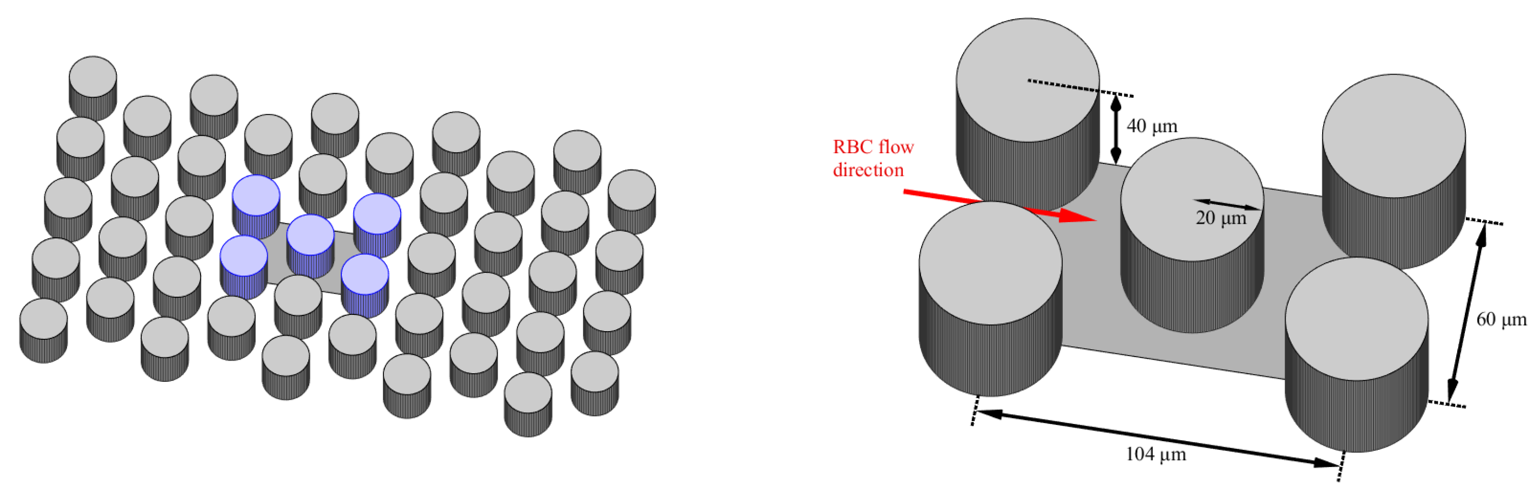
Figure 2.
Time series plot of ratio for a single healthy RBC.
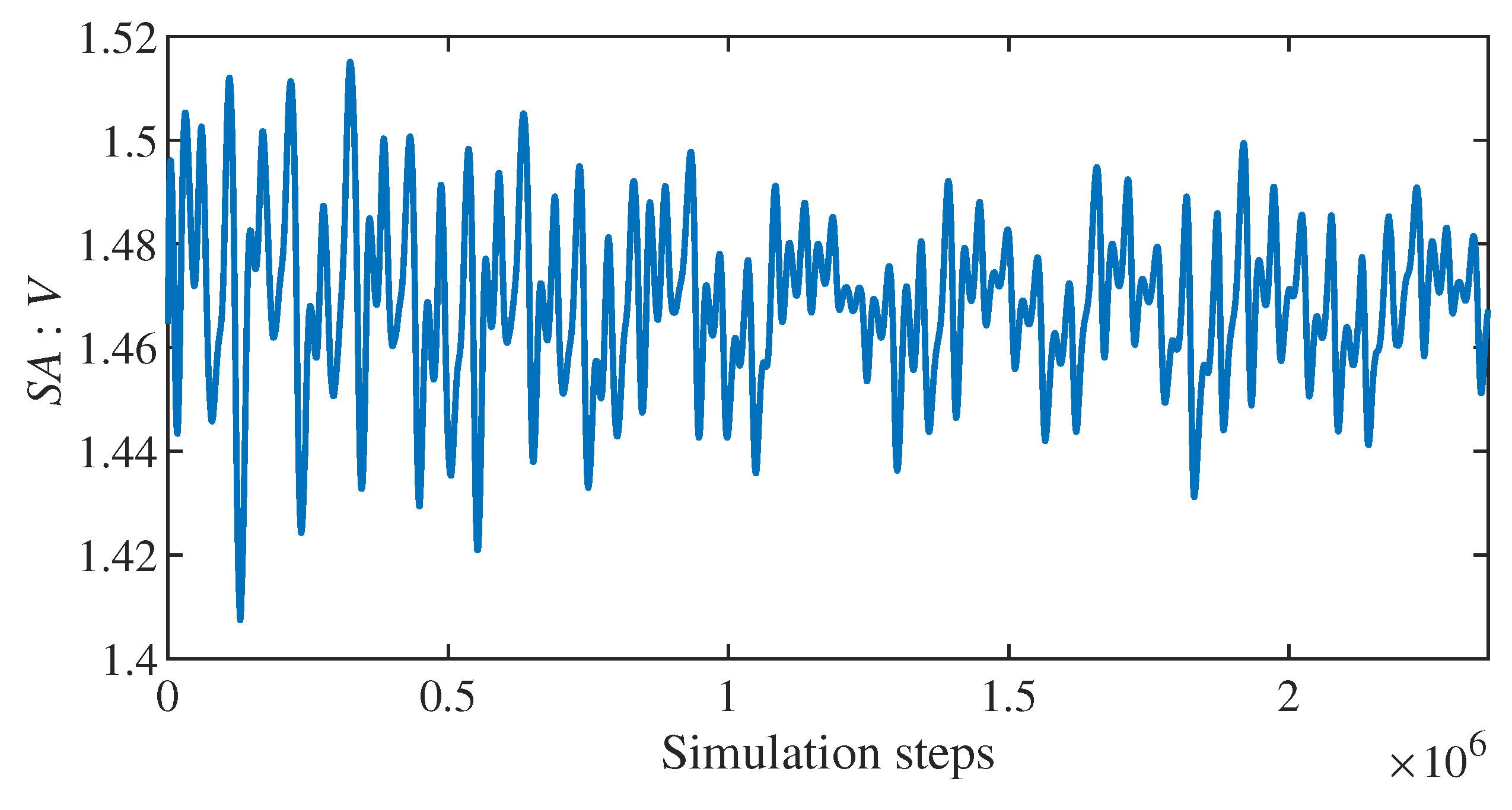
Figure 3.
Minimum, maximum and average ratio for nine healthy RBCs. Cells are sorted by average.
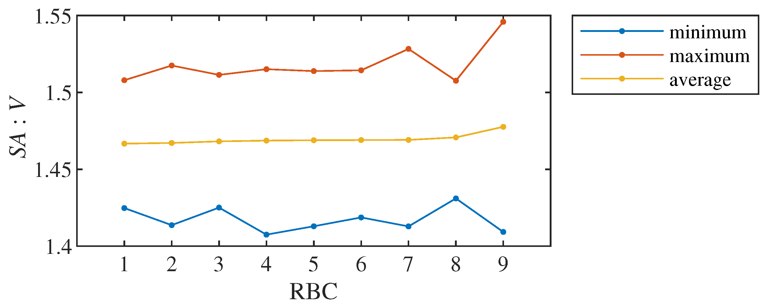
Figure 4.
Average, minimum, maximum and variance of ratio for all 4 cell types. Cells of each type are sorted by the observed characteristic for each plot.
Figure 4.
Average, minimum, maximum and variance of ratio for all 4 cell types. Cells of each type are sorted by the observed characteristic for each plot.
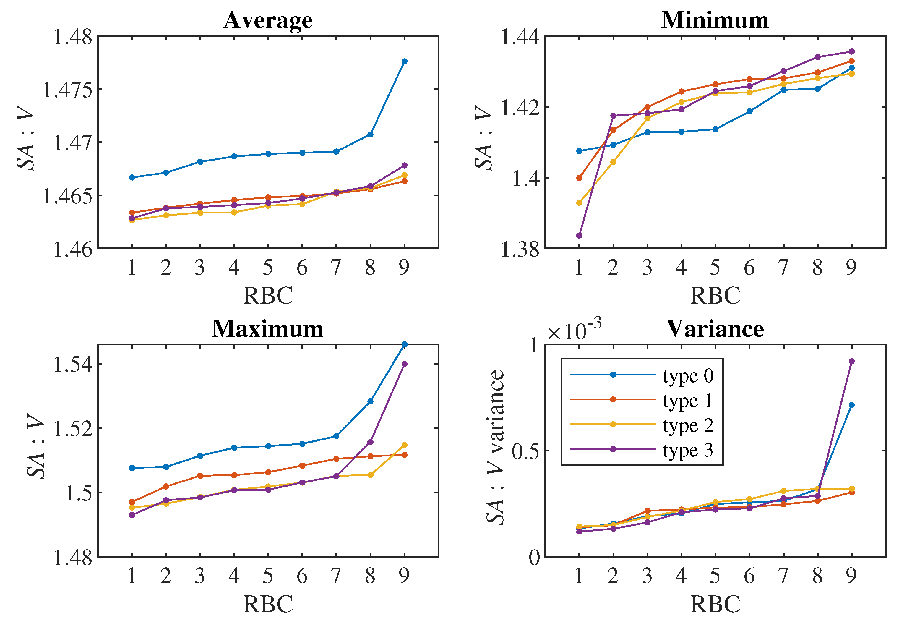
Figure 5.
Variance of surface area and volume for cell types 0 and 3.
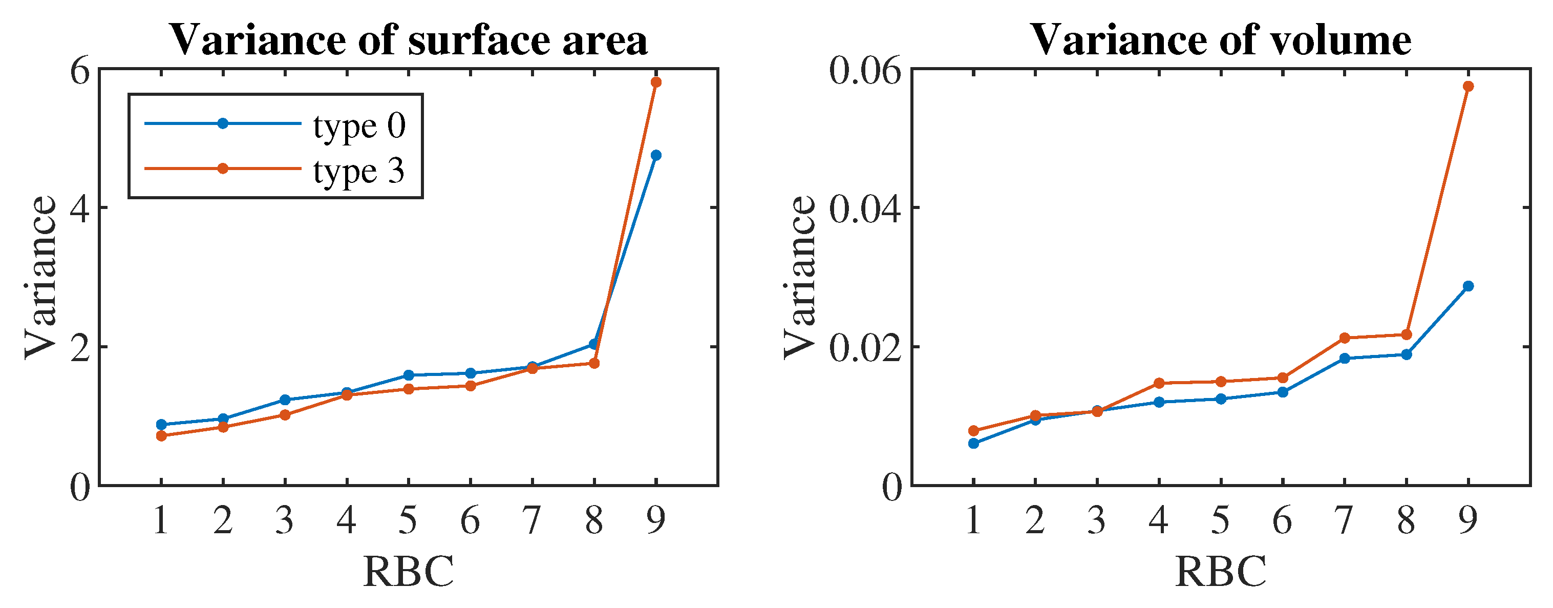
Figure 6.
Dependence of classification results on S when predicting 4 classes.
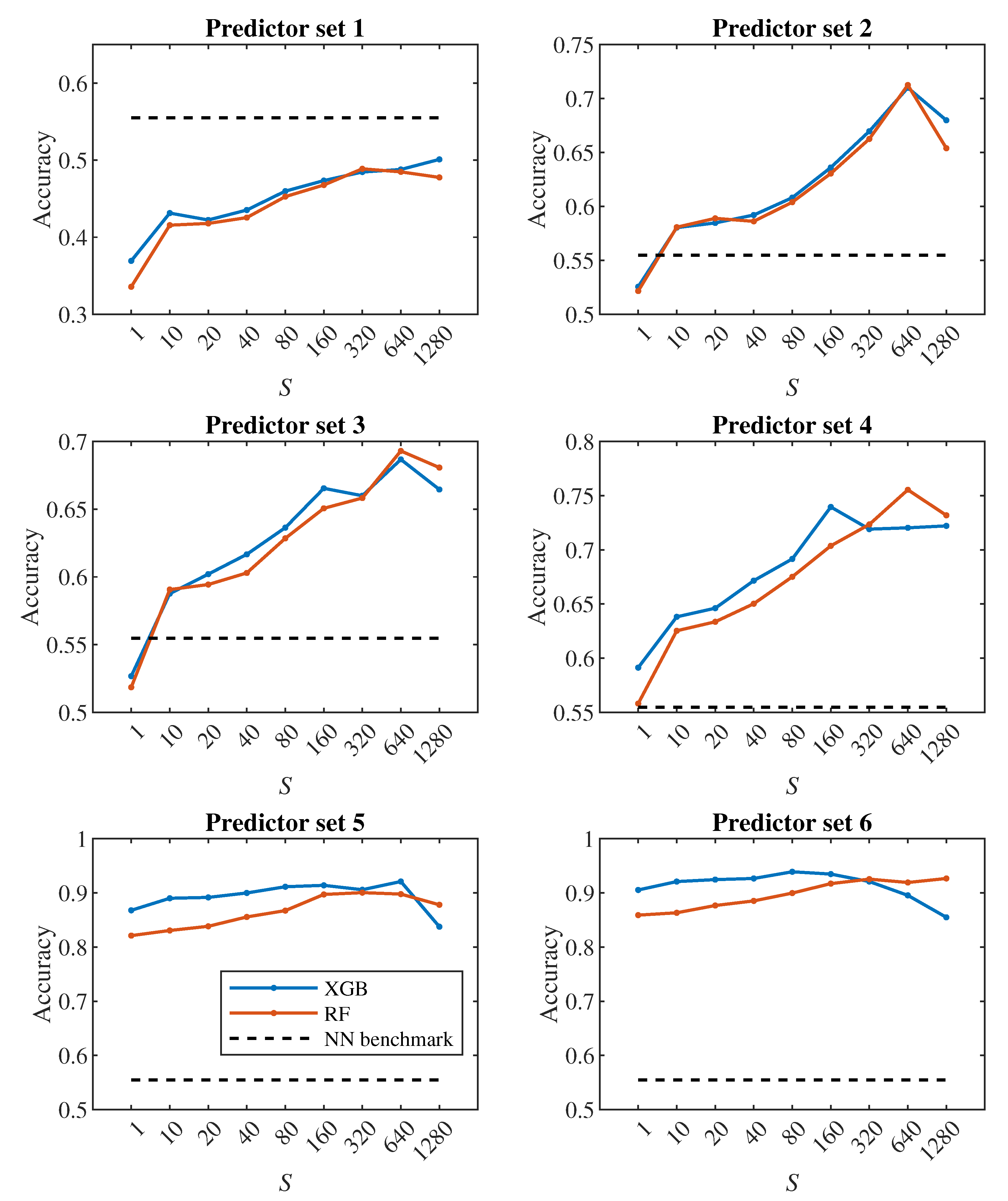
Figure 7.
Dependence of classification results on S when predicting 2 classes.
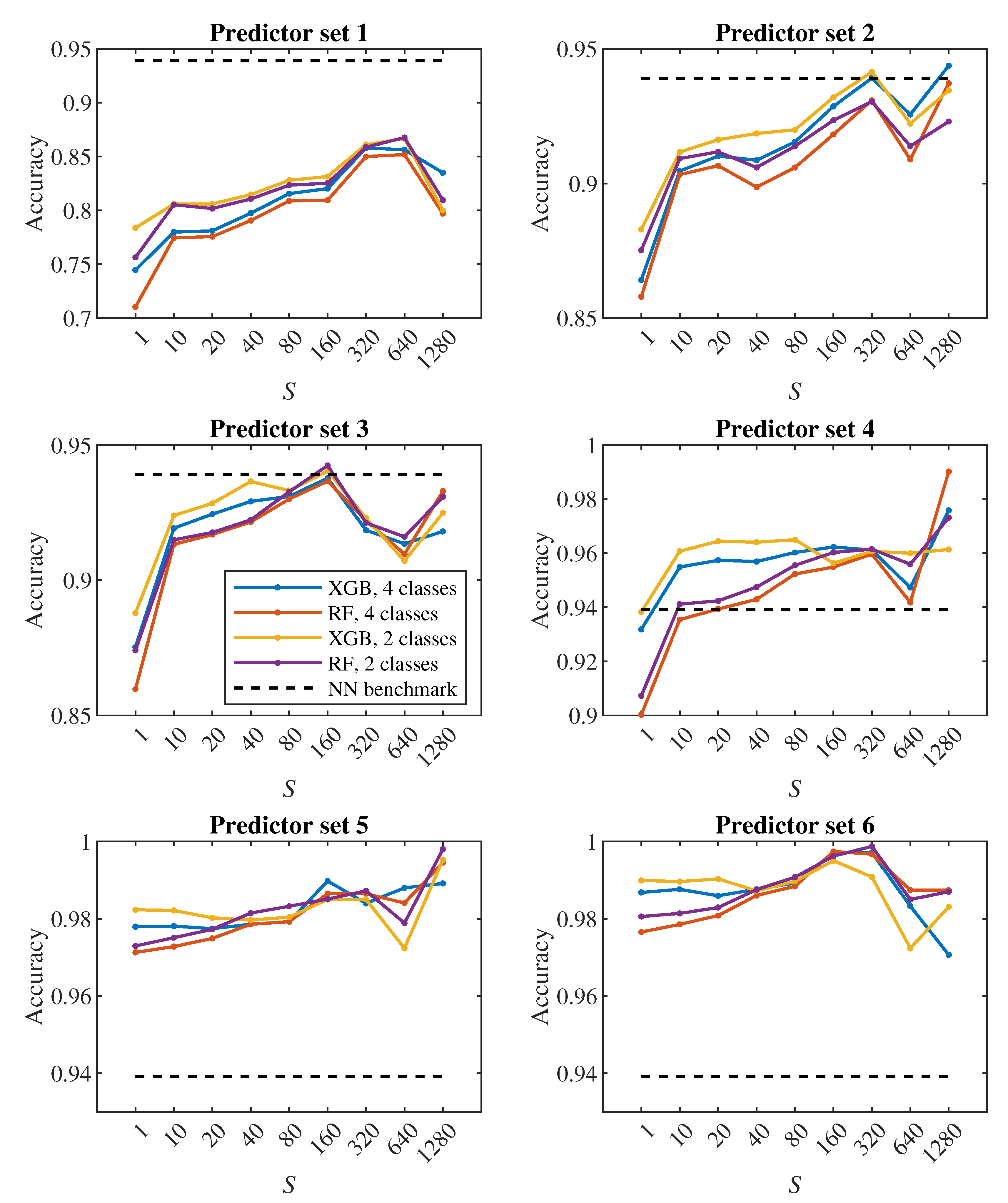
Figure 8.
Dependence of classification results on predictor set when predicting 4 classes.
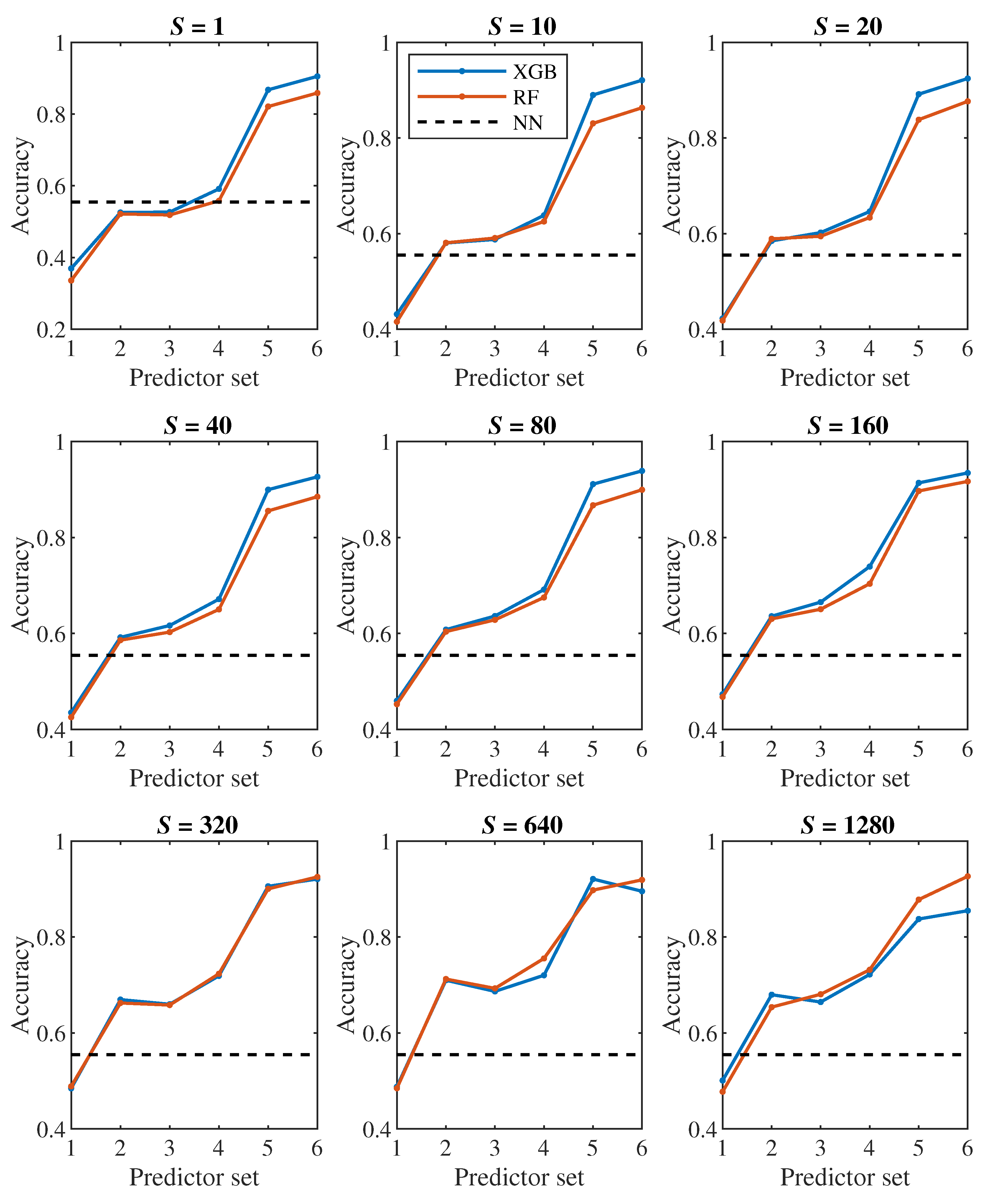
Figure 9.
Dependence of classification results on predictor set when predicting 2 classes.
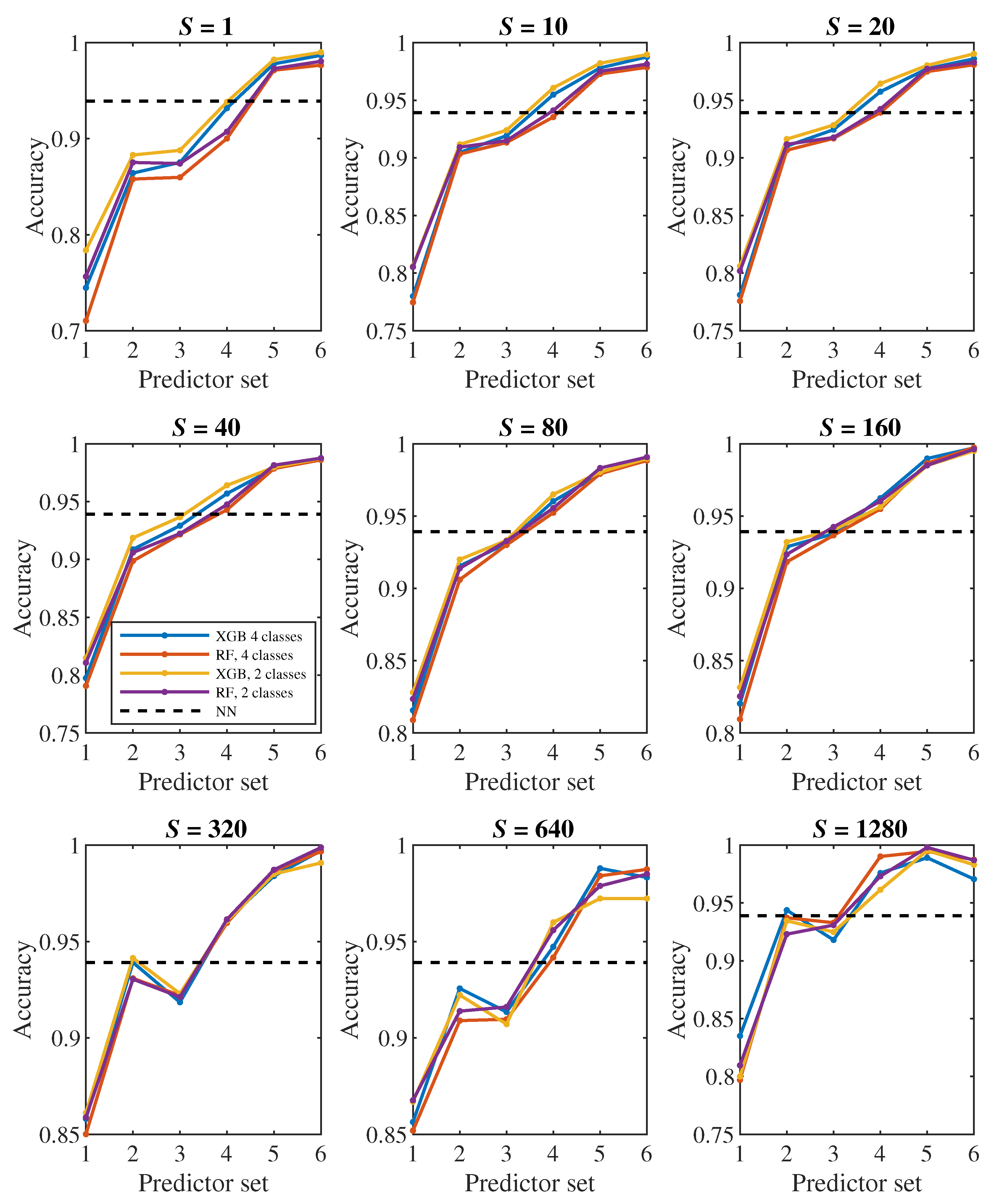
Figure 10.
Importance of predictors from the 6th set.
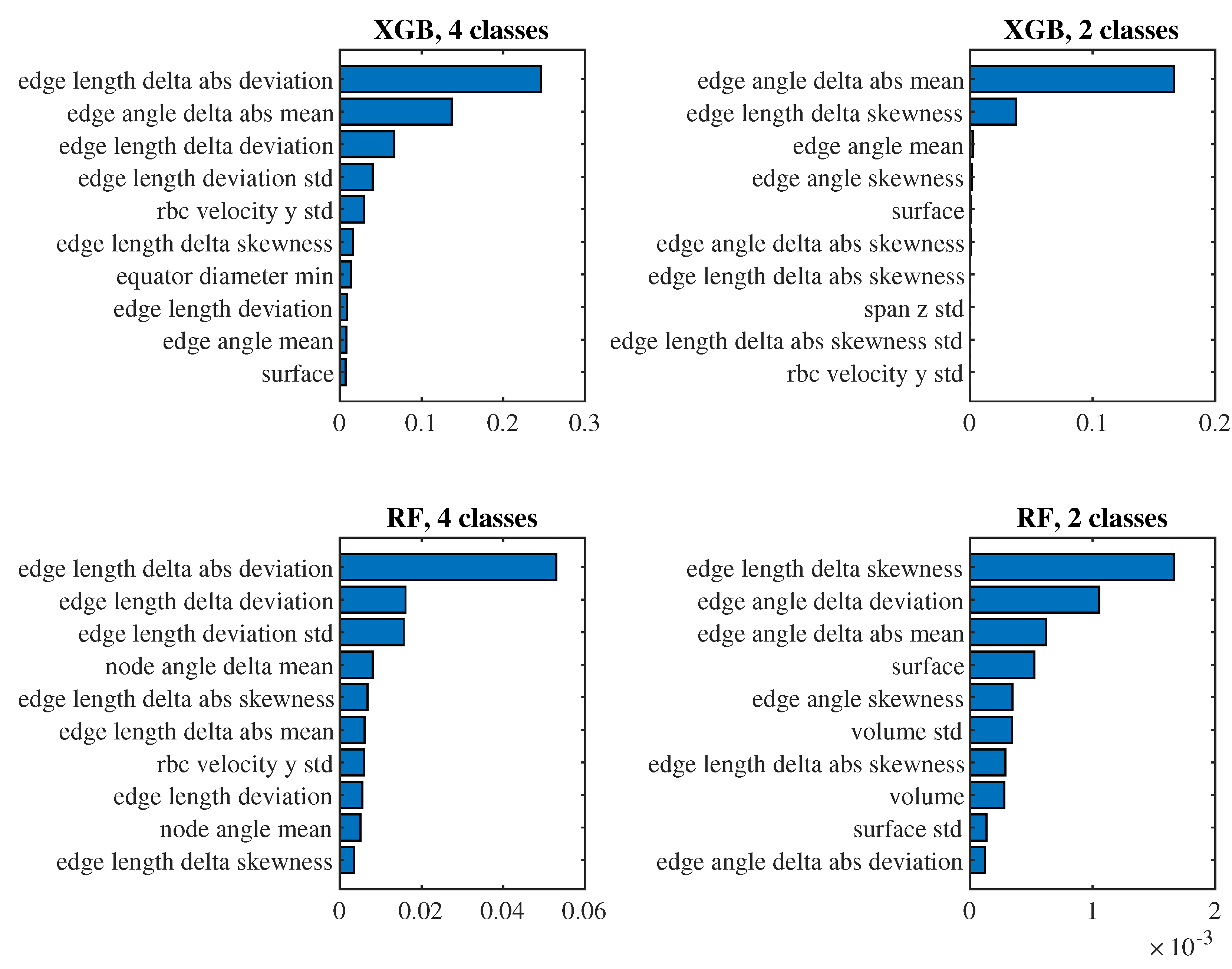
Figure 11.
Importance of predictors from the 4th set.
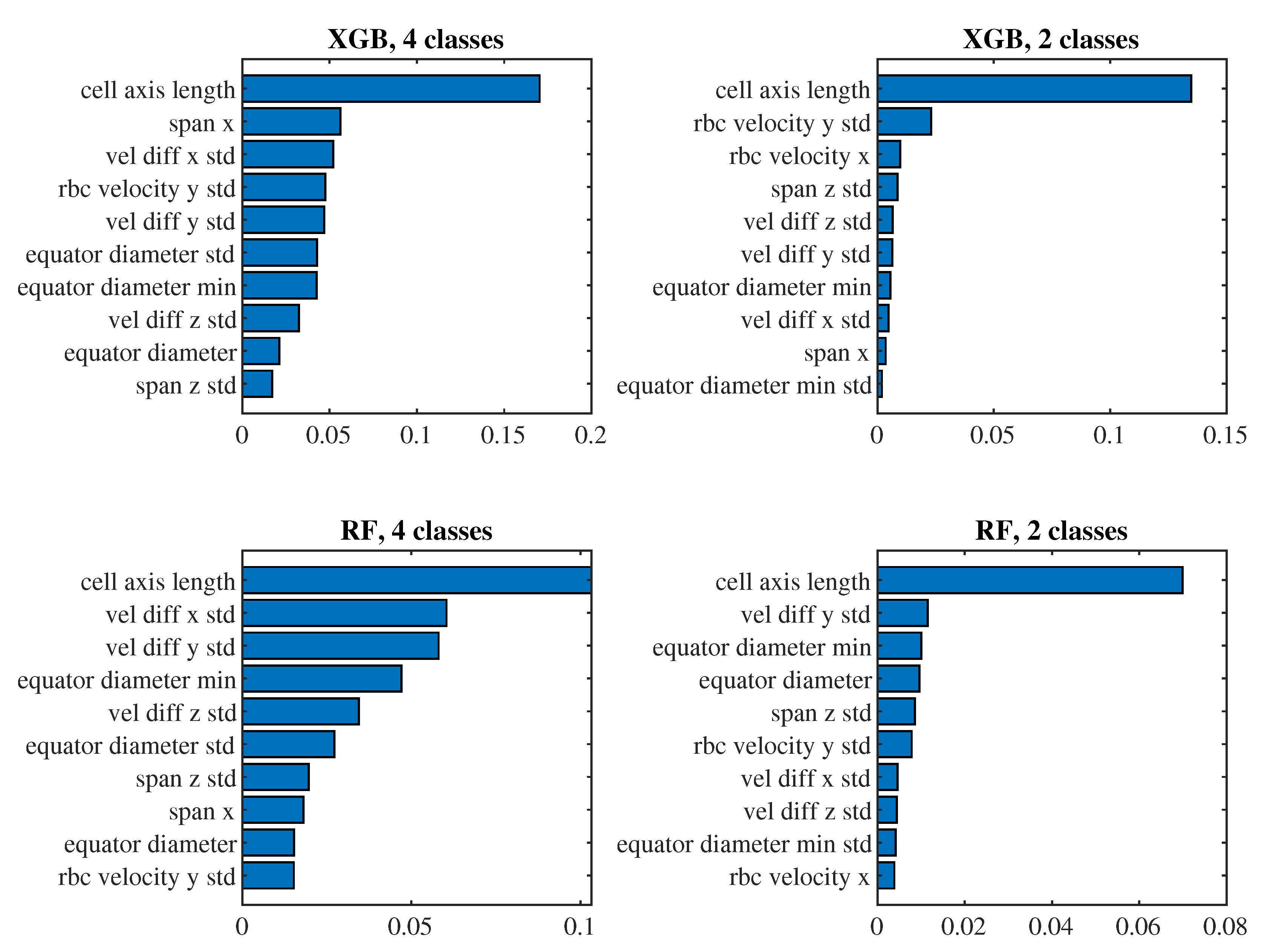

Table 1.
Elastic coefficients of the healthy RBC used in simulations.
| Parameter | Value |
|---|---|
| stretching coefficient () | 5 × 10⁻⁶ N/m |
| bending coefficient () | 3 × 10⁻¹⁹ N.m |
| coefficient of local area conservation () | 2 × 10⁻⁵ N/m |
| coefficient of global area conservation () | 7 × 10⁻⁴ N/m |
| coefficient of volume conservation () | 900N/m2 |
Table 2.
Results obtained by neural networks with EfficientNet_v2_B0 as the core model.
| Training number of classes | Validation and testing number of classes | Accuracy |
|---|---|---|
| 4 | 4 | 55.48% |
| 2 | 2 | 61.72% |
| 4 | 2 | 93.91% |
Table 3.
KS test results for average of .
| p-value | type 0 | type 1 | type 2 | type 3 | |
| D-value | |||||
| type 0 | 0 | 0.0007 | 0.0007 | ||
| type 1 | 1 | 0.3517 | 0.9895 | ||
| type 2 | 0.8889 | 0.4444 | 0.7301 | ||
| type 3 | 0.8889 | 0.2222 | 0.3333 | ||
Table 4.
KS test results for minimum of .
| p-value | type 0 | type 1 | type 2 | type 3 | |
| D-value | |||||
| type 0 | 0.3517 | 0.7301 | 0.3517 | ||
| type 1 | 0.4444 | 0.7301 | 0.9895 | ||
| type 2 | 0.3333 | 0.3333 | 0.7301 | ||
| type 3 | 0.4444 | 0.2222 | 0.3333 | ||
Table 5.
KS test results for maximum of .
| p-value | type 0 | type 1 | type 2 | type 3 | |
| D-value | |||||
| type 0 | 0.0336 | 0 | 0.0063 | ||
| type 1 | 0.6667 | 0.1256 | 0.1259 | ||
| type 2 | 1 | 0.5556 | 0.9895 | ||
| type 3 | 0.7778 | 0.5556 | 0.2222 | ||
Table 6.
KS test results for variance of .
| p-value | type 0 | type 1 | type 2 | type 3 | |
| D-value | |||||
| type 0 | 0.7301 | 0.9895 | 0.9895 | ||
| type 1 | 0.3333 | 0.7301 | 0.9895 | ||
| type 2 | 0.2222 | 0.3333 | 0.9895 | ||
| type 3 | 0.2222 | 0.2222 | 0.2222 | ||
Disclaimer/Publisher’s Note: The statements, opinions and data contained in all publications are solely those of the individual author(s) and contributor(s) and not of MDPI and/or the editor(s). MDPI and/or the editor(s) disclaim responsibility for any injury to people or property resulting from any ideas, methods, instructions or products referred to in the content. |
© 2024 by the authors. Licensee MDPI, Basel, Switzerland. This article is an open access article distributed under the terms and conditions of the Creative Commons Attribution (CC BY) license (http://creativecommons.org/licenses/by/4.0/).
Copyright: This open access article is published under a Creative Commons CC BY 4.0 license, which permit the free download, distribution, and reuse, provided that the author and preprint are cited in any reuse.


