Submitted:
20 August 2024
Posted:
20 August 2024
You are already at the latest version
Abstract
When earthquake damage occurs, it is extremely important to quickly identify the presence or absence of such damage. In this study, we developed and evaluated a new remote sensing index to automatically determine "damage" by image analysis when damage greater than partial destruction of a house by an earthquake or tsunami occurs. The accuracy of the houses estimated as "damaged" was high and sufficient for the initial assessment of damage. The results of this research are expected to be utilized for more rapid damage assessment after a disaster.
Keywords:
Earthquake
; Remote sensing
; House damage
1. Introduction
1.1. Assessing and Evaluating Damage at the Time of House Collapse by Earthquake
After an earthquake or a tsunami as a secondary disaster, it is common practice to remotely assess the damage from the sky by analyzing images using satellite imagery or UAVs with remote sensing technology. On the other hand, one of the problems with satellite images and UAV images is that it is difficult to accurately assess the situation depending on the weather conditions, resolution, and range of the images taken. In addition, 3D imagery and anomaly detection require sophisticated software, which is neither time- nor cost-effective for disaster sites [1,2,3,4,5]. One method to solve this problem is to enter the disaster site and capture video images while driving from a vehicle to quickly identify damaged areas [6]. The most common method for quickly capturing damage locations is to use a drive recorder, digital camera, or smartphone camera in order to maintain high image resolution and its accuracy. The most important task required in fieldwork is to quickly capture images and share the situation as quickly as possible, in addition to increasing their accuracy.
1.2. Disaster Recovery Processing Using Images
There have been many precedents for disaster recovery processing using images. For example, at the time of the Noto Peninsula earthquake in 2024, the National Research Institute for Earth Science and Disaster Prevention (NIED) published images of the disaster-stricken area taken by the Iwane Laboratories, LTD using a 360-degree camera on a car on bosaixview [7]. In addition, with the development of search engines such as Google and SNS such as X, images and videos are becoming big data. In the case of the Taiwan earthquake in April 2024 [8], images of the earthquake were shared on X and other social networking services. As the volume of information continues to expand, society will increasingly require the removal of unnecessary information, the extraction of accurate information only, and the prompt sharing of information when disasters occur [9,10,11,12].
1.3. Generation of New Indicator DI (Disaster Index) for Visible Remote Sensing
The colors we see in the human eye consist of spectral reflectance characteristics in the visible spectrum, and what we perceive as visual information is based on the reflectance intensity of red, blue, and green wavelengths, and we ascertain the color information of an object by these wavelengths. For example, we perceive vegetation as green because the intensity of green reflection is stronger than the intensity of red or blue reflection. Research is underway to apply these material properties to create indicators for remote sensing in the visible range. An equation that applies the fact that vegetation has high green reflectance and low red reflectance has been used as a vegetation indicator called VARI [13]. The chlorophyll-a concentration in water is also known as VWRI [14,15]. The reflectance for each physical property is shown in Figure 1. We attempted to generate a new indicator DI with reference to these spectral reflectance properties.
2. Methods
2.1. Flow Charts
The overall flow for satisfying the "with damage" requirement is shown in Figure 2. The details are explained step by step.
2.2. Generation of Disaster Index (DI)
The DI (Disaster Index) was generated by applying the difference in reflectance intensity. Since soil and wood have large red reflectance and small green reflectance, the DI was set up as in Equation (3). it is hypothesized that the DI can capture wood and soil runoff generated by house collapses and other disasters by their spectral reflectance characteristics, and its accuracy and utility are evaluated in this paper.
Calculate the DI in the image by calculating the Disaster Scale Index DI in Equation (3) for each pixel. The mean and standard deviation are calculated from the overall data of DI per pixel, and the values are used to determine "with damage" or "without damage. In this study, two methods are used to determine whether there is "damage" or "no damage": The first method calculates the average value of DI in an image to determine "damage"; the second method calculates the area of DI contained within a certain threshold value to determine "damage. In this paper, we compare these two methods to confirm their practicality.
- (1)
- Calculation method based on average values
The average value of DI for each image is calculated, and if the average value of DI for that image exceeds a certain threshold value, "Damage is present" is determined.
- (2)
- Calculation method based on the percentage of DI that meets certain conditions to the total area
In order to respond to the solar and weather conditions at the site, the disaster scale index DI for wood and sediment color was calibrated according to the site. The value used to calibrate the DI was used as DIcal, and if the pixel value of the target image was within the range from the average value of the DIcal to the value ασ away from it, then the pixel was considered to be a "damaged pixel". As shown in Equations (4) and (5), μ and σ are the mean and standard deviation of all pixels of the calibrated debris color (DIcal ). Also, α indicates an arbitrary number. The image used for calibration in this paper is shown in Figure 3. This image can be selected arbitrarily by the experimenter.
μ - ασ ≤ DI ≤ μ + ασ (α is an arbitrary number)
μ = average(DIcal ), σ = standard deviation(DIcal )
2.3. How to Divide the Area When Calculating DI
As shown in Figure 4, in images taken from the roadway, the upper half, i.e., in the areas (1) and (2) in the image, points to the distance or sky. Therefore, it is conceivable that the upper half may be removed when photographing the vicinity. By dividing the image into the lower left and right halves, i.e., (3) and (4), we decided to consider the image as a "damaged image" if the DI had a significant impact on one of the left and right halves. This is to ensure accurate judgment when comparing an image in which a house has collapsed on only one side and an image in which a house has collapsed on both sides. This delimitation method was applied in both the calculation method by average and by area.
3. Results
The authors attempted to estimate the scale of damage based on two methods using DI: the first method calculates the average value of DI for each image and determines "damage exists" when the average value of DI for that image exceeds a certain threshold value; the second method determines "damage exists" when the ratio of DI that meets certain conditions to the total area The second method is to judge "damage exists" when the ratio of DIs meeting certain conditions to the total area exceeds a certain threshold value. As a result, the following three differences were found to occur between the judgment method based on the average value of DI and the method based on the percentage of DI area after calibration. (1) accurate estimation of the scale of damage, (2) automation of threshold values, and (3) durability against misidentification of damage conditions.
3.1. Accurate Estimation of the Scale of Damage
No criteria exist for evaluating the scale of damage by the average value per pixel of the DI. Therefore, to solve this, calibration of the DI is a prerequisite; as indicated in the methodology, photographs of runoff sediment and timber for that land/weather condition were used to calibrate the DI. This allows for standardization of the scale of damage for that soil/weather condition. The "damaged" pixels (A) were determined to be "damaged" pixels if the DI value was close to the calibrated image, and "undamaged" pixels (B) if it was far away, in relation to the overall percentage, and the percentage of "damaged" pixels (A) in the total number of pixels (A+B) was calculated to The scale of damage was determined by calculating the percentage of "damaged" pixels (A) in the total number of pixels (A+B). This enabled the scale of damage to be calculated with high accuracy and quantitative values to be shown. For example, in the image shown in Figure 5 before calibration, it is necessary to show the partially damaged part of the house on the right, but it was not calculated well. On the other hand, in the post-calibration image, the percentage of "damaged pixels" to the area of the lower left portion is 0.001 (0.1%), and the percentage of "damaged pixels" to the area of the lower right portion is 0.087 (8.7%), indicating quantitative criteria, and the accuracy of "damaged The accuracy of the "damaged pixels" is also high.
3.2. Automated Thresholds
In setting the threshold value using the average of the DI, there is a need to manually determine it. On the other hand, when the threshold is set arbitrarily, manual determination would lead to spending a significant amount of time in calculating the scale of damage. On the other hand, when calculating by the percentage of the DI area after calibration, it is possible to automate the process by using the mean and standard deviation. Specifically, the DI value is set to an area that is within α times the mean (μ) to standard deviation (σ) of the pixel values in the image used for calibration. Here, α is an arbitrary value determined by the experimenter. Here, the ratio of the area to α is determined according to the standard normal distribution table. For example, if α is 1, the percentage of DI is set to 68% according to the standard normal distribution table. However, the authors found that setting the value of α to 0.1-0.3 optimizes the range the most.
3.3. Durability against Misidentification of Damage
In calculations using DI averages, the problem was that there were many cases of misrecognition of damage conditions. Even if the accuracy of recognition is improved by calibration, there are still cases of misrecognition. For example, the case shown in Figure 6. The car on the lower left is red, resulting in misrecognition by the DI. On the other hand, the indicator that was calibrated and showed a percentage of the total area could be correctly recognized as "no damage," although it was recognized.
As shown in 3.1-3.3, calibration with local images proved to be important in deriving the optimal solution.
4. Discussion
4.1. Further Improvement of Accuracy through Decentralization
At the stage of classifying images into those with damage and those without damage, there were several places where "no damage" images were misidentified as "damage" images. For example, it was found that they reacted to the red color of the car and the color of the soil being dug up. The problem was solved by using dispersion, although manual setting of the threshold was necessary. Unlike natural driftwood and sediment, artificial car colors and dug-up soil do not have variance in color. Therefore, setting the dispersion criterion in addition to the DI criterion enables more precise criterion setting for the "damage image.
4.2. 0.1σ . and 8% Value Calculation
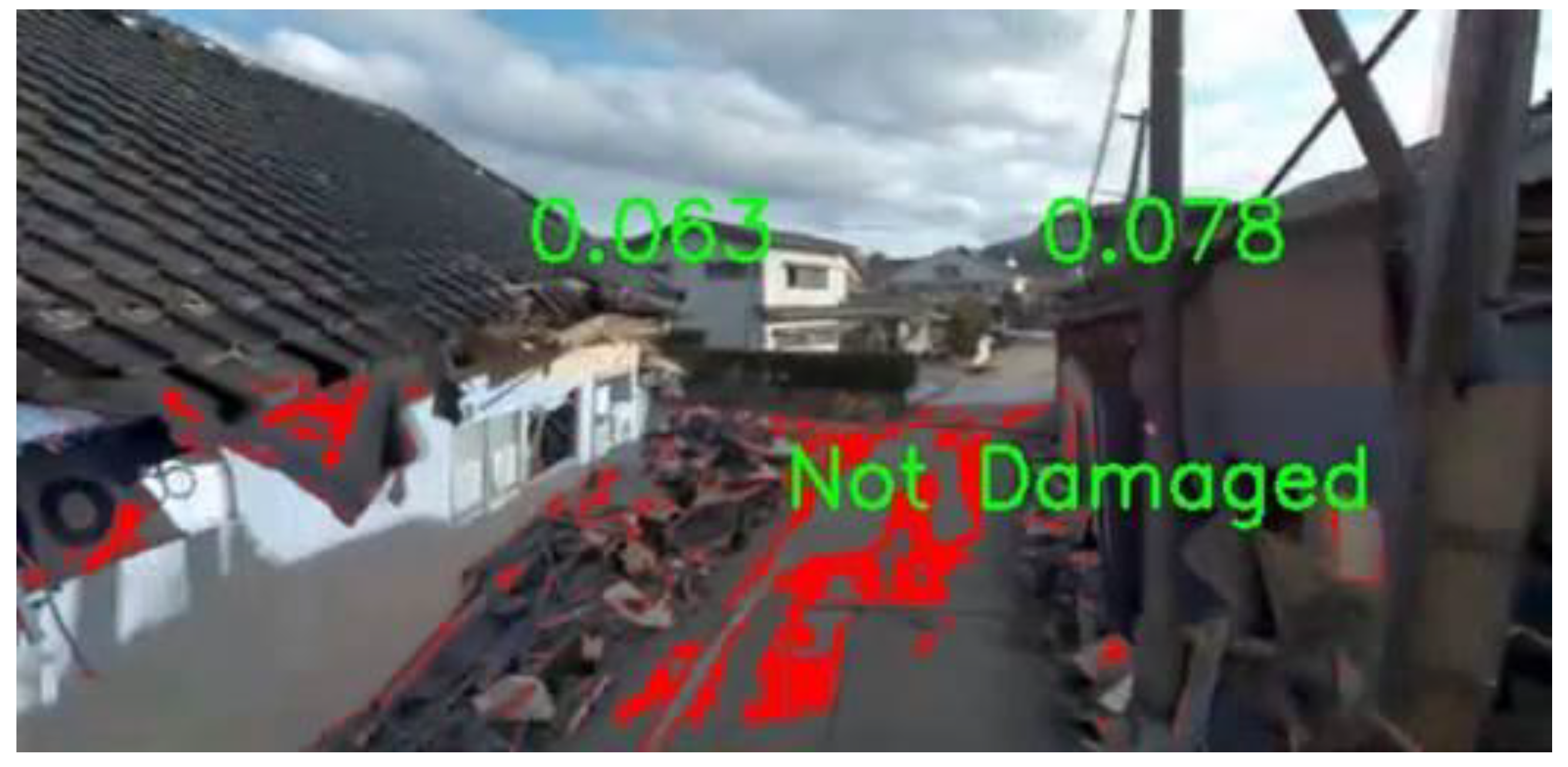
For the area from the calibrated rubble to the value that deviates by 0.1σ with DI to be 8% of the total area, the sum of the theoretical values of the bilateral percentages obtained by the normalized standard deviation table is adopted. σ is the standard deviation, so the color to be calibrated can be considered "damaged" as long as the solar radiation and weather conditions of the land are met. As long as the color to be calibrated satisfies the local solar and meteorological conditions, it can be considered "damaged. When an image of sediment completely unrelated to the affected area was used for calibration, the accuracy was found to be significantly lower, as shown in Figure 7. A value of 8% (0.08) or more is appropriate for a 0.1σ deviation, but if the color range is expanded to 0.2σ or 0.3σ, the value is calculated according to the coefficient of standard deviation using the normalized standard deviation table.
4.3. Accompanying Location Information and Mapping to Speed Up Damage Assessment
For example, by using the continuous-fire function of a smartphone camera to take pictures, multiple still pictures can be stored with the GPS information stored; by comparing the GPS information with the information on the presence or absence of damage in the pictures, it is possible to accurately inform the location of where the damage is located. In addition, the larger the area of DI, the more likely it is that the scale of damage is large, suggesting that quantitative map generation will also be possible. It is assumed that rapid assessment of the damage situation will lead to the sharing of information on the location and guide safe actions. In the initial response, it is important to determine how much human and property damage can be mitigated and how quickly information can be communicated. It is expected not only to estimate the amount of damage by quantitatively calculating the scale, but also to accurately convey "when," "where," and "what kind" of damage is occurring by promptly communicating the damage situation.
5. Conclusions
In this paper, emphasis is placed on how to quickly extract "damaged" information from image information at the scene of a disaster. This study differs from previous studies of other disasters in that it developed an image recognition index using only RGB, which minimizes the amount of computation, rather than machine learning or neural networks. This index can be used to qualitatively and quantitatively determine the scale of a disaster by calibrating it with images of the disaster site, and can be used not only to determine the scale of house collapses during an earthquake, but also to calculate the volume of sediment and driftwood. Ultimately, the authors intend to link it with location information and use it for participatory GIS and public and mutual aid. The authors hope that the use of this system will facilitate the understanding of post-disaster safety and damage in a more rapid manner.
Author Contributions
For research articles with several authors, a short paragraph specifying their individual contributions must be provided. The following statements should be used “Conceptualization, H.S and Y.U.; methodology, H.S.; software, H.S.; validation, H.S; formal analysis, H.S.; investigation, H.S and Y.U.; resources, Y.U.; data curation, Y.U.; writing—original draft preparation, H.S.; writing—review and editing, H.S.; visualization, H.S.; supervision, Y.U.; project administration, Y.U.; funding acquisition, H.S. All authors have read and agreed to the published version of the manuscript.
Funding
This work was supported by JST SPRING, Japan Grant Number JPMJSP2124.
Data Availability Statement
Not applicable.
Acknowledgments
Dr. Yoshinobu Mizui (REIC) provided advice on estimating disaster litter from photographs. We also thank Iwane Laboratories, LTD for advice on 3D analytical methods. We would like to express our gratitude to them, who supported us in the completion of this research. This work was supported by JST SPRING, Japan Grant Number JPMJSP2124. Dr. Yoshinobu Mizui (REIC) provided advice on estimating disaster litter from photographs. We also thank Iwane Laboratories, LTD for advice on 3D. We would like to express our gratitude to the many people who supported us in the completion of this research.
Conflicts of Interest
The authors declare no conflict of interest. The funders had no role in the design of the study; in the collection, analyses, or interpretation of data; in the writing of the manuscript; or in the decision to publish the results.
References
- Kanamori, Hiroo. Mechanism of tsunami earthquakes. Physics of the earth and planetary interiors 1972, 6, 346–359. [Google Scholar] [CrossRef]
- Okamoto, T. Takenaka, H., Nakamura, T. et al. FDM simulation of earthquakes off western Kyushu, Japan, using a land-ocean unified 3D Earth Planets. Space 2017, 69, 88. [Google Scholar] [CrossRef]
- Chen, Jinhong, et al. Damage degree evaluation of earthquake area using UAV aerial image. International Journal of Aerospace Engineering 2016, 1, 2052603.
- Voigt, Stefan, et al. Satellite image analysis for disaster and crisis-management support. IEEE transactions on geoscience and remote sensing 2007, 45, 1520–1528.
- Chandola, Varun, Arindam Banerjee, and Vipin Kumar. Anomaly detection: A survey. ACM computing surveys (CSUR) 2009, 41, 1–58.
- Mizui, Y Estimate the Amount of Disaster Waste Disposal Work Using In-Vehicle Camera Images - A Case Study in Hitoyoshi City, Kumamoto Prefecture - A Case Study in Hitoyoshi City, Kumamoto. Journal of Disaster Research 2021, 16, 1061–1073. [CrossRef]
- 2024 Noto earthquake bosaixview. Available online: https://xview.bosai.go.jp/view/index.html?appid=41a77b3dcf3846029206b86107877780 (accessed on June 2024).
- Kanwal, Maria, Assessing the Impact of the 2024 Hualien Earthquake in Taiwan (April 6, 2024). Available online: https://ssrn.com/abstract=4786199.
- Li, Xianju, et al. Identification of forested landslides using LiDar data, object-based image analysis, and machine learning algorithms. Remote sensing 2015, 7, 9705–9726.
- Anwar, Syed Muhammad, et al. Medical image analysis using convolutional neural networks: a review. Journal of medical systems 2018, 42, 1–13.
- Koskosidis, Y.A. Powell, W. B. and Solomon, M. M.: An Optimization-Based Heuristic for Vehicle Routing and Scheduling with Soft Time Window Constraints. Transportation Science 1992, 26, 69–85. [Google Scholar] [CrossRef]
- Taniguchi, E., Yamada, T. and Kakimoto, Y.: Probabilistic vehicle routing and scheduling with variable travel times. In Proceedings of the 9th IFAC Symposium Control in Transportation Systems 2000, Braunschweig, Germany, 13-15 June 2000.
- Gitelson, A.; et al. Vegetation and Soil Lines in Visible Spectral Space: A Concept and Technique for Remote Estimation of Vegetation Fraction. International Journal of Remote Sensing 2002, 23, 2537–2562. [Google Scholar] [CrossRef]
- Shiraishi, H. New Index for Estimation of Chlorophyll-a Concentration in Water with RGB Value. Int J Eng Technol 2018, 18, 10–16. [Google Scholar]
- Cobelo, I.; et al. Unmanned aerial vehicles and low-cost sensors as tools for monitoring freshwater chlorophyll-a in mesocosms with different. International Journal of Environmental Science and Technology 2023, 20, 5925–5936. [Google Scholar] [CrossRef]
- Available online: https://seos-project.eu/classification/classification-c01-p05.html.
Figure 1.
Wavelength rates by physical properties (water, vegetation, soil) [16].
Figure 1.
Wavelength rates by physical properties (water, vegetation, soil) [16].
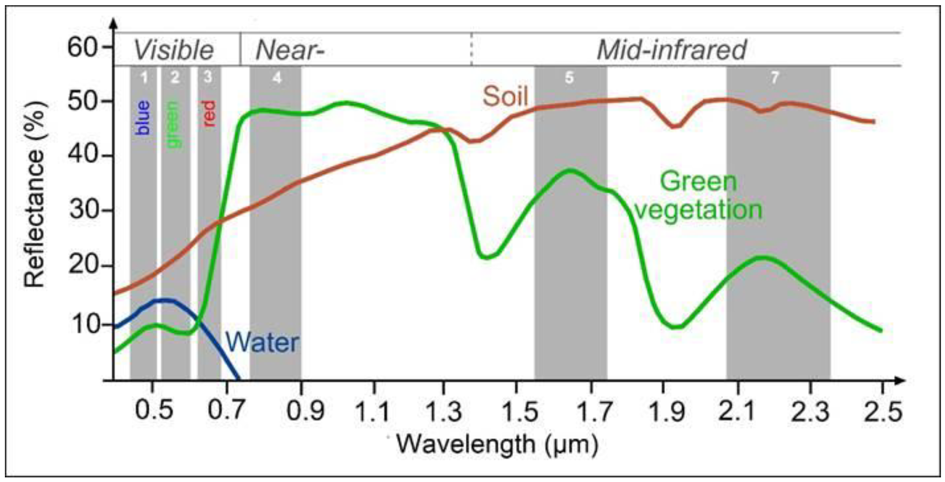
Figure 2.
Evaluation Criteria for DI that Satisfies the "Damaged" Criteria.
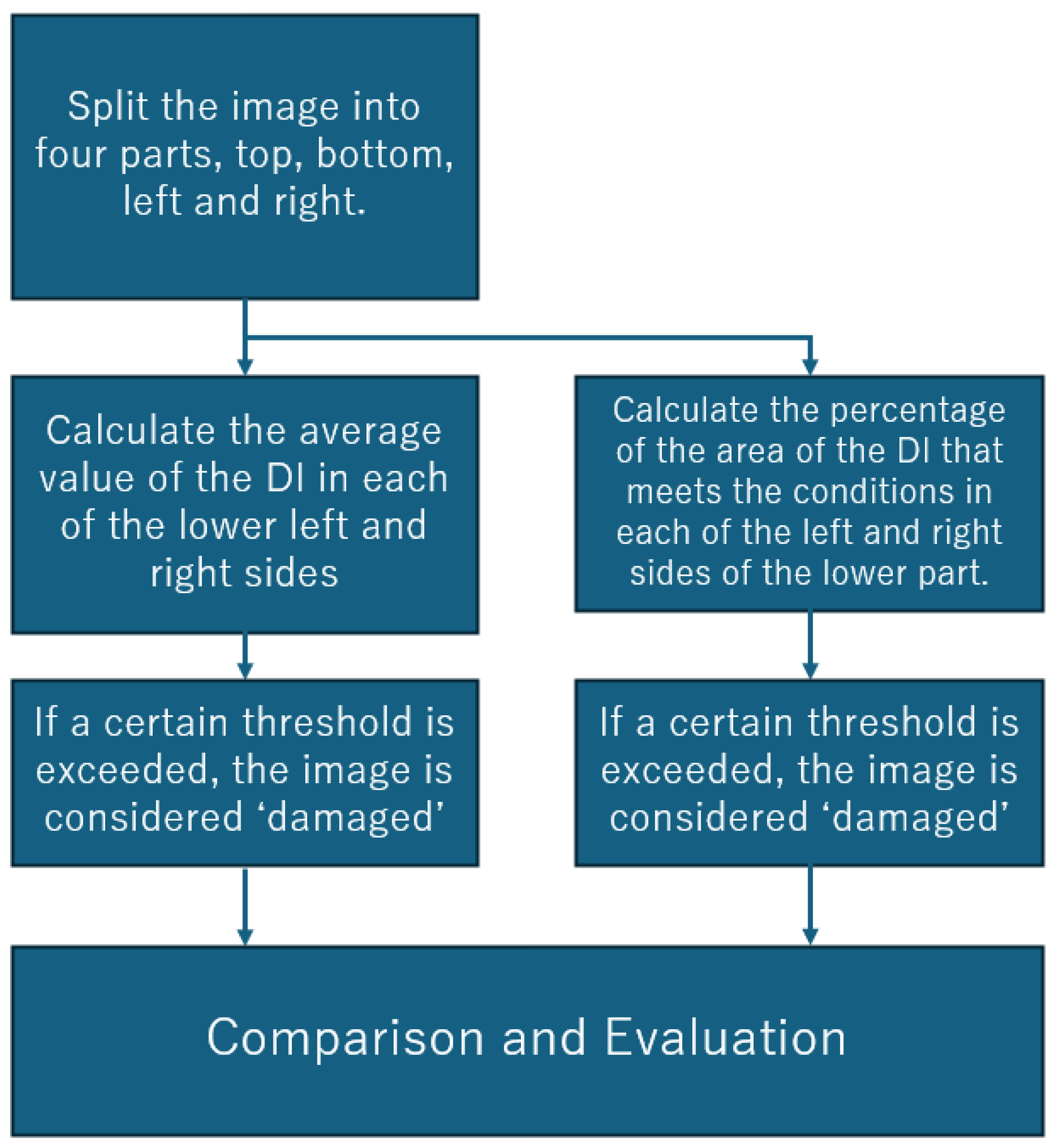
Figure 3.
Example of debris used for calibration.
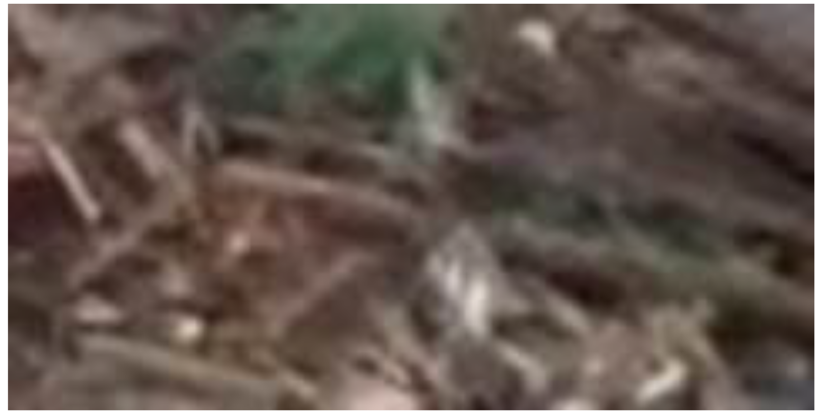
Figure 4.
Image of the affected area divided into top, bottom, left, and right.
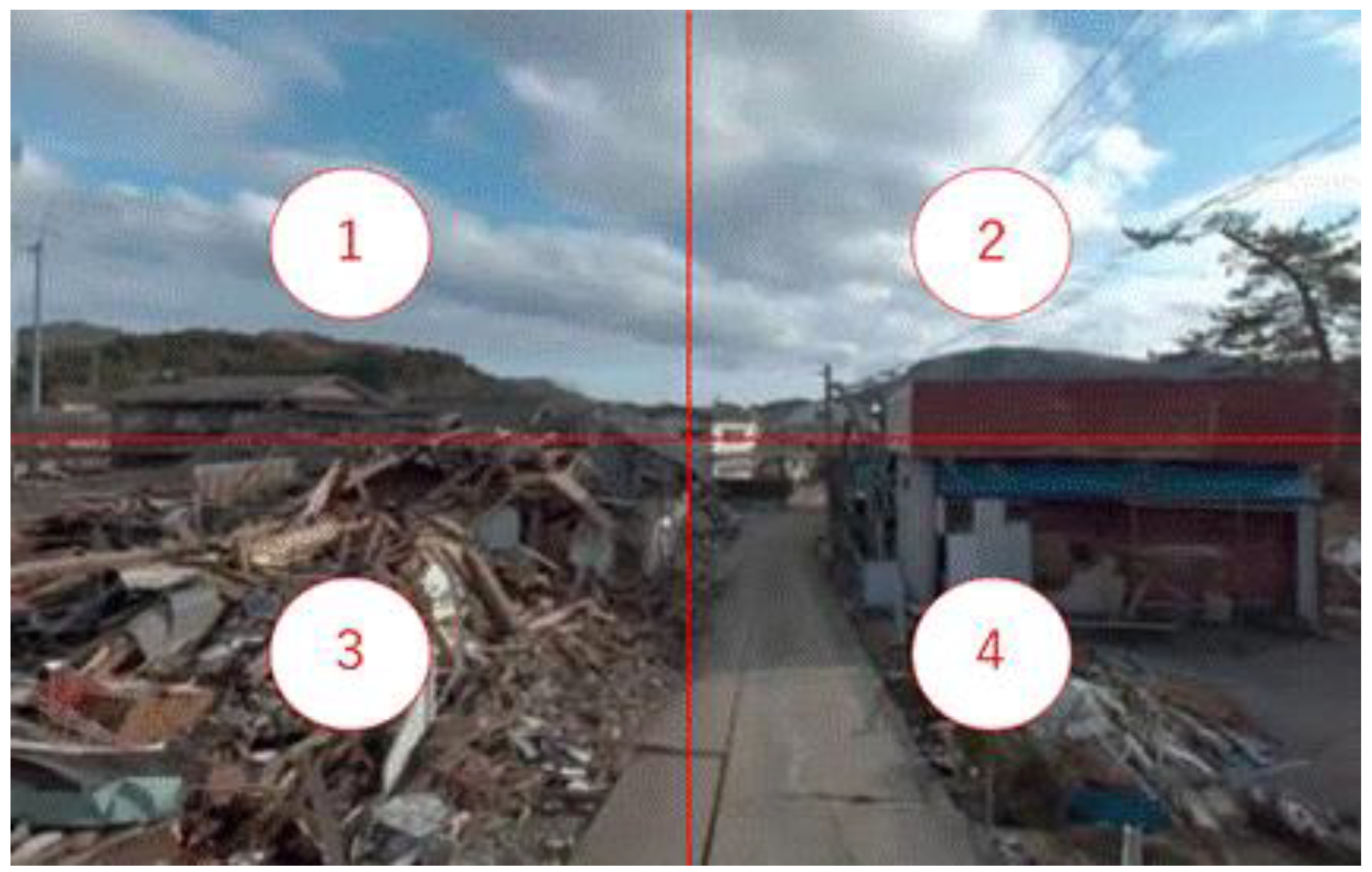
Figure 5.
(Top) Value calculated by the average of DI (The red area should indicate the area with the most damage, but in fact it is not shown correctly.) (Bottom) Image calculated by the percentage of DI area after calibration (The red area is the damaged area and is shown correctly. If the value exceeds a certain level, it is considered "damaged.).
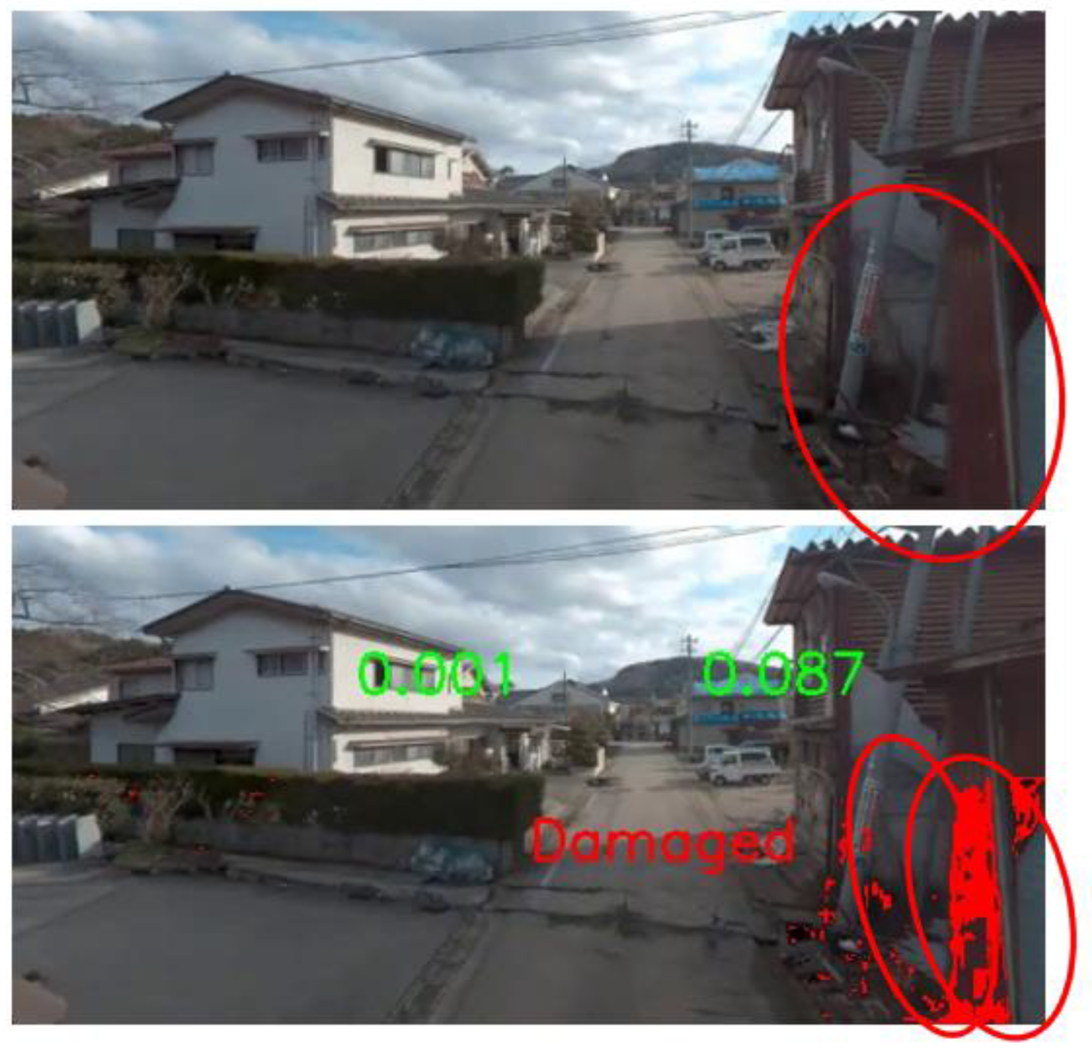
Figure 6.
(Top) Example of misidentification as "damaged" by the average of DI (Bottom) An example of correctly identifying "Not Damaged" by the percentage of DI area calibration (the soil in the lower left was misidentified but recognized as "Not Damaged" because it was a small percentage of the total area.).
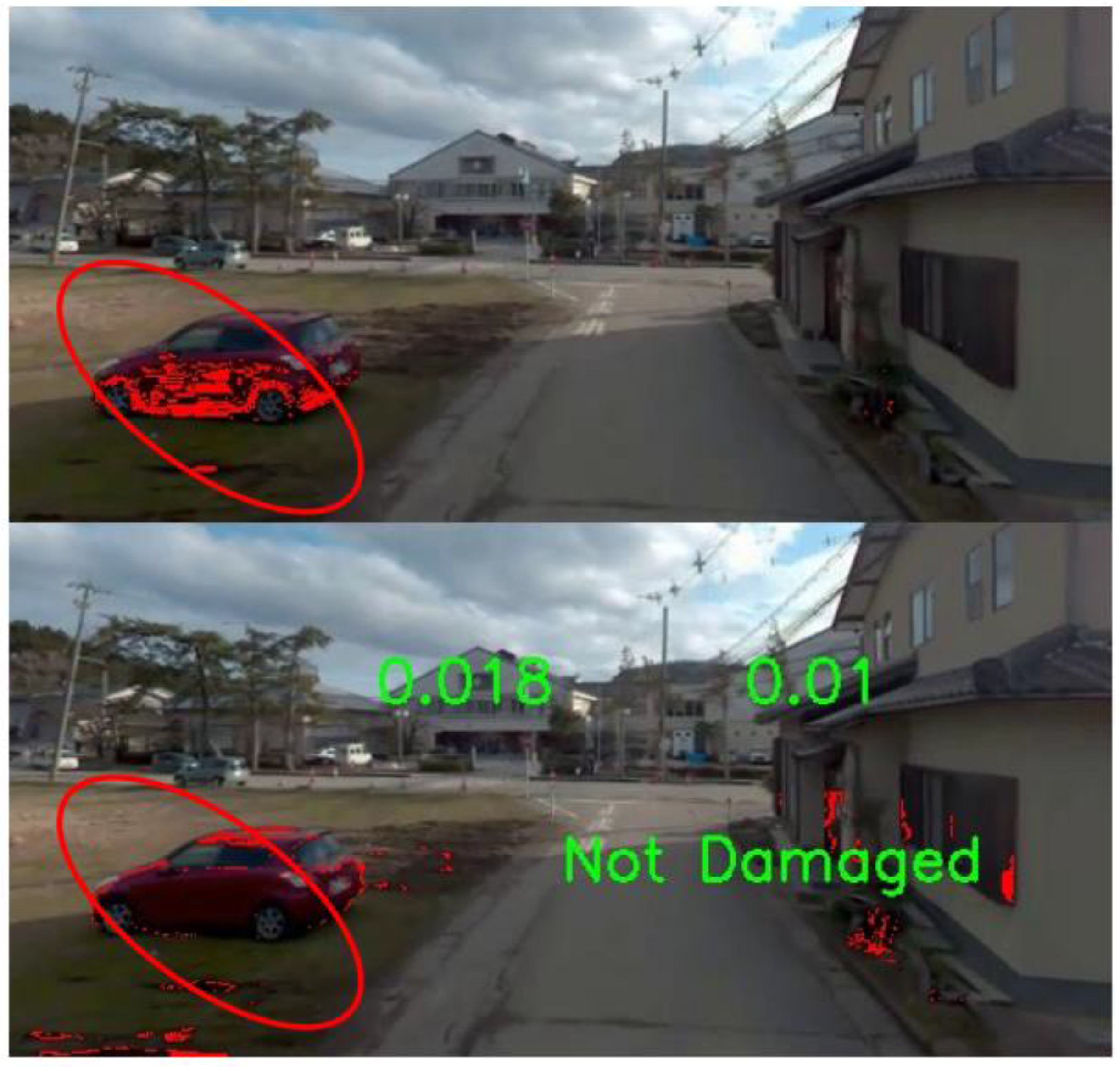
Figure 7.
Example of significant loss of accuracy when calibrating with unrelated images.
Disclaimer/Publisher’s Note: The statements, opinions and data contained in all publications are solely those of the individual author(s) and contributor(s) and not of MDPI and/or the editor(s). MDPI and/or the editor(s) disclaim responsibility for any injury to people or property resulting from any ideas, methods, instructions or products referred to in the content. |
© 2024 by the authors. Licensee MDPI, Basel, Switzerland. This article is an open access article distributed under the terms and conditions of the Creative Commons Attribution (CC BY) license (http://creativecommons.org/licenses/by/4.0/).
Copyright: This open access article is published under a Creative Commons CC BY 4.0 license, which permit the free download, distribution, and reuse, provided that the author and preprint are cited in any reuse.


