Submitted:
01 September 2024
Posted:
04 September 2024
You are already at the latest version
Abstract
The Riemann zeta function plays a crucial role in number theory and its applications. The Riemann Hypothesis (RH) posits that zeros of other than the trivial ones are located on the line defined by the equation Re(s) =1/2. This paper introduces a novel and straightforward proof of the Riemann Hypothesis. The proof employs a standard method, utilizing the eta function in place of the zeta function, under the assumption that the real part is greater than zero. The equation for the real and imaginary parts of the Riemann zeta function (eta function) is completely separated. Initially, let with s= . The value of the real part is determined by solving the equation, and the process is repeated for identifying the potential roots shared by the two functions, a common value is obtained, leading to a =1/2, which represents the real part of the main root of the function ζ(s). By plotting the zeta function for the obtained a, it is determined that the function has a root only at a =1/2. In another analysis, by identifying the roots of the common potential between the two functions ζ(s) and ζ(1-s), a common value is obtained, which leads to a =1/2. This value represents the real part of the main root of the function ζ(s). Additionally, using a standard method and with the help of two functions ζ(s) and ζ(1-s), the real part of the root of the zeta function is obtained. To create a generator function for prime numbers in terms of b, one can solve the root of the zeta function where it equals one (i.e., and obtain a relationship between b’ and prime numbers. Giving the value of zeta equal to one and s' = a' + ib’, similar to zeta equal to zero, the roots are again placed on the line. Then, by using the zeta function defined by multiplying prime numbers, we arrive at a new meaningful relation between b’ and its corresponding prime number is obtained.
Keywords:
Riemann Zeta Function
; Number Theory
; Riemann's Hypothesis
1. Introduction
The Riemann Zeta Function embodies both additive and multiplicative structures in a single function, making it the most important tool in the study of prime numbers. The Riemann zeta function is crucial in number theory and has applications in physics, probability theory, and applied statistics. It is named after the German mathematician Bernhard Riemann, who discussed it in the memoir "On the Number of Primes Less Than a Given Quantity," published in 1859.[1] Riemann knew that the function equals zero for all negative even integers -2,-4,-6, etc.(referred to as trivial zeros), and that it has an infinite number of zeros in the critical strip of complex numbers between the lines x = 0 and x = 1. Riemann conjectured that all nontrivial zeros are on the critical line, a conjecture that later became known as the Riemann hypothesis. In 1900, the German mathematician David Hilbert referred to the Riemann Hypothesis as one of the most important questions in all of mathematics, as evidenced by its inclusion in his influential list of 23 unsolved problems that he presented to 20th-century mathematicians. [2]
2. Riemann Hypothesis
The real part of every nontrivial zero of the Riemann zeta function is 1/2. Therefore, if the hypothesis is correct, all nontrivial zeros lie on the critical line consisting of the complex numbers ( b), where b is a real number and i is an imaginary unit.
2.1. Riemann Zeta Function
The Riemann zeta function can be expressed in the following form for complex s.ζ ( s ) = ∑ n = 1 ∞ 1 n s = 1 1 s + 1 2 s + 1 3 s + ⋯
The Riemann hypothesis discusses zeros outside the region of convergence of this series and Euler product. To make sense of the hypothesis, it is necessary to analytically continue the function to obtain a form that is valid for all complex s. Because the zeta function is meromorphic, all choices of how to perform this analytic continuation will lead to the same result, by the identity theorem. A first step in this continuation observes that the series for the zeta function and the Dirichlet eta function satisfy the relation within the region of convergence for both series.
However, the zeta function series on the right converges not just when the real part of s is greater than one, but more generally whenever s has a positive real part. Thus, the zeta function can be redefined as , extending it from Re(s) > 1 to a larger
domain: Re(s) > 0, except for the points where is zero.
In the strip 0 < Re(s) < 1 this extension of the zeta function satisfies the functional equation.
We start by converting relation 2 into a complex form.
By utilizing the trigonometric relationship, we can convert Riemann’s zeta function from a complex form to a sinusoidal form.
By using the following trigonometric relation and multiplying both equations 9 and 10 by cos (θ) and
sin(θ), then add them.
Relation 15 is considered a Reference Relation, so that every final relation will be compared with it in all stages of the proof.
In this way, we can write in complex form.
2.2. Proof of the Riemann Hypothesis
2.2.1. Determining the Value of “a” in
First, convert equation 9 from cosine to sine, and
then add equation 10 to obtain equation 27.
By expanding equation 27 using the trigonometric
relation, we obtain equation 28.
Divide both sides of equation 28 by
In the second sentence of relation 29, we make a small
change because 1 minus 1 equals 0.
With the use of 31, we will have.
Once we have defined the relationships, we can
revisit the Function, which is similar to relation #15.
If the expression- is equal to zero and the expression () is equal to one, then Equation 32 becomes similar
to Relation 15.
…+
To obtain a, the manipulation of function clauses
was only done in the second clause, which includes the prefix. The expression -1+1 is added to it, resulting in
a favorable outcome that confirms the correctness of Riemann's Hypothesis.
However, manipulating the remaining sentences yields new values for a, which
necessitates checking if there is a root on these new lines. We start from
equation 29.
If the expression equals to zero and the expression equals to one, then Relation 35 becomes similar to
Relation 15.
#
If the expression equals to zero and the expression equals to one, then Relation 37 becomes similar to
Relation 15.
Graphical Proof:
By plotting the function at certain points, it is easy to understand that the Zeta Riemann function has no roots at these points except for the Re(s) =
Figure 1.
Plots of | with
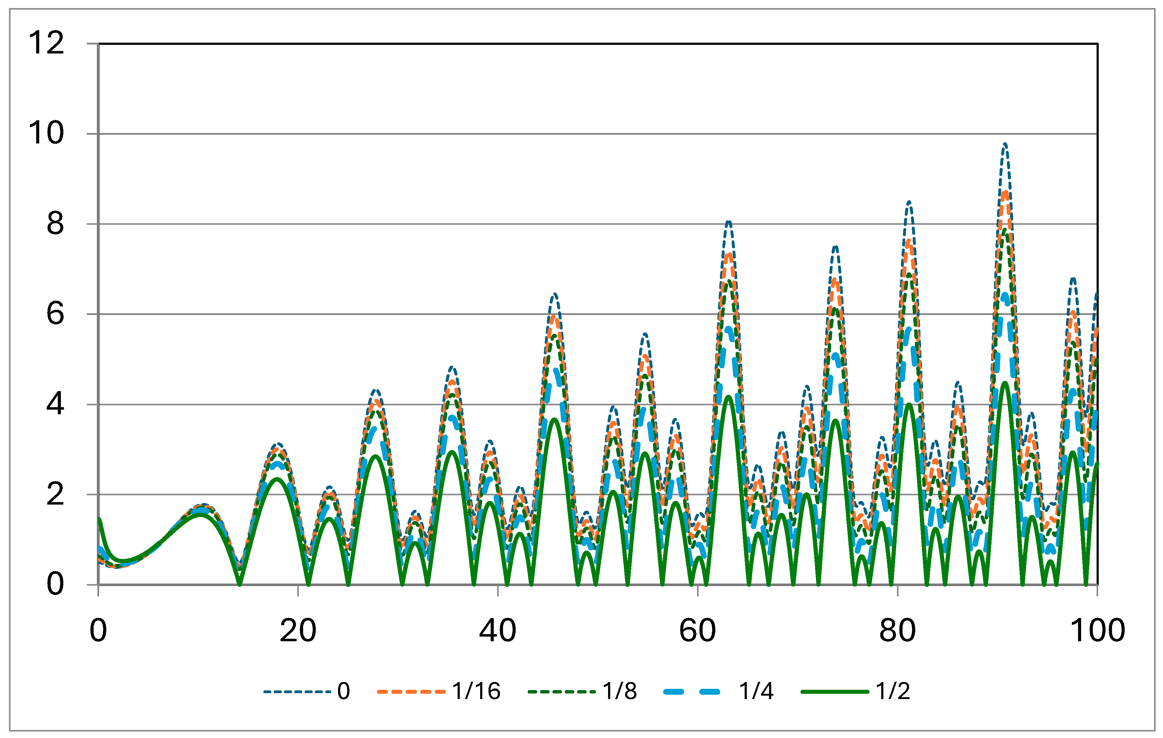
Figure 2.
Plots of | with
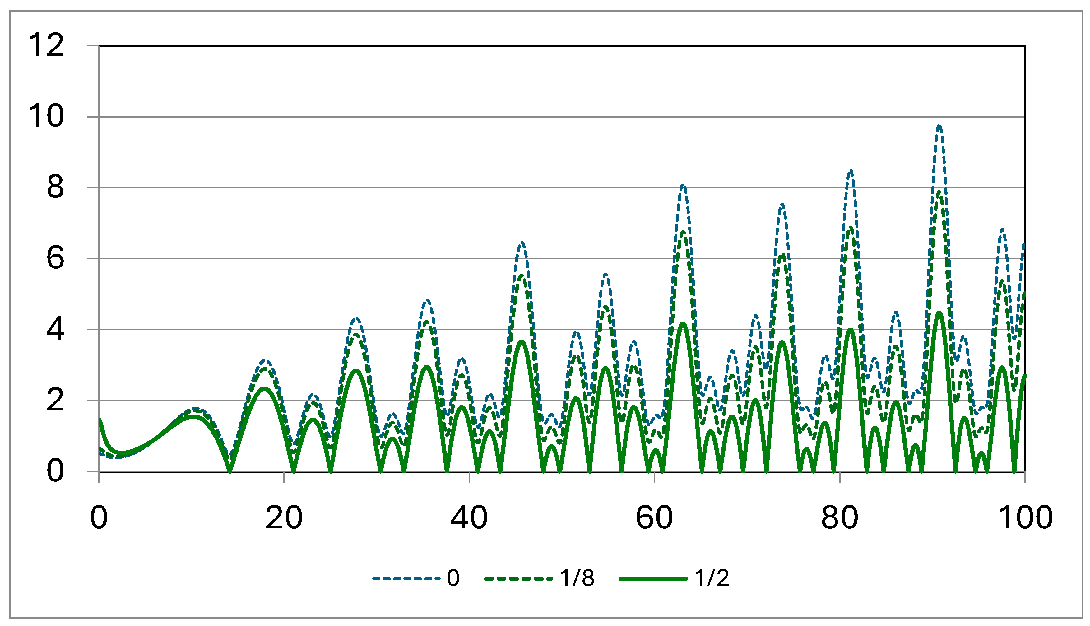
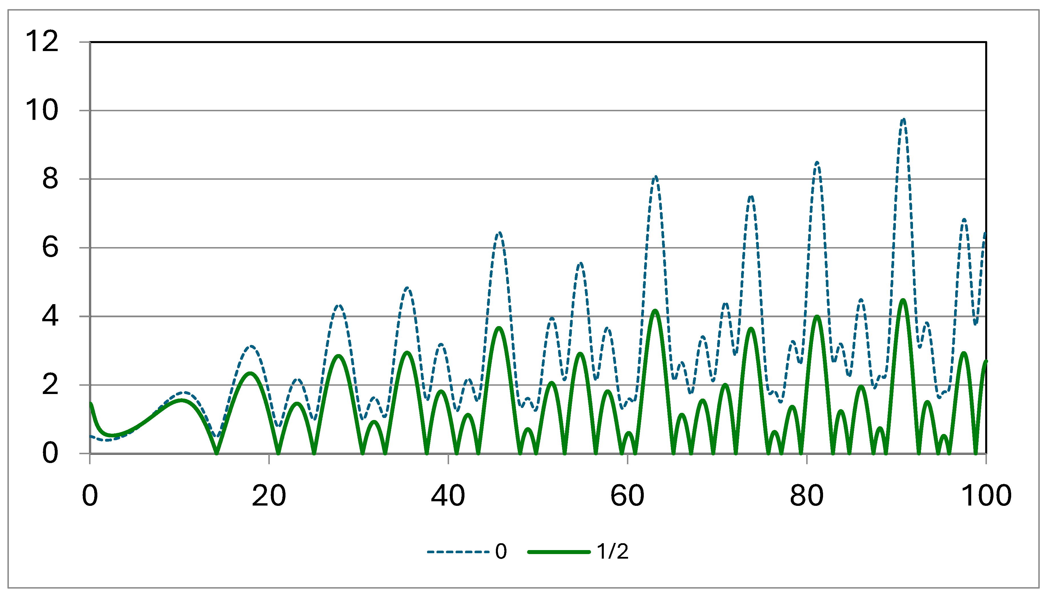
Figure 3.
Plots of | with
2.2.2. Determining the Value of “a” in
In the strip 0 < Re(s) < 1 this extension of
the zeta function satisfies the functional equation.
By using the following trigonometric relation and multiplying both equations 37 and 38 by cos (θ) and sin (θ), then add them.
First, convert equation 22 from cosine to sine, and
then add equation 23 to obtain equation 40.
By expanding equation 40 using the trigonometric
relation, we obtain equation 41.
Divide both sides of equation 41 by
In the second sentence of relation 42, we make a
small change because 1 minus 1 equals 0.
With the use of 44, we will have more options.
Once we have defined the relationships, we can
revisit the function, which is similar to relation #39.
If the expression equals to zero and the expression equals to one, then Relation 45 becomes similar to
Relation 39.
…+
To obtain a, the manipulation of function clauses
was only done in the second clause, which includes the prefix. The expression -1+1 is added to it, resulting in
a favorable outcome that confirms the correctness of Riemann's Hypothesis.
However, manipulating the remaining sentences yields new values for a, which
necessitates checking if there is a root on these new lines. We start from
Relation 42.
If the expression equals to zero and the expression equals to one, then Equation 48 becomes similar to
Relation 42.
If =0 , then: = = , a.= . , a= +
#
If the expression equals to zero and the expression equals to one, then Equation 50 becomes similar to
Relation 42.
If =0 , then: = , = ,a.= .
Analytical Proof:
According to Table 2, the root of ζ(1-s) lies between 1/2 and 1 if 0 < Re(s) ≤ 1/2, which is not possible. Therefore, values of a ≠ 1/2 cannot be the real part of the root of the zeta function. Thus, the function only has roots on the line Re(s) = 1/2. On the other hand, comparing of Tables 1 and 2, shows that the only common root between ζ(s) and ζ(1-s) is a=1/2.

Table 1.
potential values of the real part “s”, 0 < a ≤ , for
| n | 2 | 3 | 4 | 5 | 6 | 7 | 8 | … | m |
| a | 0.315464 | 0.215338 | 0.193426 | 0.178103 | … |
Table 2.
potential values of the real part “s”, ≤ a < for
| n | 2 | 3 | 4 | … | 8 | … | m |
| a | 0.684534 | … | … | 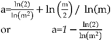 |
2.2.3. The Final Proof of the Riemann Hypothesis
The complex form of equations (5 and 18) for and are written.
By comparing both sides of equations 52 and 53, we can determine the value of "a".
Additionally, both the positive and negative values
of b can be used in equations 9 and 10.
Therefore, both and -b are valid for the function. The general
solution to the equation will be.
If we repeat this entire process with relation 1, we will obtain the same result with slight changes in the details (Shown in Appendix A).
2.3.4. Determining the Value of “b”
We start from Equation 2 to prove that the relation between the zeta function and prime numbers (Euler's relation) is true for >0.
. So we will have:
To determine the root of the equation, we set the
value of equal to zero and simplify the equation.
When solving the equation, terms with a factor of are placed on the left, while the remaining terms with a factor of one are placed on the right. Expressions that involve the multiplication of multiple primes in the denominator of the fraction are ignored with high confidence, compared to expressions that have only one prime in the denominator. The complete proof of the relationship between prime numbers and the generalized zeta function is given in Appendix B.
Therefore, the final form of the equation will be as follows.
2.2.5. Results
The correctness of Riemann's hypothesis has been proven by accurately determining that a=1/2. The real part of every nontrivial zero of the Riemann zeta function is Re(s) =Thus, the hypothesis is correct, and all the
nontrivial zeros lie on the critical line consisting of the complex numbers aib, where a=is a real number and b is the imaginary number.
In general, the following relationships hold for
the zeta function.
3. The Generator Function of Prime Numbers
First, we set the value of the original zeta function to 1. Using the trigonometric relationship, we convert it into a complex form and consider the real part as 1 and the imaginary part as 0. By summing the two real and imaginary components, we reach a value of a = 1/2.To find b’, we utilize the multiplicative form of prime numbers and set the value to 1 resulting in a new sinusoidal form of the real and imaginary parts which includes two parameters b’ and P. In this case, the amplitude of the zeta function is 1. With the correct assumption, the true value can be considered equal to the cosine of the arbitrary angle theta, and its imaginary part equal to the sine of the same angle. By using the relationship between the sine and cosine of the theta angle and solving the resulting equation, we obtained a correct relationship between b’ and the prime number corresponding to it.
The Riemann zeta function can be expressed in the following form for complex s.ζ ( s ) = ∑ n = 1 ∞ 1 n s = 1 1 s + 1 2 s + 1 3 s + ⋯
By utilizing the trigonometric relationship
provided, we are able to convert the shape of Riemann’s zeta function from
complex to sinusoidal form.
3.1. Determining the Value of a’
We multiply both equations 61a and 61b by and respectively, and then add them together.
We add the two relations 61a and 61b together to
obtain relation 63.
By expanding equation 64 using the trigonometric
relation, we obtain equation 61.
In the second sentence of relation 65, we make a
small change because -1+1 equals 0.
With the use of 66, we will have it.
Once we have defined the relationships, we can
revisit the function, which is similar to relation #59.
If the expression- is equal to zero and the expression () is equal to one, then Relation 67 becomes similar
to Relation 63.
Additionally, both the positive and negative values
of b can be applied in equations 61.
Therefore, both and -b’ are valid for the function. The general
solution to the equation will be
By substituting a =1/2, relations 60 and 61 are transformed into the following relations. Then by numerically solving the equation, we can determine the values of b’.
Similar to the proof presented in Section 2.2.4, the relation of prime numbers with the generalized zeta function is given in Appendix C.
When solving the equation, terms with a factor of are placed on the left, while the remaining terms
with a factor of one are placed on the right. Expressions that involve the
multiplication of multiple primes in the denominator of the fraction are
ignored with high confidence, compared to expressions that have only one prime
in the denominator.
Therefore, the final form of the equation will be
as follows.
3.2. Definition of the Generating Function of Prime Numbers
The real and imaginary components of equation 69
can be thought of as the cosine and sine of a trigonometric angle.
We can use the trigonometric relationship of the sum of the squares of sine and cosine to then obtain an independent relationship between b’ and the prime number.
3.4. Results
To find the values of b’, you can numerically solve
equation 67 and then calculate the corresponding prime number using equation
76.
In general, the following relationships hold for
the zeta function.
4. Conclusions
In this article, we began by attempting to prove
the Riemann hypothesis. We started by working with the initial form of the
function and then transformed it into its complex form. To find the roots of
the function’s real and imaginary values, we set it equal to zero. By
considering s = aib, we were able to derive the phase-shifted form
of the equation using trigonometric relations. Next, we combined the real and
imaginary parts of the equations (relations 9 and 10), expanded the resulting
equation, and compared it with the phase-shifted state. This process led to
obtaining two simple equations for values of a. Solving these equations
revealed that the value is equal to 1/2. Additionally, we applied the values
of b and -b in equations 9 and 10, confirming that all roots of the equation lie
on the line, resulting in s = aib.
It seems that obtaining a prime number generator
through the zero root of Riemann's zeta function is not possible. To create a
prime number generator function in terms of b’, one can solve the root of the
zeta function where it equals one (i.e., and establish a relationship between b’ and prime
numbers. By setting the value of zeta equal to one and s' = a' + ib’, similar
to zeta equal to zero, the roots are once again placed on the 1/2 line. Moving
forward, we will perform operations on equation 69, which represents the
complex form of the ∏ function. We assume that the real component is the cosine function and the imaginary component is the sine function. By using the trigonometric relationship that the square of the sine plus the square of the cosine equals one, we can derive an independent relationship between b’ and P. Therefore, if the value of b’ can be obtained from equation 61 as a numerical solution, then by using the relationship between b’ and P, referred to as the generating function of the prime number (relation 76), the prime number corresponding to b’ can be easily obtained.
Data Availability Statements
The data that support the findings of this study are openly available in [repository name] at https://www.claymath.org /[ sites/default/files/ezeta.pdf], reference number [1].
Declaration
On behalf of all authors, the corresponding author states that there is no conflict of interest.
Conflict of interest statement
We have no conflicts of interest to disclose.
Appendix A
The Riemann zeta function can be expressed in the following form for complex s:ζ ( s ) = ∑ n = 1 ∞ 1 n s = 1 1 s + 1 2 s + 1 3 s + ⋯
By using the following trigonometric relationship, we can transform the shape of Riemann’s zeta function from complex to sinusoidal form. eiθ
= cos(θ) + i sin(θ)
Before we begin proving the hypothesis, we first
obtain the Phase-shifted Riemann relation using the following trigonometric
relation, which we will reference at the end of the discussion.
Multiply both equations 7 and 8 by and , then add them together:
We combine relations 7 and 8 to obtain relation 16
By expanding the relation 16 using the following
trigonometric relation, we get:
Divide both sides of equation 17 by
In the second sentence of relation 18, we make a
small change because -1+1 equals 0.
With the use of 20, we will have.
Once we have defined the relationships, we can revisit the Phase-Shifted Riemann Zeta Function, which is similar to relation #14.
If the expression- is equal to zero and the expression () is equal to one, then equation becomes the Phase-Shifted Riemann Zeta Function (Relation 14).
Appendix B
To determine the root of the equation, we set the value of equal to zero and simplify the equation.
To simplify the multiplication process, the expression is changed from complex to exponential form.
With high confidence, expressions involving the multiplication of several prime numbers in the denominator of the fraction can be ignored compared to expressions containing only one prime number in the denominator.
Therefore, the final form of the equation will be as follows.
Appendix C
It can be concluded that
To simplify the multiplication process, the expression is converted from complex to exponential form.
When rearranging the terms of the equation, the terms with a factor of are placed on the left side, while the remaining terms with a factor one are included on the right side.
With high confidence, expressions involving the multiplication of several prime numbers in the denominator of the fraction can be ignored when compared to expressions containing only one prime number in the denominator.
Therefore, the final form of the equation will be as follows.
References
- Riemann, B. On the Number of Primes Less Than a Given Quantity. Available online: https://www.claymath.org/sites/default/files/ezeta.pdf (accessed on 30 December 2018).
- Hilbert, David (1900). "Mathematische Probleme". Göttinger Nachrichten: 253–297. Hilbert, David (1901). Archiv der Mathematik und Physik. 3. 1: 44–63, 213–237.
Disclaimer/Publisher’s Note: The statements, opinions and data contained in all publications are solely those of the individual author(s) and contributor(s) and not of MDPI and/or the editor(s). MDPI and/or the editor(s) disclaim responsibility for any injury to people or property resulting from any ideas, methods, instructions or products referred to in the content. |
© 2024 by the authors. Licensee MDPI, Basel, Switzerland. This article is an open access article distributed under the terms and conditions of the Creative Commons Attribution (CC BY) license (http://creativecommons.org/licenses/by/4.0/).
Copyright: This open access article is published under a Creative Commons CC BY 4.0 license, which permit the free download, distribution, and reuse, provided that the author and preprint are cited in any reuse.


