
Submitted:
19 August 2024
Posted:
20 August 2024
You are already at the latest version
Abstract
In this study, we propose a scalable deep learning approach to automated phenotyping using UAV multispectral imagery, exemplified by yellow rust detection in winter wheat. We adopt a high granularity scoring method (1 to 9 scale) to align with international standards and plant breeders’ needs. Using a lower spatial resolution (60m flight height at 2.5cm GSD), we reduce the data volume by a factor of 3.4, making large-scale phenotyping faster and more cost-effective while obtaining results comparable to those of the state-of-the-art. Our model incorporates explainability components to optimise spectral bands and flight schedules, achieving top-3 accuracies of 0.87 for validation and 0.67 and 0.70 on two separate test sets. We demonstrate that a minimal set of bands (EVI, Red, and GNDVI) can achieve results comparable to more complex setups, highlighting the potential for cost-effective solutions. Additionally, we show that high performance can be maintained with fewer time steps, reducing operational complexity. Our interpretable model components improve performance through regularisation and provide actionable insights for agronomists and plant breeders. This scalable and explainable approach offers an efficient solution for yellow rust phenotyping and can be adapted for other phenotypes and species, with future work focusing on optimising the balance between spatial, spectral, and temporal resolutions.
Keywords:
deep learning
; yellow rust
; wheat breeding
; XAI
; multispectral data
; UAV
; remote phenotyping
; vegetation indices
1. Introduction
Amid growing concerns over food security and the stagnation of global crop production [1], there is a pressing need to enhance the scalability of agricultural innovations, particularly in the realm of plant phenotyping. As wheat is a staple crop consumed globally, improving the resilience and yield of winter wheat (Triticum aestivum L.) through advanced breeding techniques is vital for ensuring food security [2]. To this end, remote phenotyping, which utilises non-destructive sensors and cameras to measure plant characteristics, has emerged as a pivotal technology. It offers a more scalable alternative to traditional, labour-intensive methods of genotype selection [3].
Focusing on the scalability of automatic phenotyping systems, this paper studies the case of yellow rust, or stripe rust-affected (Puccinia striiformis) [4] winter wheat, to explore the effectiveness of these technologies in a multi-temporal set-up. Numerous countries worldwide have experienced large-scale yellow rust epidemics in the past [5,6,7]. In 1950 and 1964, devastating yellow rust epidemics in China resulted in estimated yield losses of 6.0 and 3.2 million tons, respectively [6]. [7] reported a severe yellow rust epidemic in Central and West Asia with yield losses ranging from 20% to 70% across countries. In the 1960s and 1970s, around 10% of Europe’s yield was lost due to yellow rust [8]. The most recent significant outbreak identified occurred in the United States in 2016 with average losses of 5.61% across the country, resulting in a total loss of approximately 3.5 million tons [9]. Multiple approaches can mitigate yield losses caused by yellow rust, including the development and use of resistant cultivars [10]. Since new yellow rust races continuously emerge, posing a threat to existing resistant cultivars [10], this approach requires their continued renewal. This underscores the need for ongoing yellow rust resistance testing and the development of new resistant cultivars, and justifies the need of efficient phenotyping strategies for the foreseeable future.
In the realm of agricultural research, the integration of cutting-edge technologies has become pivotal in combating crop diseases such as yellow rust. One promising avenue involves harnessing Machine Learning (ML) to analyse multispectral imaging data sourced from UAV flights or other platforms [11]. UAVs are particularly helpful since they can cover large amounts of agriculture fields and carry different types of multispectral and hyperspectral sensors [12,13]. This synergy between remote sensing and ML promises powerful solutions for detecting yellow rust susceptibility or resistance [14]. Several groups proposed approaches for yellow rust monitoring. Table 1 presents an overview of the most important ones.
We differentiate ourselves from these studies in 3 key scalability aspects:
- most of these studies gather the measurements used for phenotyping using phenocarts or handheld devices. We use UAV imagery, a more scalable solution which can be easily applied to new fields;
- all of these studies consider high to very high resolution data, with non-UAV studies acquiring data at very close range and UAV flights going up to 30m of altitude. We want to favour lower volumes of data and faster acquisition with regular and standardised flights from an altitude of 60m at high accuracy using fixed ground control points (GCP);
- none of these studies adhere to agricultural standards of disease scoring, instead only distinguishing between 2 or 3 classes most of the time.
In the following paragraphs, we study those current trends and their drawbacks in more detail.
In terms of time and hardware needed, [15,16,17,18] use phenocart and images acquired by handheld devices to make the predictions. Although this presents an inherently easier machine learning problem [15], we prefer the UAV solution which simply requires flying a drone over the field. This is non-intrusive [22] (ie., it does not require to adapt the field to the phenotyping method), and requires little time from the perspective of the human operator. To leverage this in [19,20,21], UAVs are employed for yellow rust monitoring. Nevertheless, those approaches have several drawbacks.
Flying a drone can be a time-comsuming endeavour if the target resolution is high. High spatial resolution images are very rich, and can be exploited by deep learning convolutional modules to extract image patterns, textures and more generally spatial components [23]. When using high spatial resolutions, the yellow rust pustules are visible and a deep vision model can identify them [15]. However, this leads to larger data volumes, which implies higher hardware requirements. It also significantly increases the flight time, which in turn may lead to the necessity to change the drone’s batteries more often. [19] uses a drone hovering at 1.2 m above the canopies, leading to extremely high data throughputs. [21] operates at a more efficient 20m of altitude, but this remains insufficient to efficiently capture large areas. Finally, [20] uses a hyperspectral camera and fly at 30m of altitude, but although hyperspectral cameras provide very rich data, they are particularly expensive. In our research, we adopt a much higher flight altitude of 60m and include more spectral bands (RGB, Red Edge, NIR) to assess how spectral resolution [24] can counteract this lack of spatial resolution. We also try to develop a model that, through the usage of fewer spectral bands and indices; as well as less frequent UAV acquisition, can yield good performance and scale further remote phenotyping. However, in contrast to [20], we do so conservatively and attempt to study which bands contribute the most for future optimisation.
The results present in the literature, reported in Table 1, appear solid, with accuracies as high as 99% on the binary healthy/unhealthy regression problem [15] and 97.99% on the 6 class problem [18]. However, it is important to note that while many approaches focus on the binary healthy/unhealthy problem in yellow rust prediction, this scale is often insufficient for breeding operations. In our study, we scored yellow rust following the official Austrian national variety testing agency AGES (Austrian Agency for Health and Food Safety GmbH) on a scale from 1 to 9. The Federal Plant Variety Office in Germany also uses a comparable scoring system from 1 to 9 for yellow rust disease occurrence. Various other methodologies exist for measuring or scoring yellow rust damage, including evaluating per cent rust severity using the modified Cobb Scale [25], scoring host reaction type [26], and flag leaf infection scoring [27]. For instance, [28] utilised continuous disease scoring from 1 to 12 throughout the season to evaluate the area under the disease progression curve. These scoring scales are designed for the context of plant breeding to be useful in a variety of situations, comparable to international standards and results, and also from one dataset to another. In contrast, the number of target classes used in the literature is extremely coarse, which makes it hard to validate, generalise and share across different domains.
Our proposed approach, TriNet, consists of a sophisticated architecture designed to tackle the challenges of yellow rust prediction. TriNet comprises three components - a spatial, a temporal, and a spectral processor - which disentangle the three dimensions of our data and allow us to design built-in interpretability in each of them. TriNet maintains performance levels comparable to the state-of-the-art, despite the difficulties introduced by higher operational flight heights and thus lower spatial resolutions. Furthermore, TriNet generates interpretable insights through the importance of attention weights. This facilitate more informed breeding decisions. We leverage domain knowledge during model training thanks to the interpretability offered by attention weights present in the spatial, temporal, and spectral processors, which we hope to be a promising avenue for fostering the development of more robust and generalisable models.
In this study, we claim the following contributions.
- We achieve promising results in terms of top-2 accuracy for yellow rust detection using UAV-captured images taken from a height of 60 metres (see Table 5).
- We introduce a modular deep learning model, with its performance validated through an ablation study. The ablation is applied to the architectural elements as well as the spectral components and the time steps (see Section 3.3 and Section 3.5).
- We demonstrate the interpretability of our model by showing that it can offer valuable insights for the breeding community, in particular showcasing its ability to select important bands and time steps (see Section 3.4). We believe these results to be an important step forward for scalability in remote phenotyping.
2. Materials and Methods
2.1. Study area and experiments
We study the growth and development of yellow rust in winter wheat in Obersiebenbrunn, Austria. The agricultural research facility in Obersiebenbrunn is overseen by the plant breeding organisation Saatzucht Edelhof [29].
The experiments is performed in the season 2022/23 on chernozem soil. The mean annual temperature is 10.4°C and the mean annual precipitation is 550 mm. Plots of winter wheat genotypes at various stages in the breeding processes were established with 380 germinable seeds m-2. Exceptions are the experiments WW6 and WW606, which consist of four commercial cultivars (Activus, Ekonom, Ernestus and WPB Calgary) in four different sowing densities (180, 280, 380 and 480 germinable seeds per square metre) in one replication for both WW6 and WW606 respectively. The pre-crop of the field is sunflower. The seedbed was prepared using a tine cultivator to a depth of 20 cm. Sowing was performed on October 18th 2022 with a plot drill seeder at a depth of 4 cm. Fertilisation as well as control of weeds and insects was conducted in accordance with good agricultural practice. No fungicides were applied.
The field is organised into 1064 experimental plots where the experiments are conducted. To identify each plot, we use the notation system Y-G-R structured as follows:
- Y represents the year in which the genotype reached the stage of experimental yield trials in the breeding process. The experiments, however, also include check cultivars, which are genotypes that are already on the market and used to compare the performance of genotypes in development to the current cultivars on the market. These commercial cultivars are denoted as "COMM.".
- G denotes the name of the genotype planted in the plot.
- R signifies whether the plot serves as a replication for statistical robustness. It is followed by a numerical value (R1 or R2) to distinguish between different replication instances.
For instance, a plot identified as Y[21]-G[SE 001-21 WW]-R[2] indicates the seed genotype SE 001-21 WW was selected in the year 2021 (Y21), and out of our two replicated plots with these characteristics, this is the second one (R2). 168 plots of the fields are sown with commercially available genotypes. 36 of these are treated as a control group and we assign them the identifier "COMM.". This metadata is used to determine relevant data splits for machine learning in Section 2.3. To visualise the distribution of these traits please consult Figure 4.
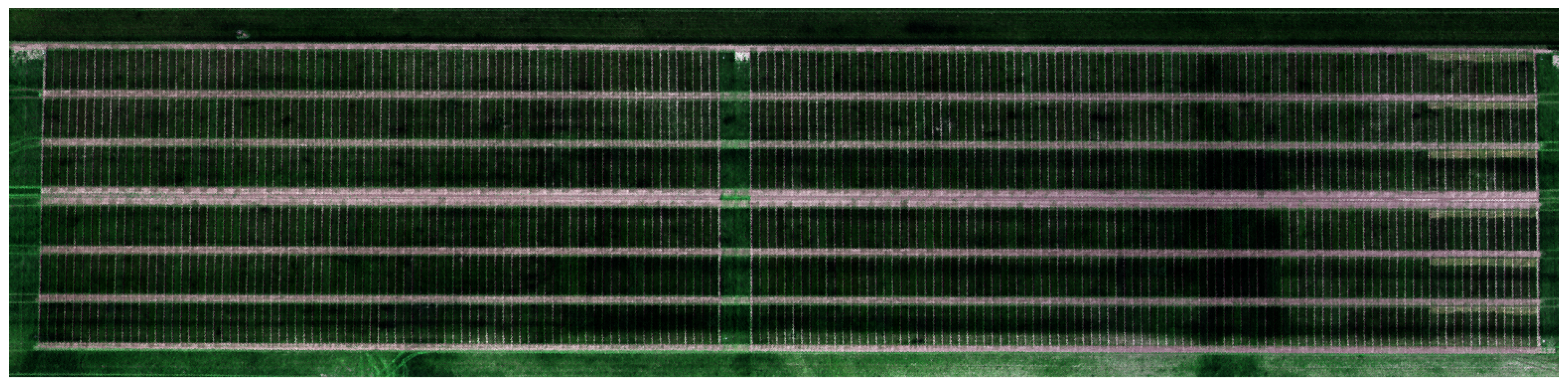
Figure 1.
RGB aerial view of the field in Obersiebenbrunn on 27th April 2023.
As previously stated, yellow rust was scored in this study according to the official Austrian national variety testing agency AGES (Austrian Agency for Health and Food Safety GmbH). Therefore, yellow rust severity was scored on a scale from 1 to 9. The individual scale levels from 1 to 9 are defined as follows: 1 no stripe rust occurrence, 2 very low or low occurrence (only individual pustules), 3 low occurrence (many plants with few symptoms or few plants with medium symptoms), 4 low to medium occurrence, 5 medium occurrence (many plants with medium symptoms or few plants with many symptoms), 6 medium to high occurrence, 7 high occurrence (all plants with medium symptoms or many plants with many symptoms), 8 high to very high occurrence, 9 very high occurrence (almost all leaf and stem areas are covered in pustules).
2.2. Sensor and data acquisition
For this study, we acquired a time series of multispectral data with a UAV. This drone platform is well-suited for its capacity to carry substantial payloads, including a multispectral camera. The camera utilised in our study is the Altum-PT model [30], weighing 0.5 kg, capable of capturing RGB, Red Edge, NIR, LWIR, and panchromatic bands. For the sensor specifics see Table 2.
The UAV maintains a flight altitude of 60 metres, resulting in a Ground Sampling Distance (GSD) of 2.5 cm for the multispectral bands, 16.7 cm for the LWIR band and 1.2 cm for the panchromatic band. This GSD is larger than most existing UAV-based yellow rust monitoring approaches. For instance, in [20], the flight altitude is 30 m (~2 cm GSD), in [19], it is 1.2 m (0.5 mm GSD), and in [21], the height is 20 m (1 cm GSD). In our study, we contribute to investigating the tradeoff between model performance and GSD by choosing a higher flight altitude. Specifically, we choose a GSD of 2.5 cm. While being much higher than competing studies to assess the possibility of performing phenotyping from this height, this GSD closely matches the size of wheat flag leaves, which are pivotal for evaluating wheat plants [31]. Therefore, this seems to be a good starting point to evaluate the potential of higher-altitude flights in wheat phenotyping.
To thoroughly understand the potential of this lower GSD for remote phenotyping, we perform a rich multispectral and multi-temporal acquisition paired with expert-assessed yellow rust disease scores. Throughout the winter wheat growth period, we conduct a total of 7 flight missions from March to June to gather data in our test fields. The specific dates are reported in Appendix 10.
During each flight, our drone captures approximately 320 multispectral images following a predefined path covering 282 x 57 metres of the entire experimental field with an overlap of at least 6 images per pixel. These images are subsequently orthorectified, radiometrically calibrated, and stitched together, as comprehensively detailed in [32]. All flight campaigns were conducted around noon to ensure consistent lighting conditions. We performed radiometric calibration using a two-step approach: pre-flight calibration with a reflectance panel for each band and in-flight correction using a Downwelling Light Sensor (DLS) to account for varying ambient light. The data was processed using Pix4Dmapper, which also addressed potential spectral mixing issues. The combination of standardised calibration, consistent flight patterns, and high image overlap helped to minimise radiometric and geometric distortions in the final dataset.
One important feature of our data acquisition is using ground control points (GCPs), as in [33], to enhance the geolocalisation of the UAV’s images. The outcome of this process is a tensor comprising 7 spectral channels and covering the entire field. However, this reflectance map is not readily usable as a machine-learning dataset. As a reference, the acquired data in our set-up with an operational height of 60 m is 1.74 GB, while it is 5.96 GB when flying at 20 m. This large difference in data volume significantly speeds up the preprocessing to obtain the reflectance maps using pix4D (by a time factor of 4).
Four external points of known geolocation delineate the boundaries of each plot. As described in [32], these points serve as reference coordinates to resample the plot quadrilateral into a rectangular matrix of reflectance values using a homography transformation to eliminate the effect of geographic raster grid alignment. In Figure 2 we present a diagram illustrating the transition from the larger reflectance map to the resampled plot.
In our case, we use bicubic resampling to reconstruct the pixel values in our final plot data. In this procedure, we maintain high absolute geolocation accuracy through the use of GCPs. Having square images with no borders around the fields makes them easier to use in the context of deep learning, in particular, so that flip augmentations follow the axes of symmetry of the fields and only the relevant portion of the image is kept. This is particularly significant as we are, among other things, interested in measuring the intensity of border effects on the chosen phenotype. This procedure is applied to each of the drone flights. The result is a tensor with the following dimensions:
- Plot Number (length 1025): denoted p, a unique identifier assigned to each experimental plot within the research facility.
- Time dimension (length 7): denoted t, the date when the multispectral images were captured.
- Spectral dimension (length 7): denoted , the spectral bands recorded by our camera, plus the panchromatic band.
-
Spatial dimensions collectively denoted :
- −
- Height dimension (length 64): denoted h, the height of one plot in pixels.
- −
- Width dimension (length 372): denoted w, the length of one plot in pixels.
2.3. Dataset Preparation
We add several spectral indices tailored to describe specific plant physiological parameters [34]. These indices have been shown to effectively describe wheat plants’ health and growth status [35]. In general, spectral indices elicit more information from the data than raw spectral bands, and have long been used in plant science as high-quality features. We selected a total of 13 indices that we report in Table 3.
These 13 indices, which constitute information regarding the physiology of the plant, are computed and then added as new channels to the dataset tensor, resulting in 20 channels. Introducing domain-motivated features in the form of those spectral indices acts as an inductive bias to converge to better results despite our comparatively low data regime. In other words, they constitute already valuable information that the model does not need to learn to derive from the input data, and guides the model towards a solution that makes use of these specific characteristics of the input bands.
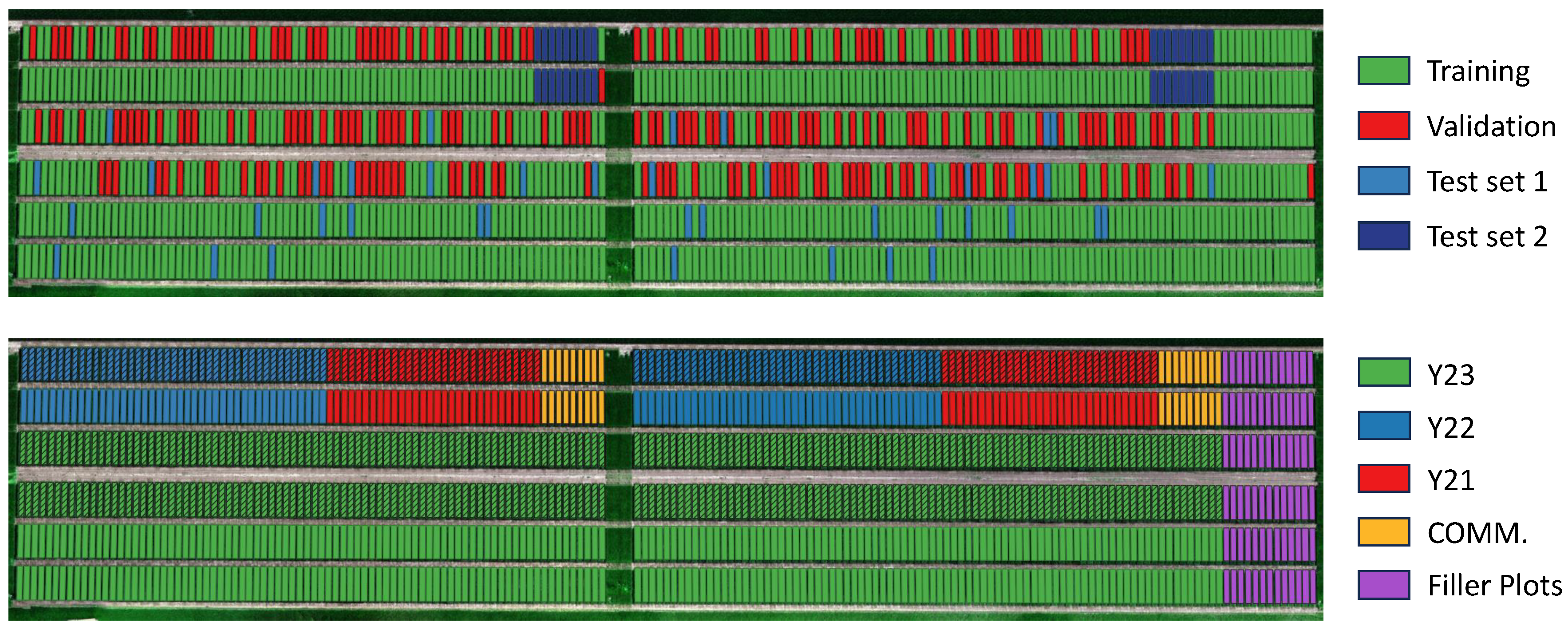
We then divide the dataset into four distinct sets: train, validation, and two test sets to evaluate different characteristics of our models. This split is based upon the operational division employed by agronomers, as visible in Figure 4. In Table 4 we present a summary.
- Test set 1: this set comprises 10 genotypes selected from the breeds initially selected in 2023, 2022 and 2021. This test set aims to match the distribution of the training and validation sets. To ensure a comprehensive evaluation despite our unbalanced labels, we ensured similar class distributions across train, validation and test set 1. This set tests our model’s overall generalisation capabilities.
- Test set 2: this test set includes plots whose genotypes are commercially available. Its primary function is to act as a control group, assessing the algorithm’s ability to generalise to genotypes selected in previous years by different wheat breeding companies. However, it is worth noting that this dataset is unbalanced, with a predominance of low disease scores.
- Validation: this set is composed by 54% of the Replication 2 of the remaining plots, totalling 222 time-series. This set serves as a set to validate the training results, comparing model trained with different architectures and hyperparameters and fine-tuning the hyperparameters.
- Train: The remaining experiments compose the training set. This set has 726 time series of multispectral images.

Table 4.
Description of our data splits for machine learning. In test set 1 stands for genotypes not previously selected. There is no overlap between breeds/genotypes represented by and X. COMM. refers to commercially available genotypes.
Table 4.
Description of our data splits for machine learning. In test set 1 stands for genotypes not previously selected. There is no overlap between breeds/genotypes represented by and X. COMM. refers to commercially available genotypes.
| Split | Cardinality | Identifiers |
|---|---|---|
| Train | 726 | Y[20/21/22]-G[X]-R[1], Y[20/21/22]-G[X]-R[2] |
| Validation | 222 | Y[20/21/22]-G[X]-R[2] |
| Test 1 | 41 | Y[20/21/22]-G[]-R[1], Y[20/21/22]-G[]-R[2] |
| Test 2 | 36 | COMM. |
This split provides a robust setup for various machine-learning experiments. Figure 3 provides a visualisation of the distribution of the targets in the four sets.
Figure 3.
Distribution of the target classes in the four sets. The data are acquired the 24th of May 2023.
Figure 3.
Distribution of the target classes in the four sets. The data are acquired the 24th of May 2023.
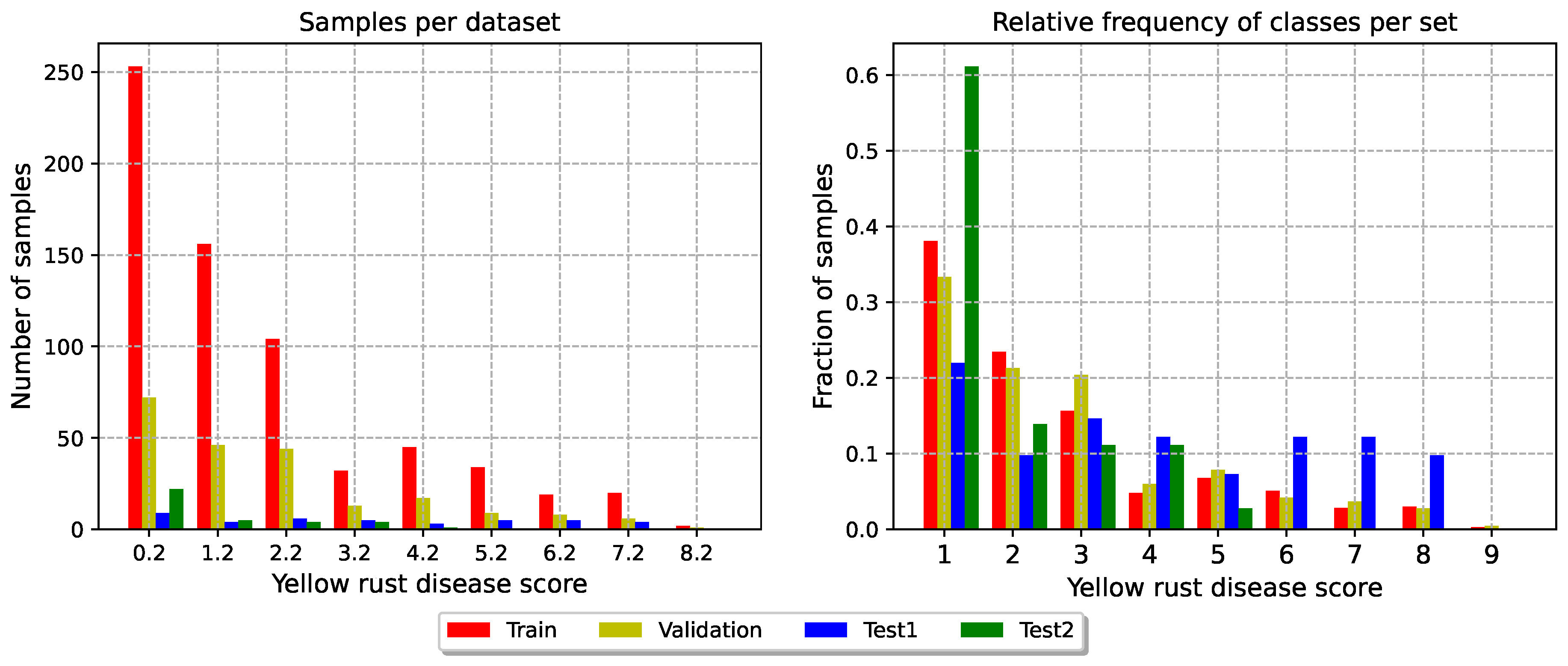
Figure 4.
Spatial distribution of the plots. In the upper image the data split is presented. In the bottom image the year the genotypes are selected is presented. The striped plots (i.e., row 3 and 4) are referred to replication 2 (R2) while the others are referred to replication 1 (R1). The filler plots are automatically removed from the data pipeline, since they do not have an associated phenotype score.
2.4. TriNet Architecture
In this study, we propose TriNet, a deep learning model designed to solve the task of remote phenotyping of yellow rust while providing insights to make acquisition operations more resource efficient in the future. For example, we hope to learn which bands are the most impactful for the performance, or at which time steps it is the most important to acquire data. TriNet consists of three distinct stages which each independently process one of the problem’s dimensions: the spectral processor, the spatial processor, and the time processor. A schematic representation illustrating the various parts can be found in Figure 5.
- Spectral processing stage: the model identifies the most pertinent spectral bands and vegetation indices dynamically during training.
- Spatial processing stage: the model’s feature extractor extracts patterns from the image data. Then, it collapses the two spatial dimensions width and height by averaging the features, facilitating the processing of the time dimension.
- Time processing stage: the model captures and exploits temporal dependencies within the time series data, trying to make use of different kinds of information from different growth stages.
2.4.1. Attention Layers in TriNet
Each of these stages harnesses the concept of attention, originally introduced in [51] in the context of machine learning. Different kinds of attention have been used across the literature until self- and cross-attention, where attention weights are derived from the input data itself, became the main components of some of the most powerful known models in natural language processing [52] and computer vision [53]. Attention was originally added to neural networks as a pivotal building block to adaptively and dynamically process spatial features and patterns, as well as an interpretable component that made it possible to draw insights into the model’s inner workings. In our implementation, we focus on the interpretability of attention layers, and therefore use the simpler original attention from [51] with one or several attention heads.
Single-head attention essentially computes a weighted average of input features along a given dimension, with the weights indicating the relative importance of each feature. By extension, multi-head attention generates multiple feature-weighted averages by applying independent sets of weights. Our aim is to select generally better spectral bands or time steps for yellow rust remote phenotyping, as well as to understand the impact of the relative location inside the plot when monitoring yellow rust. Therefore, constant learnt attention weights are the tool of choice for our purpose, as opposed to self-attention for example.
Mathematically, we can write an attention function with h heads operating on dimension k as a parametric function , where is a tensor with D dimensions, and can be seen as h vectors of one weight per element in X along its dimension. With a single head, will collapse X’s dimension, giving as output a tensor . If we denote the tensor slice corresponding to the element of X along the dimension, single-head attention can be written as:
where w, in the 1-head case, is simply a vector of elements, and softmax is the softmax function [54] (such that the weights used for averaging are positive and sum to 1). From this, the general h-heads case gives as output a tensor , where the element along the dimension is the output of the head and can be written as:
In what follows, we typically refer to dimensions by name instead of by index, for example is a h-heads attention along the spectral dimension of a plot denoted X.
2.4.2. Spectral Processor
Let our input plot be a tensor with dimensions [t, sc, h, w]. Our spectral processor (see Figure 5) selects the bands and spectral indices to use in the subsequent processors. We seek to both better understand the contributions of our bands and indices and minimise the complexity of the following spatial processor (see Section 2.4.3). Therefore, in this processor, we have a strong incentive to aggressively select as few bands as possible so long as it does not degrade the model’s performance. Re-using the formalism established in Section 2.4.1, this processor can simply be written as one h-heads attention layer, with h the number of spectral bands and indices we want to keep in the output :
The output still has dimensions [t, sc, h, w], but now the dimension contains h composite bands each created from performing attention on the input bands and indices.
2.4.3. Spatial Processor
The spatial processor consists of three parts as shown in Figure 6: spatial processing, then chunking the plot along its width into several areas, then spatial attention between those areas.
In this module’s first section, we extract spatial features which we then use as predictors for the presence of yellow rust in subsequent steps. We design our spatial feature extractor based on several key hypotheses:
- Our UAV observations have a relatively low resolution where individual plants are not always discernible. Therefore, we hypothesise that the features should focus on local texture and intensities rather than shapes and higher-level representations;
- although yellow rust’s outburst and propagation may depend on long-range factors and interactions within the plots, measuring the presence of yellow rust, is a local operation which only requires a limited receptive field;
- because we care more about local information on textural cues (i.e., high-frequency components), essentially computing statistics on local patterns, a generically-trained feature extractor might suffice. In addition, because of this generality, the same feature extractor might work for all input band composites in the spectral processor’s output.
To make use of these hypotheses, we choose a pre-trained deep feature extractor denoted , which we keep frozen. Early experiments with non-pre-trained feature extractors do not converge, which we interpret as our dataset is too small to train the significant number of parameters they contain. In this study, we use ResNet-34 [55] as our feature extractor. ResNet-34 proved to be efficient in predicting yellow rust in other studies using low altitude UAV images [20,56] or mobile platforms [57]. We experiment with various shallow subsets among the first layers of ResNet-34, to avoid higher-level representations in line with our hypotheses. Finally, since ResNet-34 is pre-trained on RGB images, it expects 3 channels. Therefore, we use a function denoted to recombine our input channels into groups of three to satisfy this requirement. More details are given in Appendix B. The extracted feature maps from each group of three input channels are then concatenated back together.
In the second part of the spatial processor, the plot’s feature maps are chunked along the width dimension. This allows us to apply attention to different locations in a plot. At a glance, this might not seem intuitive, because it would seem more natural to consider each plot chunk equally to evaluate the average health. Although it introduces additional parameters and sparsity to the model which might make it harder to train, allowing the model to focus unequally on different chunks allows us to verify this assumption:
- if some spatial chunks of the plot contain biases (e.g.,; border effects or score measurement biases), the model might learn unequal weights;
- if no such biases exist we expect the model to attend equally to all chunks.
The result of our chunking is a tensor of dimensions [t, sc, ck, w, h], where a new dimension stores the chunks and the new width along dimension w is the width of the features maps divided by the number of chunks. This chunking operation is denoted . We post-process the chunks with batch normalisation (denoted ) and a ReLU activation (denoted ), following standard techniques in image recognition [58]. The use of batch normalisation in the latent space of deep architectures has been shown to facilitate convergence across a wide variety of tasks. The third part of the spatial processor then applies attention to the chunks.
Now that a potential bias in the chunk location has been accounted for, we assume that the plot’s overall health is the average of the local health over all locations. Therefore, we collapse the spatial dimension of our data by averaging all features - our predictors for the plot’s health - across their spatial dimension. We call this operation .
At each time step, we obtain a vector of global features describing the plot’s spatial and spectral dimensions. Using the notations presented throughout this section, we get the expression of the output of the spatial processor concerning the output of the previous spectral processor:
The output has dimensions [t, f], with f the dimension of the new spatial features.
2.4.4. Feature Selection
Since we use a generically trained feature extractor, it is reasonable to assume that most of the extracted features do not correlate well with the presence of yellow rust. A natural step to take before processing the plot data along its time dimension is to further select from the features useful for the task at hand. We use a single fully-connected layer which we denote , because of its L1-regularised weights, as a selection layer with a slightly higher expressive power than an attention layer due to its fully connected nature. L1 regularisation guides the weights towards sparser solutions, meaning that the weights will tend to collapse to zero unless this decreases performance, hence selectively passing only useful information to the next layer. It is also followed by an additional rectified linear unit (). Here, and in general, we add such layers as non-linear components that also introduce sparsity by setting negative activations to zero and thus reducing the number of active features. The output has the same dimensions as but contains a smaller number of extracted features for each time step.
2.4.5. Time Processor
The last dimension of our data - time - is processed by our Time Processor. The spatial features at each time step are first processed together by layers of Long-Short Term Memory [59] cells with neurons, which we collectively denote . Long-Short Term Memory cells have been a long-used architectural component in deep architectures to process time series data differentiably [60]. The features in the output of this layer finally encode the information in the three spectral, spatial and temporal dimensions. The Long Short Term Memory layers are followed by another and a single head attention on the t dimension. Intuitively, we want the model to learn which are the flight dates that contribute the most to detecting yellow rust, hence the use of attention once again. The output is a simple vector containing rich features encoding all the dimensions of the input data and is obtained as shown in Equation 3. The importance of how much a single timestep contributes to the regression problem is represented by the magnitude of the weight , with t being associated to one of the dates reported in Table 10.
2.4.6. Regression Head
We compute our regression outputs with fully connected layers with neurons and layers as activations, followed by a fully connected layer with a single neuron and no activation. These layers are collectively denoted as , which yields the final output of our model.
2.4.7. Loss Function
We train TriNet with the Mean Squared Error, denoted between the predicted yellow rust score (between 1 and 9), and the score obtained during our expert scoring (see Section 2.1).
We also regularise some weights with different loss functions to encourage the model to exhibit specific behaviours. As explained in Section 2.4.4, we want the feature selector to aggressively select which features to keep for the subsequent steps. The rationale behind it is that ResNet generates a high number of channels in its output and not all of them contribute to the model’s output. By introducing this generalisation we nudge the model into the direction of excluding those channels. For this purpose, the weights of our layer are regularised by their norm as in standard Lasso[61].
In this study, one of our main goals is to analyse which bands, indices and time steps are the most influential in order to simplify future studies. Therefore, we also add entropy losses to all our attention weights. Intuitively, minimising entropy means favouring sparser attention weights, or in other words, more selective attention layers. For attention weights w, we consider the entropy :
We apply entropy to the weights of each head in Equation 1, the weights in Equation 2 and the weights in Equation 3.
To each additional loss we assign a scalar to serve as regularisation term, leading to the loss function:
with TriNet our model, the input data and y its associated ground truth score.
3. Results
We conduct extensive experiments to use our proposed TriNet architecture for our two main purposes:
- training a state-of-the-art model for yellow rust phenotyping at a 60 metres flight height (see Section 3.2);
- gaining insights into efficient operational choices for yellow rust remote phenotyping (see Section 3.4).
3.1. Metrics
We evaluate TriNet using a set of carefully chosen metrics. Our model outputs a single number which is a regression over the possible scores (between 1 and 9). Therefore, traditional regression metrics (in our case, and ) naturally make sense to compare our results. However, they do not constitute the best way to assess the practical usability of our model because we want to develop a tool usable and interpretable by breeders and agronomists. Since in the field several classification scales are used, we transform the regression problem into a classification one, by considering each integer as an ordered class. As a consequence, we also propose to use classification metrics, and further report the top-k accuracy metric. In our case, we assume the top k predicted classes to be the k closest classes to the predicted score. For example, if we predict , the top 3 classes are 3, 2 and 4 from the closest to the furthest. top-k accuracy therefore describes the percentage of samples in a set for which the correct class is among the k closest classes.
Classification metrics are useful to plant breeders, because they need to know approximately which class a certain field is classified as, and group several classes together to make decisions [62]. These groups of classes can vary based on the application and the breeders, hence why the entire scale from 1 to 9 is necessary in general. Therefore, we need metrics to inform on the capacity of the model to give accurate scores, but also metrics to inform on its capacity to give approximate scores at different resolutions. This is also useful for fairer comparisons to existing literature with fewer classes. The class groups used to obtain a certain binary or ternary score are unknown, and we therefore choose top-k accuracy metrics as a good compromise.
We generally report top-3 accuracy as our metric of choice from an interpretability perspective, which corresponds to being within 1 class of the correct class. We also report top-1 and top-2 accuracy for completeness. We hope to give the reader a better intuition of how to compare this model to 2-classes or 3-classes formulations usually present in yellow rust monitoring literature [15,16,17,19]. We chose this because comparing results between a 2-class and a 9-class problem presents significant challenges. Simplifying a 9-class problem by grouping classes into 2 broad categories is inherently imprecise. It raises the issue of how to appropriately group these classes and overlooks their natural ordering. For example, if classes 1 to 4 are grouped into a "negative" category, then a predicted class of 5 or 9 would be incorrectly classified as equally significant true positives, which is a poor representation of reality.
Top-k accuracy offers a more nuanced solution. This classification metric accounts for how close the model’s prediction is to the actual score, thereby providing insight into how a 9-class problem might be translated into various 2-class or 3-class versions without arbitrarily deciding on specific groupings. It also accounts for the class ordering in a finer way than binary or ternary classification does.
In a binary classification framework with a threshold (e.g., class 3; see [63]), the ordering plays a critical role. Binary classification checks whether the true value exceeds a certain threshold, effectively utilising the ordered nature of the classes. Thus, the inherent order in the regression problem facilitates a comparison of top-k accuracy, which measures the closeness of a prediction to the true value, with binary classification, which determines whether the true value surpasses a specified threshold. This approach provides a method to compare our regression study’s performance with other studies in the literature, bridging the gap between multi-class and binary classification analyses.
3.2. Base Model
First, we optimise TriNet to obtain the best phenotyping quality possible at our operating height. We extensively experiment with our validation set to find the following values:
- using as our number of heads in the spectral attention layer;
- the number of pretrained modules in our feature extractor1;
- using chunk in our spatial processor (meaning we do not chunk the data spatially);
- the number of output channels for our feature selector;
- the number of LSTM layers and their internal layers’ size ;
- the number of hidden layers and their number of neurons in the regression head;
- the loss components , and ;
- the learning rate , multiplied by every 30 epoch for 200 epochs, with a batch size of 16. We also apply a dropout of on the ’s hidden layers and the LSTM’s weights. We use a weight decay of and clip gradients of norm above 1. We report the model that achieves the highest validation score during training.
In addition, we notice that using statistics tracked during training at inference time in batch normalisation layers hurts the performance significantly, and therefore use online-calculated statistics contrary to popular convention. We interpret this as the model needing precise statistics to perform regression, contrary to a discrete task such as classification. This problem is also further exacerbated by the small size of the training dataset since the running means are not good descriptors for each possible subset of data.
Two parameters are of particular note here. First, using no chunks seems better than using chunks for spatial processing. This would imply that training additional per-chunk weights is an unnecessary overhead for the model and that all locations within a plot should be considered equally. We will come back on this conclusion in future sections. Second, our base model was achieved with un-regularised bands attention weights. As we will see, using bands selected that way is still conclusive, although a stronger regularisation would have lead to a clearer selection.
With these parameters, we obtain our best results for yellow rust phenotyping at 60 metres of altitude with scores from 1 to 9. We report our results in Table 5 with a 90% confidence interval obtained via bootstrapping with 100 000 resamplings of size equal to the original dataset size. All confidence intervals in this paper are reported this way.
Table 5.
The Mean Square Error (MSE), the Mean Absolute Deviation (MAD), and some top-k accuracy results on all sets for our base model.
Table 5.
The Mean Square Error (MSE), the Mean Absolute Deviation (MAD), and some top-k accuracy results on all sets for our base model.
| Data split | MSE | MAD | Top-1 Accuracy | Top-2 Accuracy | Top-3 Accuracy |
| Train | 0.91 [0.71,1.15] | 0.75 [0.68,0.83] | 0.44 [0.38,0.51] | 0.74 [0.68,0.80] | 0.90 [0.86,0.94] |
| Validation | 1.33 [0.82,2.01] | 0.88 [0.73,1.07] | 0.38 [0.26,0.50] | 0.69 [0.59,0.81] | 0.87 [0.78,0.94] |
| Test 1 | 2.38 [0.74,4.89] | 1.16 [0.63,1.77] | 0.35 [0.12,0.65] | 0.59 [0.30,0.83] | 0.76 [0.52,0.95] |
| Test 2 | 2.84 [0.77,6.18] | 1.24 [0.71,2.00] | 0.33 [0.08,0.62] | 0.61 [0.32,0.88] | 0.72 [0.44,0.94] |
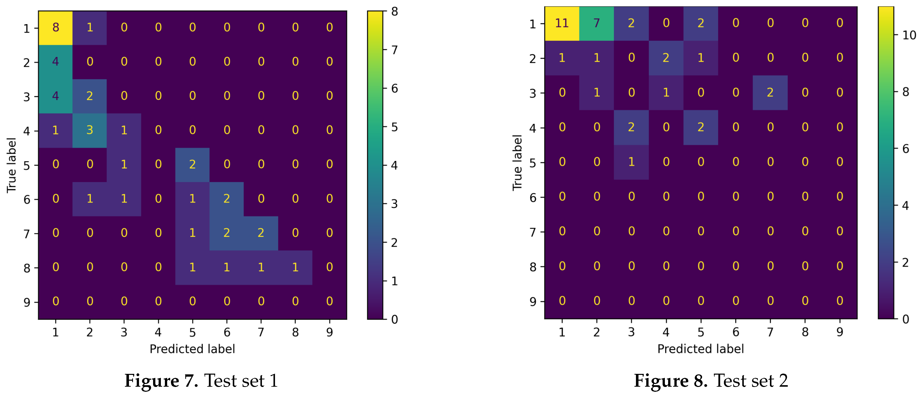
For a finer understanding of those results, we also report confusion matrices by assigning each predicted score to the closest integer to get classes.
The first test set yields satisfactory results. The points are mostly aligned along the main diagonal of the confusion matrix. The main issue is that the model tends to overall underestimate the yellow rust gravity, as evident from the lower triangular part of Figure 7. This issue probably arises from the scarcity of heavily diseased plots in the training dataset, with only 3 plots having a disease score of 9 (see Figure 3). Conversely, the model is struggling to generalise on the second test set. In particular, lower classes are often overrepresented, as visible in the upper triangular part in Figure 8. This hinders the capabilities of the model to yield good results.
Figure 9.
Confusion matrices obtained by rounding the model’s outputs to the nearest integer, for Test 1 (a) and Test 2 (b).
Figure 9.
Confusion matrices obtained by rounding the model’s outputs to the nearest integer, for Test 1 (a) and Test 2 (b).
3.3. Architectural Ablation Study
In this section, we perform an ablation study to support our architectural choices in our base model. We are interested in testing for the following components which we ablate in Table A2 and 6:
- spectral attention: on the line "no heads", we remove the spectral selection and simply feed all bands and indices directly to the spatial processor. We also report results for feeding only RGB directly to the spatial processor on the line "RGB only".
- chunk attention: on the line "with chunking", we perform chunking along the width in the spatial processor, and the associated spatial attention, with 3 chunks.
- feature selection: on the line "no feature selector", we remove the feature selector layer and feed the concatenated features from the chunk attention directly to the LSTM.
- time attention: on the line "time average", we replace time attention with an average of all the outputs of the LSTM along the time dimension. On the line "time concatenation", we replace time attention with a concatenation of all the outputs of the LSTM along the time dimension.
Each of the above investigation is conducted independently, by removing the corresponding component from the base model all other things being equal. We report our results in Table 6.
Table 6.
Results obtained with variants of the base model. Each line shows an independent variant obtained by modifying the base model as described in Section 3.3.
Table 6.
Results obtained with variants of the base model. Each line shows an independent variant obtained by modifying the base model as described in Section 3.3.
| Variant | Data split | MSE | MAD | Top-1 Accuracy | Top-2 Accuracy | Top-3 Accuracy |
| base model | Validation | 1.20[0.74,1.83] | 0.84[0.69,1.00] | 0.38[0.27,0.50] | 0.74[0.63,0.84] | 0.87[0.79,0.94] |
| no heads | Validation | 1.52 [0.88;2.41] | 0.93 [0.76;1.19] | 0.35 [0.25;0.46] | 0.68 [0.57;0.78] | 0.85 [0.76;0.93] |
| RGB only | Validation | 1.38 [0.90;2.00] | 0.90 [0.73;1.09] | 0.36 [0.25;0.47] | 0.71 [0.60;0.81] | 0.86 [0.78;0.93] |
| no feature selector | Validation | 1.48 [0.95;2.12] | 0.93 [0.74;1.12] | 0.37 [0.26;0.47] | 0.68 [0.56;0.79] | 0.82 [0.73;0.90] |
| time average | Validation | 1.44 [0.90;2.07] | 0.92 [0.76;1.10] | 0.34 [0.25;0.46] | 0.67 [0.56;0.78] | 0.83 [0.74;0.91] |
| time concatenation | Validation | 1.64 [0.97;2.47] | 0.96 [0.77;1.17] | 0.35 [0.24;0.46] | 0.68 [0.56;0.78] | 0.82 [0.71;0.90] |
As shown in Table 6, the architecture of the base model demonstrates superior - although not in a statistically significant way with regards to our validation set - performance compared to its variants across all examined metrics. Notable observations include:
- Overall performance: the base model consistently but not statistically significantly outperforms all ablated variants in terms of all the considered metrics, as visible in Table 6. This result requires confirmation from future validation experiments since the Test results did not prove to be statistically descriptive, being too small (see Table A2).
- Impact of spatial attention: extensive experimentation reveals that the inclusion of the spatial attention mechanism results in slightly worse performance compared to its absence. Despite this, the additional robustness and interpretability introduced by the spatial attention might justify minor performance drops.
- RGB performance: It is striking that the RBG solution offers comparable results to the multispectral one. The main advantage is that RGB solutions are economically more viable than MS approaches.
This ablation study highlights the contribution of each component to the regression problem, emphasising the importance of the overall model architecture in achieving optimal performance.
3.4. Producing Insights for Remote Phenotyping Practices
One of our main goals in this study is not only to develop a phenotype-agnostic model and to optimise it for yellow rust phenotyping but also to pave the way for more usable and scalable research and solutions for remote phenotyping. For this reason, the TriNet architecture incorporates several components chosen for their explainability. Although it is generally true that restricting deep architectures to be explainable can hinder their capabilities, in many cases it can serve as a powerful inductive bias and actually improve the results as explained in [64]. In plant breeding, works such as [65,66,67] have successfully used explainable components as inductive biases to facilitate training. In our case, we have seen in Section 3.3 that attention on spatial chunks reduces the model’s performance but that our other explainable components have a positive impact.
In this section, we train a new model with different parameters to optimise the insights we can gain from the model, as opposed to optimising for the model’s performance. In practice, because our base model already uses our other interpretability modules, this simply amounts to turning the spatial chunking back on and running the model with chunks in our spatial processor.
The obtained model’s results can be found in Table 7.
The information in the three heads can be recombined to obtain a ranking of the most important channels in the input images. This is done considering the average of the different channel across the three heads. Figure 11 presents the channels’ aggregate importance.
We show in Figure 10 and Figure 12 how the attention weights of the two layers of interest behave as the training progresses. The model selects the EVI, GNDVI and red bands and indices, which we further validate in Section 3.5 and comment in Section 4.2. In terms of time steps, it selects the 6th, 7th and 5th time steps. For example, the fourth UAV acquisition could likely have been omitted in a lower-resource project. This does not mean that the acquisition was incorrectly performed, but rather, in our interpretation, that it contains redundant information already captured by other flights. We further validate these intuitions in Section 3.5 and comment in Section 4.3.
Figure 10.
Evolution of the weights for each of the 3 attention heads (columns) in the spectral processor during training, after softmax. Even with no entropy regularisation, each head learns to prioritise inputs bands (line 1) and indices (line 2) differently over the course of the training run. Line 3 shows the final rankings in each head.
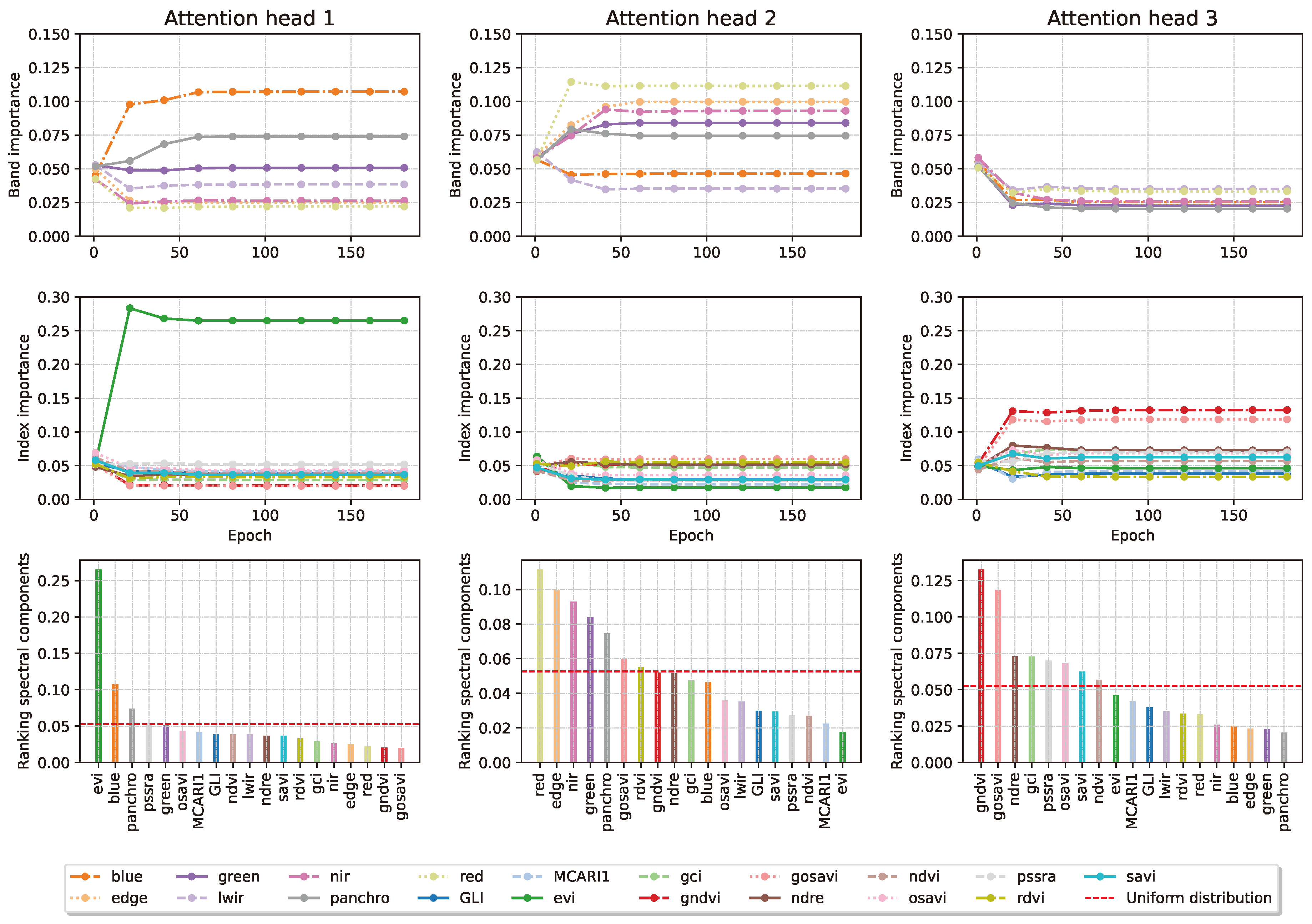
Figure 11.
Averaged evolution of the weights for the 3 attention heads in the spectral processor during training, after softmax. The importance of the bands is acquired every 20 epochs. EVI, GNDVI and the Red band come out on top of this analysis.
Figure 11.
Averaged evolution of the weights for the 3 attention heads in the spectral processor during training, after softmax. The importance of the bands is acquired every 20 epochs. EVI, GNDVI and the Red band come out on top of this analysis.
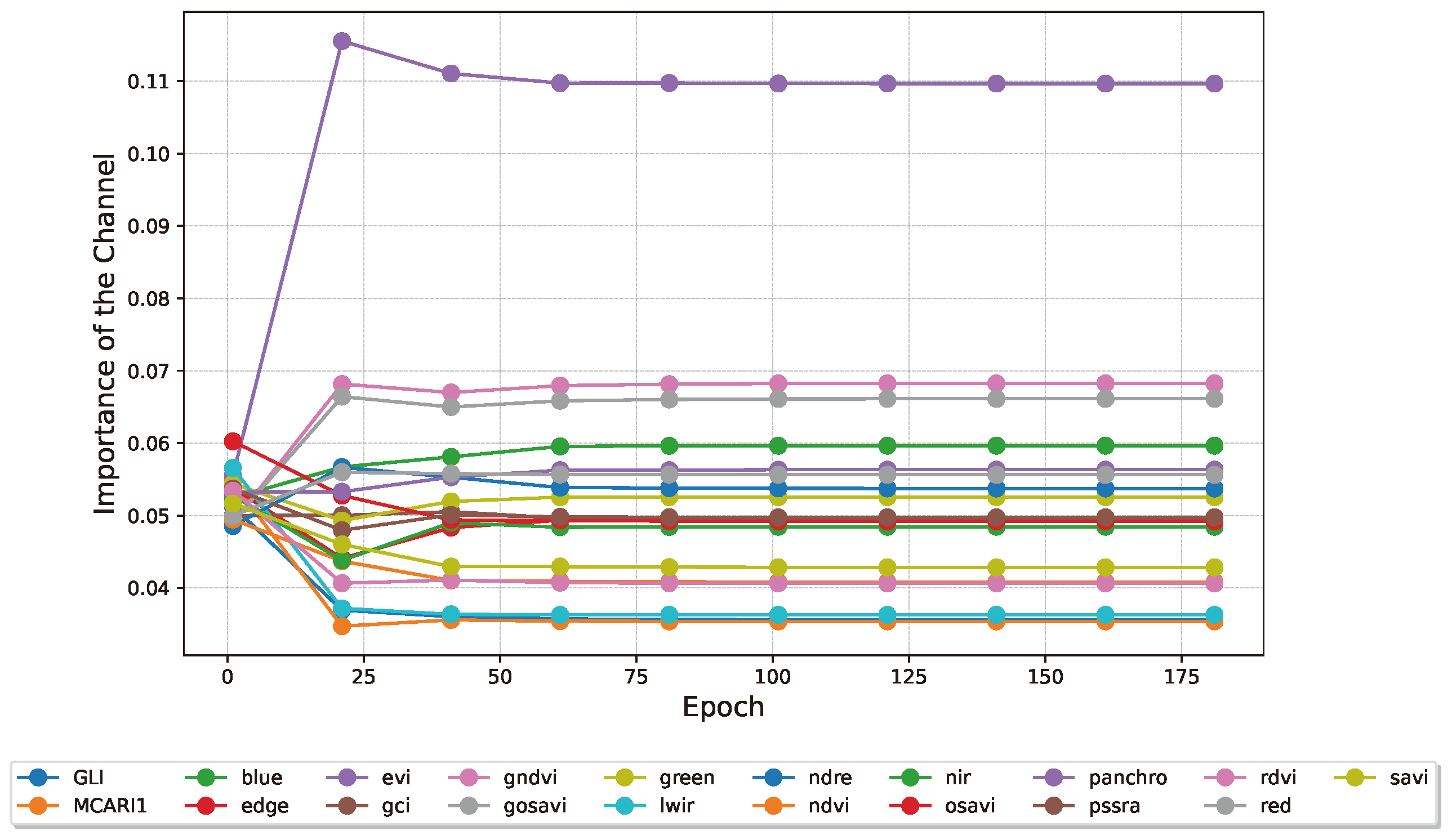
Figure 12.
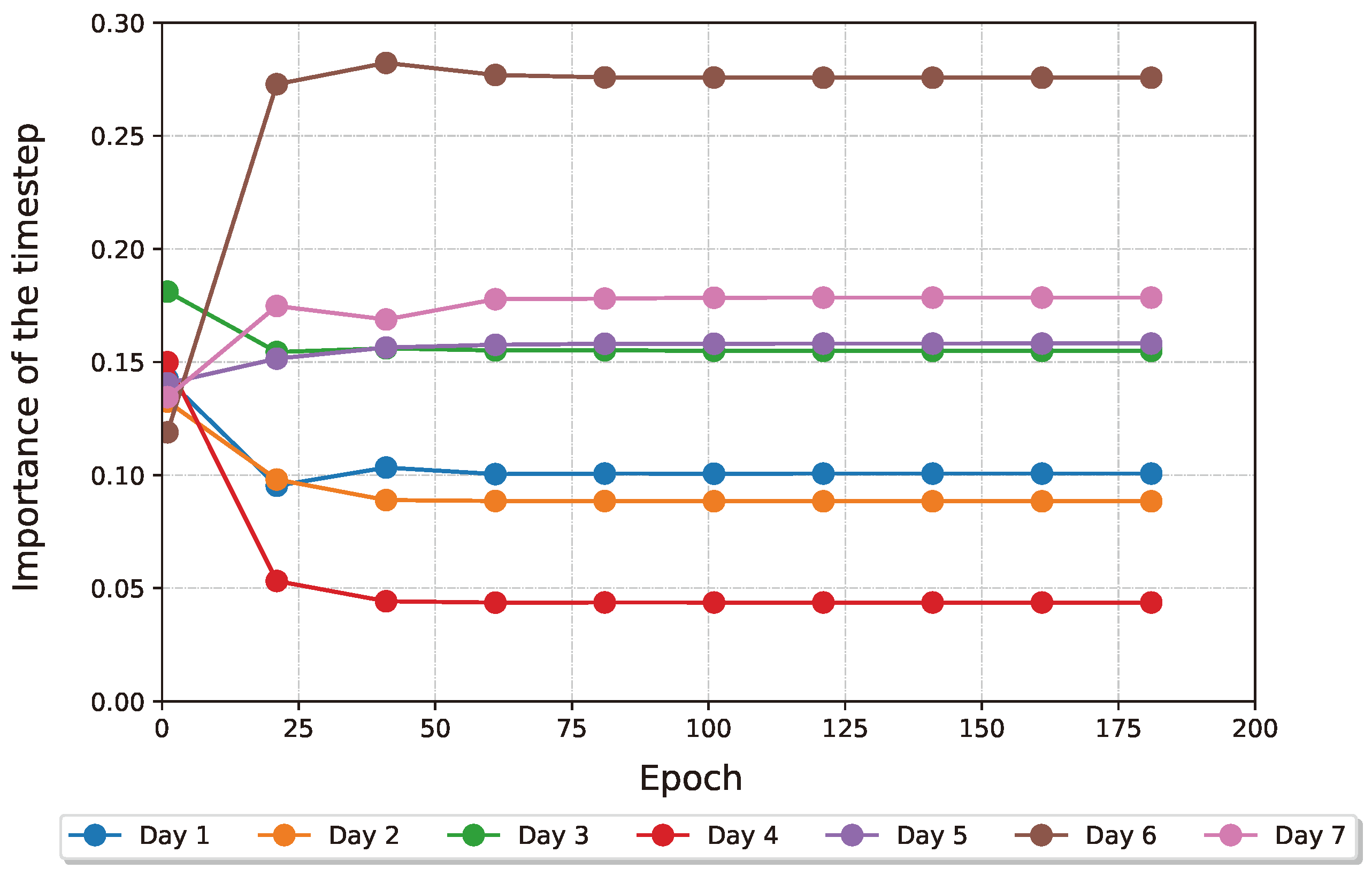
Evolution of the attention weights in the temporal processor during training, after softmax. Using a high enough entropy regularisation forces the layer to be more selective. The 6th, 7th and 5th time steps come out on top of this analysis.
Figure 12.
Evolution of the attention weights in the temporal processor during training, after softmax. Using a high enough entropy regularisation forces the layer to be more selective. The 6th, 7th and 5th time steps come out on top of this analysis.
It is important to notice that the best performing model does not perform spatial attention, since the number of chunks of the model is one. We want to propose it a tradeoff between the model’s additional roboustness and the model’s performance. In fact the base model (see Table 5, 1 chunk) outperforms the most explainable model (see Table 7, 3 chunks) in all the considered metrics metrics. Here, in virtue of the scalability that we seek, we devise two modes of the same problem to see whether
In the next section, we verify that these indices and time steps are indeed good predictors for yellow rust phenotyping, therefore proving the capacity of our interpretable components to yield actionable insights.
3.5. Insights Validation
In this section, we conduct experiments to validate the insights indicated in Section 3.4. There are two main insights we want to validate: the model’s selected bands and indices, and the model’s selected time step.
To validate the selected bands, we propose to train a model, without spectral processor, taking the bands selected automatically by TriNet as input to the spatial processor. We then compare it with models using random selections of bands instead, to show that our explainable layer has converged to a sensible choice without explicit intervention. Those results can be found in Table 8.
Our results indicate that the selected bands achieve performance comparable to the full model within a 90% confidence interval. Notably, the model using our selected bands and timesteps outperforms random selections in key metrics, including top-3 accuracy, where it surpasses 29 out of 30 random experiments. We provide further discussion on these findings in Section 4.2.
To validate the selected time steps, we propose to train a model, without temporal processor, taking as input the time step selected by TriNet. We then compare it with models using random time steps instead, to show that our explainable layer has converged to a sensible choice without explicit intervention. Those results can be found in Table 9 for the validation set and in Table A3 for the two test sets.
Our results indicate that the selected time steps achieve a performance comparable to the full model within a 90% confidence interval, with a top-3 accuracy of 0.83. In Table 9 we also present a comparison with a random subset of UAV acquisition dates composing the training dataset. When it comes to our metric of choice, top-3 accuracy, the selected time steps perform better than 39 out of 39 random experiments. We comment on those results further in Section 4.3.
4. Discussion
In our study, we propose to improve the scalability of automated phenotyping via multispectral imagery captured by a UAV. Given its importance in agriculture, we chose yellow rust as the phenotype to tackle (see Section 1). Still, the model can also be applied to different phenotypes as the target. We approach this problem from several angles:
- recommended scoring methods have a high granularity from 1 to 9, contrary to most existing published methods. This higher granularity is an advantage to scale algorithms to different purposes (which might need different target resolutions) or different countries (which might employ different scales), therefore we stick to this more expressive scale for our ground truth targets;
- current methods often achieve very high phenotyping performance by using very small GSDs. We propose to make them more scalable by analysing the performance of algorithms working from 60 metres-high data and a GSD of 2.5cm for the multispectral bands;
- some methods, including ours, use time series or a large variety of spectral bands which require more resources to deploy. We train our model to contain explainability components to optimise the number of bands and flights we need;
- we endeavour to make models more explainable to make them more robust and reliable, and explore the trade-offs with model performance they sometimes present.
In what follows, we analyse these objectives and discuss our contributions with respect to the state-of-the-art.
4.1. Using Low Spatial Resolution and High Target Resolution.
The approach proposed in this paper aims to achieve greater scalability in remote phenotyping across multiple aspects. At the proposed flight height, a flight to capture all of our 1025 test fields takes around 7 minutes, which can be achieved without changing the battery, and the resulting data after the preparation process described takes under 6GB of disk space. These numbers are unfortunately not reported in prior literature, preventing us from an in-depth analysis. Given the differences in GSD, we can nevertheless assume that our setup requires much less storage space and computing power for processing per square metre of field. Similarly, we assume that flights at lower altitude would require higher flight times for equivalent area sizes with a more than proportional increase due to the need to ensure sufficient overlap for photogrammetric reconstruction and the need to change batteries more frequently (a very time-consuming operation).
We also claim that the existing literature is very hard to compare to due to the lack of granularity in the target definition they use, which is at odds with existing standards in the field such as those provided by the AGES, the Federal Plant Variety Office in Germany, or the Cobb scale. Collapsing detailed measurement scales to 2 or 3 classes makes the reported results ambiguous and difficult to generalise, re-use, reproduce and validate. It is also at odds with the needs of plant breeders, who consequently cannot fully leverage the potential of these new technologies.
We finally report classification accuracies for phenotyping performed at an altitude of 60m, corresponding to 2.5 cm/pixel. We also use the more robust scale provided by the AGES and accordingly, score yellow rust between 1 and 9. We show that this more scalable setup, although more challenging from an ML perspective, still achieves promising results. Specifically, we achieve 38% of accuracy out of 9 classes for the validation dataset and 33% and 35% respectively on test set 1 and test set 2 (See Table 5). When using more practically oriented metrics which better reflect the plant breeders’ needs and are easier to compare with the 2- or 3-class case, our results further jump to 0.74% for the validation score and 0.55 and 0.57 respectively for test set 1 and 2 for top-2 accuracy, and 0.87% for validation and 0.67% and 0.70% respectively for test set 1 and test set 2 for top-3 accuracy. The scores on the test set are generally lower, which we attribute to a general lack of data which posed serious challenges to the generalisation capabilities of the model. Nevertheless, in the context of plant breed selection, a top-3 accuracy in the range of 0.7 proves to be sufficient especially in early trials of breed selection, when time is the limiting factor of this application. New iterations of these experiments with additional data are an interesting avenue for future research.
Despite the potential loss of fine details with lower spatial resolution, we thus developed robust algorithms to extract meaningful features from coarser data. To ensure the impact of our architectural choices on our results, we conducted an architectural ablation study, evaluating various model variants. This study systematically analysed the impact of different components on performance, incorporating explainability components to optimise the number of spectral bands and flights, while maintaining high target resolution. Our ablation study results, summarised in Table A2 and 6, indicate that all modified variants perform worse than our chosen model.
These findings confirm that our base model, even with lower spatial resolution and higher target resolution, maintains high accuracy and robustness, making it more suitable for large-scale deployment. This ensures our phenotyping algorithms are adaptable by design to different agricultural practices and set-ups, providing a scalable, efficient solution for yellow rust phenotyping. However, in this study, we do compensate for our lack of spatial resolution with increased spectral and temporal resolution. In the next sections, we analyse our results in terms of spectral and temporal efficiency and suggest future directions to find optimal trade-offs between the three dimensions.
4.2. Optimising Bands for Cheaper Cameras and Drones
An argument can be made for reducing the cost of cameras and drones, thereby enhancing scalability, based on the decent results achievable using only RGB imaging. Our study demonstrates that the "RGB only" variant performs competitively, achieving a top-3 accuracy ranging from 0.73 to 0.80 across different tests. This level of accuracy is comparable to 2- and 3-class studies in the literature, where similar methods have shown effective performance in distinguishing between classes.
TriNet uses 5 multispectral bands, the panchromatic and LWIR band as well as 13 indices as input to compute yellow rust scores, which is significantly more than a simple RGB input. However, our model is designed to select the most useful bands and indices at an early stage and in an interpretable manner. In Table 8, we show that training a model with the selected bands and indices as input (, and ) reaches a top-3 accuracy of 0.84% on the validation and 0.66% and 0.71 % respectively on test set 1 and 2 (see Table A4). across our tests. This is not only better than the 95th percentile of experiments using random bands and indices but also on par with our base model which has access to all bands. These indices would require RGB input as well and the band to be computed. Therefore, these results do not only pinpoint a minimal set of bands (, , , ) to achieve the best results but also quantify the added benefit of the band compared to traditional RGB cameras. Moreover, the model generalises well on the validation data using only RGB data as the training input (see Table 8). This poses significant economic upsides in planning a monitoring campaign since UAV equipped with RGB sensors only are significantly cheaper than a multispectral or hyperspectral sensor. Nevertheless, further research in this direction is necessary to assess whether this holds only for Yellow Rust monitoring or also generalises to other phenotypes. Yellow rust can be observed in the visible band, while the NIR band provides important insights for other phenotypes, for instance, the drought stress level or chlorophyll content [68].
These results highlight the potential for cost-effective phenotyping solutions. By using accessible and affordable RGB bands, researchers can improve scalability without significantly compromising performance. For higher accuracy, adding the NIR band provides quantifiable benefits. This approach supports broader adoption of phenotyping methods in agriculture and adapts to various operational contexts and resource constraints. Specifically, yellow rust signs are observable in the visible spectrum, but for phenotypes like water stress, the RGB spectrum alone may not suffice.
4.3. Optimising Time Steps for Easier Phenotyping Campaigns
Similarly to spectral resolution, time resolution is also an important source of cost when scaling phenotyping operations. Performing UAV flights on a regular basis can be a complex task, and the more time steps are required, the more brittle the overall process becomes. Indeed, UAVs require good weather, low wind speed, and can sometimes break and need repairs. As such, the number of time steps to acquire becomes a determining constraint for actual deployment of remote phenotyping technologies. We therefore make it a priority to study the importance of different time steps for TriNet.
TriNet uses 7 time steps, spaced out throughout the winter wheat’s life cycle. In the same way that it is designed to select input bands and indices, it is also designed to select the importance of input time steps in an interpretable way. In Table 9, we show that the best 2 timesteps (6 and 7) chosen by the time attention perform better than the 95th percentile of models trained with a random subsample of points, according to the top-3 accuracy. This accomplishment not only proves that the attention mechanism is effective in selecting the most meaningful dates inside the model, but also that it can be used to obtain domain information to schedule more effective and optimised UAV acquisition schedules. It is important to acknowledge that the last two time steps are also when yellow rust is more visible on the plants. Nevertheless, studying the importance coefficients given by the time attention can generate insights into the exact date and developmental stage when to start acquiring drone data for future UAV acquisition campaigns without hindering performance.
Therefore, we show that it is possible to optimise the time steps used by TriNet to significantly reduce the resource requirements associated to organising flight campaigns.
However, the study presented here is only preliminary. Indeed, in practical scenarios, it is difficult to plan when flights will be possible and when symptoms of yellow rust will appear. More broadly, different time steps might be optimal to study different phenotypes, and those optimal time steps would also depend on the growth stage of the wheat. For a truly scalable multi-temporal phenotyping to be deployed with the current weather-dependent technologies, more work should be done to train models able to leverage arbitrary input time steps to assess a given phenotype at arbitrary output time steps. Moreover, these models should be capable of estimating their own uncertainty when predicting a phenotype at a time step that is temporally remote from any available observation.
5. Conclusion
In this study, we address the challenge of scaling automated phenotyping using UAVs, focusing on yellow rust as the target phenotype. Our approach involves several innovative strategies to enhance scalability and performance, making our methodology applicable to various phenotypes and agricultural contexts.
First, we adopt a high granularity in-situ scoring method (1 to 9 scale) to accommodate different target resolutions and standards across countries, ensuring broader applicability and better alignment with plant breeders’ needs.
Second, we demonstrate that using lower spatial resolution (60m flight height and 2.5 cm GSD) significantly reduces the resources required for data acquisition, processing and storage, without severely compromising the prediction accuracy when compared to the most recent approaches reported in Table 1. This setup facilitates faster data acquisitions and lower operational costs, making large-scale phenotyping more feasible. Our framework shows that such higher-altitude flights constitute a relevant design space for phenotyping practices, and enable testing of various tradeoffs between spatial, spectral and temporal resolution. We therefore pave the way for future efforts to determine the Pareto frontier between those parameters and make phenotyping more scalable.
Third, we incorporate explainability components into our models, optimising the number of spectral bands and flights required. This not only improves model robustness and reliability but also helps identify the most relevant features, thus simplifying the deployment process.
Our results show that our model achieves promising performance even with lower spatial resolution and a high target resolution of 9 steps. Specifically, we attained top-3 accuracies of 0.87% for validation and 0.67% and 0.70% for test sets 1 and 2, respectively. These results underscore the effectiveness of our approach in balancing resource efficiency and phenotyping accuracy.
Future research should focus on further optimising the trade-offs between spatial, spectral and temporal resolutions to enhance the applicability and efficiency of phenotyping technologies in diverse agricultural settings across various species and phenotypes. We also deem important the creation of a time-agnostic model which would be independent of a given set of acquisition dates. Another cruicial direction for future research is a comprehensive study of the portability of TriNet to different phenotypes, such as the plant’s water status or yield content. Our encouraging results with yellow rust disease scoring show that the physiological status of the plant correlates with the latent space feature representation. Therefore, avenues are open to leverage transfer learning to phenotype other wheat diseases such as stripe rust and brown rust, or even different traits.
Table 10.
Dates of data acquisition and growth stages of winter wheat.
| Date of the flight | Growth Stage |
|---|---|
| March 22, 2023 | Stem Elongation |
| April 18, 2023 | Stem Elongation |
| April 27, 2023 | Booting |
| May 15, 2023 | Heading |
| May 24, 2023 | Flowering |
| June 5, 2023 | Milk Development |
| June 14, 2023 | Dough Development |
Author Contributions
Conceptualisation, Lorenzo Beltrame, Jules Salzinger, Lukas J. Koppensteiner, Phillipp Fanta-Jende; Methodology, Lorenzo Beltrame, Jules Salzinger, Lukas J. Koppensteiner, Phillipp Fanta-Jende; Data curation, Lorenzo Beltrame, Lukas J. Koppensteiner; Visualisation, Lorenzo Beltrame; Software, Lorenzo Beltrame, Jules Salzinger; Validation, Jules Salzinger, Lorenzo Beltrame; Investigation, Lorenzo Beltrame, Jules Salzinger; Writing—original draft preparation, Lorenzo Beltrame, Lukas J. Koppensteiner, Jules Salzinger; Writing—review and editing, Jules Salzinger, Phillipp Fanta-Jende; Supervision, Jules Salzinger, Phillipp Fanta-Jende. All authors have read and agreed to the published version of the manuscript.
Funding
The author(s) declare financial support was received for the research, authorship, and/or publication of this article. This review has been conducted in the frame of the d4agrotech initiative (www.d4agrotech.at), in which the project ‘WheatVIZ’ (WST3-F-5030665/018-2022) received funding from the Government of Lower Austria.
Data Availability Statement
The data supporting the reported results, including the in-situ scoring data, are not published alongside this paper. However, we aim to make this data available to the public very soon, along with our latest data acquisitions of 2024. Detailed information regarding the data release will be provided in subsequent updates. For further inquiries or to request early access, please contact the corresponding author.
Acknowledgments
We would like to thank all the personnel of the Edelhof seed breeding institute and facility as well as Felix Bruckmüller for the UAV-based multispectral data acquisition. We also want to thank Maria Eva Molin for the supervision over the WheatVIZ project.
Conflicts of Interest
The authors declare no conflicts of interest.
Abbreviations
The following abbreviations are used in this manuscript:
| AGES | Austrian Agency for Health and Food Safety GmbH |
| COMM. | Commercial cultivars used in our test sets |
| GCP | Ground Control Point |
| GSD | Ground Sampling Distance |
| LWIR | Longwave Infrared |
| MAD | Mean Absolute Deviation |
| ML | Machine Learning |
| MSE | Mean Squared Error |
| NIR | Near Infrared |
| RGB | Red Green Blue |
| UAV | Unmanned Aerial Vehicle |
| Various index abbreviations | see Table 3 |
Appendix A
The number of attention heads chosen corresponds to the number of channels in the feature maps after spectral attention (see 5). Since ResNet-34 is trained on RGB images, we subdivide the feature maps into multiple three-channel multispectral cubes along the channel dimension. To achieve this, we use the following heuristic: if the number of channels is divisible by 3, we divide them along the channel dimension. If not, we apply a convolution to increase the number of remaining channels to 3. After this processing, each multispectral cube input to ResNet-34 requires renormalisation, as shown in Table A1.
Table A1.
Mean and standard deviation values specified by ResNet for each channel, originally for RGB bands but applied here to multispectral cubes.
Table A1.
Mean and standard deviation values specified by ResNet for each channel, originally for RGB bands but applied here to multispectral cubes.
| Channel 1 (R) | Channel 2 (G) | Channel 3 (B) | |
| Mean | 0.485 | 0.456 | 0.406 |
| Standard Deviation | 0.229 | 0.224 | 0.225 |
Appendix B
Table A2.
Results obtained with variants of the base model. Each line shows an independent variant obtained by modifying the base model as described in Section 3.3. Since the test set are small the confidence interval with a 90% coverage probability are large. Therefore no statistically solid insight can be extracted from these test set. Further work is ought to tackle this issue.
| Variant | Data split | MSE | MAD | Top-1 Accuracy | Top-2 Accuracy | Top-3 Accuracy |
| Base model | Test 1 | 2.51 [1.04,4.64] | 1.23 [0.75,1.80] | 0.31 [0.07,0.57] | 0.52 [0.24,0.79] | 0.67 [0.42,0.88] |
| Test 2 | 2.69 [0.75,5.73] | 1.20 [0.67,1.87] | 0.35 [0.08,0.62] | 0.54 [0.24,0.81] | 0.70 [0.41,0.95] | |
| no heads | Test 1 | 2.40 [0.88;4.52] | 1.19 [0.68;1.74] | 0.31 [0.10;0.56] | 0.54 [0.26;0.79] | 0.73 [0.47;0.93] |
| Test 2 | 1.97 [0.72;3.57] | 1.10 [0.63;1.67] | 0.39 [0.14;0.68] | 0.61 [0.33;0.89] | 0.66 [0.38;0.90] | |
| RGB only | Test 1 | 2.50 [0.87;5.06] | 1.23 [0.75;1.78] | 0.24 [0.04;0.48] | 0.49 [0.22;0.76] | 0.73 [0.49;0.93] |
| Test 2 | 1.34 [0.55;2.46] | 0.96 [0.64;1.36] | 0.25 [0.03;0.50] | 0.61 [0.33;0.89] | 0.80 [0.57;1.00] | |
| no feature selection | Test 1 | 2.38 [0.96;4.63] | 1.22 [0.78;1.75] | 0.32 [0.10;0.58] | 0.51 [0.24;0.76] | 0.76 [0.51;0.95] |
| Test 2 | 2.15 | 1.07 [0.64;1.72] | 0.42 [0.14;0.69] | 0.64 [0.36;0.89] | 0.72 [0.44;0.94] | |
| time average | Test 1 | 2.73 [0.93;5.34] | 1.26 [0.75;1.87] | 0.37 [0.13;0.63] | 0.48 [0.23;0.76] | 0.71 [0.44;0.93] |
| Test 2 | 1.57 [0.71;2.80] | 1.07 [0.72;1.47] | 0.22 [0.03;0.49] | 0.53 [0.25;0.81] | 0.78 [0.53;0.97] | |
| time concatenation | Test 1 | 2.58 [0.66;5.75] | 1.16 [0.64;1.76] | 0.34 [0.10;0.60] | 0.56 [0.28;0.82] | 0.82 [0.61;0.98] |
| Test 2 | 1.69 [0.61;3.11] | 1.02 [0.62;1.47] | 0.27 [0.04;0.54] | 0.61 [0.32;0.87] | 0.77 [0.51;0.98] |
Table A3.
Results obtained with variants of the base model. Line 1 is the base model presented in Table 5. Line 2 is the same architecture using only the best 2 selected timesteps: 6 and 7. Lines 3, 4 and 5 show the 5th, 50th and 95th percentiles of 39 independent models trained on random sets of three bands.
| Variant | Data split | MSE | MAD | Top-1 Accuracy | Top-2 Accuracy | Top-3 Accuracy |
| Base model | Test 1 | 2.51 [1.04,4.64] | 1.23 [0.75,1.80] | 0.31 [0.07,0.57] | 0.52 [0.24,0.79] | 0.67 [0.42,0.88] |
| Test 2 | 2.69 [0.75,5.73] | 1.20 [0.67,1.87] | 0.35 [0.08,0.62] | 0.54 [0.24,0.81] | 0.70 [0.41,0.95] | |
| Timestep 6 and 7 | Test 1 | 3.03 [1.33,5.47] | 1.39 [0.86,1.92] | 0.24 [0.05,0.50] | 0.45 [0.21,0.73] | 0.67 [0.42,0.90] |
| Test 2 | 2.40 [0.86,4.43] | 1.22 [0.73,1.81] | 0.11 [0.00,0.30] | 0.59 [0.32,0.86] | 0.70 [0.43,0.92] | |
| 5th percentile | Test 1 | 7.59 [3.34,13.33] | 2.21 [1.43,3.07] | 0.10 [0.00,0.26] | 0.22 [0.05,0.45] | 0.45 [0.20,0.71] |
| Test 2 | 2.44 [1.14,5.52] | 1.25 [0.87,1.82] | 0.08 [0.00,0.27] | 0.22 [0.03,0.47] | 0.68 [0.41,0.92] | |
| 50th percentile | Test 1 | 3.25 [1.18,6.58] | 1.41 [0.89,2.06] | 0.17 [0.01,0.38] | 0.46 [0.21,0.73] | 0.64 [0.37,0.87] |
| Test 2 | 1.63 [0.61,2.96] | 1.04 [0.67,1.50] | 0.14 [0.00,0.35] | 0.59 [0.32,0.86] | 0.78 [0.54,0.97] | |
| 95th percentile | Test 1 | 2.30 [0.77,4.70] | 1.15 [0.71,1.75] | 0.33 [0.09,0.59] | 0.52 [0.27,0.79] | 0.71 [0.45,0.94] |
| Test 2 | 1.23 [0.42,2.11] | 0.88 [0.54,1.29] | 0.35 [0.09,0.62] | 0.75 [0.47,0.94] | 0.86 [0.65,1.00] |
Table A4.
Results obtained with variants of the base model. Line 1 is the base model presented in Table 5. Line 2 is the same architecture using only the best 3 selected bands and indices: EVI, red and GNDVI. Line 3 is the same architecture using only the Red, Green and Blue bands. Lines 4, 5 and 6 show the 5th, 50th and 95th percentiles of 30 independent models trained on random sets of three bands.
| Variant | Data split | MSE | MAD | Top-1 Accuracy | Top-2 Accuracy | Top-3 Accuracy |
| Base model | Test 1 | 2.51 [1.04,4.64] | 1.23 [0.75,1.80] | 0.31 [0.07,0.57] | 0.52 [0.24,0.79] | 0.67 [0.42,0.88] |
| Test 2 | 2.69 [0.75,5.73] | 1.20 [0.67,1.87] | 0.35 [0.08,0.62] | 0.54 [0.24,0.81] | 0.70 [0.41,0.95] | |
| EVI, red, GNDVI | Test 1 | 2.51 (0.95,4.87) | 1.23 (0.74,1.81) | 0.31 (0.10,0.56) | 0.52 (0.26,0.81) | 0.67 (0.42,0.88) |
| Test 2 | 1.20 (0.66,1.90) | 2.69 (0.69,5.62) | 0.35 (0.09,0.64) | 0.54 (0.26,0.81) | 0.70 (0.43,0.95) | |
| RGB only | Test 1 | 2.93 [1.17;5.62] | 1.33 [0.81;1.93] | 0.24 [0.04;0.48] | 0.49 [0.22;0.76] | 0.73 [0.49;0.93] |
| Test 2 | 1.72 [0.56;3.74] | 1.05 [0.61;1.52] | 0.25 [0.03;0.50] | 0.61 [0.33;0.89] | 0.80 [0.57;1.00] | |
| 5th percentile | Test 1 | 2.30 [0.77;4.70] | 1.15 [0.71;1.75] | 0.10 [0.00;0.26] | 0.22 [0.05;0.45] | 0.45 [0.20;0.71] |
| Test 2 | 1.23 [0.42;2.11] | 0.88 [0.54;1.29] | 0.08 [0.00;0.27] | 0.22 [0.03;0.47] | 0.68 [0.41;0.92] | |
| 50th percentile | Test 1 | 3.25 [1.18;6.58] | 1.41 [0.89;2.06] | 0.17 [0.01;0.38] | 0.46 [0.21;0.73] | 0.64 [0.37;0.87] |
| Test 2 | 1.63 [0.61;2.96] | 1.04 [0.67;1.50] | 0.14 [0.00;0.35] | 0.59 [0.32;0.86] | 0.78 [0.54;0.97] | |
| 95th percentile | Test 1 | 7.59 [3.34;13.33] | 2.21 [1.43;3.07] | 0.33 [0.09;0.59] | 0.52 [0.27;0.79] | 0.71 [0.45;0.94] |
| Test 2 | 2.44 [1.14;5.52] | 1.25 [0.87;1.82] | 0.35 [0.09;0.62] | 0.75 [0.47;0.94] | 0.86 [0.65;1.00] |
References
- Ray, D.K.; Ramankutty, N.; Mueller, N.D.; West, P.C.; Foley, J.A. Recent patterns of crop yield growth and stagnation. Nature Communications 2012, 3, 1293. [CrossRef]
- Ray, D.K.; Mueller, N.D.; West, P.C.; Foley, J.A. Yield Trends Are Insufficient to Double Global Crop Production by 2050. PLoS ONE 2013, 8, e66428. [CrossRef]
- Feng, L.; Chen, S.; Zhang, C.; Zhang, Y.; He, Y. A comprehensive review on recent applications of unmanned aerial vehicle remote sensing with various sensors for high-throughput plant phenotyping. Computers and Electronics in Agriculture 2021, 182, 106033. [CrossRef]
- Chen, W.; Wellings, C.; Chen, X.; Kang, Z.; Liu, T. Wheat stripe (yellow) rust caused by P uccinia striiformis f. sp. tritici. Molecular Plant Pathology 2014, 15, 433–446. [CrossRef]
- Stubbs, R., Stripe Rust; Elsevier, 1985; pp. 61–101. [CrossRef]
- Wan, A.M.; Chen, X.M.; He, Z.H. Wheat stripe rust in China. Australian Journal of Agricultural Research 2007, 58, 605. [CrossRef]
- Chen, X.; Kang, Z., Eds. Stripe Rust; Springer Netherlands, 2017. [CrossRef]
- Zadoks, J.C.; Rijsdijk, F.; others. Agro-ecological atlas of cereal growing in Europe. Vol. III. Atlas of cereal diseases and pests in Europe.; Centre for Agricultural Publishing and Documentation (Pudoc), 1984.
- Chen, X.; Kang, Z., Eds. Stripe Rust; Springer Netherlands, 2017. [CrossRef]
- Chen, X. Pathogens which threaten food security: Puccinia striiformis, the wheat stripe rust pathogen. Food Security 2020, 12, 239–251. [CrossRef]
- Araus, J.L.; Cairns, J.E. Field high-throughput phenotyping: The new crop breeding frontier. Trends in Plant Science 2014, 19, 52–61. [CrossRef]
- Radoglou-Grammatikis, P.; Sarigiannidis, P.; Lagkas, T.; Moscholios, I. A compilation of UAV applications for precision agriculture. Computer Networks 2020, 172, 107148. [CrossRef]
- Delavarpour, N.; Koparan, C.; Nowatzki, J.; Bajwa, S.; Sun, X. A Technical Study on UAV Characteristics for Precision Agriculture Applications and Associated Practical Challenges. Remote Sensing 2021, 13, 1204. [CrossRef]
- Gracia-Romero, A.; Kefauver, S.C.; Fernandez-Gallego, J.A.; Vergara-Díaz, O.; Nieto-Taladriz, M.T.; Araus, J.L. UAV and Ground Image-Based Phenotyping: A Proof of Concept with Durum Wheat. Remote Sensing 2019, 11, 1244. [CrossRef]
- Moshou, D.; Bravo, C.; West, J.; Wahlen, S.; McCartney, A.; Ramon, H. Automatic detection of ‘yellow rust’ in wheat using reflectance measurements and neural networks. Computers and Electronics in Agriculture 2004, 44, 173–188. [CrossRef]
- Kukreja, V.; Kumar, D. Automatic Classification of Wheat Rust Diseases Using Deep Convolutional Neural Networks. IEEE, 2021, pp. 1–6. [CrossRef]
- Koc, A.; Odilbekov, F.; Alamrani, M.; Henriksson, T.; Chawade, A. Predicting yellow rust in wheat breeding trials by proximal phenotyping and machine learning. Plant Methods 2022, 18, 30. [CrossRef]
- Mi, Z.; Zhang, X.; Su, J.; Han, D.; Su, B. Wheat Stripe Rust Grading by Deep Learning With Attention Mechanism and Images From Mobile Devices. Frontiers in Plant Science 2020, 11. [CrossRef]
- Tang, Z.; Wang, M.; Schirrmann, M.; Dammer, K.H.; Li, X.; Brueggeman, R.; Sankaran, S.; Carter, A.H.; Pumphrey, M.O.; Hu, Y.; Chen, X.; Zhang, Z. Affordable High Throughput Field Detection of Wheat Stripe Rust Using Deep Learning with Semi-Automated Image Labeling. Computers and Electronics in Agriculture 2023, 207, 107709. [CrossRef]
- Zhang, X.; Han, L.; Dong, Y.; Shi, Y.; Huang, W.; Han, L.; González-Moreno, P.; Ma, H.; Ye, H.; Sobeih, T. A Deep Learning-Based Approach for Automated Yellow Rust Disease Detection from High-Resolution Hyperspectral UAV Images. Remote Sensing 2019, 11, 1554. [CrossRef]
- Nguyen, C.; Sagan, V.; Skobalski, J.; Severo, J.I. Early Detection of Wheat Yellow Rust Disease and Its Impact on Terminal Yield with Multi-Spectral UAV-Imagery. Remote Sensing 2023, 15, 3301. [CrossRef]
- Olson, D.; Anderson, J. Review on unmanned aerial vehicles, remote sensors, imagery processing, and their applications in agriculture. Agronomy Journal 2021, 113, 971–992. [CrossRef]
- Alzubaidi, L.; Zhang, J.; Humaidi, A.J.; Al-Dujaili, A.; Duan, Y.; Al-Shamma, O.; Santamaría, J.; Fadhel, M.A.; Al-Amidie, M.; Farhan, L. Review of deep learning: Concepts, CNN architectures, challenges, applications, future directions. Journal of Big Data 2021, 8, 53. [CrossRef]
- Su, J.; Liu, C.; Coombes, M.; Hu, X.; Wang, C.; Xu, X.; Li, Q.; Guo, L.; Chen, W.H. Wheat yellow rust monitoring by learning from multispectral UAV aerial imagery. Computers and Electronics in Agriculture 2018, 155, 157–166. [CrossRef]
- Peterson, R.F.; Campbell, A.B.; Hannah, A.E. A DIAGRAMMATIC SCALE FOR ESTIMATING RUST INTENSITY ON LEAVES AND STEMS OF CEREALS. Canadian Journal of Research 1948, 26c, 496–500. [CrossRef]
- McNeal, F.; Konzak, C.; Smith, E.; Tate, W.; Russel, T. A uniform system for recording and processing cereal research data; Agricultural Research Service, United States Department of Agriculture, 1971.
- McIntosh, R.; Wellings, C.R.; Park, R.F. Wheat Rusts: An Atlas of Resistance Genes. 1995.
- Mallard, S.; Gaudet, D.; Aldeia, A.; Abelard, C.; Besnard, A.L.; Sourdille, P.; Dedryver, F. Genetic analysis of durable resistance to yellow rust in bread wheat. Theoretical and Applied Genetics 2005, 110, 1401–1409. [CrossRef]
- Edelhof, S. Saatzucht Edelhof. https://www.bing.com/search?pglt=43&q=saatzuch+edelhof&cvid=015470d5ca97404a93bde7943e59cf4c&gs_lcrp=EgZjaHJvbWUyBggAEEUYOTIGCAEQABhA0gEINDMxNmowajGoAgiwAgE&FORM=ANNTA1&PC=U531, 2024. Accessed: May 2, 2024.
- Camera, A.P. Altum-PT Camera. https://ageagle.com/drone-sensors/altum-pt-camera/, 2024. Accessed: April 23, 2024.
- Hansen, K.A.; Martin, J.M.; Lanning, S.P.; Talbert, L.E. Correlation of Genotype Performance for Agronomic and Physiological Traits in Space-Planted versus Densely Seeded Conditions. Crop Science 2005, 45, 1023–1028. [CrossRef]
- Beltrame, L.; Salzinger, J.; Fanta-Jende, P.; Sulzbachner, C. Practical Strategies for Automated Phenotyping: From Raw UAV Data to Multispectral Time Series for Machine Learning Applications. 74th Annual Meeting 2023; Vereinigung der Pflanzenzüchter und Saatgutkaufleute Österreichs., Ed.; University of Natural Resources and Life Sciences, University of Natural Resources and Life Sciences, Vienna, Austria: Raumberg-Gumpenstein, 2024; pp. 5–10.
- Guo, Y.; Xiao, Y.; Hao, F.; Zhang, X.; Chen, J.; de Beurs, K.; He, Y.; Fu, Y.H. Comparison of different machine learning algorithms for predicting maize grain yield using UAV-based hyperspectral images. International Journal of Applied Earth Observation and Geoinformation 2023, 124, 103528. [CrossRef]
- Xue, J.; Su, B. Significant Remote Sensing Vegetation Indices: A Review of Developments and Applications. Journal of Sensors 2017, 2017, 1–17. [CrossRef]
- Radočaj, D.; Šiljeg, A.; Marinović, R.; Jurišić, M. State of Major Vegetation Indices in Precision Agriculture Studies Indexed in Web of Science: A Review. Agriculture 2023, 13, 707. [CrossRef]
- Carlson, T.N.; Ripley, D.A. On the relation between NDVI, fractional vegetation cover, and leaf area index. Remote Sensing of Environment 1997, 62, 241–252. [CrossRef]
- Duan, T.; Chapman, S.; Guo, Y.; Zheng, B. Dynamic monitoring of NDVI in wheat agronomy and breeding trials using an unmanned aerial vehicle. Field Crops Research 2017, 210, 71–80. [CrossRef]
- Rouse, J.W.; Haas, R.H.; Schell, J.A.; Deering, D.W.; others. Monitoring vegetation systems in the Great Plains with ERTS. NASA Spec. Publ 1974, 351, 309.
- Huete, A. A soil-adjusted vegetation index (SAVI). Remote Sensing of Environment 1988, 25, 295–309. [CrossRef]
- Wu, C.; Niu, Z.; Tang, Q.; Huang, W. Estimating chlorophyll content from hyperspectral vegetation indices: Modeling and validation. Agricultural and Forest Meteorology 2008, 148, 1230–1241. [CrossRef]
- Matsushita, B.; Yang, W.; Chen, J.; Onda, Y.; Qiu, G. Sensitivity of the Enhanced Vegetation Index (EVI) and Normalized Difference Vegetation Index (NDVI) to Topographic Effects: A Case Study in High-density Cypress Forest. Sensors 2007, 7, 2636–2651. [CrossRef]
- Rahman, M.M.; Robson, A.J. A Novel Approach for Sugarcane Yield Prediction Using Landsat Time Series Imagery: A Case Study on Bundaberg Region. Advances in Remote Sensing 2016, 05, 93–102. [CrossRef]
- Sripada, R.P.; Heiniger, R.W.; White, J.G.; Meijer, A.D. Aerial Color Infrared Photography for Determining Early In-Season Nitrogen Requirements in Corn. Agronomy Journal 2006, 98, 968–977. [CrossRef]
- Fitzgerald, G.J.; Rodriguez, D.; Christensen, L.K.; Belford, R.; Sadras, V.O.; Clarke, T.R. Spectral and thermal sensing for nitrogen and water status in rainfed and irrigated wheat environments. Precision Agriculture 2006, 7, 233–248. [CrossRef]
- Fitzgerald, G.; Rodriguez, D.; O’Leary, G. Measuring and predicting canopy nitrogen nutrition in wheat using a spectral index—The canopy chlorophyll content index (CCCI). Field Crops Research 2010, 116, 318–324. [CrossRef]
- Gitelson, A.A.; †, Y.G.; Merzlyak, M.N. Relationships between leaf chlorophyll content and spectral reflectance and algorithms for non-destructive chlorophyll assessment in higher plant leaves. Journal of Plant Physiology 2003, 160, 271–282. [CrossRef]
- Bannari, A.; Khurshid, K.S.; Staenz, K.; Schwarz, J.W. A Comparison of Hyperspectral Chlorophyll Indices for Wheat Crop Chlorophyll Content Estimation Using Laboratory Reflectance Measurements. IEEE Transactions on Geoscience and Remote Sensing 2007, 45, 3063–3074. [CrossRef]
- Blackburn, G.A. Spectral indices for estimating photosynthetic pigment concentrations: A test using senescent tree leaves. International Journal of Remote Sensing 1998, 19, 657–675. [CrossRef]
- Daughtry, C. Estimating Corn Leaf Chlorophyll Concentration from Leaf and Canopy Reflectance. Remote Sensing of Environment 2000, 74, 229–239. [CrossRef]
- Roujean, J.L.; Breon, F.M. Estimating PAR absorbed by vegetation from bidirectional reflectance measurements. Remote Sensing of Environment 1995, 51, 375–384. [CrossRef]
- Bahdanau, D.; Cho, K.; Bengio, Y. Neural Machine Translation by Jointly Learning to Align and Translate 2014.
- Vaswani, A.; Shazeer, N.; Parmar, N.; Uszkoreit, J.; Jones, L.; Gomez, A.N.; Kaiser, .; Polosukhin, I. Attention is all you need. Advances in neural information processing systems 2017, 30.
- Ramachandran, P.; Parmar, N.; Vaswani, A.; Bello, I.; Levskaya, A.; Shlens, J. Stand-alone self-attention in vision models. Advances in neural information processing systems 2019, 32.
- Boltzmann, L. Studien über das Gleichgewicht der lebendigen Kraft zwischen bewegten materiellen Punkten. Wiener Berichte 1868, 58, 517–560.
- He, K.; Zhang, X.; Ren, S.; Sun, J. Deep Residual Learning for Image Recognition. 2016 IEEE Conference on Computer Vision and Pattern Recognition (CVPR), 2016, pp. 770–778. [CrossRef]
- Pan, Q.; Gao, M.; Wu, P.; Yan, J.; Li, S. A Deep-Learning-Based Approach for Wheat Yellow Rust Disease Recognition from Unmanned Aerial Vehicle Images. Sensors 2021, 21, 6540. [CrossRef]
- Schirrmann, M.; Landwehr, N.; Giebel, A.; Garz, A.; Dammer, K.H. Early Detection of Stripe Rust in Winter Wheat Using Deep Residual Neural Networks. Frontiers in Plant Science 2021, 12. [CrossRef]
- Garbin, C.; Zhu, X.; Marques, O. Dropout vs. batch normalization: An empirical study of their impact to deep learning. Multimedia Tools and Applications 2020, 79, 12777–12815. [CrossRef]
- Hochreiter, S.; Schmidhuber, J. Long Short-Term Memory. Neural Computation 1997, 9, 1735–1780, [https://direct.mit.edu/neco/article-pdf/9/8/1735/813796/neco.1997.9.8.1735.pdf]. [CrossRef]
- Yu, Y.; Si, X.; Hu, C.; Zhang, J. A Review of Recurrent Neural Networks: LSTM Cells and Network Architectures. Neural Computation 2019, 31, 1235–1270. [CrossRef]
- Santosa, F.; Symes, W.W. Linear inversion of band-limited reflection seismograms. SIAM journal on scientific and statistical computing 1986, 7, 1307–1330.
- Parmley, K.A.; Higgins, R.H.; Ganapathysubramanian, B.; Sarkar, S.; Singh, A.K. Machine Learning Approach for Prescriptive Plant Breeding. Scientific Reports 2019, 9, 17132. [CrossRef]
- Austrian Agency for Health and Food Safety (BAES). Richtlinien für die Sortenwertprüfung, 2024. Accessed: 2024-06-27.
- Chang-Brahim, I.; Koppensteiner, L.J.; Beltrame, L.; Bodner, G.; Saranti, A.; Salzinger, J.; Fanta-Jende, P.; Sulzbachner, C.; Bruckmüller, F.; Trognitz, F.; Samad-Zamini, M.; Zechner, E.; Holzinger, A.; Molin, E.M. Reviewing the essential roles of remote phenotyping, GWAS and explainable AI in practical marker-assisted selection for drought-tolerant winter wheat breeding. Frontiers in Plant Science 2024, 15. [CrossRef]
- Srivastava, A.K.; Safaei, N.; Khaki, S.; Lopez, G.; Zeng, W.; Ewert, F.; Gaiser, T.; Rahimi, J. Winter wheat yield prediction using convolutional neural networks from environmental and phenological data. Scientific Reports 2022 12:1 2022, 12, 1–14. [CrossRef]
- Ge, J.; Zhang, H.; Xu, L.; Sun, C.; Duan, H.; Guo, Z.; Wang, C. A Physically Interpretable Rice Field Extraction Model for PolSAR Imagery. Remote Sensing 2023, Vol. 15, Page 974 2023, 15, 974. [CrossRef]
- Tang, Z.; Sun, Y.; Wan, G.; Zhang, K.; Shi, H.; Zhao, Y.; Chen, S.; Zhang, X. Winter Wheat Lodging Area Extraction Using Deep Learning with GaoFen-2 Satellite Imagery. Remote Sensing 2022, 14, 4887. [CrossRef]
- Ghulam, A.; Li, Z.L.; Qin, Q.; Yimit, H.; Wang, J. Estimating crop water stress with ETM+ NIR and SWIR data. Agricultural and Forest Meteorology 2008, 148, 1679–1695. [CrossRef]
| 1 | a module in ResNet consists of all the layers before a max pooling operation including this max pooling operation |
Figure 2.
Process of extracting and resampling plot pixels into rectangular reflectance matrices. Both images are shown using the NDVI index.
Figure 2.
Process of extracting and resampling plot pixels into rectangular reflectance matrices. Both images are shown using the NDVI index.
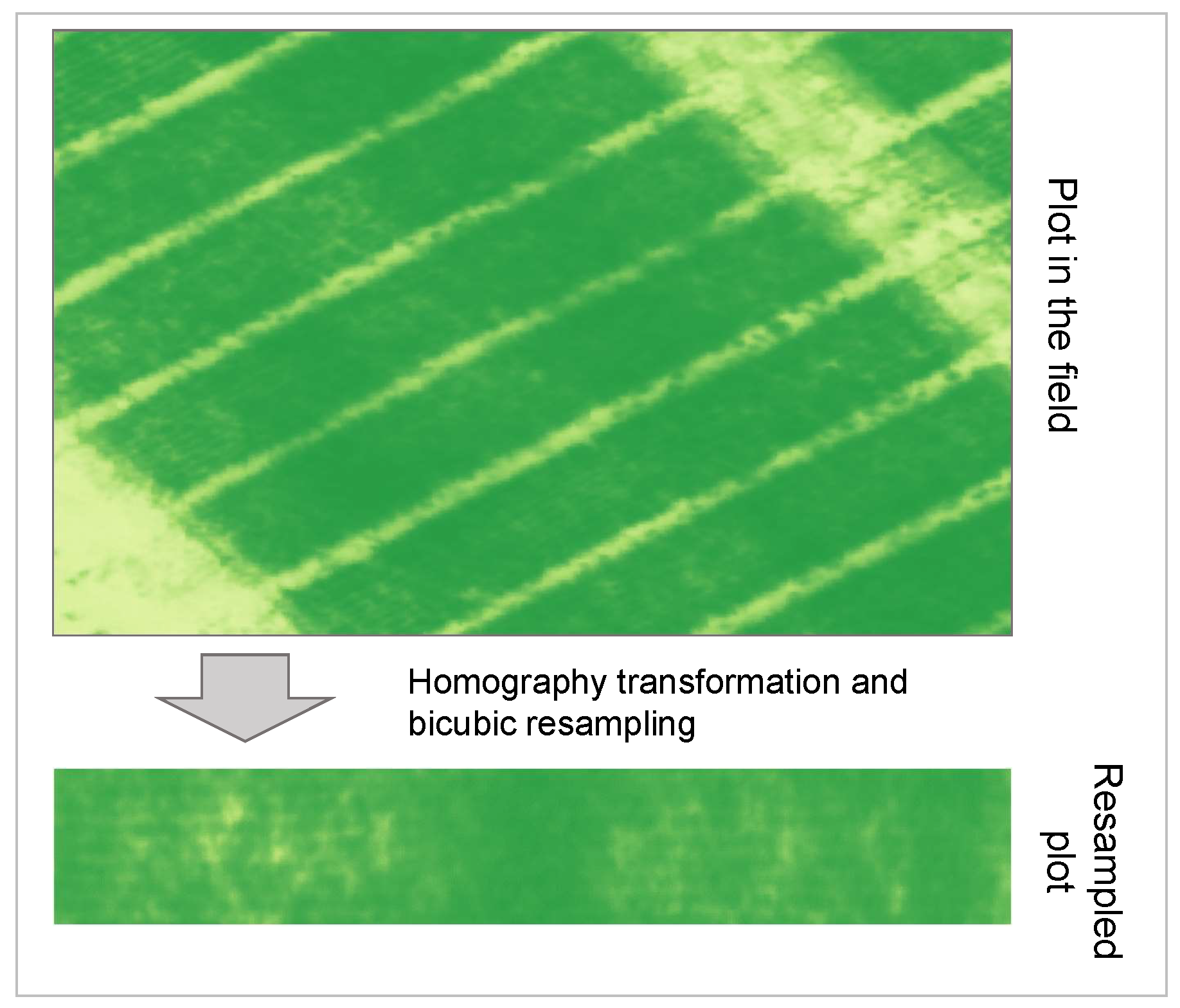
Figure 5.
Schematic representation of the TriNet network.
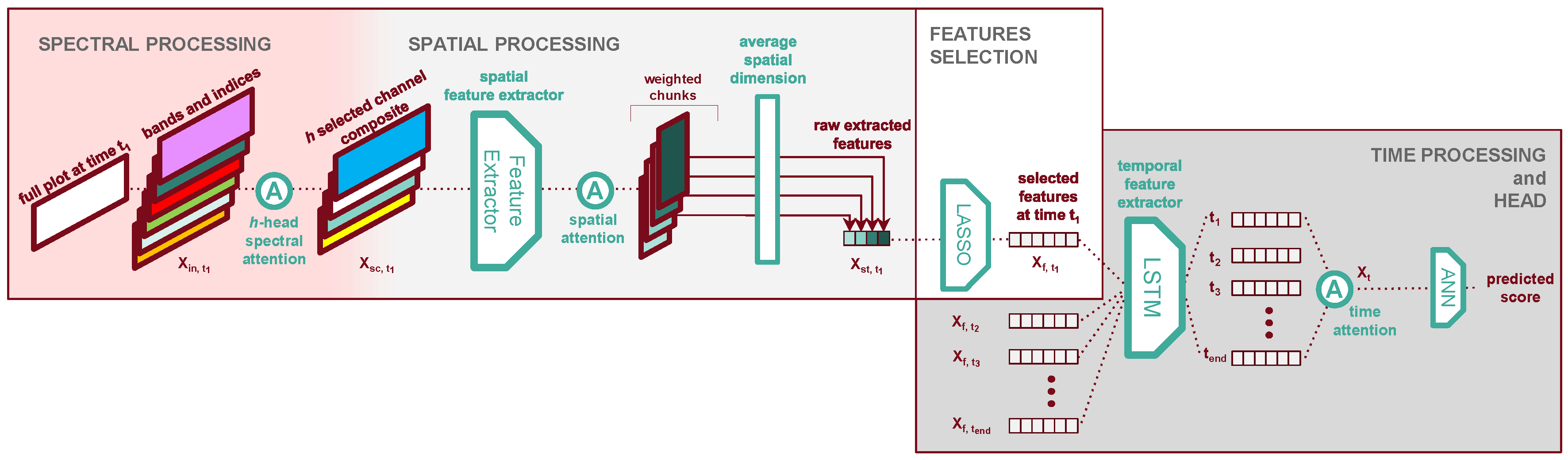
Figure 6.
Spatial processor module. The three components are in order: feature extraction, division in chunks, and attention between those chunks.
Figure 6.
Spatial processor module. The three components are in order: feature extraction, division in chunks, and attention between those chunks.
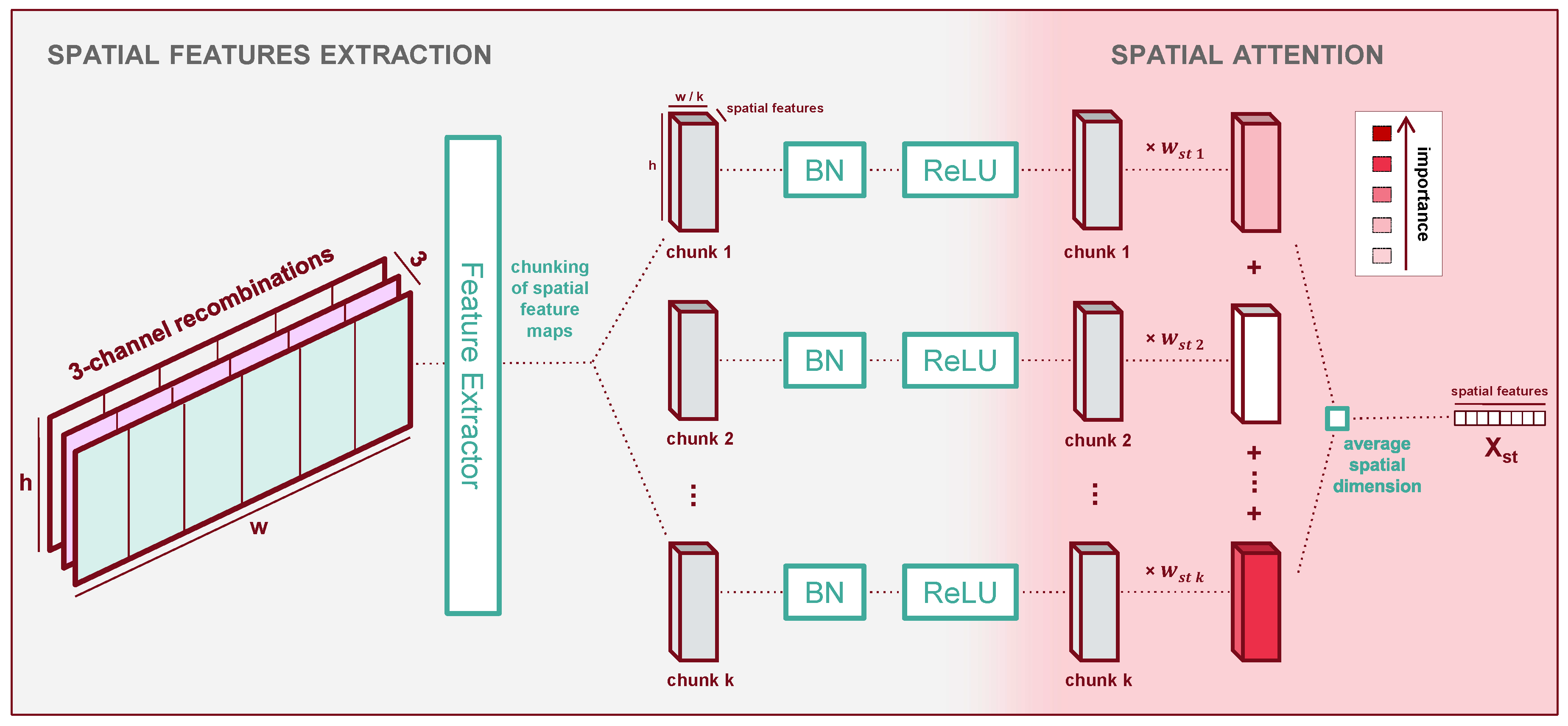
Table 1.
Synthesis of past studies on yellow rust prediction.
| Study | Key Findings | Accuracy | UAV | Target class # |
|---|---|---|---|---|
| [15] | Demonstrated the superiority of deep learning with a Multi-Layered Perceptron (MLP) achieving 99% accuracy in single leaf detection. | 99% | No | 2 classes |
| [16] | Utilised a Deep Convolutional Neural Network (DCNN) for wheat rust disease classification, achieving 97.16% accuracy in distinguishing healthy and diseased plants at the leaf level. | 97.16% | No | 2 classes |
| [17] | Processed phenocart-acquired data to predict yellow rust infection, revealing considerable infection and exploring the influence of different time steps on prediction. | 61% | No | 2 classes |
| [18] | Introduced a C-DenseNet architecture for wheat stripe rust disease grading, achieving a test accuracy of 97.99%. The dataset classifies leaf images with 6 levels of stripe rust infection. | 97.99% | No | 6 Classes |
| [19] | RustNet, based on ResNet-18, achieved accuracies between 79% and 86% on low-height flights. | 86% | Yes | 2 classes |
| [20] | Used hyperspectral data at 30 metres altitude to forecast yellow rust presence, achieving higher accuracy with Deep Convolutional Neural Network (DCNN) compared to basic methods. | 85% | Yes | 3 Classes |
| [21] | Explored a similar setup as in this study for spring wheat, emphasising the incorporation of temporal information in a 3D-CNN, achieving detection accuracy of 79% for spectral-spatio-temporal fused data. | 79% | Yes | 3 Classes |
Table 2.
Spectral Bands of Altum-PT Camera.
| Band | Center (nm) | Bandwidth (nm) |
|---|---|---|
| Blue | 475.0 | 32.0 |
| Green | 560.0 | 27.0 |
| Red | 668.0 | 16.0 |
| Panchromatic | 634.5 | 463.0 |
| Red edge | 717.0 | 12.0 |
| Near-IR | 842.0 | 57.0 |
| LWIR | 10.5 | 6.0 |
Table 3.
Vegetation Indices with Corresponding equations and sources.
| Index | Equation | Full Name | Source |
|---|---|---|---|
| Normalised Difference Vegetation Index | [36,37,38] | ||
| Soil Adjusted Vegetation Index | [39] | ||
| Optimised Soil Adjusted Vegetation Index | [40] | ||
| Enhanced Vegetation Index | [41] | ||
| Green Normalised Difference Vegetation Index | [42] | ||
| Green-Optimised Soil Adjusted Vegetation Index | [43] | ||
| Normalised Difference Red Edge | [44] | ||
| Canopy Chlorophyll Content Index | [45] | ||
| Green Chlorophyll Index | [46] | ||
| Pigment Specific Simple Ratio | [47,48] | ||
| Green Leaf Index | [46] | ||
| MCARI | Modified Chlorophyll Absorption in Reflectance Index | [49] | |
| RDVI | Renormalised difference vegetation index | [50] |
Table 7.
The Mean Square Error (MSE), the Mean Absolute Deviation (MAD), and some top-k accuracy results on all sets for our most explainable model, which we use to derive insights as explained in Section 3.4.
Table 7.
The Mean Square Error (MSE), the Mean Absolute Deviation (MAD), and some top-k accuracy results on all sets for our most explainable model, which we use to derive insights as explained in Section 3.4.
| Data split | MSE | MAD | Top-1 Accuracy | Top-2 Accuracy | Top-3 Accuracy |
| Train | 0.91 [0.72,1.15] | 0.74 [0.67,0.83] | 0.44 [0.38,0.51] | 0.77 [0.71,0.82] | 0.90 [0.86,0.94] |
| Validation | 1.45 [0.93,2.10] | 0.91 [0.74,1.10] | 0.38 [0.26,0.49] | 0.67 [0.57,0.78] | 0.84 [0.74,0.92] |
| Test 1 | 2.51 [0.99,4.81] | 1.23 [0.78,1.79] | 0.31 [0.08,0.60] | 0.52 [0.26,0.79] | 0.67 [0.40,0.89] |
| Test 2 | 2.69 [0.69,5.59] | 1.20 [0.68,1.91] | 0.35 [0.11,0.64] | 0.54 [0.27,0.81] | 0.70 [0.43,0.93] |
Table 8.
Results obtained with variants of the base model on the validation data. Line 1 is the base model presented in Table 5. Line 2 is the same architecture using only the best 3 selected bands and indices: EVI, red and GNDVI. Line 3 is the same architecture using only the Red, Green and Blue bands. Lines 4, 5 and 6 show the 5th, 50th and 95th percentiles of 30 independent models trained on random sets of three bands.
| Variant | Data split | MSE | MAD | Top-1 Accuracy | Top-2 Accuracy | Top-3 Accuracy |
| base model | Validation | 1.20[0.74,1.83] | 0.84[0.69,1.00] | 0.38[0.27,0.50] | 0.74[0.63,0.84] | 0.87[0.79,0.94] |
| EVI, red, GNDVI | Validation | 1.45 [0.91,2.05] | 0.91 [0.74,1.11] | 0.38 [0.27,0.50] | 0.67 [0.55,0.78] | 0.84 [0.75,0.92] |
| RGB only | Validation | 1.50 [0.94;2.38] | 0.92 [0.75;1.12] | 0.37 [0.26;0.48] | 0.68 [0.57;0.78] | 0.84 [0.75;0.92] |
| 5th percentile | Validation | 3.49 [1.54,6.63] | 1.50 [0.94,2.13] | 0.18 [0.01,0.41] | 0.37 [0.13,0.63] | 0.58 [0.33,0.84] |
| 50th percentile | Validation | 2.93 [1.17,5.62] | 1.33 [0.81,1.93] | 0.29 [0.07,0.55] | 0.45 [0.20,0.70] | 0.67 [0.40,0.88] |
| 95th percentile | Validation | 2.54 [0.92,4.81] | 1.23 [0.72,1.80] | 0.36 [0.12,0.63] | 0.52 [0.26,0.79] | 0.71 [0.47,0.93] |
Table 9.
Results obtained with variants of the base model on the validation data. Line 1 is the base model presented in Table 5. Line 2 is the same architecture using only the best 3 selected time steps: 5, 6 and 7. Lines 3, 4 and 5 show the 5th, 50th and 95th percentiles of 30 independent models trained on random sets of three time steps.
| Variant | Data split | MSE | MAD | Top-1 Accuracy | Top-2 Accuracy | Top-3 Accuracy |
| base model | Validation | 1.20[0.74,1.83] | 0.84[0.69,1.00] | 0.38[0.27,0.50] | 0.74[0.63,0.84] | 0.87[0.79,0.94] |
| Time steps 6 & 7 | Validation | 1.37 [0.89,2.00] | 0.90 [0.73,1.09] | 0.33 [0.22,0.44] | 0.66 [0.55,0.78] | 0.83 [0.74,0.91] |
| 5th percentile | Validation | 1.52 [1.24,1.84] | 4.05 [2.59,5.89] | 0.17 [0.09,0.27] | 0.36 [0.24,0.47] | 0.63 [0.51,0.74] |
| 50th percentile | Validation | 1.12 [0.92,1.36] | 2.21 [1.41,3.23] | 0.23 [0.13,0.33] | 0.58 [0.46,0.69] | 0.77 [0.67,0.86] |
| 95th percentile | Validation | 1.06 [0.83,1.26] | 1.89 [1.14,2.74] | 0.33 [0.23,0.45] | 0.63 [0.52,0.74] | 0.81 [0.72,0.89] |
Disclaimer/Publisher’s Note: The statements, opinions and data contained in all publications are solely those of the individual author(s) and contributor(s) and not of MDPI and/or the editor(s). MDPI and/or the editor(s) disclaim responsibility for any injury to people or property resulting from any ideas, methods, instructions or products referred to in the content. |
© 2024 by the authors. Licensee MDPI, Basel, Switzerland. This article is an open access article distributed under the terms and conditions of the Creative Commons Attribution (CC BY) license (http://creativecommons.org/licenses/by/4.0/).
Copyright: This open access article is published under a Creative Commons CC BY 4.0 license, which permit the free download, distribution, and reuse, provided that the author and preprint are cited in any reuse.


