Submitted:
19 August 2024
Posted:
20 August 2024
You are already at the latest version
Abstract
The advancements in social networking have empowered open expression on micro blogging platforms like Twitter. Traditional Twitter Sentiment Analysis (TSA) faced challenges due to rule-based or dictionary algorithms, dealing with feature selection, ambiguity, sparse data, and language variations. This study proposed a classification framework for Twitter sentiment data using word count vectorization and machine learning techniques to reduce the difficulties addressed on annotated sentiment-labelled tweets. Various classifiers (Naive Bayes, Decision Tree, K Nearest Neighbours, Logistic Regression, and Random Forest) were evaluated based on Accuracy, Precision, Recall, F1-score, and Specificity. Random Forest outperformed others with an Area under Curve (AUC) value of 0.96, and an Average Precision (AP) score of 0.96 in sentiment classification, especially effective with minimal Twitter-specific features.
Keywords:
Sentiment Classification
; Twitter Sentiment Analysis
; Word Count Vectorization
; Machine Learning
1. Introduction
In today’s digital landscape, user feedback, and reviews on social media platforms like Twitter, Facebook and Instagram hold significant value for organizations and play a predominant role aiming to enhance services, products and manage the whole performance efficiently. People can openly express their thoughts, ideas, and views as short messages called tweets on many micro blogging platforms in social networks and web forums [1]. Organizations frequently employ sentiment analysis or opinion mining techniques to extract meaningful information from the unstructured user inputs [2]. Sentiment analysis involves assessing emotions, opinions, and attitudes expressed within text data. Twitter serves as a rich source for the analysis due to its real-time nature and the vast amount of user generated content [3]. Notably, popular Twitter users like Justin Bieber receive over 300.000, an excessive volume of tweets every day. Similarly, accounts like Xbox Support, which have over 400,000 followers, face the daunting task of managing and responding to more than 1.5 million daily tweets. During notable events like the 2024 IPL match, Twitter experienced an even more significant surge, with over 750 million tweets related to the tournament sent during that time. Handling such massive datasets poses a considerable workload for any organization. The applications offered by TSA exhibit inadequate performance capabilities. According to a literature assessment, the accuracy metrics for sentiment analysis generally ranges from 40% to 80%. There is a need for more improved and precise TSA tools for firms in reviewing client feedback and analysing sentiments. Tweets use a wide-ranging, diverse, and ever-changing vocabulary that includes slang, acronyms, and emojis. Furthermore, tweets offer only a restricted number and shorter terms for sentiment analysis. This leads to tweet features having sparse representations, a common issue found with standard feature sets, which typically leads to the suboptimal performance of sentiment analysis algorithms.
Some of the key contributions in the article can be analysed from the following points:
- ▪
- Introduction of a Twitter-specific sophisticated Lexicon set to avoid ambiguity of sentiments in sentence level.
- ▪
- Analysis of Target class determination and Domain Adaptability using classifiers.
- ▪
- Implementation of MVT (Majority Voting Technique) with Random Forest classifier for improvement on Accuracy and other performance measures in sentiment analysis task.
The sequence of steps involved in the model have been depicted in Figure 1, that ultimately lead the classification of tweets as either Positive or Negative.
The subsequent sections of the article are structured as follows: Section 2 discusses related work, examining existing research in the domain. Section 3 introduces the proposed framework, providing an in-depth of its structure and components. Section 4 outlines vectorization techniques employed in the study. Section 5 illustrates various machine learning models. Section 6 furnishes dataset descriptions and wordcloud results. Section 7 is on Results and Discussion. Eventually ends with an outcome and future plans for more work.
2. Related Work
The primary objective of this study is to examine the application of Machine Learning techniques for sentiment classification. These techniques have been thoroughly reviewed and summarized by researchers and academics. The study concludes by providing different result approaches and machine learning algorithms tailored specifically for this research implementation. In sentiment analysis, the information has been reduced into a smaller subset referred to as the “sentiment lexicon”, which serves as a critical resource for sentiment algorithms. By leveraging the sophisticated lexicon set (SLS), the algorithms employed within the manuscript to retrieve access to a wide range of sentiments pertaining to emotions. This privilege facilitates to more accurately identify and separate the affective content expressed in the text with increased accuracy. Therefore, the principal aim of this work is to develop a concise, reliable, and reusable lexicon that can be utilized effectively to produce a better outcome for the model. The subsequent section highlights several contributions made by numerous researchers in the domain of related work on TSA.
F.M. Javed Mehedi Shamrat et al. [3] proposed a supervised KNN classification algorithm that extracts tweets from Twitter using API authentication token. The algorithm classifies the text in the dataset into three classes, positive, negative, and neutral. In [4] a novel architecture has been implemented for tweet sentiment classification exploiting the advantage of lexical dictionary and stacked ensemble of Long short-term memory (LSTM) as base classifiers and Logistic Regression (LR) as meta classifier. Mohit Dagar et al. [5] has applied two filters named as Sparse Feature Vector and Lexicon Feature Vector to identify the sentiments in the text is hatred or not hatered. The dataset has been analysed using weka software and the highest accuracy result they have achieved is with Random Forest technique. Stacked Weighted Ensemble (SWE) [6] proposed a sentiment detection model that integrates several independent classifiers like Hard voting, Soft voting, Linear Regression, Random Forest and Naïve Bayes. This model has utilized a variety of labelled grouping strategies to represent the order of emotions, including anger, fear, disgust, and cheer. Sentiment Specific Word Embedding (SSWE) [7] a technique addressed that learns vectorization for Twitter sentiment classification, which typically map words with similar syntactic context but opposite sentiment polarity such as good or bad.
Haowang Dogan Can et al. [8] proposed a sentiment analysis model and an annotation interface that allows the user to rate the sentiment toward the candidate's tweet mentioned as positive, negative or neutral or mark it as unsecure. There are also two options to specify whether a tweet is sarcastic and/or funny. Relief and gain information [9], are two approaches used for feature selection of spam profiles on Twitter. This study tested four classification methods and compared: multilayer perceptron, decision trees, naïve bayes and k-nearest neighbors. The advantage of this strategy is that it can achieve high detection rates regardless of the language used in tweets. The drawback of the technique is the poor accuracy rate due to the employment of small datasets for training. Arun Kumar Yadav et al. [10] proposed various machine learning and deep learning models for detection of hate speech utilizing various feature extraction and word embedding techniques on a consolidated dataset of 20600 instances with English-Hindi mixed tweets. S Saranya and G. Usha [11] implemented machine-learning based sentiment analysis method for feature extraction from Term Frequency and Inverse Document Frequency (TF-IDF), along with utilization of wordnet lemmatize and Random Forest (RF) network to detect sentiments from a Tweet. Study [12] Logistic Regression with Count Vectorizer (LRCV), a combined approach has been implemented by the authors on product reviews for sentiment analysis to convert text into numerical vectors, which further feed as input to the Machine Learning Model. The test has been conducted on benchmark datasets, producing better results across various performance metrics.
To conclude, from the extensive related work and literature survey, we observed significant contributions made by many researchers on TSA. The researchers have implemented different machine learning and deep learning algorithms on a wide range of datasets. However, the most significant research gap noticed is the absence of a proper dataset specifically tailored for TSA and an absence of comparisons among machine learning algorithms for sentiment analysis and classification.
In this regard, our proposed work makes a unique contribution for TSA in terms of the vectorization techniques, preprocessing steps used, algorithms implemented for sentiment classification, and finally the utilization of statistical and analytical approaches to interpret the results. To address and understand Twitter Sentiment Analysis, various research questions are addressed as follows:
2.1. Research Questions and Inferences in TSA
In context with TSA, research questions and inferences focus on understanding the sentiment (positive, negative) expressed in tweets.
Here are some research questions and potential conclusions related to TSA.
RQ1: What factors influence Twitter sentiment polarization during public events?
A variety of factors can influence Twitter sentiment polarization during public events. These factors can contribute to the division of opinions, resulting to a strong separation between positive and negative sentiments. The list includes event controversy, political or ideological affiliations, media coverage and framing, inflammatory tone and language, misinformation etc.
RQ2: What factors of Twitter has been chosen as the target platform for the study of Sentiment Analysis?
Twitter has been chosen as a popular platform because of its increasing number of active users every time span, and the platform can make it brief and simple to collect vast quantities of passionate and real time text data. Furthermore, it often includes hash tags and keywords to categorize and highlight the tweets which give researchers insights, allowing a deeper understanding of sentiment dynamics.
RQ3: Can sentiment analysis on Twitter provide more timely and accurate insights compared to traditional methods?
TSA can provide more timely insights than traditional methods of tracking public opinion, thus allowing for a quicker identification of emerging trends and events, on the other hand, traditional methods like surveys might take more time to design, conduct and analyze which could lead to delay in capturing the current sentiment.
RQ4: Could sentiment analysis benefit from integrating visual content (images and videos) alongside textual analysis within tweets?
Yes, combining textual analysis of tweets with visual content could be helpful for sentiment analysis. The accuracy and depth of sentiment analysis results can be improved by using visual content, which can give context and clues that may not be available in the text alone.
3. Proposed Framework
The main emphasis and objective of this study are to analyze the sentiments and opinions expressed in tweets. Our work aims to create precise and robust machine learning techniques employing vectorization methods and classifiers. In order to optimize the data for machine processing vectorization techniques such as CBow and skip-gram are used to transform the cleaned and refined data into formats that are numerical in nature. The analysis is segmented into distinct phases as highlighted in Figure 2. The initial phase encompasses data collection from the Twitter database and API. Following this, the selection of a suitable dataset and the subsequent phases involve the preprocessing of data, vector representation, term frequency calculation, sentiment analysis, execution of different classifiers, and ultimately choosing the most optimal classifier that produces the finest outcome for sentiment classification, effectively categorizing as positive or negative. The steps of data preprocessing have been summarized.
3.1. Data Preprocessing
A crucial data mining approach is to preprocess real-world data into a more comprehensive and consistent format. Before beginning any analysis, it is critical to address the inconsistency and missing aspect of Twitter data. Many rounds of preprocessing steps are performed on the tweets before they are ready for further analysis.
3.2. Text Cleaning and Tokenization
The initial stage of this process involves the elimination of special characters, URLs, hash tags, stop words, mentions, emojis, and HTML tags. Subsequently, the text has been split into discrete words or tokens. Its application ensures that the text is ready for a wide array of natural language processing applications, leading to more meaningful and accurate findings.
3.3. Lemmatization
The texts are lemmatized after stop words are eliminated. Examples include changing the words “running” to “run”. As a result, any instances of non-English words are removed during preprocessing. The subsequent phase involves the n-gram construction, which is a crucial step in text analysis tasks like sentiment classification, especially for platforms like Twitter with concise and casual texts.
3.4. N-gram Construction
N-grams are contiguous occurrences of n items, In essence constructing n-grams serves to capture nearby contextual information that carries significance for the study. Following this phase, the word count vectorization technique is employed.
3.5. Vector Representation
This technique is used to transform collection of raw textual data into vectors of continuous real numbers. The occurrence of specific terms or phrases is assessed through frequency analysis. Subsequently an AI classifier is integrated into the pipeline, accurately classifies the sentiment of each tweets using machine learning algorithms. A thorough evaluation evaluates accuracy and other performance criteria to determine the most optimal classifier. Pseudocode 1, outlines the detailed steps of the proposed framework.
Pseudocode1 of proposed framework
----------------------------------------------------------------------------------------------------------------
1: Input dataset (ds) with corresponding sentiment labels (positive, negative)
2: for each sample in the ds do
3: Pre-process the input text (sample.text (Text cleaning and Tokenization, Lowercasing, Lemmatization, n- gram construction))
4: Feature extraction creating a vocabulary from the tokenized tweets and representing each tweet as a vector of word frequencies in the vocabulary.
5: Vector representation using (CBoW, Skip-gram) converting each tweet into a numerical value.
6: Implement the sentiment classification algorithm (NB, DT, KNN, LR, RF)
7: Split pre-processed (ds) into training and testing sets.
8: for each model in models do
9: TrainModel= (model, ds, tr (training_data))
10: Performance_metrics (pt) = (model, ds, td (testing_data))
11: CapturePerformanceMetrics (model, pt)
12: end for:
13: Optimal_classifier =SelectOptimalClassifier (model, pt)
14: End.
----------------------------------------------------------------------------------------------------------------
4. Vectorization Approach for Machine Learning Techniques
Word embedding is a method that transforms individual terms into a distinct vector representation, considering both their syntactic and semantic contexts. This approach enables to determine how similar a term is in relation to others in a tweet. Words are represented by vectors that are trained using neural networks to fit within a predefined vector space. The learning procedure can be executed through either a supervised neural network model or an unsupervised approach that leverages document statistics. Figure 3. illustrates different words embedding techniques which can be used depending on the context and type of applications.
Word Embedding can be classified into two main types: Frequency Based and Prediction Based embeddings. Representing words numerically present several challenges. One such technique, the Bag of Words, although it produces acceptable outcomes, but lacks of ordering preservance, assigns values of either 0 or 1, making incapable to derive the most significant words. To address this limitation, we can turn into another technique called TF-IDF. Some of the word embedding techniques outlined in Figure 2. has been explained to improve readability.
4.1. TF-IDF
This simple and straightforward technique assigns weight to words based on their occurrence and importance in a document, making it easy to understand which words contribute to sentiment. However, this technique has limitations in capturing context, semantics, and word order, which are important aspects of sentiment analysis on social media data.
Below is the equation to calculate TF-IDF.
For the word i in document j, f (i, j) represents the frequency of the term i in document j. This basically indicates the number of times term i appears in document j.f (i) represents the overall number of occurrences of term i in the entire collection of documents. N represents the aggregate number of documents in the collection.
4.2. Co-Occurrence Matrix
This is an effective technique for capturing semantic information from the text, but they have drawbacks related to high dimensionality, sparsity, word loss, and memory requirements. In response to the limitations of frequency-based word embeddings, this study explores a more sophisticated approach employing, prediction-based word embedding techniques such as Word2Vec.
4.3. Word2Vec
It is a two-layer neural network model that has been applied to produce word embeddings within a vector space and identify patterns in word association in a large text corpus [10]. It preserves the relationship between words encompassing synonyms and antonyms, thereby facilitating a contextual understanding that proves valuable for identifying sentiment relevant words and their polarities. Additionally, Word2Vec employs two algorithms for the task of generating vectors from words: CBow (Continuous Bag of words) and Skip-gram.
4.4. CBow
This is a most popular word embedding technique which predicts the actual target word from the context words. Figure 4. depicts the working principle of the technique with an example. Here a Tweet sentence is taken. To predict the target word (“Excitement”), it has taken two context words (“is” and “building”). The words are initially converted into one hot encoding vector representations (One hot vector-one bit is “1”, all other bits are “0” and vector length= No of words in sentence) which is shown in the Figure. Next step is to select the window size to iterate over the sentence. The window size is-3 and the neural network is taken which has the context words as input share the 5x3 matrix and we pass the one hot vector of “is” and “building” to the neural network that tries to predict the target word.
4.5. Skip-Gram
The NLP technique, employed in this study, serves as a counterpart to CBow used for word embedding, a technique of representing words as condensed vectors within a continuous vector space. This approach is used to learn word embeddings by forecasting the context words based on the target word. It possesses the capability to capture semantic relationships between words, as words have analogous meanings tends to have similar embeddings. Figure 5. visually illustrates the operational principles of this renowned technique.
5. Machine Learning Models
In this study, five distinct classifiers have been implemented with word embedding techniques that leverage a variety of classification techniques. Sentiment classification on Twitter involves the apply of Machine Learning models to automatically examine and classify the sentiment or emotion conveyed within tweets. The next subsections discuss various approaches and the classifiers employed within the scope of this study.
5.1. Naïve Bayes (NB)
The NB model is a popular probabilistic categorization method based on Baye’s theory. It attempts to establish the probability associated with a specific set of attributes. The NB technique proves valuable when classifying feature sets that exhibit interdependencies among their features. The NB classifier is based on Bayes’ theorem, which determines the likelihood of a specific sentiment class (positive, negative) given the words in the tweet. The classifier estimates the probability distribution of words in each sentiment class during training [12].
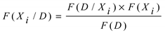
The Bayes' theorem is used in this work to calculate the operational probability of the Naïve Bayes classifier for a given dataset D with classes Xi.
5.2. Decision Tree (DT)
The decision tree technique, which is commonly used in traditional learning theory, evaluates the informational relevance of a given dataset by utilizing the renowned Shannon's entropy model [14]. We applied the C4.5 approach to create decision rules for our classification system, a version of the decision tree methodology, within the scope of this study. We created a decision tree using the C4.5 method that systematically divides the data consistently according to the information gathered from Shannon's entropy model. By using this method, the model can successfully recognize the significant features and create protocols that enable the correct feature classification within the dataset. The DT is a valuable algorithm for managing and evaluating complicated data structures, facilitating for intelligent choices in decision-making across several fields.
5.3. K-Nearest Neighbor (K-NN)
K-Nearest Neighbour (K-NN) classifiers are essential for determining the class of an unknown instance. This algorithm finds the length of uninterrupted distance between two objects, denoted as x and y, where x stands for known data points and x∈X, where X is a predetermined dataset. The objective is to find the class of instance y for which the class must be defined. To increase the forecast precision of this approach, it is possible to apply a weight function, represented as, in distance computations. This weight function adds the ability to assign different amounts of priority to different distances, which impacts the outcomes of predictions. The K- NN method finds the correlation between examples using a distance measurement, allowing for trustworthy categorization. The distance function of the K-NN algorithm has the following mathematical expression.
5.4. Logistic Regression (LR)
The logistic function operates as the algorithm’s vital operation has been taken into account. This technique principally dependent on the sigmoid function. It generates curve of S-shaped that accurately alters the input domain’s real values to a narrower range from 0 and 1. The application can accurately process and interpret static numerical input to this mathematical adjustment. The word "logistic" is originated from the basic characteristics of the sigmoid function, enhancing the algorithm to model and explore detailed as well as complex relationships in the data. We can define the sigmoid function as follows:
Here:
- σ(x) represents the sigmoid function.
- e is the base of the natural logarithm, close to 2.71828.
- x is the function’s input value.
5.5. Random Forest (RF)
The Random Forest classifier utilizes and integrates number of decision trees randomly to speed up classification for the Twitter sentiment dataset over the input vector. It examines the collective prediction output from these decision trees using the Majority Voting Technique (MVT). The coupled decision trees may now forecast future events by selecting the most prevalent class. As a result, these characteristics strengthen the RF classifier's robustness in resolving real-world challenges and highlight its effectiveness in handling multi-class datasets.
Employing MVT, it becomes evident that the Random Forest (RF) a binary classifier outperforms all other classifiers in achieving optimal result. Figure 6. Visually illustrates the operational framework of this classifier, employing a specific number of Decision Trees as Base Learners. The classifier incorporates Row Sampling and Feature Sampling technique with input data supplied to the model for output verification. In this context, when employing maximum no of base learners, the resulting output is 0. Consequently, through the application of Majority Voting Technique, the resulting output is determined to be 0. This RF classifier effectively removes over fitting issues and attains highest accuracy in sentiment classification.
6. Dataset Description
Studies that perform sentiment classification either generate their own data or utilize pre-existing datasets. Creating a new dataset enables the use of statistical information and data pertinent to the problem being addressed by the analysis. However, labeling the dataset, which can be rather hard, presents a considerable challenge. Furthermore, producing a significant volume of data is not always an easy undertaking. Thus, we have chosen the datasets for our work, which is widely accepted by the research community.
The details of these datasets are outlined below:
- Twitter_hatespeech dataset is used in this study comprising 48813 tweets already labeled with sentiment polarity conveyed (0=negative, 1=positive).
- Additionally, the Twitter_ parsed dataset containing 21907 tweets with the same polarity labels (0=negative, 1=positive) was used as a second dataset.
- The two datasets were merged based on their features, resulting in a combined dataset of 70720 tweets. These tweets were categorized into positive and negative classes for further analysis.
- Figure 7. Provides a clear and perceptive understanding of the distribution of Positive and Negative tweets in our dataset.
Figure 8 displays an original sample of tweets in the dataset and after Pre-processing. It contains information on each of the following fields:
- “index” is the sample no.
- “id” is the unique id of each tweet.
- “label” is the polarity of the tweet.
- “tweet” is the tweets exact wording.
6.1. Wordcloud
Wordcloud is used in this study to access visual representation of text data, where words are displayed in varying sizes and colors based on their frequency and importance within the scope. This powerful tool is leverage to extract the most prominent positive and negative tweets from the dataset employed. Figure 9. illustrates the visualizations of these findings.
7. Results and Discussion
The dataset contains 70720 tweets, split into training and testing sets following the 70-30 rule, with 70% of data allocated for training and the remaining 30% for testing. To assess the effectiveness of our chosen methodologies, we employed a set of performance metrics, including Accuracy, Precision, Recall, F1-score, Specificity (Negative Recall), and ROC_AUC. Below are the equations for the discussed performance metrics.
The accuracy measure provides how many data points are correctly predicted.
The Precision measure calculates the number of actually positive samples among all the predicted positive class samples.
Recall (or Sensitivity) calculates how many test case samples are predicted correctly among all the positive classes.
F1-Score is the harmonic mean of Precision and Recall.
Negative Recall (or Specificity) computes how many test case samples are predicted correctly among all the negative classes.

Table 1.
Performance Measures (in percentage) for sentiment classification.
| Performance Measures | NB | DT | KNN | LR | RF |
| Accuracy | 81.77 | 4.55 | 89.43 | 87.44 | 96.10 |
| Precision | 87.75 | 97.94 | 91.80 | 86.98 | 98.91 |
| Recall | 73.82 | 90.06 | 86.57 | 88.02 | 93.34 |
| F1-Score | 80.19 | 94.29 | 89.11 | 87.50 | 96.01 |
| Specificity | 73.81 | 90.04 | 86.56 | 88.01 | 92.91 |
| ROC_AUC | 81.77 | 94.55 | 89.43 | 87.44 | 96.15 |
7.1. Comparative Analysis through Evaluation Metrics
In our comprehensive evaluation depicted in Figure 10(a), notably, Random Forest (RF) achieved an impressive accuracy %, surpassing of 96.15the accuracy of NB (81.77%), DT (94.55%), KNN (89.43%), and LR (87.44%).
Furthermore, RF emerged as the most precise classifier with precision of 98.91% compared to NB (87.55%), DT (97.94%), KNN (91.8%), and LR (86.98%), as highlighted in Figure 10(b). Additionally, RF exhibited a remarkable recall rate of 93.34%, exceeding NB (73.82%), DT (90.06%), KNN (86.57%), and LR (88.02%) as illustrated in Figure 10(c). In terms of F1-score, RF excelled with a rate of 96.01%, eclipsing NB (80.19%), DT (94.29%), KNN (89.11%), and LR (87.5%), as shown in Figure 10(d). Moreover, RF displayed a specificity rate of 92.91% in Figure 10(e), outperforming NB (73.81), DT (90.04%), KNN (85.56%), and LR (88.01%). Finally, RF demonstrated superior predictive performance achieving an ROC_AUC rate of 96.15% as illustrated in Figure 10(f). This performance clearly outpaced NB (81.77%), DT (94.55%), K-NN (89.43%), and LR (87.44%). These findings emphasize RF’s exceptional performance and reliability across a range of evaluation metrics.
7.2. Analysis through Confusion Matrix
Confusion Matrix is a performance evaluation tool for classification models, breaking down predictions into categories of TP (True positives), TN (True Negatives), FP (False positives), and FN (False Negatives). In Figure 11(a), the confusion matrix for NB classifier is illustrated. The matrix includes the values as TP-8349, FP-1165, FN-2960, and TN-10162.Furthermore the confusion matrix for DT classifier is highlighted in Figure 11(b), and the values are as TP-11218, FP-1123, FN-109, and TN-10186.
Moreover, in Figure 11(c), the matrix reveals the values as TP-9791, FP-874, FN-1518, and TN-10453 for KNN classifier. Additionally in Figure 11(d), the matrix for LR classifier is presented with specific values as TP-9955, FP-1439, FN-1354, and TN-9838. Finally, Figure 11(e), the emerged RF classifier outlines the values for the confusion matrix as TP-10556, FP-116, FN-753, and TN-11211.
This indicates that the Random Forest (RF) classifier exhibits a remarkable True Positive rate while maintaining an extremely Low False positive rate. Above is the illustration of the Confusion Matrix for NB, DT, KNN, LR, and RF classifiers.
The effectiveness and performance of the classifier upgrades as the graph approaches the top-left corner one popular analytics for compressing a classifier’s overall performance is the area under the ROC curve (ROC-AUC). Its values vary from 0 to 1, with 1 denoting perfect classification and 0.5 denoting inconsistent grouping. The research shows that out of the five algorithms used, for sentiment analysis on Twitter data, the RF classifier exhibits the optimal convergence. The average precision score it receives is 0.96, meaning that it effectively identifies almost all positive cases and thus producing less false positives.
The ROC curves for NB, DT, KNN, LR, and RF classifiers were displayed in Figure 12(a). This was observed that the RF classifier presents superior AUC value, which was as high as 0.96. This demonstrates that the RF classifier detects positive sentiment from Twitter data with an excellent degree of precision. Furthermore, due to the curve’s close placement to the top-left corner, the ROC-AUC shows great performance.
Figure 12(b), highlights the precision recall curves for NB, DT, KNN, LR, and RF classifiers along with the average precision score. It is noticed that the highest AP score was viewed for RF classifier with AP score=0.96.ROC curve displays how, as the classification threshold changes, the relationship between the true positive rate (sensitivity) and the false positive rate (specificity - 1) adjusted.
7.3. Comparison study
In this work, we closely examine and compare several sentiment classification algorithms used on Twitter data as illustrated in Table 2. Due to the informal language, shortness, and diverse expression [22] used by the users, sentiment analysis on social media sites, particularly Twitter presents unique challenges. To address these challenges, we explore the effectiveness of several machine learning algorithms. Also, as sentiment analysis is being utilized in various corporate sectors for review of products, it is equally important to check whether the text posted is positive, negative or neutral [23].
8. Conclusions and Future Work
This research contributes empirical insights to the fields of sentiment analysis and data science. It involves a comparison of various conventional categorization techniques to assess their accuracy. Notably, there is a scarcity of studies focused on sentiment analysis using Twitter data. Prior research predominantly examined tweets at the word level, disregarding word order. However, this study employs document vectors (Word2vec) to analyze tweets at the phrase level, taking word order into account. By incorporating the RF algorithm, a robust classifier was developed, yielding an AUC value of 0.96 and an average precision score of 0.96.
The high accuracy levels of these classifiers hold promise for investigating user satisfaction within the realm of sentiment analysis. However, the primary limitation lies in the relatively small sample size used to train the model, indicating potential for further enhancement. Strengthening the model and improving categorization accuracy can be achieved by augmenting the number of tweets utilized in the analysis.
References
- Poomka, Pumrapee, Nittaya Kerdprasop, and Kittisak Kerdprasop. "Machine learning versus deep learning performances on the sentiment analysis of product reviews." International Journal of Machine Learning and Computing 11, no. 2 (2021): 103-109. [CrossRef]
- Umarani, V., Anitha Julian, and J. Deepa. "Sentiment analysis using various machine learning and deep learning Techniques." Journal of the Nigerian Society of Physical Sciences (2021): 385-394. [CrossRef]
- Shamrat, F. M. J. M., Sovon Chakraborty, M. M. Imran, Jannatun Naeem Muna, Md Masum Billah, Protiva Das, and O. M. Rahman. "Sentiment analysis on twitter tweets about COVID-19 vaccines using NLP and supervised KNN classification algorithm." Indonesian Journal of Electrical Engineering and Computer Science 23, no. 1 (2021): 463-470. [CrossRef]
- Gaye, Babacar, Dezheng Zhang, and Aziguli Wulamu. "A tweet sentiment classification approach using a hybrid stacked ensemble technique." Information 12, no. 9 (2021): 374. [CrossRef]
- Dagar, Mohit, Abhishek Kajal, and Pardeep Bhatia. "Twitter sentiment analysis using supervised machine learning techniques." In 2021 5th International Conference on Information Systems and Computer Networks (ISCON), pp. 1-7. IEEE, 2021.
- Kokatnoor, Sujatha Arun, and Balachandran Krishnan. "Twitter hate speech detection using stacked weighted ensemble (SWE) model." In 2020 Fifth International Conference on Research in Computational Intelligence and Communication Networks (ICRCICN), pp. 87-92. IEEE, 2020.
- Tang, Duyu, Furu Wei, Nan Yang, Ming Zhou, Ting Liu, and Bing Qin. "Learning sentiment-specific word embedding for twitter sentiment classification." In Proceedings of the 52nd Annual Meeting of the Association for Computational Linguistics (Volume 1: Long Papers), pp. 1555-1565. 2014.
- Wang, Hao, Doğan Can, Abe Kazemzadeh, François Bar, and Shrikanth Narayanan. "A system for real-time twitter sentiment analysis of 2012 us presidential election cycle." In Proceedings of the ACL 2012 system demonstrations, pp. 115-120. 2012.
- Ala'M, Al-Zoubi, Ja'far Alqatawna, and Hossam Paris. "Spam profile detection in social networks based on public features." In 2017 8th International Conference on information and Communication Systems (ICICS), pp. 130-135. IEEE, 2017.
- Patel, Ravikumar, and Kalpdrum Passi. "Sentiment analysis on twitter data of world cup soccer tournament using machine learning." IoT 1, no. 2 (2020): 14. [CrossRef]
- Saranya, S., and G. Usha. "A Machine Learning-Based Technique with IntelligentWordNet Lemmatize for Twitter Sentiment Analysis." Intelligent Automation & Soft Computing 36, no. 1 (2023). [CrossRef]
- Jayakody, J. P. U. S. D., and B. T. G. S. Kumara. "Sentiment analysis on product reviews on twitter using Machine Learning Approaches." In 2021 International Conference on Decision Aid Sciences and Application (DASA), pp. 1056-1061. IEEE, 2021.
- Rodrigues, Anisha P., Roshan Fernandes, Adarsh Shetty, Atul K, Kuruva Lakshmanna, and R. Mahammad Shafi. "[Retracted] Real-Time Twitter Spam Detection and Sentiment Analysis using Machine Learning and Deep Learning Techniques." Computational Intelligence and Neuroscience 2022, no. 1 (2022): 5211949.
- Ala'M, Al-Zoubi, Ja'far Alqatawna, and Hossam Paris. "Spam profile detection in social networks based on public features." In 2017 8th International Conference on information and Communication Systems (ICICS), pp. 130-135. IEEE, 2017.
- Patel, Ravikumar, and Kalpdrum Passi. "Sentiment analysis on twitter data of world cup soccer tournament using machine learning." IoT 1, no. 2 (2020): 14. [CrossRef]
- Shafin, Minhajul Abedin, Md Mehedi Hasan, Md Rejaul Alam, Mosaddek Ali Mithu, Arafat Ulllah Nur, and Md Omar Faruk. "Product review sentiment analysis by using nlp and machine learning in bangla language." In 2020 23rd International Conference on Computer and Information Technology (ICCIT), pp. 1-5. IEEE, 2020.
- Zhang, Lei, Riddhiman Ghosh, Mohamed Dekhil, Meichun Hsu, and Bing Liu. "Combining lexicon-based and learning-based methods for Twitter sentiment analysis." HP Laboratories, Technical Report HPL-2011 89 (2011): 1-8.
- Basari, Abd Samad Hasan, Burairah Hussin, I. Gede Pramudya Ananta, and Junta Zeniarja. "Opinion mining of movie review using hybrid method of support vector machine and particle swarm optimization." Procedia Engineering 53 (2013): 453-462. [CrossRef]
- Bohra, Aditya, Deepanshu Vijay, Vinay Singh, Syed Sarfaraz Akhtar, and Manish Shrivastava. "A dataset of Hindi-English code-mixed social media text for hate speech detection." In Proceedings of the second workshop on computational modeling of people’s opinions, personality, and emotions in social media, pp. 36-41. 2018.
- Dang, Nhan Cach, María N. Moreno-García, and Fernando De la Prieta. "Sentiment analysis based on deep learning: A comparative study." Electronics 9, no. 3 (2020): 483. [CrossRef]
- Musleh, Dhiaa A., Ibrahim Alkhwaja, Ali Alkhwaja, Mohammed Alghamdi, Hussam Abahussain, Faisal Alfawaz, Nasro Min-Allah, and Mamoun Masoud Abdulqader. "Arabic sentiment analysis of youtube comments: Nlp-based machine learning approaches for content evaluation." Big Data and Cognitive Computing 7, no. 3 (2023): 127. [CrossRef]
- Kastrati, Zenun, Fisnik Dalipi, Ali Shariq Imran, Krenare Pireva Nuci, and Mudasir Ahmad Wani. "Sentiment analysis of students’ feedback with NLP and deep learning: A systematic mapping study." Applied Sciences 11, no. 9 (2021): 3986. [CrossRef]
- Mitra, Ayushi, and Sanjukta Mohanty. "Sentiment analysis using machine learning approaches." Emerging Technologies in Data Mining and Information Security: Proceedings of IEMIS 2 (2020): 63-68.
Figure 1.
Machine Learning Pipeline for Sentiment Analysis.
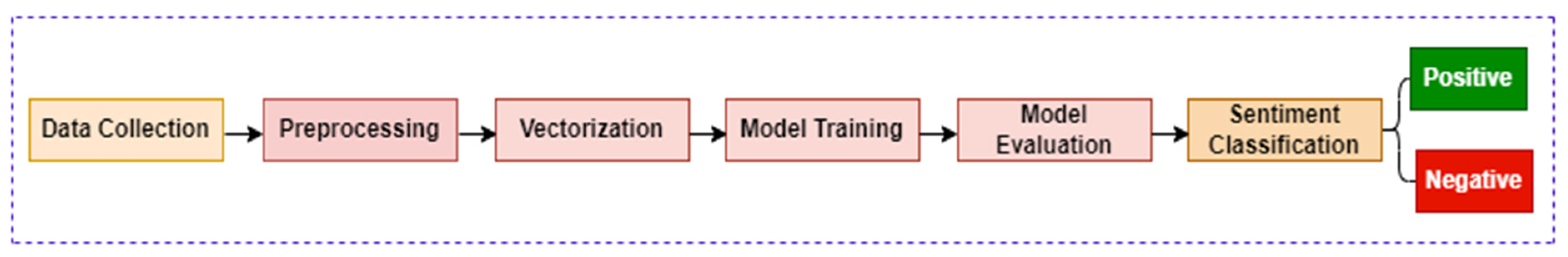
Figure 2.
Proposed Twitter Sentiment Classification Approach.
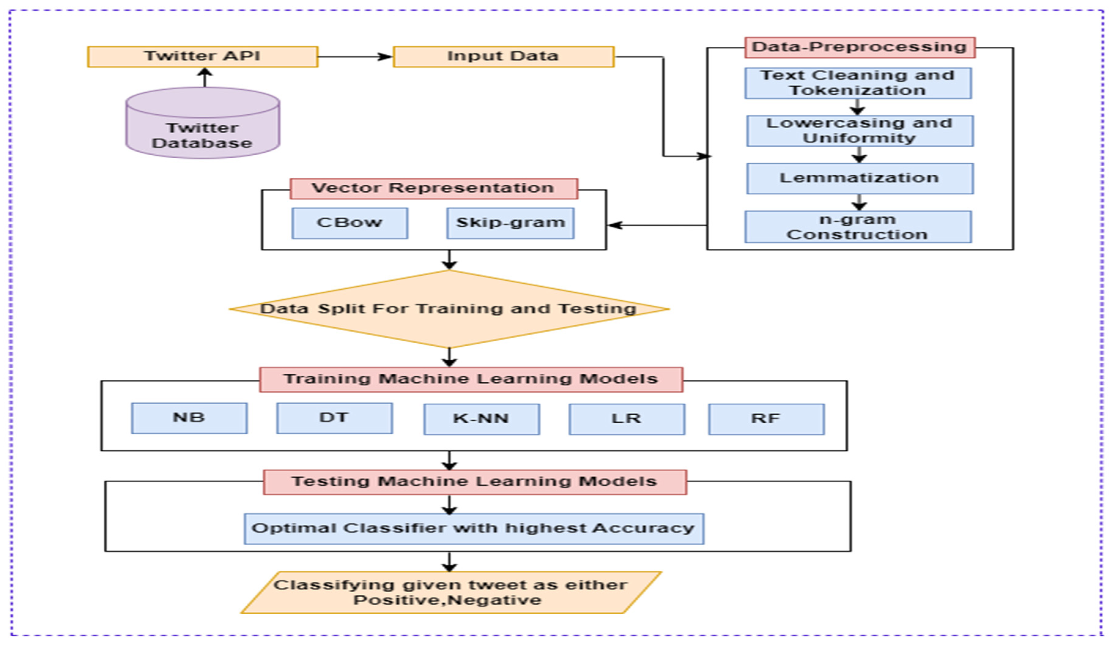
Figure 3.
Word Embedding Techniques.
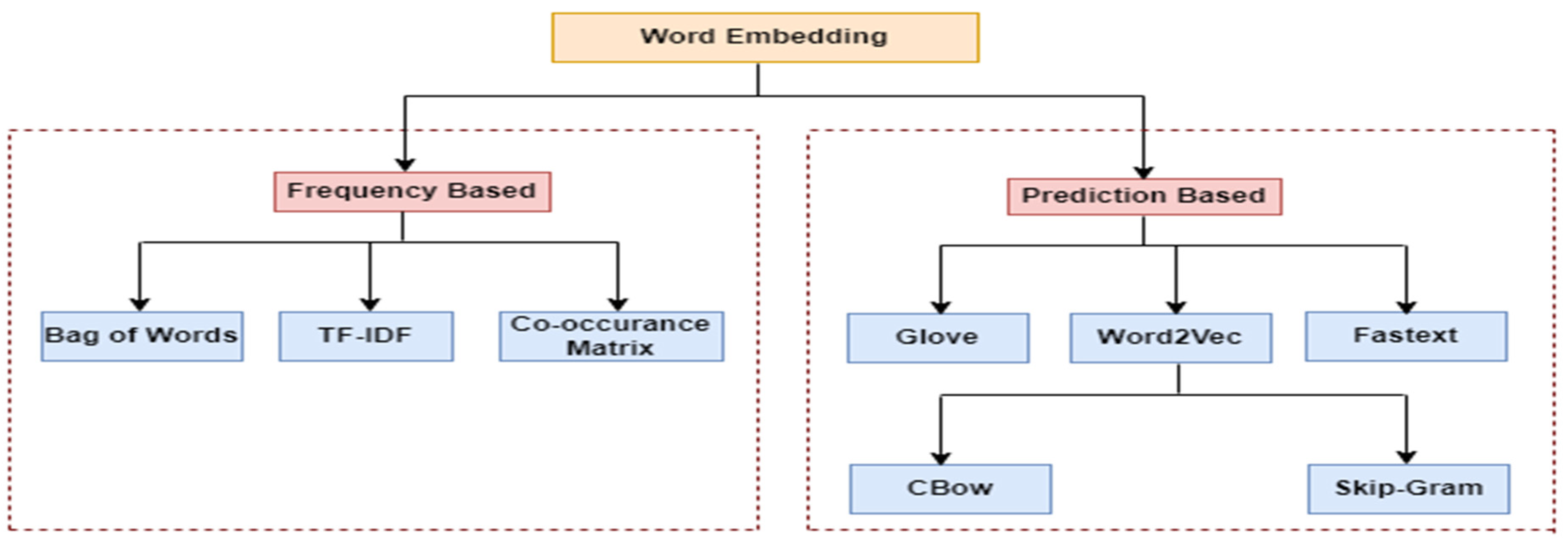
Figure 4.
Working Principle of CBow Technique.
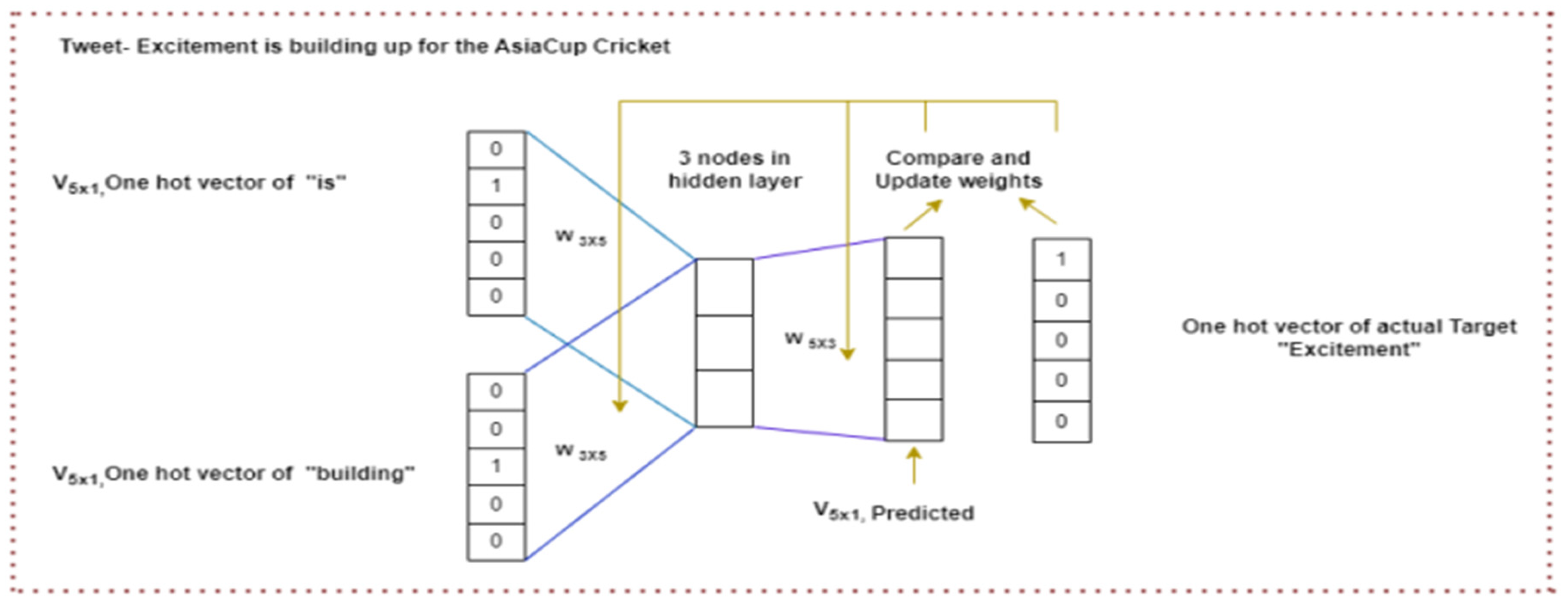
Figure 5.
Working Principle of Skip-Gram Technique.
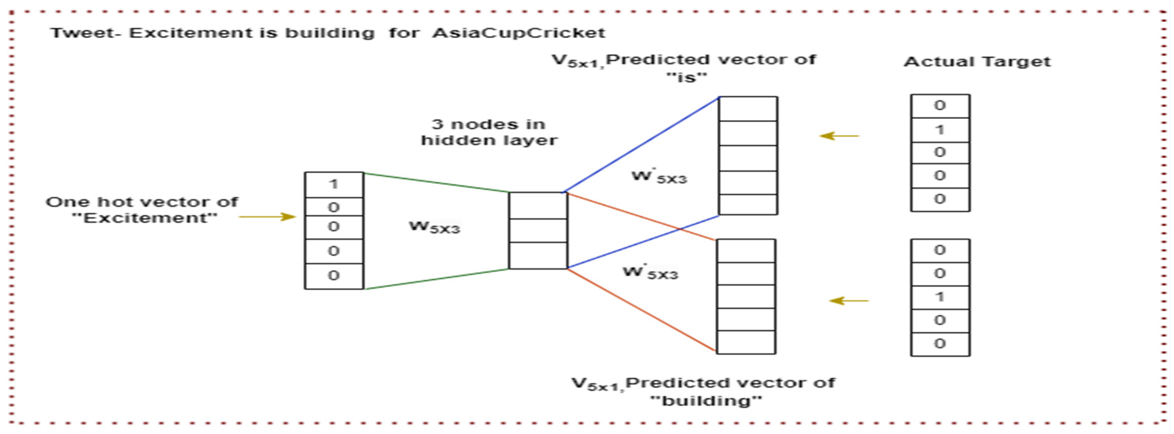
Figure 6.
Random Forest using Majority Voting Technique.
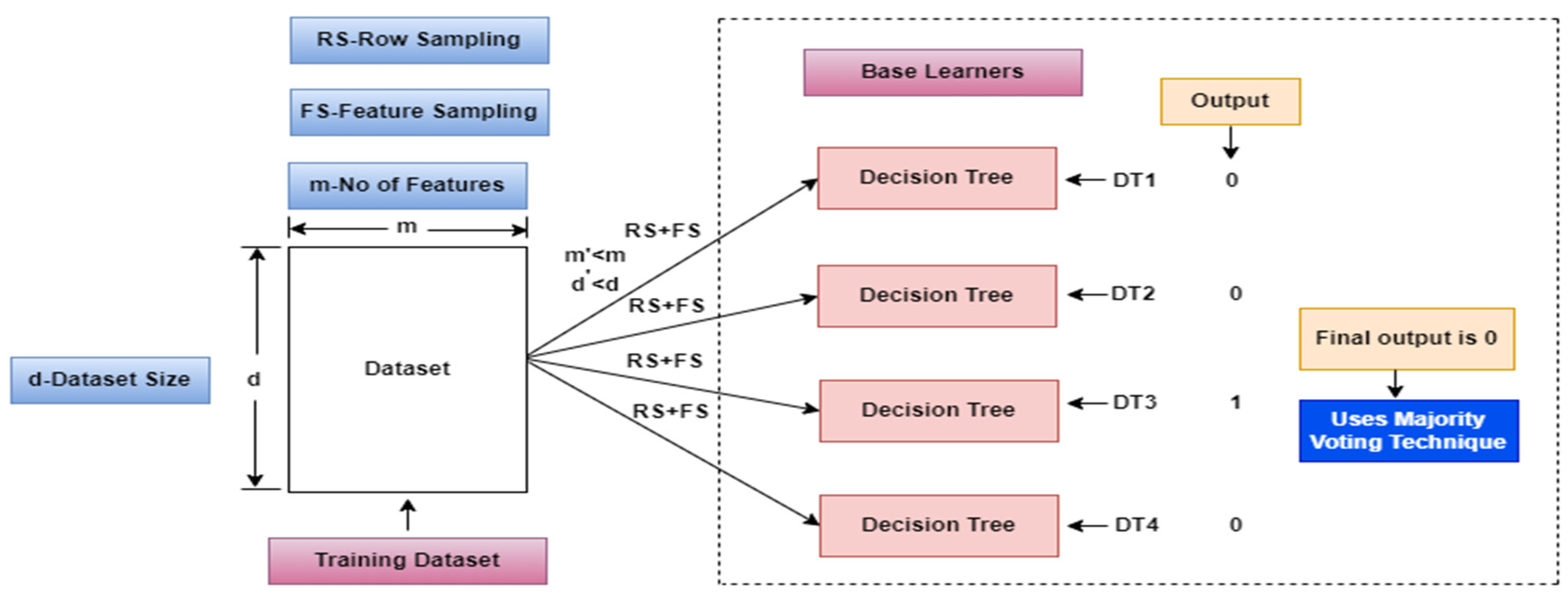
Figure 7.
Sentiment Spectrum (Mapping Positive and Negative Tweets).
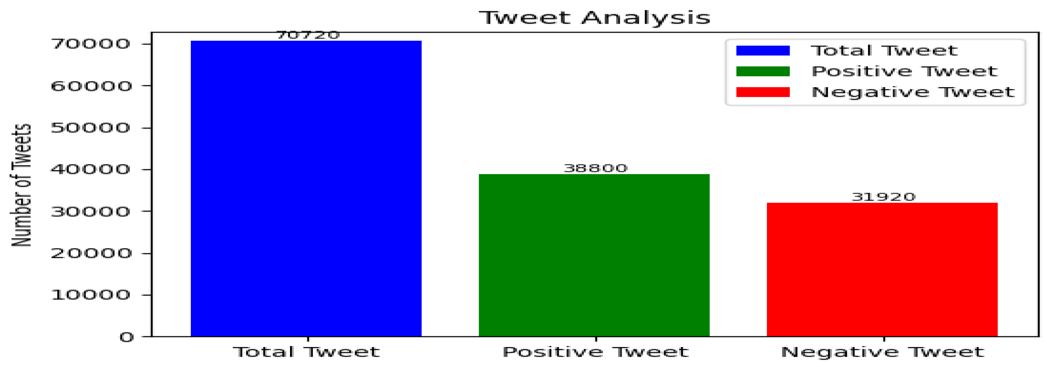
Figure 8.
Sample of the Employed Dataset after Pre-processing.
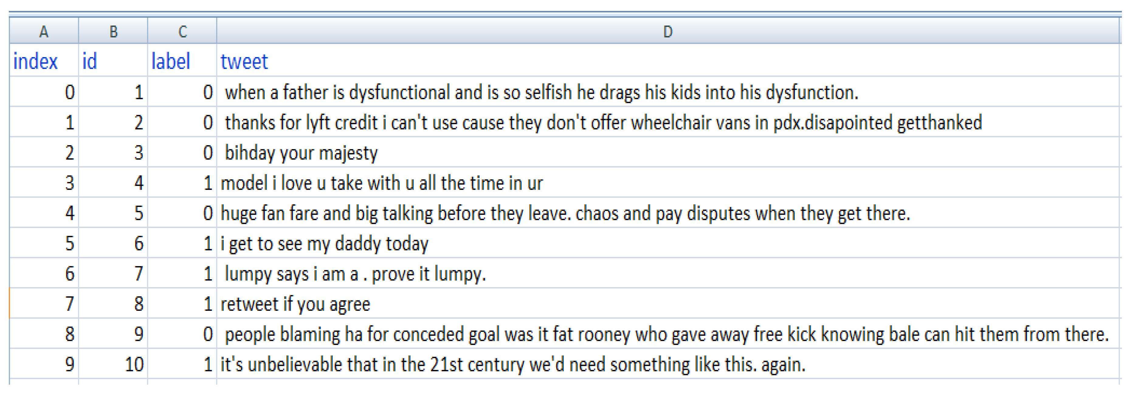
Figure 9.
Positive and Negative Wordcloud.
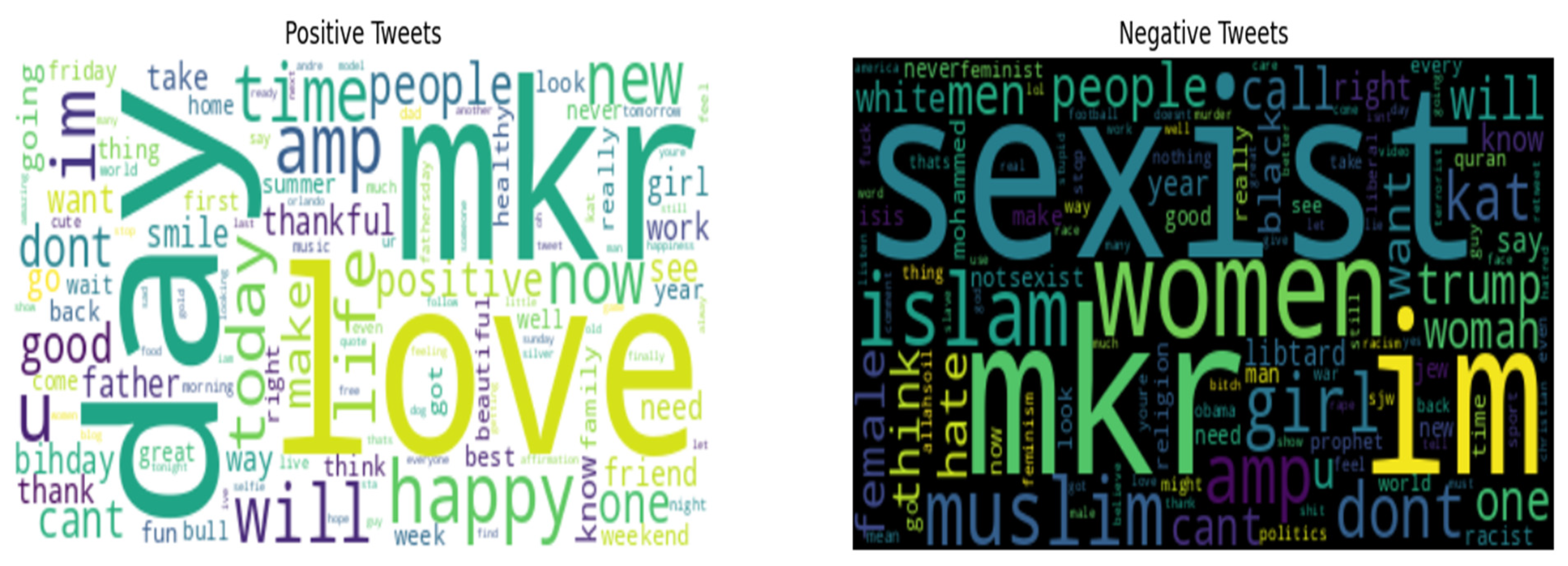
Figure 10.
(a). Comparative Analysis Based on Accuracy. (b). Comparative Analysis Based on Precision. (c). Comparative Analysis Based on Recall. (d). Comparative Analysis Based on F1-score. (e). Comparative Analysis Based on Specificity. (f). Comparative Analysis Based on ROC_AUC.
Figure 10.
(a). Comparative Analysis Based on Accuracy. (b). Comparative Analysis Based on Precision. (c). Comparative Analysis Based on Recall. (d). Comparative Analysis Based on F1-score. (e). Comparative Analysis Based on Specificity. (f). Comparative Analysis Based on ROC_AUC.
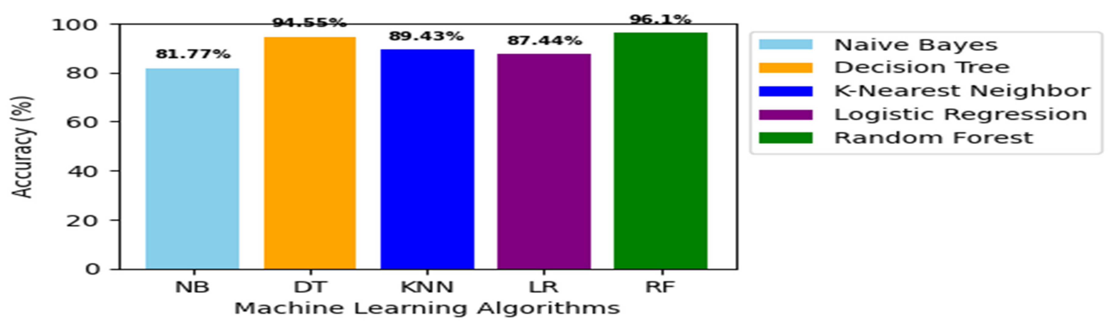
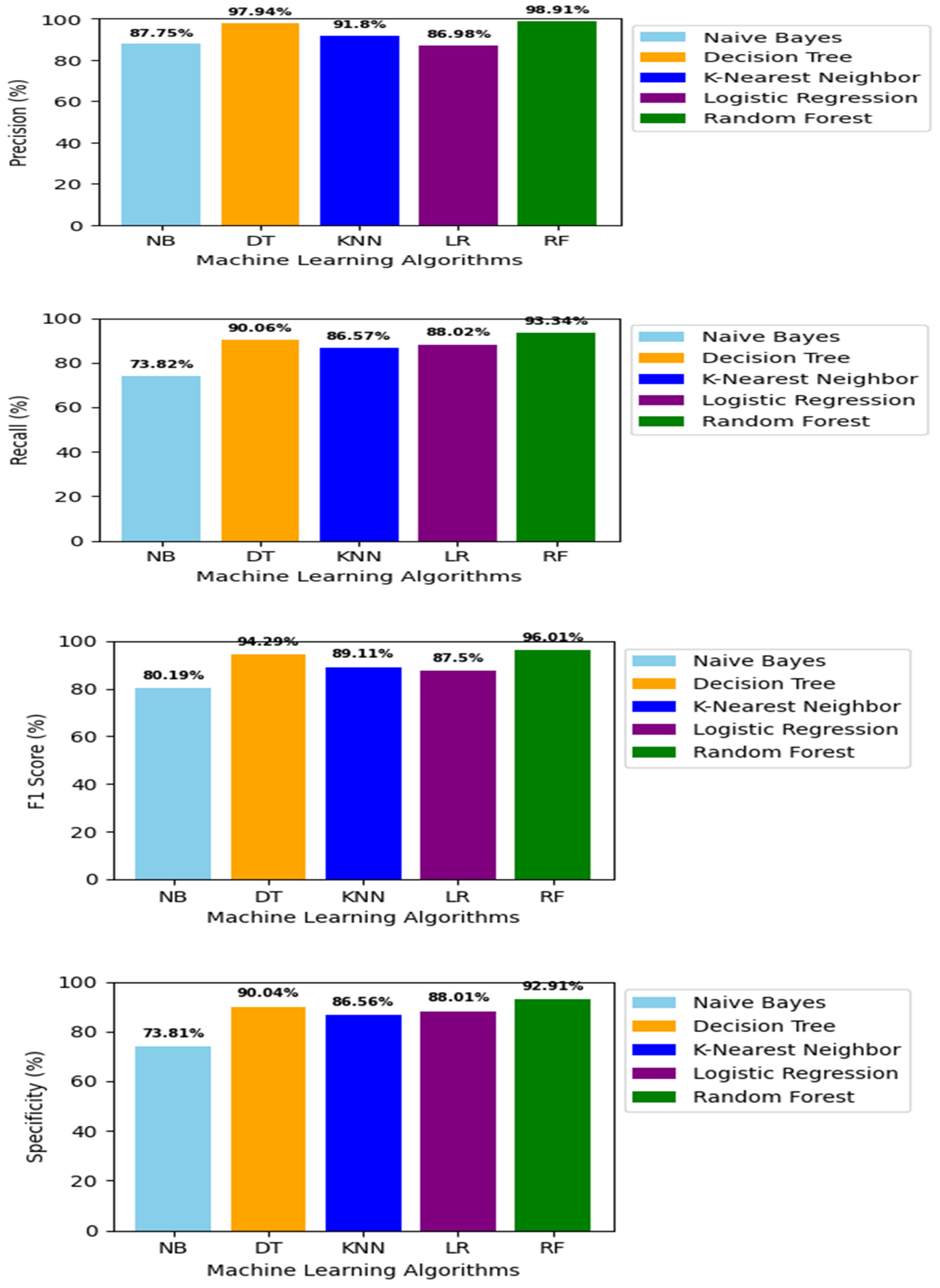
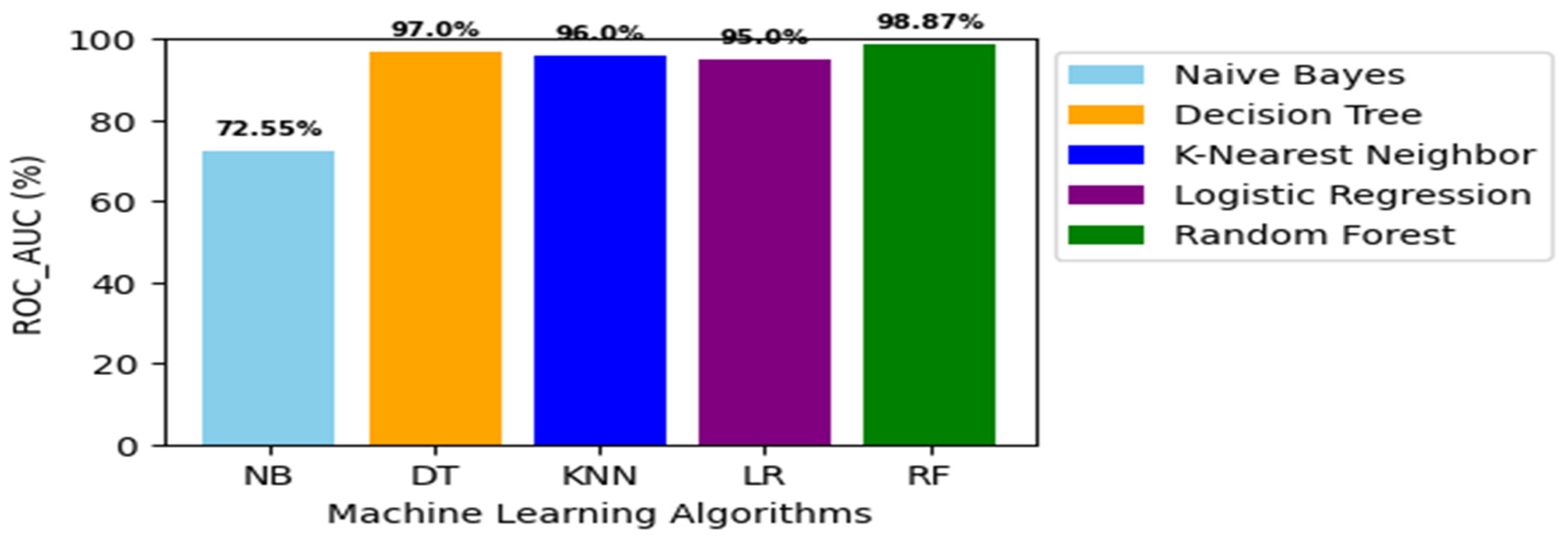
Figure 11.
(a). Confusion Matrix for NB Classifier. (b). Confusion Matrix for DT Classifier. (c). Confusion Matrix for KNN Classifier. (d) Confusion Matrix for LR Classifier. (e). Confusion Matrix for RF Classifier.
Figure 11.
(a). Confusion Matrix for NB Classifier. (b). Confusion Matrix for DT Classifier. (c). Confusion Matrix for KNN Classifier. (d) Confusion Matrix for LR Classifier. (e). Confusion Matrix for RF Classifier.
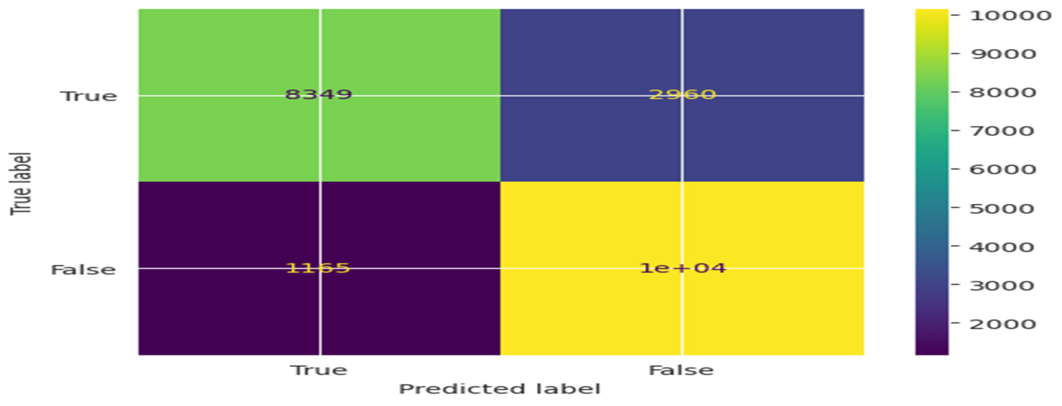
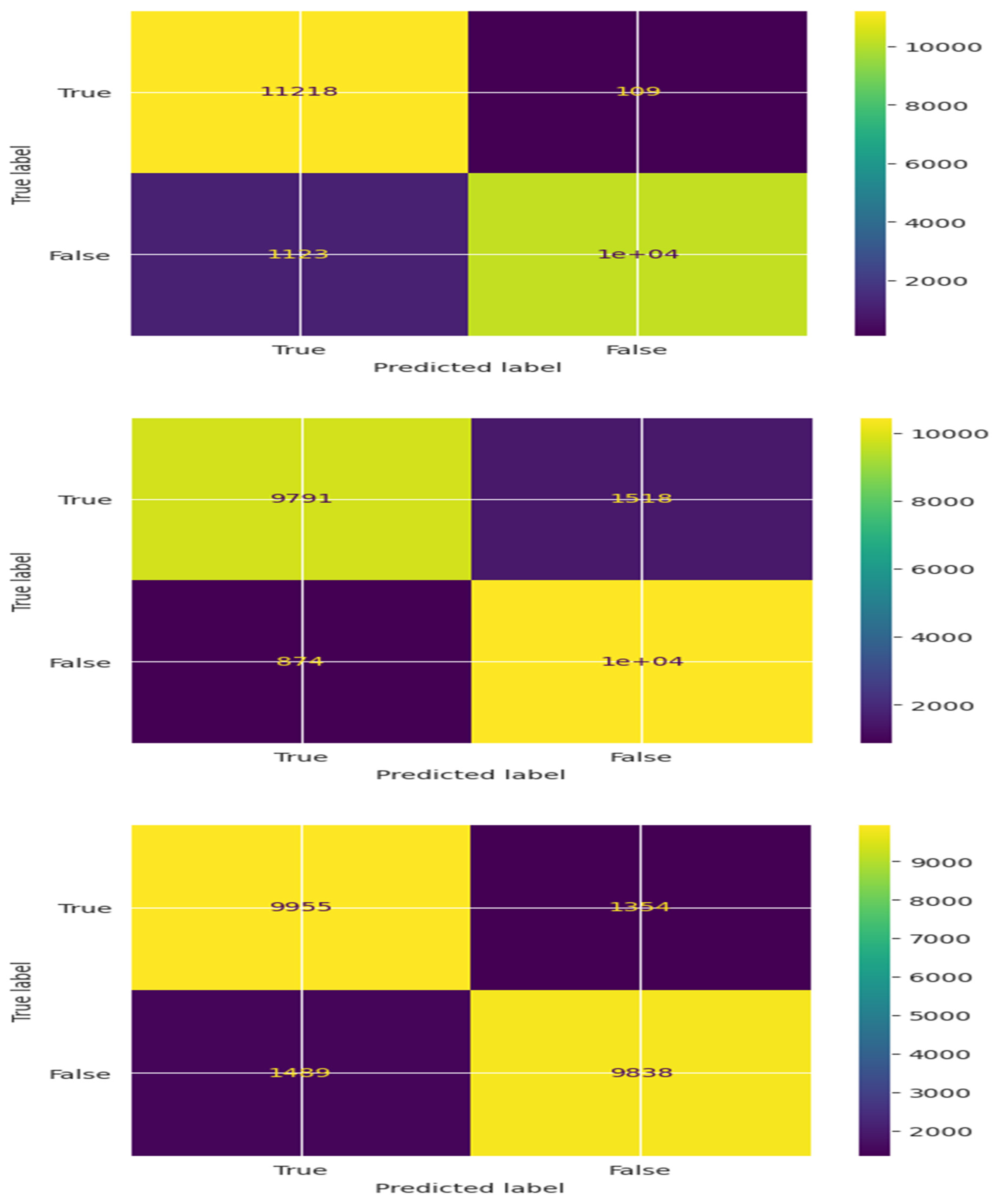
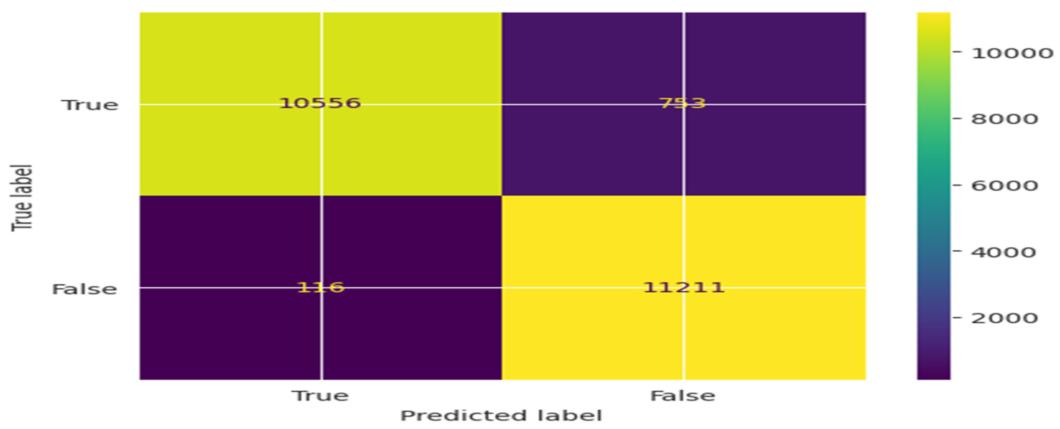
Figure 12.
(a). ROC curve for NB, DT, KNN, LR, and RF Classifier.(b). Precision-Recall curve for NB, DT, KNN, LR, and RF Classifier.
Figure 12.
(a). ROC curve for NB, DT, KNN, LR, and RF Classifier.(b). Precision-Recall curve for NB, DT, KNN, LR, and RF Classifier.
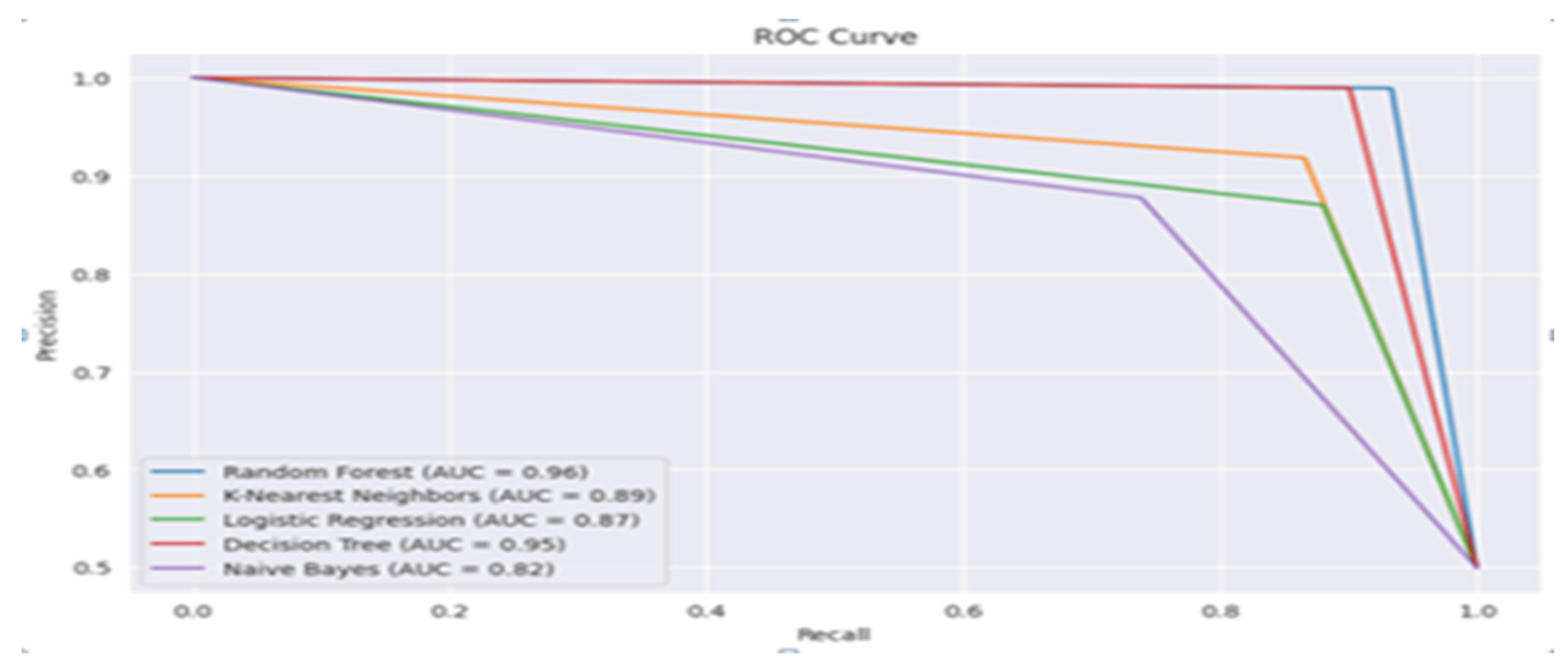
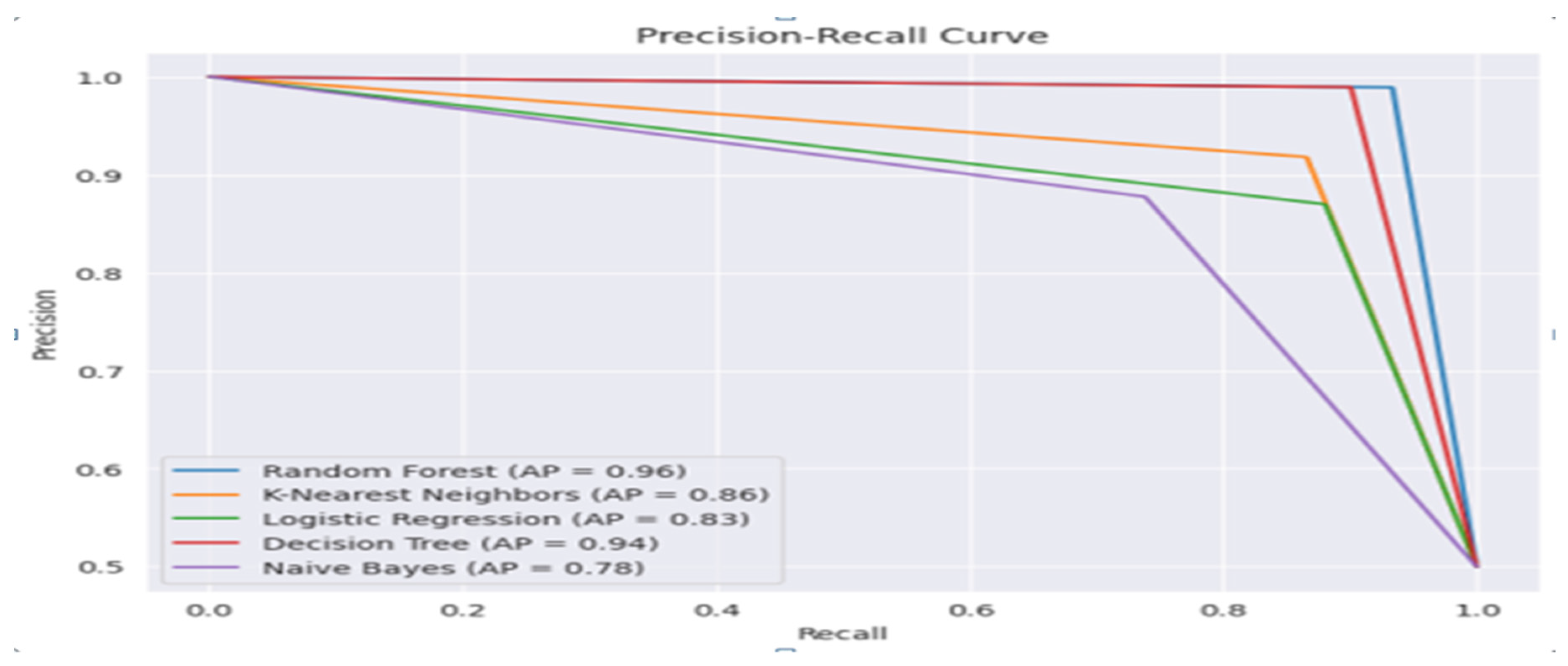
Table 2.
Algorithm Analysis and Metric Evaluation.
| Sl. No. | Methods used/ Reference | Vectorization Techniques | Performance Metric | |||||
| A | P | R | F1 | S | ROC_AUC | |||
| 1 | Logistic Regression [10] | Hashing vectorizer | 55.0 | 56.1 | 66.0 | 60.0 | - | 59.0 |
| 2 | Decision Tree (DT) [13] | Bag of Words (BoW) | 94.3 | 91.9 | 88.1 | 89.9 | 91.1 | - |
| 3 | Naive Bayes (NB) [14] | Count Vectorizer | 95.7 | 94.0 | 93.0 | - | - | 50.0 |
| 4 | Naive Bayes (NB) [15] | TF-IDF Transformer | 87.5 | 88.0 | 87.6 | 87.3 | - | 95.8 |
| 5 | K-Nearest Neighbor (KNN) [16] | Count Vectorizer | 92.4 | 92.3 | 92.5 | 92.8 | 91.8 | - |
| 6 | Support Vector Machine [17] | TF-IDF | - | 68.7 | 82.7 | 74.9 | - | - |
| 7 | Support Vector Machine with Particle Swarm Optimization (SVM-PSO) [18] | TF, TF-IDF | 77.0 | 77.5 | 76.1 | - | - | - |
| 8 | Support Vector Machine (SVM) [19] | Word2vec | 82.6 | - | - | 62.0 | - | - |
| 9 | Naïve Bayes [21] | TF-IDF | - | 94.6 | 94.64 | 94.62 | - | - |
| 10 | Proposed model (Random Forest) | CBow, Skip-gram | 96.1 | 98.9 | 93.3 | 96.0 | 92.9 | 96.1 |
Disclaimer/Publisher’s Note: The statements, opinions and data contained in all publications are solely those of the individual author(s) and contributor(s) and not of MDPI and/or the editor(s). MDPI and/or the editor(s) disclaim responsibility for any injury to people or property resulting from any ideas, methods, instructions or products referred to in the content. |
© 2024 by the authors. Licensee MDPI, Basel, Switzerland. This article is an open access article distributed under the terms and conditions of the Creative Commons Attribution (CC BY) license (http://creativecommons.org/licenses/by/4.0/).
Copyright: This open access article is published under a Creative Commons CC BY 4.0 license, which permit the free download, distribution, and reuse, provided that the author and preprint are cited in any reuse.


