
Submitted:
15 August 2024
Posted:
15 August 2024
You are already at the latest version
Abstract
The drinking water temperature is expected to increase in the Netherlands due to climate change and the installation of district heating networks as part of the energy transition. To determine effective measures to prevent undesirable temperature increase of the drinking water a model is developed. This model describes the temperature in the drinking water distribution network as a result of the transfer of heat from the climate, above and underground heat sources through the soil. The model consists of two coupled applications. The extended soil temperature model (STM+) describes the soil temperatures, in a two-dimensional finite element method that includes a drinking water pipe and two hot water pipes, coupled to a micro meteorology model. The extended water temperature model (WTM+) describes the drinking water temperature as a function of the surrounding soil temperature (the boundary temperature, resulting from the STM+), thermal sphere of influence where the drinking water temperature influences the soil temperature, and the hydraulics in the drinking water network. Both models are validated with field measurements. This paper describes the WTM+. Previous models did not consider the cooling effect of the drinking water on the surrounding soil, which led to an overestimation of the boundary temperature, and to an overestimation of how quickly the drinking water temperature reaches this boundary temperature. The field measurements show the improved accuracy of the WTM+ when considering one to two times the radius of the drinking water pipe as the thermal sphere of influence around the pipe.
Keywords:
drinking water temperature
; water quality
; model validation
1. Introduction
During transport and distribution, the drinking water temperature can increase due to relatively high soil temperatures surrounding the drinking water distribution network (DWDN). A drinking water temperature below 25 °C at the tap is required to meet Legionella prevention standards and/or drinking water standards [1]. Soil temperatures are affected by climatic factors and anthropogenic heat sources above and below ground level [2,3]. With climate change, urbanisation, and the energy transition, which in the Netherlands in particular comes with an expected increased number of district heating networks (DHN), the urban subsurface will heat up even further. Currently the drinking water temperature at the tap sporadically exceeds the norm, but with these developments more exceedance is expected [1].
As pipes in the DWDN typically can last for more than 100 years and modifications during this lifetime are expensive, measures to prevent high drinking water temperature should be taken in the coming years, well in advance of temperatures rising to problematic levels. To understand the effectiveness of various measures to keep the drinking water temperature at the tap below the threshold, a modelling approach is followed. Such a model requires the possibility to model a highly meshed DWDN a) in which flows are constantly changing; b) with various boundary conditions of the produced (incoming) drinking water temperature which depends on the season; c) with various boundary conditions of the soil temperature around the DWDN which depends on the season and underground heat sources such as DHN, and d) that leads to accurate drinking water temperatures thus allowing to determine effective measures to keep the drinking water temperature below the threshold of 25 °C. Blokker and Pieterse-Quirijns [2] developed an approach with a one-dimensional soil temperature model (STM) and a drinking water temperature model (WTM). The WTM calculates the drinking water temperature at each customer based on a hydraulic network model (requirement a) and heat exchange between the soil around the pipe wall and the drinking water (requirement b), where the soil temperature is calculated by the STM. The STM was first developed (and validated) for the soil temperature of the shallow underground in an urban environment (i.e. in sand and under tiles). It was then expanded to include weather forecasts [4], other soil types (peat, clay with their specific heat exchange properties), other soil covers (grass, trees) and generic anthropogenic heat sources [3]. The STM does not allow for modelling a specific anthropogenic heat source such as a DHN (requirement c). The WTM was validated in a DWDN at locations with large residence times, allowing to validate that the drinking water reaches the soil temperature, but not the rate at which this happens, and therefore it is not clear if temperatures in the entire DWDN are determined accurately (requirement d). When one wants to estimate the importance of specific influences on the drinking water temperature (e.g., climate change, DHN or countermeasures), it becomes important to validate the WTM also over its temporal scale.
The WTM assumes a constant temperature at the outer pipe wall disregarding that - in reality - heat exchange between the drinking water and the soil will also affect the soil temperature within a certain sphere of influence. Various authors have suggested to add an insulation layer of soil around the DWDN in a WTM-like approach [5,6,7]. Each suggested a different approach to determine the insulation layer thickness. The validity of their approaches is unclear, as two of them [5,7] were only theoretical approaches. The third one [6] did validate the model against measured water temperatures, but as the model included heat loss at consumers it is unclear how impactful their approach to include conductive and convective heat resistance of the soil is. Hypolite et al. [8] showed that good estimates of the drinking water temperature can be obtained for a system of large transport mains when the role of the soil in heat transport is considered. Models for water temperature in underground networks are also used to determine heat losses in a DHN [9,10,11,12,13,14]. For DHN a simple modelling approach without explicitly incorporating an insulation layer of soil around the network suffices. Firstly, the heat losses at the consumers are more substantial than the heat loss in the network, and secondly the temperature differences between the soil and the water in the DHN are large and in order to get a good estimate of the order of magnitude of the heat losses the heat exchange with the soil does not need to be known with a high accuracy.
The time it takes for the temperature in the soil around a drinking water main to change, is in the order of days to weeks. The time it takes for the temperature of the drinking water to change is in the order of minutes to hours. As these temporal scales differ a lot, it was decided to stick with the approach of two models. Both models were improved, leading to: 1) an enhanced STM [called STM+, 15] which calculates the soil temperature profile as it is influenced by both drinking water temperature and external influences such as DHN and the weather; 2) an enhanced WTM (called WTM+) which calculates the drinking water temperature as it is influenced by the soil temperature as calculated by the STM+. The time scale of the WTM+ is typically hours; the time scale of the STM+ is typically months. The result of the STM+ is a soil temperature that is used as a boundary condition of the WTM+.
The STM+ is described and validated; the reader is referred to van Esch [15]. In the present paper we describe the WTM+, in particular how the thermal sphere of influence is modelled. To show that the WTM+ has improved with respect to the WTM a proper validation is essential. We show a validation of the model with two cases. The first case is a single pipe of ca. 1 km long with a variation in residence times. The second case is a DWDN where half of the network is potentially influenced by a DHN, and the other half is not.
2. Materials and Methods
2.1. The Water Temperature Model (WTM+)
The change in water temperature, Twater, due to heat transfer (during contact time t) between the surroundings and the flowing water in a pipe can be described as [2,16]:
where Tboundary is the temperature which the drinking water will eventually reach, and k is the heat transfer rate (1/s). In the modelled system, Tboundary is assumed to occur at some distance from the pipe wall (section 2.2 discusses how to determine Tboundary) and k depends on that distance, and on the characteristics of the water, pipe material, pipe surroundings, and on the hydraulic characteristics of the water flow. Specifically, k is given by [2,17]:
With D1 the inner pipe diameter (m), D2 outer pipe diameter (m) and D3 the diameter where the boundary condition T = Tboundary is applied (m). The dimensionless Nusselt number, Nu, summarizes the hydraulic conditions of the system and – for pipes – can be described as a function of the dimensionless Reynolds number (Re) and Prandtl number (Pr): Nu = 0.027 Re0.8 Pr0.33 for turbulent flows (Re > 10.000), and Nu = 3.66 for laminar flows (Re < 2,300). Furthermore, αwater is the thermal diffusion coefficient [0.14·10-6 m2/s]; αwater = λwater/ρwater Cp, water; λwater is the thermal conductivity of water [0.57 W.m-1.K-1]; ρwater is the density of water [1000 kg.m-3]; Cp,water is the heat capacity of water [4.19·103 J.kg-1.K-1] – with the parameter values given at 20 °C. In this paper, we only consider plastic pipes, for which λpipe is the thermal conductivity of PVC [= 0.16 W.m-1.K-1]. We typically consider pipes that are installed in sand, for which λsoil is the thermal conductivity of dry sandy soil [= 1.6 W.m-1.K-1].
With the time-dependent boundary conditions Twater(τ=0) = Twater,0 and T(τ=∞) = Tboundary, the analytical solution for this is:
where t is time and τ is the contact time (in drinking water context, this is the residence time). Note that k can also be time dependent, e.g. when hydraulic conditions change over time. Eq. (1) to Eq. (3) derive from Fourier’s heat equation, describing how Twater changes over time during transport through the network, with the local difference between Twater and Tboundary as the driving force for local heat transfer. A central assumption is that the temperature profiles in the pipe wall and the surrounding soil are developed into a steady state. This assumption is reasonable if the drinking water temperature changes much faster than the soil temperature profiles.
Figure 1 visualizes how the equations and boundary conditions of the current model (Figure 1b and Figure 1c) and those of its predecessor (Figure 1a) approximate the temperature profile in the modelled system:
- Figure 1a (the left panel) shows the situation as modelled by the original WTM, where a constant soil temperature is applied directly onto the outer pipe wall (green dot), i.e. R3 = R2. No gradient in the soil temperature profile is considered.
- Figure 1c (the right panel) shows one first possible approximation of the presented approach. When heat is exchanged between soil and water, a soil temperature profile develops with a gradient that attenuates with increasing distance from the pipe. The blue lines and green dots show the profile that develops around a pipe in which the water temperature is kept constant for a long time, as modelled with the STM+. This profile could be taken as input for the WTM+ by using the Tsoil and R of any of the green dots to determine Tboundary and D3 (dotted red lines). If a Tboundary of 26.5 °C is used, like in the other panels, that requires a D3 corresponding to an R of approximately 1400 m (not shown).
- Figure 1b (the centre panel) shows a presumably more realistic approximation with the presented approach. Contrary to the assumptions of the previous two figures, the temperatures of both the water and the pipe surroundings may change over time at any one specific location along the network. As a result, it is unrealistic to expect the fully developed temperature profiles of Figure 1c. Instead, a dynamic profile between fluctuating soil and water temperatures should be expected, represented by the dotted blue lines. If a semi-steady state can be assumed for this profile, it could be modelled with the WTM+ by applying the temperature Tboundary at some distance R3 (the radius corresponding to D3 in the equations) of the pipe (green dot) in a way that the slope of the profile is best approximated. The true temperature profile will not be discontinuous at R3, so the temperature profile that follows from Eq. (1) to Eq. (3) (red lines) does not perfectly describe the realistic situation.
In each panel of Figure 1, the model behaviour is shown for three different values of Twater. These three temperatures can be imagined as occurring over the length of the pipe as the drinking water travels through the network. This means that, after a certain time t, the drinking water will have travelled a certain distance x, and the drinking water temperature will then have increased under the influence of the Tboundary assumed for the surrounding soil (26.5 °C in this example). For Figure 1a, the temperature gradient for any given water temperature is much steeper (and thus heat exchange is faster) than for Figure 1b. The example temperatures will therefore be reached at different moments in time, which is why different suffixes are used to indicate the time. The situation in Figure 1a - the old WTM - will lead to an overestimation of how quickly drinking water will be heating up compared to the actual situation, because heat transfer is never decreased by development of a less steep temperature gradient in the soil. The situation in Figure 1c will lead to an underestimation of how quickly drinking water will be heating up compared to the actual situation, because the exaggerated removal of heat for the soil by water with a constant temperature leads to overly attenuated temperature gradients and heat transfer in the soil.
Applying a Tboundary at a distance D3 in the WTM+ should be considered a mathematical approximation to compensate for the fact that we haven’t built one integrated model but couple two models (WTM+ and STM+) while the boundary conditions of the two are not fully independent. Eq. (2) assumes that D3 is constant over time, and Eq. (3) assumes that D3 and Tboundary are constant over the residence time t (i.e. constant over the pipe length). Tboundary is determined with the STM+, see Section 2.2.
In practice, the value of D3, the distance at which a constant Tboundary can reasonably applied, is not known a priori. In this paper we try to estimate the value of D3 from measurements of Twater at various distances and residence times (t0, ty, ty’) and estimates of Tboundary (using the STM+) in two case studies (Section 3 and Section 4). Various authors [5,6,7] suggested values for D3 related to the pipe installation depth. However, it is unclear which approach works best, partly due to a lack of validation. We expect that the value of D3 is most likely larger for large pipe diameters than for small pipe diameters, with a large body of water having more potential to influence the soil around the pipe. To make this scaling influence of the pipe diameter more explicit, we introduce the thermal sphere of influence (TSoI) as an explicit scaling factor: D3 = D2 + 2×TSoI×D1.
2.2. Tboundary from the Soil Temperature Model (STM+)
Tboundary in Eq. (1) is the temperature which the drinking water will eventually reach, and this takes place when the soil and drinking water temperature are in a (dynamic) equilibrium. This equilibrium temperature (Tboundary) may be different from the undisturbed soil temperature, and therefor is determined with the STM+. For a thorough description of the STM+, including its validation, the reader is referred to van Esch [15].
The STM+ input parameters are a time series of atmospheric circumstances (temperatures, radiation, etc., a so-called micrometeorology model), type of surface (tiles, grass, trees), type of soil (dry or wet sand, clay), and evaluates heat transfer for a 2-dimension geometry which includes a drinking water pipe. The STM+ calculates soil temperatures in a large grid around the drinking water pipe. The temperatures around the pipe are not constant. Instead, the average temperatures over the circumference of circles around the pipe wall (at a distance of one to two times D2) were reported as relevant for determining Tboundary. The STM+ average temperature is referred to as “the” soil temperature at a certain distance from the pipe wall (Tsoil).
The STM+ can be operated in the so called “passive” and “active” mode.
- In the passive mode, the drinking water temperature is a simulation result and not a boundary condition, i.e. Tsoil influences the drinking water temperature, but not vice versa. It was shown that Tsoil is practically constant over the distance from the pipe wall (up to 3 × D2, or TSoI = 0.2 to 1), and equal to the calculated Twater. This by definition is Tboundary. van Esch [15] showed that Tboundary from the STM+, passive mode is equal to Tsoil from the STM, so equal to the undisturbed soil temperature. Note that this mode is used in the left panel of Figure 1.
- In the active mode, a constant drinking water temperature is imposed, which means the drinking water is acting as an infinite heat source. van Esch [15] showed that in this case Tsoil can be described as a function of the distance from the pipe wall (up to TSoI = 1) and Twater, 0. Plus Tboundary, defined as the temperature that is reached when soil and drinking water temperature are in balance, can easily be determined and is practically independent of this distance from the pipe wall (up to TSoI = 1). Note that this mode is used in the right panel of Figure 1.
This means that the STM (or STM+ passive mode) combined with the WTM (or WTM+ with D3 = D2) reflects the situation of stagnant drinking water. The STM+ active mode combined with the WTM+ reflects the situation where the drinking water at a certain location in the pipe is continuously refreshed and kept at a constant temperature and there is an equilibrium with the soil temperature. This is mimicking water flowing at a constant flow rate, where the soil temperature along the pipe is constant. In a typical drinking water distribution main, the flow rate changes over the day with (almost) stagnant water during the night and high flow rates during peak hours. The conditions are therefor never equal to the ones in the passive nor in the active mode. Furthermore, the two modes lead to a different value for Tboundary; van Esch [15] showed that for summer conditions the passive mode leads to a slightly higher value than the active mode. This means that in the case studies in this paper the coupling between STM+ and WTM+ is not obvious, i.e. both D3 and Tboundary are unknowns.
2.3. Model Normalisation for Validation
In case study 1, the measurements are done over a few weeks, and the boundary conditions Tboundary and Twater 0 are not constant over this period, with a maximum change of 1.0 °C per 24 hours. We assume that k in Eq. (3) is constant during each test at a specific (constant) flow rate, and from it we want to determine the value for D3. In order to be able to do this, we are rewriting Eq. (3), assuming that at each time t during each test, the equation is valid. The model is normalized across tests with and :
The normalized temperature difference ΔTN represents the change in temperature of the drinking water along the pipe length relative to the difference in drinking water temperature and the surrounding soil, which we refer to as the driving force. The result is graphically shown in Figure 2 for various values of D1 and D3, where ΔTN = 0 represents Twater(τ) = Twater,0 and ΔTN =1 represents Twater(τ) = Tboundary, even when the boundary conditions are not constant.
2.4. Case Studies
The validity of the approach of the WTM+ to model the drinking water temperature over the length of a pipe with Tboundary from the STM+ and a layer of soil as an insulator (TSoI) needs to be verified. This will be done in two case studies: the first case study is a single pipe with an internal diameter of 152 mm and the second one is a DWDN where most pipes have an internal diameter of 100 mm. Case study one had limited spatial variation, where a lot of parameters were well defined, but had significant temporal variation; case study one had limited temporal variation, but significant spatial variation with some unknow parameter values. As the value of the TSoI is not yet known, the case studies will also be used to estimate its value. This means that the case studies are used both for validation and calibration.
For both case studies a sensitivity analysis was done (reported in appendices B.3 and C.3), and measurements were taken for validation and calibration. Details are described per case study in their respective sections below.
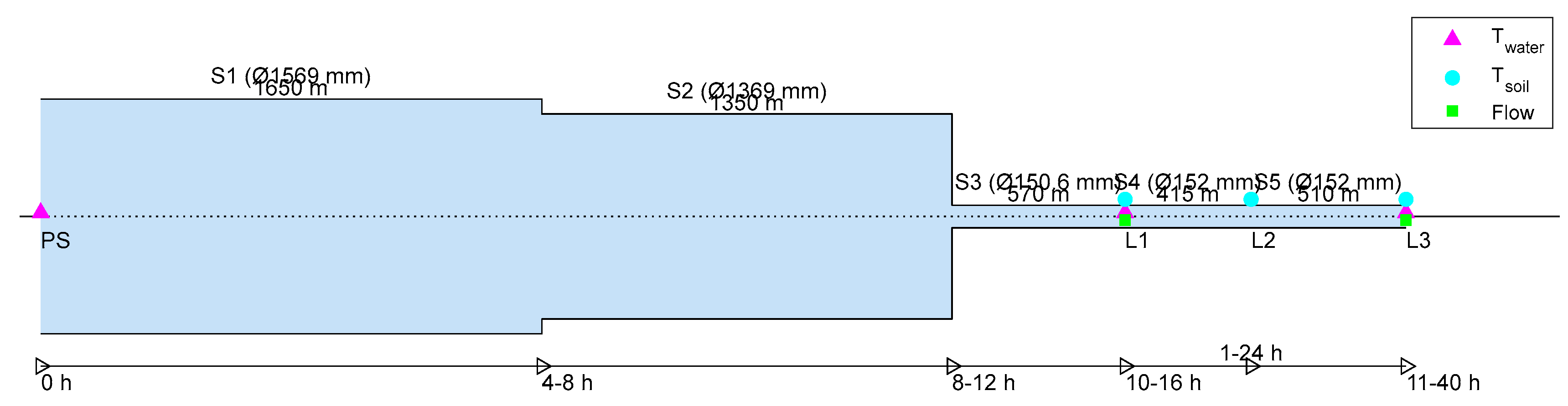
3. Case 1 - Single Pipe, Ø160 mm PVC
3.1. Case Study Description
A 925 m long Ø160 mm PVC pipe (D1 = 152 mm, D2 = 160 mm) in Rotterdam with only a few connections along the pipe stretch was selected by Evides water company and KWR for the validation of the WTM+ (and the STM+). This pipe is fed from a surface water PS (pumping station) through 3 km of large diameter mains (PVC > 1350 mm internal diameter) and a smaller branch of 570 m (internal diameter 150,6 mm). It is assumed that the temperature at the start of this branch is equal to the temperature from the PS (ΔTN < 0.05 after 4 hours, for Nu = 100 (turbulent flow), PVC DN1400, and D3 = 0). The end of this branch is the first location (L1) of the case study. The water in the case study pipe flows from location L1 to L2 (415 m) to L3 (510 m). For this pipe, taking the example of Figure 1, the required residence times (for turbulent flows) can be estimated as tx ≈ 1 h, tx’ ≈ 8 h, ty ≈ 3 h, ty’ ≈ 24 h, tz ≈ 9 h, tz’ ≈ 61 h. This means measurements are focussed on residence times between 1 and 24 hours.
For the single pipe a sensitivity analysis for was done analytically, see B.3. It shows that and are the most influential parameters. And there is a distinct difference between turbulent to laminar flows.
The drinking water temperature was measured at the PS, L1 and L3. The flow between L1 and L3 was controlled with a hydrant at L3 and measured. During a two weeks period (18 May 2020 – 03 June 2020) the flow rate was controlled such that residence times of the water in the pipe from 1 to 24 hours were obtained, see Table B1. At the same time, soil temperatures were measured at various distances from the pipe wall at locations L1, L2 and L3, which were used to validate the STM+ [15]. The values for input parameters used in the WTM+ (Eqs. (2) and (4)) are shown in Table B2. Appendix B.1 has more information on the test location, including a schematic overview.
During the measurements there was practically no demand from customers along the pipe, as there is only one residential customer, and some sports facilities which were closed during the Covid-19 pandemic. The demand at the customer location was measured, and it had a negligible effect on the flow at L1. The logging frequency for flow and temperature measurements was once per 15 minutes. The residence time between L1 and L3 was calculated from the pipe length, pipe diameter and flow.
Tboundary was estimated with the STM+ [15] results for L3, where detailed info on the actual soil parameters was used. The STM+ was validated on this particular case study, and then the model was rerun in the so-called passive mode and active mode (See Section 2.2), both for laminar and turbulent flows. Tboundary for stagnant water (STM+ passive mode) was 0.3 to 0.9 (on average 0.7) °C lower than Tboundary for turbulent flowing water (STM+ active mode, Nu = 3.66) and 0.2 to 0.7 (on average 0.5) °C lower than Tboundary for laminar flowing water (STM+ active mode, Nu = 100).
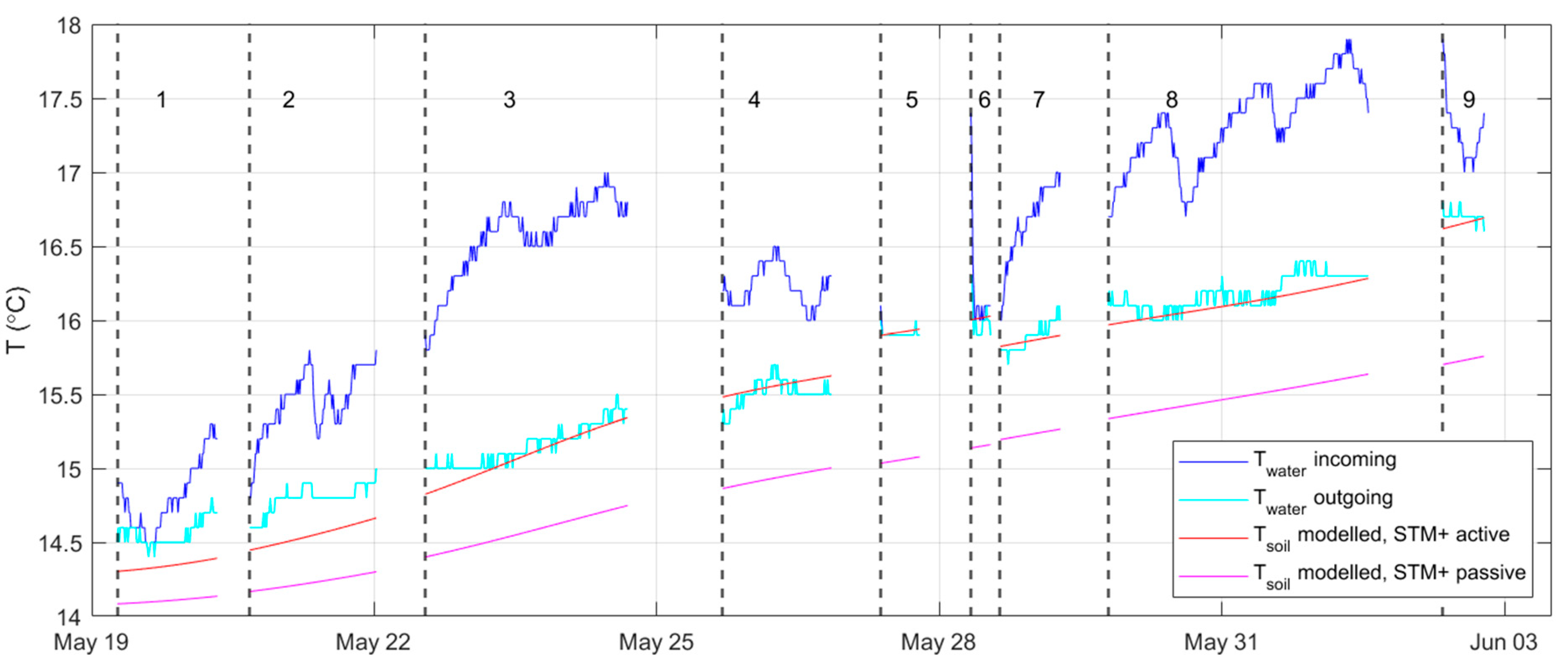
Figure 3 shows the measured and modelled temperatures. During each test the flow was kept constant. After a certain time (and with constant incoming drinking water temperatures), a dynamic equilibrium as in the situation simulated in the STM+ active mode could be expected. However, the constant flow was only imposed for a relatively short time, viz. 5 hours to max 66 hours (Table B1), and the incoming water temperature was not constant (Figure 3). This means that it isn’t obvious which STM+ (passive or active mode for turbulent or laminar flows) would be applicable. The small differences in Tboundary for this case study will have a significant effect because the difference between incoming and outgoing water temperatures and soil temperatures are relatively small (< 2.0 °C). As it is unclear which is the “true” Tboundary, both STM+ modes are tested.
It is required to do some data processing to validate the WMT+ with these measurements (Appendix B.2). A normalization step was done because none of the parameters in Eq. (4) are constant over time. Also, due to measurement accuracies some data was excluded (22 datapoints where the drinking water temperature between beginning and end of pipe seemed to change in the opposite direction compared to the soil temperature; 93 datapoints where the uncertainty was too large). As a last step, the individual datapoints with similar residence times were grouped and shown in boxplots.
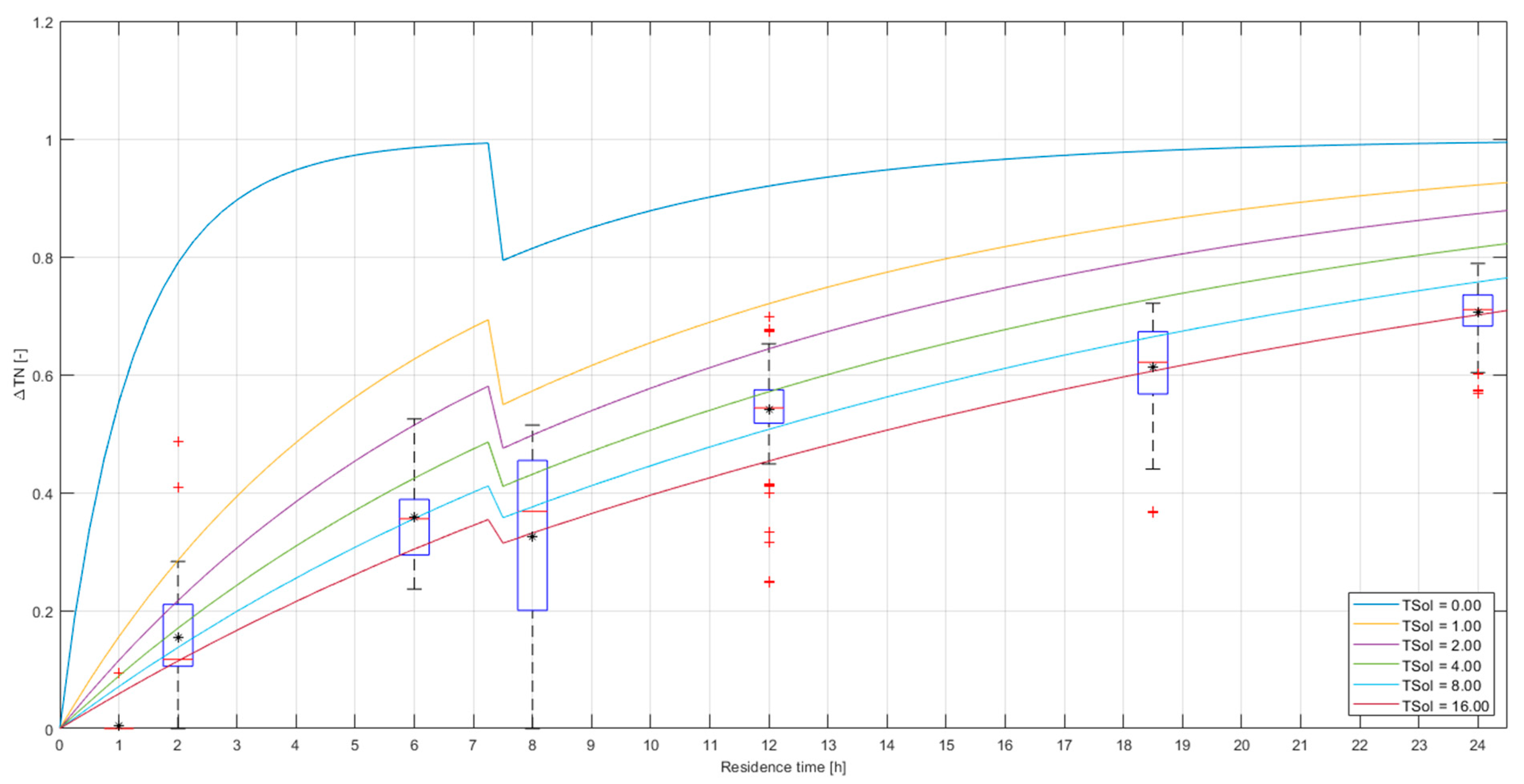
3.2. Case Study Outcomes and Discussion
Figure 4 shows ΔTN versus residence time with the measurement in boxplots and theoretical lines for various values of TSoI. The measurements at 1 and 2 hour residence times were mostly discarded because of large measurement uncertainties. After filtering there are no datapoints left with negative values, but there are still a few datapoints that are larger than 1. These are mainly found in test 4 (with a 12 hour residence time).
The theoretical lines depend on the Nusselt number, with a low Nu in the laminar flow regime and a high Nu in the turbulent flow regime. Typically the literature suggests laminar flows at Re < 2,100-2,300, but turbulent flows can start to occur anywhere at Re > 3,500-10,000 [18]. Figure 3 shows that at the start of tests 5, 6 and 9 the incoming water temperature changes very quickly with about 0.5 °C in the first few hours; this is not the case for the other tests. This may suggest that for the high flow tests there is turbulent flow in the pipe upstream of L1, and therefore (same pipe diameter, but slightly different flows) probably also between L1 and L3. For residence times of 8 hours and more we may assume laminar flows. In this case study a residence time of 7 hours means Re ≈ 5,000.
Figure 4 shows that the variability is large compared to the average values. It can be roughly estimated that the data correspond with values of TSoI between 0.0 (blue line) and 1.0 (purple line). As the variability of the data covers multiple theoretical lines it is impossible to determine with enough certainty what the correct value of TSoI is.
Using Eqs. (1) and (2), the TSoI was calculated for each datapoint over the duration of each test. Figure 5 shows that the value for TSoI sometimes changes gradually over time, and sometimes the change is more abruptly. The spikes in the changes are explained by the inaccuracies of the measurements. To illustrate this, we zoom into test 3. Figure 3 (or more clearly in Figure B3) shows that Twater, 0 increases gradually from 15.8 to 17 °C, although due to the 0.1 °C accuracy it doesn’t look very gradual. The same can be said for Twater (t) increasing from 15 to 15.5 °C. Tboundary increases from 14.8 to 15.3 °C. The difference between Twater (t) and Tboundary is typically less than 0.1 °C, or, given the measurement inaccuracies, the difference is between 0 and 0.2 °C. In Eq. (4) this means that the denominator and the numerator are the same plus or minus 0.2 °C, or ΔTN ≈ 1. At first Twater (t) - Twater, 0 = 1.0 °C, or ΔTN = 0.8 - 1.2, and after 24 hours Twater (t) - Twater, 0 = 1.5 °C or ΔTN = 0.9 - 1.1. This explains the relatively large spikes in TSoI, with a decrease over time. The values smaller than 0 have no physical meaning and can also be explained with the uncertainty in the parameters of Eq. (4). Figure 5 thus clearly illustrates the effect of measurement uncertainty. As (Twater,0 – Tboundary) ≈ 0.6 to 1.6 °C during the test period (Figure B3), it can be shown that it is impossible to have highly accurate results where (Twater - Tboundary) > 0.2 °C. From calculations it follows that if D3 = D2 (TSoI = 0), (Twater - Tboundary) would be smaller than 0.1 °C for all tests, except for test 1 (0.13 °C). Even if D3 >> D2 (e.g. TSoI = 20), (Twater - Tboundary) > 0.1 °C only for tests 1, 2, 4, 7 and 9. Note that (Twater,0 – Twater) > 0.5 °C for all tests. This means that for the TSoI we should consider the average of the calculated values; the instantaneous values are not reliable enough.
Figure 5 also shows a decrease in TSoI over time. The tests at 18.5 and 24 h residence time have a TSoI of 1 to 3 at the start of the test, and a TSoI of 0 to 1 at the end. The test at 8 h (test 1) and the first test at 12 h (test 2), i.e. the first two tests, show higher values (TSoI = 1 - 2) than the later tests (tests 4, 7 and 9 with TSoI ≈ 0).
The same data processing was done with Tboundary from the STM+ passive mode calculations. The results are shown in Figure B5. In these calculations less data points were discarded, because was larger. However, the uncertainty due to is still significant. This exercise leads to estimates of TSoI = 5-10, where under none of the imposed residence times Twater (almost) equals Tboundary. The results from the passive mode are put into the Suppl. Mat. Section, because in case study 2, TSoI values are found that are much closer to the ones from the results of the active mode.
4. Case 2- Drinking Water Distribution Network
4.1. Case Study Description
Case study 2 for the validation of the WTM+ consisted of drinking water temperature measurements done on 31 August 2020 in the DWDN of Almere. The Almere DWDN, owned and operated by Vitens, is ca. 700 km long, consists mainly of PVC pipes, with nominal diameters of Ø63 (8%), Ø110 (51 %), Ø160 (15%), Ø200 (5%), Ø310 (6%) and > Ø400 mm (9%) (more info in [19]). The DWDN is fed by two feeding reservoirs, in the north and in the south part of the system that are referred to as F1 and F2 (Figure 6). The drinking water temperature were = 13.7 °C and =13.3 °C on 31 Aug 2020, respectively. Limited variation in these temperatures is expected over the duration of the test (less than a day) as this is drinking water from a ground water source.
The drinking water temperature was measured by Vitens employees at 35 locations on hydrants (see Figure 6) at two moments of the day (one between 8:00 and 12:30, and one between 12:45 and 16:30) leading to a total of 70 data points. During the tests the hydrants were opened with a low flow. Two areas (area A and B, see Figure 6) were selected for the temperature measurements. Note that according to Figure 2, these times should show a distinction in drinking water temperature changes for 110 mm pipes. The two areas have a similar year of installation and thus a similar design philosophy (with similar pipe diameters, materials, and network layout) and a similar number of residents. They have a comparable residence time from the sources. The two areas are likely to differ in soil temperatures (see Table C3). The pipes in areas A and B are at different installation depths and in different soil types. Also, in area A a DHN is installed potentially influencing part of the DWDN, where in area B there is no DHN.
The drinking water temperatures are expected to increase from the reservoirs during distribution as in August the soil temperatures are higher than the source water temperatures. A variation in temperature rise is expected due to differences in residence time and differences in local soil temperature. For the relevant pipe diameters, a residence time of maximum 15 hours in the distribution areas (i.e. excluding the transport mains) suffices to capture the influence of residence time (red and yellow lines in Figure 2). The hydraulic model of the area (provided by Vitens) shows a residence time between 5 to 24 hours for the whole network, and a maximum of ca. 15 hours in areas A and B (Table C4).
Five groups of pipes are distinguished: transport mains with and without DHN crossings, distribution mains in the older parts of the network with and without DHN crossings and distribution mains in the newer parts of the network (only without DHN crossings). For these subgroups a specific value of Tboundary was determined with the STM for 31 August 2020, see Table C3. In this case study Tboundary for stagnant water was used, based on STM and not STM+. The reasons are a) there are many uncertainties in the (STM) model parameters, e.g. soil type (λsoil), which means that it wasn’t possible to reliably model this case study site in STM+; b) because the difference between Twater, 0 and the estimated Tboundary is relatively large compared to the difference between Tboundary in the active and passive mode, the added value of modelling this case study with the STM+ seemed limited.
To simulate the drinking water temperature of Almere, the WTM+ (Eqs. (1) and (2)) was integrated into an Epanet-MSX model [20]; the parameters are given in Table C3. The results are temperatures at each time step, and at each node. For the comparison with the measurements, the results at the nodes closest to the hydrant locations around the measurement time were taken from the model.
A sensitivity analysis for the WTM+ in a DWDN was done on the case study, see Appendix C.3. It shows the model is most to Tboundary and TSoI. The larger the area where the (local) Tboundary is imposed, the larger the number of customers nodes that are affected. For the WTM+ in a DWDN, is not a very important parameter to estimate accurately, with the note that Tboundary, as estimated with the STM, is quite sensitive to . The sensitivity to TSoI depends on the location in the network, because of the residence time.
For model validation the base case of Table 1 was used, for which the parameter values in Eq. (2) are best guesses from a priori knowledge of the area (see appendix C.1). Because the sensitivity analysis shows that the WTM+ is very sensitive for TSoI and Tboundary, extra cases were introduced to be able to calibrate the values for case study 2. Next an optimisation case was introduced where the TSoI and Tboundary were changed to find the best match to the measurements (minimum RMSE, maximum R2). The optimal case is the best fit from the extra cases.
4.2. Case Study Outcomes and Discussion
Figure 7(left) shows for the base case with TSoI = 1, the simulated drinking water temperature, at the model nodes and time corresponding to the measurements, versus measured drinking water temperature. As the morning and afternoon measurements showed a maximum variation of ca 1 °C, all data are considered as a single dataset [21]. Area A and B are distinguished as they have different values for Tboundary. There are two locations (H1330, H1357 in area B) where the measured drinking water temperature is ca. 3.5 °C lower than the model results and one location (H5870 in area A) where the measured drinking water temperature is ca. 2.5 °C higher than the model results. The deviations were found for both the morning and the afternoon measurements, so a measurement error is not a likely cause. There are no known local hot or cold spots that may cause the deviations. It may be that one or more valves in the DWDN are different from what the model assumes leading to longer or shorter residence times (and thus higher or lower temperatures) than what the model would calculate. This would mean that for these locations the hydraulic model does not calculate the correct residence time, and these locations would not be fit to validate the WTM+. The validation results are shown for all 70 measurements and for the subset of 64 measurements where the measurements of these three locations are excluded (referred to as outliers). Note that the optimal case shows the same data points as potential outliers.
The maximum drinking water temperature measured in area A is 20 ± 0.05 °C, and in area B it is 20.6 ± 0.05 °C. The maximum drinking water temperature simulated for the measurement locations in area A is 19.5 °C (corresponding to TDM_DHN), and in area B 20.5 °C (corresponding to TDM_NE). The uncertainty in the model is unknown. For the data of Figure 7(left) the model fits the measurements better in area A than in area B with respect to the root mean square error (RMSE) and the Pearson correlation coefficient R2 (Table C6.).
= 20.1 °C and TSoI = 2.
A change in TSoI has the largest effect on the temperatures at lower residence times, and a change in Tboundary has the largest effect on the temperatures at higher residence times. Changing both parameters simultaneously (the extra cases), may lead to a smaller RMSE or larger R2. Table C6 shows that the RMSE decreases from 1.5 °C (without outliers) to 0.76 °C with an increase of the TSoI from 0.05 to 2; and then increases again for TSoI > 2. At the same time, the R2 increases from < 0 (without outliers) to 0.80, and then decreases.
The result with the lowest RMSE and highest R2 is found for Tboundary = 20.1 °C and TSoI = 2 (Table C6, both areas together, this is referred to as the optimal case). Figure 7b shows this graphically. The fit for area A is better than for area B. For area A and B the optimum is not found at the same Tboundary which can be expected as the pipe installation depth and soil types differ in the two areas, nor at the same TSoI which is not explained yet. In the validation for case study 2 the a priori estimates of the soil temperatures (base case) and TsoI = 1-2 lead to the best fit. In the calibration for case study 2 with the a posteriori estimates of the soil temperatures (extra case), TsoI = 2-3 leads to the best fit.
5. Discussion
5.1. Reflection on the Model Approach
In general, the two case studies show a reasonable match between modelled and measured temperatures, as can be seen from Figure 4 and Figure 7. In both cases, however, the spread in measured temperatures also reveals plenty of case-by-case deviations. At least in part, these deviations will be caused by the approximations inherent to the modelling approach.
The most crucial approximations revolve around the introduction of a two-step approach through the coupled STM and WTM models. In the first step – the STM+ – a characteristic, steady state interaction between pipe and environment is determined based on a simulation of a given, two-dimensional cross section of the system perpendicular to the water flow. This characteristic situation is then transferred to the second step – the WTM+ – to evaluate temperature of the water when it travels through this characteristic situation for a prolonged duration. This approach keeps the model practically manageable, in contrast to a fully detailed, dynamic model in three spatial dimensions of a complete distribution network and its environment, but the approach also leads to simplification of several aspects.
A first aspect is that, in the STM+, general assumptions about the soil, built environment, local weather and so on must be made which are then taken to be representative for the situation of large parts of the network. In other words, WTM+ assumes a limited number of values of Tboundary over space and time. Blokker and Pieterse-Quirijns (2013) established that the soil temperature 1 m below ground level varies no more than 1 °C per day. As typical drinking water residence times (hours) is in the same order of magnitude, it seems a reasonable approximation to ignore temporal variations in Tboundary. The spatial variation most likely should not be ignored.
A second aspect concerns the assumption that Tboundary in Eq. (1), is not influenced by the drinking water temperature. Figure 1b illustrates that we assume that over (the residence) time (over the length of the pipe) the tangent to the temperature gradients in the soil is such that there is a constant Tboundary at a specific value of D3. A third aspect, following the second, concerns the assumption that the temperature gradients in the soil around the drinking water pipes are well developed, semi-steady profiles. This assumption is unlikely to be true, as the drinking water temperature and flow rate in a real DWDN are never constant. The temperature of the drinking water source may change, and the flow velocity of the water changes with daily demand patterns. Both these aspects are related to how STM+ and WTM+ are coupled. As case study 1 indicates that TSoI may not be constant (Figure 5), this assumption of coupling STM+ and WTM+ may not be valid. It requires an extensive three-dimensional modelling approach to validate this assumption or determine a better way of coupling.
5.2. TSoI
The WTM+ does not describe the real heat exchange through the soil around the pipe. Therefore, the thickness of the soil layer is not a real physical entity but serves the purpose of mimicking a decrease in the heat exchange rate. This also means that the fact that Tboundary from the STM+ is more or less constant over TSoI = 0.2 to 1 (not tested for larger values), does not help to determine the value of D3. It is expected that a temperature change in the drinking water will mean that after a few hours only a small layer of the soil around the drinking water pipe is affected. The STM+ can be used to determine the value of this penetration depth. However, the meaning of this for the value of D3 is unclear. This means that the value of D3 (or of the TSoI) is not known a priori. In this paper we tried to deduce the value from measurements. An alternative would be to deduce it from an integrated model.
The values for D3 that we found in the literature can be converted into equivalent values of TSoI with the help of Eq. (1). Hubeck-Graudal et al. [6] used the total heat transmission coefficient, between soil and drinking water. They included the conductive heat resistance of the soil plus a correction factor for the convective resistance at the soil surface. We find D3≈ 4(H + 0.1), with H equal to the burial depth. For case study 1, with D1 = 160 mm, D2 = 150 mm and H = 1 m, TSoI = (4(H+0.1)-D2)/2D1 = 13.9. De Pasquale et al. [5] used , so , with ω is 2π divided by the number of seconds in one year. Hypolite et al. [8] developed the Barletta method which uses the soil temperature at the pipe burial depth as a boundary condition and a shape factor to define D3. If 2H >> D2, then D3 ≈ 4H, and TSoI = (4H-D2)/2D1 = 12.6. Díaz et al. [7] assumed D3 = H, and thus TSoI = (H-D2)/2D1 = 2.8. For case study 2, for the most dominant diameters D1 = 110 mm, D2 = 100 mm and H = 1 m, the TSoI values are 21.5, 20.0, 19.5 and 4.5 respectively. The values of the first three [5,6,8] are comparable, on average TSoI = 13.2 and 20.3 for case study 1 and 2 respectively; they seem to largely overestimate our results of TSoI = 0.0 – 3.0. The values of Díaz et al. [7] – 2.8 and 4.5 – are closer to what we found. It is remarkable that the approaches from these authors all assume a thermal sphere of influence which is independent of the pipe diameter.
Case study 1 (Figure 5) shows that the TSoI was not constant over the duration of the test. In the first few hours after a sudden change in residence time TSoI equals 2 to 3, and then decreases to a value of 0 to 1. For turbulent flows, the low TSoI value is reached faster than for laminar flows. Case study 2 (Table C6) shows that the optimal TSoI differs for area A and B with TSoI = 1 to 2 and 2 to 3 respectively. In a real network the flows change constantly, and the conditions would be more equal to the first phase of the tests in case study 1. This means a TSoI = 2 would be recommended for laminar flows. For turbulent flows a smaller TSoI (0 to 1) seems more appropriate.
For a TSoI > 0, the heat transfer rate k for the WTM+ is smaller than for the WTM (D3 = 0). For a Ø110 PVC pipe a TSoI = 2 means that for high flow rates (Nu = 100), k is reduced with 36% and for low flow rates (Nu = 3.66) with 60%; for a Ø160 PVC pipe the values are 27% and 57% respectively. This means a considerable longer contact time is needed before the drinking water will have reached the soil temperature than was assumed by Blokker and Pieterse-Quirijns [2]. For a distribution network of Ø110 PVC pipes a residence time of 12 hours is needed instead of 4 hours. Note that as typically residence times are longer than that, the conclusion from Blokker and Pieterse-Quirijns [2] that most customers will experience drinking water temperatures equal to the soil temperature at 1 meter depth still holds.
5.3. Recommendations for Validation Measurements
It is recommended to do extra measurements for model validation. Especially to better understand the TSoI over time and if the TSoI is independent of the pipe diameter. This means measurements over a range of pipe diameters, including one larger than 160 mm are required.
We encountered various challenges in the validation process; the learning points are summarized into recommendations for measuring (Table 2). In both case studies the many boundary conditions are continuously changing, are unknown or difficult to assess. The two case studies have different strengths and weaknesses [21]. In case study 1, many parameters were well known, and approximately stable over the pipe length. However, the differences in the three temperature parameters were relatively small, which meant that the accuracy of the thermal sensor was not high enough. In case study 2, various parameters were not well known. Here, the differences between drinking water and soil temperature were large enough to hardly be affected by measurement uncertainties, and measurements were duplicated (morning and afternoon).
A single pipe stretch allows for the best estimate of all parameters. To measure temperature after a residence time under both turbulent and laminar flow regimes, it is advised to put sensors at several locations along the pipe length. It is recommended to measure during summer (or winter) in a groundwater fed system to ensure measurement uncertainties of Twater and Twater,0 that are small relative to the temperature differences.
Note that Tboundary is a model parameter from the STM+. By definition, Tboundary can only be measured when the drinking water and soil temperature are in equilibrium. For the STM+ passive mode Tboundary can be validated in stagnant water by measuring the temperature of the drinking water. For the STM+ active mode Tboundary can be validated in flowing water by measuring the drinking water at a very high residence time (value depends on pipe diameter). Be aware, that as the weather conditions are never constant, Tboundary is at best a dynamic equilibrium.
5.4. Practical Application
The 25 °C norm for drinking water in the Netherlands is threatened by e.g. the installation of DHN parallel to DWDN and climate change. Large scale replacement programmes of aging DWDN and urban developments in greening urban areas allow for distinctive choices with respect to DWDN installation, e.g. enforcing a minimum distance between the DHN and DWDN, or installing the DWDN under grass. As DWDN typically can last for more than 100 years, the time to take measures to prevent high drinking water temperature is in the coming years. The developed models allow to quantify the effect of various scenarios and countermeasures. For example, the modelling approach supported the process to determine the minimum distances between DHN and DWDN pipes. First, it became clear that even without DHN the drinking water temperatures may sometimes exceed 25 °C. Therefor it was decided to accept a maximum of 1 °C increase of the drinking water temperature due to DHN. It also became clear that to ensure this maximum increase in the entire DWDN, the distances between DHN and DWDN would have to be very large, and this would lead to a situation where in practice the installation of DHN could not take place. Instead, the maximum increase was imposed on 95% of the customer connections. Based on a large set of realistic scenarios (WTM+ on the Almere DWDN, with Tboundary from STM+ for various distances between DWDN and DHN of various diameters and temperatures), the minimum distance was determined as 1.5 m (wall to wall) with the option of 1.0 m for a maximum of 25% of the DWDN length or 0.5 m for a maximum of 5% of the DWDN length [22].
6. Conclusions
In this paper, we enhanced the water temperature model from Blokker and Pieterse-Quirijns [2] to a WTM+ that includes a thermal sphere of influence (TSoI) which accounts for the soil not having an infinite heat capacity. The soil temperatures are affected by climate factors, soil type, soil cover and (subsurface) anthropogenic heat sources, and the boundary conditions for the WTM+ are modelled with the STM+. We applied the WTM+ on a single pipe and on a DWDN, over a range of relevant residence times. We used measurements in these case studies to show the validity of the WTM+, and its coupling to STM+, and determine the value of the TSoI.
Case study 1 showed that using the WTM+ with Tboundary from the STM+ and a TSoI of ca. 1 is an improvement of the old WTM. Calibration was a challenge because some boundary conditions and model parameters cannot be accurately determined and had to be estimated. The Reynolds number above which conductive and convective heat exchange between the pipe wall and the drinking water was found was estimated at 5,000.
Case study 2 allowed for a validation in a DWDN. Given all uncertainties a RMSE of under 1.0 °C and R2 > 0.7 is quite good. Using a TSoI of 2 improved the results.
For the two case studies it was shown that applying the STM+ and WTM+ together can accurately describe the drinking water temperature change over time throughout a network.
Author Contributions
Conceptualization, M.B. and K.v.L.; methodology, M.B.; software, Q.P.; validation, M.B. and K.v.L.; formal analysis, Q.P.; data curation, Q.P.; writing—original draft preparation, M.B.; writing—review and editing, M.B. and K.v.L.; visualization, M.B. All authors have read and agreed to the published version of the manuscript.
Funding
This work is part of the TKI Project Engine (https://www.tkiwatertechnologie.nl/projecten/engine-energie-en-drinkwater-in-balans/), which is paid for by the ten Dutch drinking water companies, Energie Nederland, Gasunie, Convenant Rotterdam and the Dutch government.
Data Availability Statement
The raw data supporting the conclusions of this article will be made available by the authors on request.
Acknowledgments
We would like to thank Henk de Kater (Evides), Luuk de Waal (KWR), and Ben Los (Vitens) for their efforts in the measurement campaigns in Kralingen and Almere.
Conflicts of Interest
The authors declare no conflicts of interest.
Appendix A. Equations for Error Estimation
If εs small:
If εs = - εw:
Appendix B (Case Study 1)
B.1 Additional Information on Case Study 1
Case study 1 is a single pipe, a Ø160 mm PVC pipe (D1 = 152 mm, D2 = 160 mm) in Rotterdam with a length of 925 m. This pipe is fed from a surface water PS (pumping station) through a stretch “S1” of 1650 m (D1 = 1569 mm), “S2” of 1350 m (D1 = 1369 mm), and ”S3”of 570 m (D1 = 150,6 mm), see Figure B1. The water in the measured pipe flows from location L1 to location L2 (stretch “S4” - 415 m) to location L3 (stretch “S5” 510 m). The flow at L3 was controlled with a hydrant. During a two weeks measurement period (19 May 2020 – 03 June 2020) the flow rate was regulated in order to get measurements for residence times of the water in the pipe from 1 to 24 hours.
Figure B1.
Measurement locations of case study 1. In green flow meter locations, in magenta and cyan drinking water temperature and soil temperature measurement locations. Stretch names with length and diameter are indicated above, and residence times are indicated below. PS is pumping station, L1, L2 and L3 are measurement locations.
The following was measured, with a logging frequency of once per 15 minutes:
- Tsoil (temperature of the soil) was measured at L1, L2 and L3, at various distances from the pipe.
- The flow was measured at L1 and L3. During the measurements there was limited demand from customers along the pipe, as there is only one residential customer, and some sports facilities that were closed during the Covid-19 pandemic. The demand at the customer location was measured, and it had a negligible effect on the flow at L1. The residence time between L1 and L3 was calculated from the pipe length, pipe diameter and flow at L3.
- Note that the flow through stretches S1, S2 and S3 are not measured.
During the test, changing the settings took 15-30 minutes; this explains the differences between end time and starting times in Table B1. Test 1 started on 18 May 2020, but some measurements were lost. Therefor we used data from 19 May on. Test 6 was started 15 minutes after test 5 ended. However, a passer-by closed the hydrant. The next morning during the check test 6 was started again. The measurements at L1 were stopped at 03-June 0:45. Table B1 shows the calculated residence time, Reynolds number and Nusselt number for the case study.

Table B1.
Test information: start and end time (2020), flow rates, residence time and calculated Reynolds and Nusselt numbers (at 16 °C, average of the measured incoming water), with Nu = 3.66 for Re < 5000; Nu = 0.027 Re0.8 Pr0.33 for Re > 5000.
Table B1.
Test information: start and end time (2020), flow rates, residence time and calculated Reynolds and Nusselt numbers (at 16 °C, average of the measured incoming water), with Nu = 3.66 for Re < 5000; Nu = 0.027 Re0.8 Pr0.33 for Re > 5000.
| ID | Start time | End time | Flow rate [m3/h] |
Residence time [h] |
Re [103] |
Nusselt [-] |
|---|---|---|---|---|---|---|
| 1 | 19 May 6:30 (18 May 12:00) |
20 May 16:00 | 2.1 | 8.0 | 4.4 | 3.66 |
| 2 | 20 May 16:15 | 22 May 12:30 | 1.4 | 12.0 | 2.9 | 3.66 |
| 3 | 22 May 13:00 | 25 May 16:30 | 0.7 | 24.0 | 1.5 | 3.66 |
| 4 | 25 May 16:45 | 27 May 08:30 | 1.4 | 12.0 | 2.9 | 3.66 |
| 5 | 27 May 09:15 | 27 May 20:00 | 16.7 | 1.0 | 35.0 | 221.49 |
| 6 | 28 May 08:00 | 28 May 15:00 | 8.5 | 2.0 | 17.8 | 129.04 |
| 7 | 28 May 15:30 | 29 May 18:45 | 1.4 | 12.0 | 2.9 | 3.66 |
| 8 | 29 May 19:00 | 02 Jun 07:45 | 0.9 | 18.6 | 1.9 | 3.66 |
| 9 | 02 Jun 08:15 | 03 Jun 10:00 | 2.8 | 6.0 | 5.9 | 53.08 |
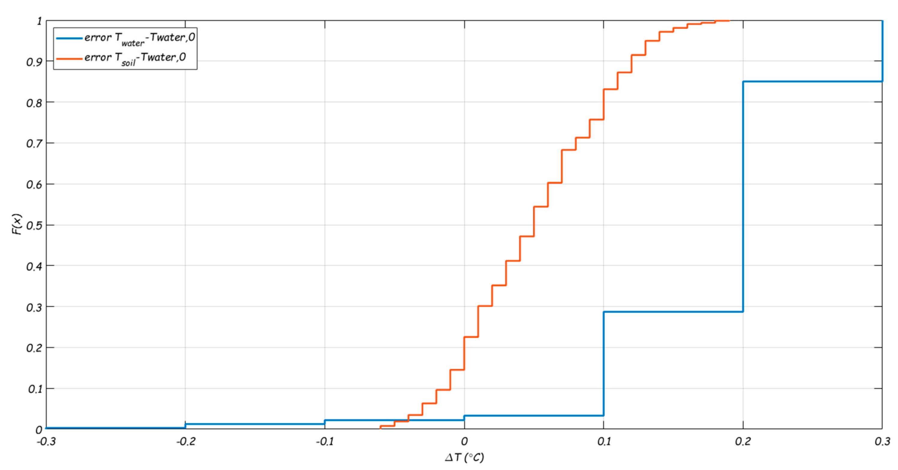
After the 9 tests were done, the sensors were calibrated in the lab. The calibration consisted of two days measuring the same water at a temperature between 16.5 and 18.5 °C. Figure B2 shows the error between the two sensors measuring Twater at L1 and L2 (error Twater – Twater, 0) and between the sensors measuring Twater at L1 and Tsoil (error Twater - Tsoil). It can be seen that Twater at L1 was usually lower than what the soil temperature sensors and the sensor Twater at L2 measured.
Figure B2.
Cumulative frequency distribution of the difference between temperature sensors during calibration.
Figure B2.
Cumulative frequency distribution of the difference between temperature sensors during calibration.
The values that were used in the WTM+ for case study 1 are listed in Table B2.
Table B2.
Parameters values of Eq. (2) and (4) for case study 1. Constants for water are used ( , , = 0.57 Wm-1K-1, = 0.14 m2s-1) .
Table B2.
Parameters values of Eq. (2) and (4) for case study 1. Constants for water are used ( , , = 0.57 Wm-1K-1, = 0.14 m2s-1) .
| Parameter | Unit | Value | Uncertainty | Reference |
|---|---|---|---|---|
| D1 | mm | 152 | - | Information from water utility Evides |
| D2 | mm | 160 | - | |
| Nu | - | Table B1 | Unclear beforehand where transition between turbulent and laminar flow is found | For turbulent flows: Nu = 0.027 Re0.8 Pr0.33 For laminar flows: Nu = 3.66 [2] |
| λpipe | Wm-1K-1 | 0.16 | - | PVC [2] |
| D3 | mm | D2 + TSoI × D1 | To be determined | |
| λsoil | Wm-1K-1 | 1.6 | +/- 0.3 °C | Measured [15] |
| Twater,0 | °C | Time series, Figure 3. | +/- 0.1 °C | Measured (L1) |
| Twater | °C | +/- 0.1 °C | Measured (L3) | |
| Tboundary | °C | +/- 0.1 °C | For flowing water, from STM+ |
B.2 Measurement Data Processing
To validate the WMT+ with these measurements we need to consider that none of the parameters in Eq. (4) are constant over time. It is required to do some data processing in order to match measurements at the beginning and end of the pipe, and to ensure that the data can be compared over time.
The normalized temperature difference (Eq. (4)) is calculated for every (15 min) datapoint (Table B3). The parameters are determined as follows:
- : The residence time follows from the measured flows.
- : drinking water temperature measured at location L1.
- : drinking water temperature measured at location L3, corrected for residence time τ (). For example, for test 4, Q = 1.4 m3/h and thus τ = 5 (L1 to L2) + 7 h (L2 to L3). Therefore, at L3, where the data during the transition time of 12 hours are discarded. Table B3 shows the residence times, and the amount of datapoints left for the analysis after discarding the transition period (see also Figure B3).
- : Tboundary was estimated with the STM+ results for L3. We thus assume that the same boundary condition is valid for the entire pipe length between L1 and L3. For the tests we assume that during the residence time the Tboundary that is experienced by the flowing water is the average of the modelled soil temperature during this residence time: , (see also Figure B3). Note that Tboundary for flowing water was used, for turbulent and laminar flows. In Figure B5 the test results with Tboundary for stagnant water are shown.
Figure B3.
Parameters for Eq. (4), after adjustment for residence time and selection of laminar and turbulent flows (Re > 5000) in the active mode and the passive mode (where no distinction in flow regime is made).
Figure B3.
Parameters for Eq. (4), after adjustment for residence time and selection of laminar and turbulent flows (Re > 5000) in the active mode and the passive mode (where no distinction in flow regime is made).
With respect to the uncertainties (εw in Twater, εs in Tboundary), it is noted that:
- : the accuracy can be estimated as . The accuracy of the flow meter is 0.004 m3/h (1 litre with a log frequency of 15 minutes). During the test phases the flow is kept more or less constant, the accuracy plus variability lead to a ΔQ equal to 0.012 m3/h. For the flow rates of Table B1 this results into less than 1 minute for the short residence times of test 5 and 6 (τ = 1 and 2 hours respectively) and almost 30 minutes for the longest residence time of test 3 (τ = 24 h). This means an uncertainty in the residence time of less than 2% and therefor is neglected.
- : the accuracy is related to the accuracy of the drinking water temperature measurements. The accuracy in and is ± 0.1 °C. The calibration that was done after the measurement period showed an average error between the two sensors at L1 and L3 (i.e. and ) of 0.2 °C (2 × εw = 0.2 °C, Figure B2). The uncertainty for the modelled is estimated as 0.1 °C [15]. When these errors have the opposite sign, the largest error will occur. With εw = −εs = 0.1 °C, the uncertainty in is determined as (see 0) . This means that when () is small, the uncertainty in is large. This uncertainty is not negligible. Figure B4 shows 985 datapoints with their corresponding normalized temperature difference ( and uncertainty bars).
The vast majority of the datapoints showed a decrease in the measured drinking water temperature (). For 22 of 985 datapoints (indicated with black error bars in Figure B4) the situation was reversed, with a decrease of 0.1°C (15 datapoints) and 0.2°C (7 datapoints). This is remarkable because the soil temperature was always lower than , which means that the drinking water temperature increased along the pipe length although the soil was cooler. Two potential explanations are considered:
- The drinking water temperature did not actually increase, but there is a measurement error. The measurement uncertainty (0.2 °C) is large compared to the measured temperature differences (0.1-0.2 °C). As so few datapoints show this effect, this explanation seems likely, and it demonstrates that measurement uncertainty needs to be considered.
- The soil temperatures were actually higher at these points, indicating that the modelled is incorrect (Table B5 shows a sensitivity to ). However, as these points were clustered in time, this explanation seems unlikely.
Figure B4 shows that the uncertainty for some measurements is quite large, especially for the tests at very short residence times (tests for 1 and 2 hours); the uncertainty appears to be smaller at higher residence times. Two explanations are considered:
- 3.
- This is a coincidence. The size of the uncertainty in ΔTN correlates with the driving force (.) and is expected to be independent of the residence time τ. It seems likely that it is just a coincidence that the driving force was relatively small during the tests with small residence times. Before the controlled residence times tests started, and data was already recorded, there were some days where ), while and the temperature of the drinking water at the PS were different.
- 4.
- There is in fact a correlation between τ and . The soil temperatures that we considered as may not be correct for all test conditions, i.e. the boundary condition cannot be retrieved from the STM+. The high flow tests (short residence times) lasted relatively short (5 to 10 hours) and the assumption of a (dynamic) equilibrium may not be valid, where it may be valid for the longer tests (at lower flows).
Figure B4.
ΔTN versus residence time, individual datapoints with corresponding uncertainty bars. Colours indicated the size of the driving force (DF = Tboundary-T(water,0)), in black negative DF, the size of uncertainty bars is equal to 0.2/DF. N.B. Tests ID2, 4, and 7 are done at 12 hours, but for readability are plotted around 12 hours.
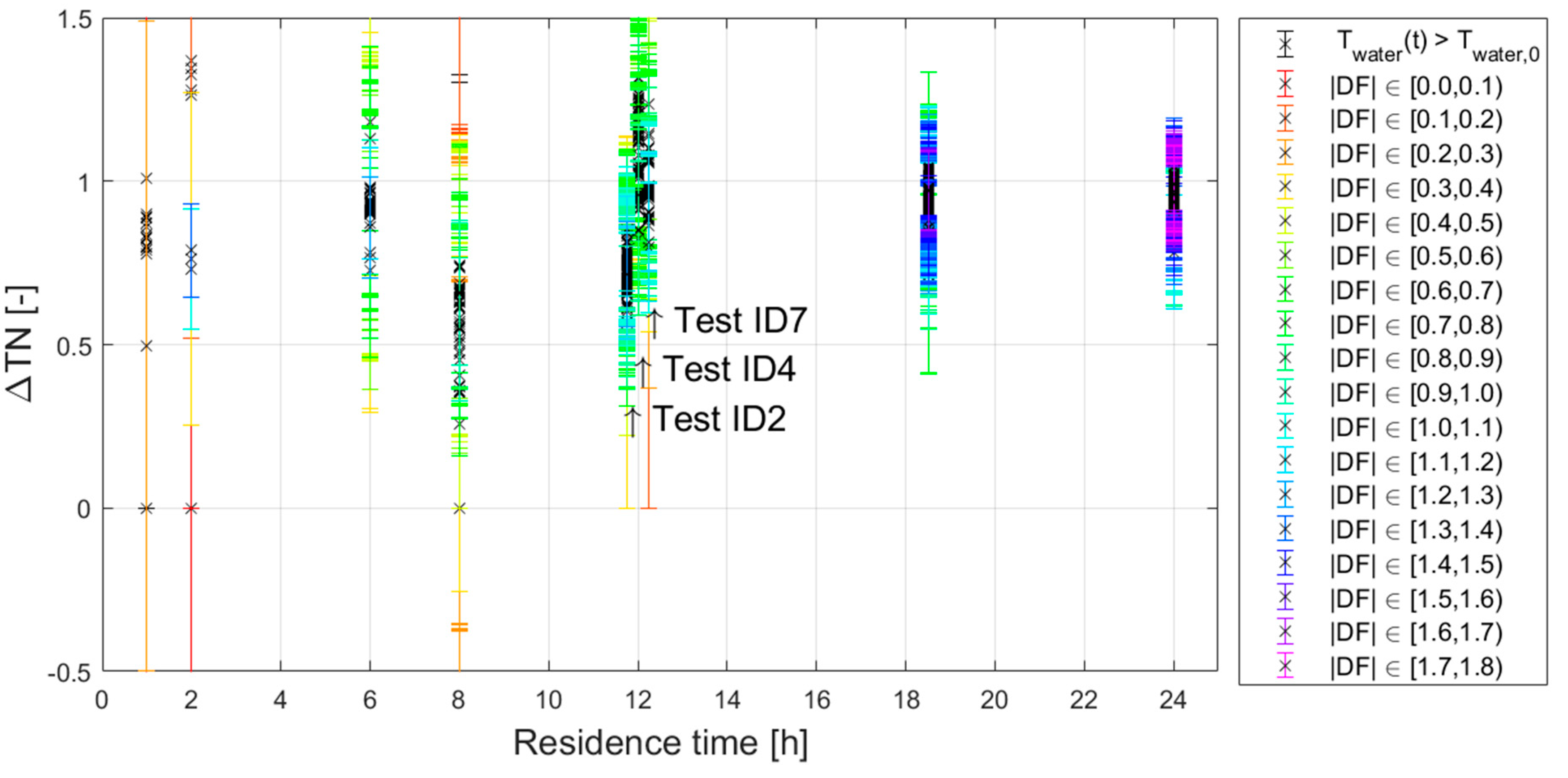
Some data was filtered out:
- The 22 datapoints with a negative driving force are excluded from the validation.
- is expected to be between 0 and 1. A datapoint with an uncertainty of > 0.5 is considered unreliable. These are datapoints for which the difference between Twater, 0 and Tboundary are small and therefor the value of ΔTN loses its meaning. There are 93 datapoints with > 0.5 (indicated with red and yellow error bars in Figure B4). These are excluded from the validation.
Figure B4 shows that some datapoints are larger than 1, and some of the datapoints including the uncertainty is smaller than 0. This should not be possible if the concept of the WTM+ is correct. It can be explained if the measured temperature differences are not correct. For this reason, the filtering step makes sense. Another explanation would be that the temperature difference between Twater, 0 and Tboundary are incorrect. Which could be caused be measurement uncertainties (basically covered by the filtering step) or model uncertainties, i.e. Tboundary is incorrect. Note that the timing of the (shift in) Tboundary may lead to an error. For test 3 e.g., the residence time between L1 and L3 is 24 hours, and the Tboundary that is being applied is the one at 12 hours from L1. In this particular case, the first 12 hours Tboundary will be an overestimate of the real boundary conditions, and the last 12 hours will be an underestimate.
As a last step, the individual datapoints with similar residence times were grouped and shown in boxplots. The measurements at residence times of 1 and 2 hours (tests 5 and 6, Table B3) have only a few datapoints and even less were left after filtering datapoints with high uncertainty in . For the remaining tests it appears that the variability between datapoints is in the same order of magnitude as the uncertainty per datapoint. Therefore, in the validation, the uncertainty in will not be explicitly shown.
Table B3.
Overview of the number of data points. between brackets the number of datapoints after filtering out measurements with high uncertainty.
Table B3.
Overview of the number of data points. between brackets the number of datapoints after filtering out measurements with high uncertainty.
| ID | Start time | End time | Residence time [h] | Amount of datapoints after adjusting for residence time (and filtering) |
|---|---|---|---|---|
| 1 | 19 May 6:30 | 20 May 16:00 | 8.0 | 103 (60) |
| 2 | 20 May 16:15 | 22 May 12:30 | 12.0 | 130 (128) |
| 3 | 22 May 13:00 | 25 May 16:30 | 24.0 | 207 (207) |
| 4 | 25 May 16:45 | 27 May 08:30 | 12.0 | 112 (109) |
| 5 | 27 May 09:15 | 27 May 20:00 | 1.0 | 41 (0) |
| 6 | 28 May 08:00 | 28 May 15:00 | 2.0 | 21 (2) |
| 7 | 28 May 15:30 | 29 May 18:45 | 12.0 | 62 (57) |
| 8 | 29 May 19:00 | 02 Jun 07:45 | 18.6 | 266 (266) |
| 9 | 02 Jun 08:15 | 03 Jun 10:00 | 6.0 | 83 (41) 1 |
B.3 Sensitivity Analysis of WTM+, Applied to a Single Pipe
For a single pipe the sensitivity analysis for was done analytically. The parameters in Eq. (2) are kept constant; one by one the parameters were multiplied with a factor of 2 or 1/2, and the effect on and the time it takes before = 0.999 were calculated. For example, halving D1, means that ΔTN increases from 0.52 to 0.84 (multiplication factor of 1.63), and the time to reach = 0.999 decreases from 23.7 to 9.4 hours (multiplication factor of 0.4). The higher the first value or the lower the second value, the more sensitive the model is towards this parameter. Table B4 shows that , and have the largest influence on and the time to reach 0.999. is not sensitive to the flow velocity in the turbulent regime (, but this is especially true for the case of a thermal insulating pipe material and D3 > D2). It should be noted that for the selected pipe diameter residence time is only important if it is less than 24 hours, which includes both laminar and turbulent flow regimes. To the other parameters is sensitive to a limited degree.
Table B4.
Sensitivity analysis with factor 2 variation in parameter values ( , , = 0.57 Wm-1K-1), evaluated at τ = 2.5 h, ≈ 0.5. Table is sorted by 5th column.
Table B4.
Sensitivity analysis with factor 2 variation in parameter values ( , , = 0.57 Wm-1K-1), evaluated at τ = 2.5 h, ≈ 0.5. Table is sorted by 5th column.
| Parameter | [unit] | Default value |
Multiplication factor |
Resulting multiplication |
Resulting multiplication factor for τ = 0.999 |
|---|---|---|---|---|---|
| Tboundary – Twater, 0 | [K] | 5 | 2 | 2.00 | 1.00 |
| D1 | [mm] | 152 | 0.5 | 1.63 | 0.40 |
| λsoil | [Wm-1K-1] | 1.60 | 2 | 1.62 | 0.40 |
| t | [s] | 9000 | 2 | 1.58 | - |
| TSoI × D1 | [m] | 0.152 | 0.5 | 1.35 | 0.61 |
| λpipe | [Wm-1K-1] | 0.16 | 2 | 1.18 | 0.78 |
| dpipe | [mm] | 4 | 0.5 | 1.11 | 0.86 |
| Nu | [-] | 100 | 2 | 1.01 | 0.98 |
Table B5 shows the results for the sensitivity analysis where more realistic parameter variations are considered. For example, when flows and residence times are not known exactly, when a mistake is made in pipe diameter, pipe wall thickness or pipe material, or another soil type is present. In (the Dutch) practice , and are typically well known. It shows that is an important parameter. In this table TSoI is not shown, this parameter is the unknown that we hope to estimate from the measurements. This shows that is not sensitive to the flow velocity in the turbulent regime (), but there is a big influence from turbulent to laminar flows.
Table B5.
Sensitivity analysis with realistic uncertainty in parameter values ( , , = 0.57 Wm-1K-1), evaluated at τ = 2.5 h, ≈ 0.5. Table is sorted by 5th column.
Table B5.
Sensitivity analysis with realistic uncertainty in parameter values ( , , = 0.57 Wm-1K-1), evaluated at τ = 2.5 h, ≈ 0.5. Table is sorted by 5th column.
| Parameter | [unit] | Default value | Realistic alternative |
Explanation | Resulting multiplication factor for τ at which = 0.999 |
|
|---|---|---|---|---|---|---|
| Nu | [-] | 100 | 3.66 | laminar flow (i.so. turbulent) | 0.61 (1/.0.61 = 1.64) |
1.90 (1/1.90 = 0.52) |
| 400 | Q: 0.1 to 0.7 m/s | 1.02 | 0.97 | |||
| λsoil | [Wm-1K-1] | 1.60 | 1.9 | wet sand (i.so. dry sand) | 1.34 | 0.62 |
| D1 | [mm] | 152 | 125 | one step down in nominal diameter | 1.18 | 0.77 |
| λpipe | [Wm-1K-1] | 0.16 | 0.4 | PE (i.s.o. PVC) | 1.18 | 0.78 |
| dpipe | [mm] | 4 | 3 | one step down in pressure class | 1.05 | 0.93 |
| t | [s] | 9,000 | 10,000 | measurement inaccuracy (ca. 15 minutes) | 1.12 | - |
| Tboundary – Twater, 0 | [K] | 5 | 4.8 | measurement inaccuracy (0.2 K) | 1.04 | 1.00 |
B.4 Extra Results for Case Study 1
Figure B4 shows ΔTN versus residence time with the measurement in boxplots and theoretical lines for various values of TSoI, for the case where Tboundary was taken from the STM+ passive mode.
Figure B5.
Figure B5.
ΔTN versus residence time, with Tboundary from STM+ passive model. Measure data are shown in boxplots. The curves represent Eq. (4) with different values for the TSoI. The threshold for turbulent flows is determined at Re = 5,000. Datapoints (22) with ΔTN < 0 are begin discarded. Datapoints (1) with E ≥ 0.5 are being discarded.
Appendix C (Case Study 2)
C.1 Additional Information on Case Study 2: Soil Temperatures
The local circumstances that influence the soil temperature around the pipes are determined by the pipe installation depth, soil type, soil cover and local anthropogenic heat sources. Specifically for the Almere DWDN the following is found:
- There is a variation in installation depth with the top of the distribution mains in the older parts (built between 1980 and 2000, roughly the centre and southern part, amongst which areas A and D in Figure 6) at -1.3 m and in the newer parts (roughly the western and north-eastern part, amongst which areas B, E and C in Figure 6) at -1.1 m (meaning that the centre of the Ø110 and Ø160 mm pipes are installed at -1.35 to -1.38m, respectively -1.15 to -1.18 m). The transport mains (> 180 mm) are installed at ca. 1.5 m coverage (centre of the Ø200 and Ø310 mm pipe at ca. -1.6 to -1.7 m).
- The soil type is influenced by the backfill that was used for pipe installation. The older parts have a mixture of sand and clay, and the newer parts have sand only.
- The variation in soil cover (asphalt, tiles, grass, or bushes) is very high, and very distributed over the entire area. There even is soil cover variation over the length of a single pipe. This level of detail was not considered in this study.
- Above ground anthropogenic heat sources were not considered either. It is not yet entirely clear which are important and how much influence they would have.
- Below ground anthropogenic heat sources include electricity cables and DHN, where the DHN most likely has a significant effect [15]. The northwestern part of Almere (amongst which areas A and C in see Figure 6) has a DHN. The effect of the DHN parallel to the DWN is not considered in this paper as the distance between the two is more than 2.5 m. The crossings of DWDN and DHN pipes are taken into consideration.
The areas with pipes at -1.35 m and with a clay and sand mixture backfill roughly overlap; and the areas with pipes at -1.15 m and with a sand backfill also roughly overlap. This means that there are transport mains with and without DHN crossings, distribution mains in the older parts of the network with and without DHN crossings and distribution mains in the newer parts of the network (only without DHN crossings).
For these five subgroups of pipes a specific value of Tboundary was determined for 31 August 2020. The parameters of Eq. (1) are determined as follows:
- : The residence time follows from the hydraulic network model. Here, the demand patterns of 31 August 2020 were applied, but the model was not calibrated for this particular day, so there may be some valve positions that are incorrect which may lead to errors in residence time.
-
: was estimated by using weather data, processed with the STM [2,16] and STM+ [15]. There were no soil temperature measurements available. Five different boundary conditions were suggested (Table C2):
- TTM is the soil temperature around transport mains (D ≥ 180 mm). TTM = 18.0 °C. This is the STM calculated temperature at -1.7 m (Figure C), in peri-urban area (clay/sand under grass);
- TTM_DHN is the soil temperature around transport mains with crossing DHN. TTM_DHN = 20.1 °C. This is the STM calculated temperature at -1.7 m, in peri-urban area (clay/sand under grass) + 2.1 °C from the primary network DHN as from the STM+;
- TTM is the soil temperature around distribution mains in the older part of Almere. TDM = 18.7 °C. This is the STM calculated temperature at -1.35 m (Figure C), in peri-urban area (clay/sand under grass);
- TTM is the soil temperature around distribution mains with crossing DHN, in the older part of Almere. TDM_DHN = 19.5 °C. This is the STM calculated temperature at -1.35 m, in peri-urban area (clay/sand under grass) + 0.8 °C from the secondary network DHN as from the STM+;
- TTM_NE is the soil temperature around distribution mains in the newer (north-eastern) part of Almere. TDM_NE = 20.5 °C. This is the maximum drinking water temperature that was measured in area B (Figure 6), and is the average of the STM calculated temperatures at -1.15 m (Figure C) for peri-urban (clay/sand under grass) and urban (sand, under tiles with various shade conditions).
- : drinking water temperature measured at locations F1 and F2 (13.7 and 13.3 °C respectively).
- : drinking water temperature measured at hydrants (Figure 6)
Figure C1.
Modelled soil temperature (STM) at various depths for 31 August 2020. Indicated are temperatures around transport mains (TTM:), transport mains with crossing of DHN (TTM DHN), distribution mains in most of Almere (TDM), distribution mains with crossing of DHN (TDM DHN), distribution mains in area B (TDM B).
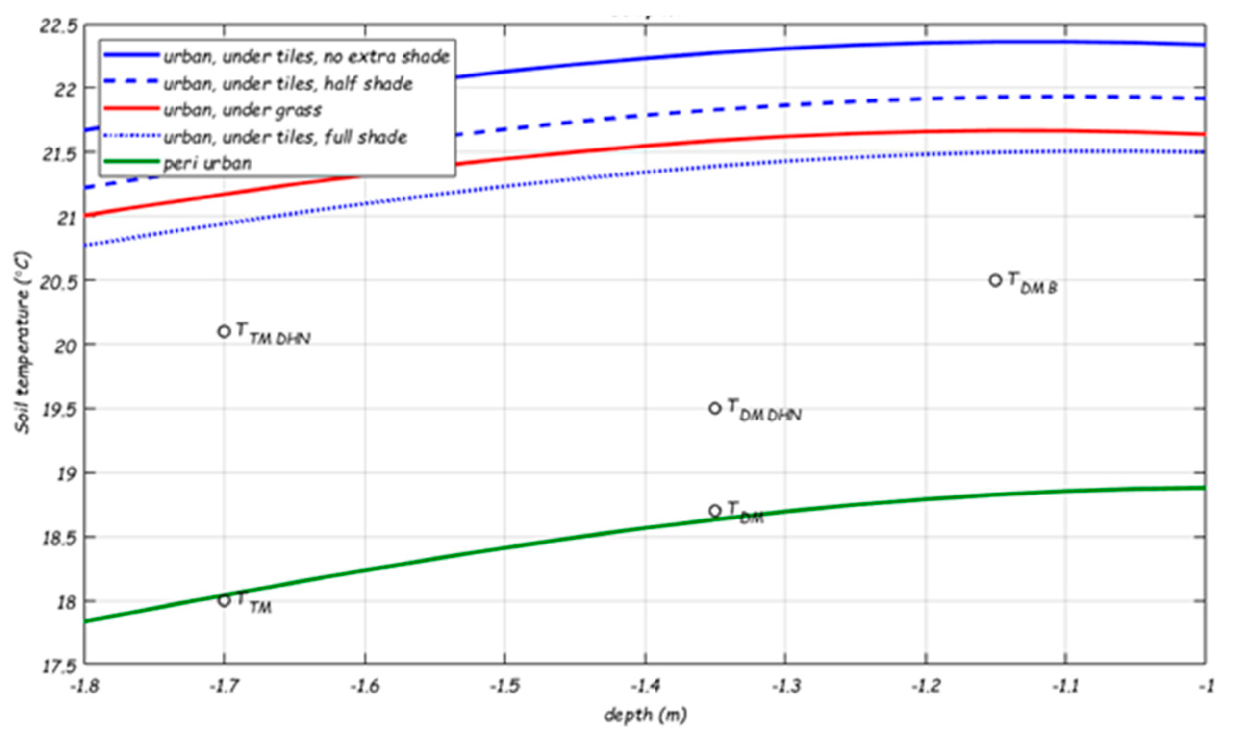
Table C1.
Settings of STM [3] where weather input data were used from Schiphol airport (20 km from Almere).
Table C1.
Settings of STM [3] where weather input data were used from Schiphol airport (20 km from Almere).
| Scenario | λsoil | ρsoil | Cp, soil | αsoil | Cover | albedo | Global radiation |
QF | a3 |
|---|---|---|---|---|---|---|---|---|---|
| W.m.K-1 | kg.m−3 | J.kg-1.K-1 | 10-6 m2s-1 | - | W.m-2 | W.m-2 | W.m-2 | ||
| Peri-urban, under grass (clay) |
1.0 | 2.103 | 1.103 | 0.5 | Grass | 0.12 | Rg | 50 | -50 |
| Urban, under grass (sand) |
1.2 | 2.103 | 1.103 | 0.6 | Grass | 0.12 | Rg | 100 | -100 |
| Urban, under tiles, no extra shade (sand) |
1.2 | 2.103 | 1.103 | 0.6 | Tiles | 0.12 | Rg | 100 | -100 |
| Urban, under tiles, half shade (sand) |
50% × Rg | ||||||||
| Urban, under tiles, full shade (sand) |
0 |
Table C2.
Tboundary for Almere network model.
| Tboundary | value | Pipe group conditions | Where in network | Where in model |
|---|---|---|---|---|
| TTM | 18.0 °C. | -1.5 m, sand + clay, no DHN crossings |
Most transport mains (> 180 mm) | |
| TTM_DHN | TTM + 2.1 = 20.1 °C. | -1.5 m, sand + clay, with DHN crossings |
Some transport mains (> 180 mm) with crossings of DHN | |
| TDM | 18.7 °C. | -1.3 m, sand + clay, no DHN crossings |
Area A and D | distribution mains in whole network, except area B |
| TDM_DHN | TDM + 0.8 = 19.5 °C. | -1.3 m, sand + clay, with DHN crossings |
Part of Area A with crossings of DHN | distribution mains in whole network, except area B |
| TDM_NE | 20.5 °C. | -1.1 m, sand, no DHN crossings |
Area B, C and E | distribution mains in area B |
C.2 Additional Information on Case Study 2: WTM+
The hydraulic model of the area (provided by Vitens) is characterized by 21054 nodes and 21987 pipes. To simulate the drinking water temperature in this network, the WTM+ (Eqs. (1) and (2)) was integrated into an Epanet-MSX model. Epanet-MSX requires some general settings (a 5th order Runge-Kutta integrator was used as solver, the hydraulic model was used to evaluate 72 hours, results are saved and analysed for the last 24 hours) and case specific settings (Table C3).
Table C3.
Parameters values of Eq. (2) and (4) for case 2. Constants for water are used ( , , = 0.57 Wm-1K-1, = 0.14 m2s-1).
Table C3.
Parameters values of Eq. (2) and (4) for case 2. Constants for water are used ( , , = 0.57 Wm-1K-1, = 0.14 m2s-1).
| Parameter | Unit | Value | Uncertainty | Reference |
|---|---|---|---|---|
| D1 | mm | 50-300 | - | Hydraulic network model Almere, from Vitens |
| D2 | mm | 1.052 × D1 | - | Outside diameter of PVC estimated with multiplication factor to inside diameter. AC pipes treated as PVC. |
| λpipe | Wm-1K-1 | 0.16 | Some pipes are AC, but modelled as PVC | AC pipes treated as PVC [2] |
| Nu | - | Unclear where transition between turbulent and laminar flow is, transition at Re = 5,000 from case study 1 | For Re > 5,000:Nu = 0.027 Re0.8 Pr0.33 [2], Re from Hydraulic network model Almere, Pr = 7. For Re <= 5,000 Nu = 3.66 |
|
| D3 | mm | D2 + TSoI × D1 | ? | To be determined |
| λsoil | Wm-1K-1 | 1.6 | Unknown | dry sand [15] |
| Twater,0 | °C |
= 13.7 =13.3 |
+/- 0.05 °C | Vitens |
| Twater | °C | 13.0-21.0 | +/- 0.05 °C | Measured at hydrants, Vitens |
| Tboundary | °C | TDM = 18.7 TDM_DHN = 19.5 TDM_NE = 20.5 TTM = 18TTM_DHN = 20.1 |
? | For stagnant water, from STM (Table C2). |
C.3 Sensitivity Analysis of WTM+, Applied to a Drinking Water Distribution Network
The sensitivity analysis of the single pipe is insightful. However, in a network with a variety of pipe diameters and topologies, residence times in the different types of pipes (e.g. transport and distribution mains of different lengths) will vary. Executing an effective sensitivity study of the drinking water temperature at household connections in a DWDN is not straightforward. Therefore, a limited sensitivity analysis is done for case study 2 where we only focus on the most important parameters, as they follow from the previous section, namely TSoI, , . Pipe length and pipe diameter were added.
Five areas (A-E) were selected for the sensitivity analysis. The areas differ in surrounding soil temperatures and residence times from the sources. Area A and B are comparable in residence time from the sources (Table C4). Area C is far from the reservoir, with a large residence time. Area D is the oldest neighbourhood (built in the 1980s) and has an older design philosophy (larger diameters, more looped than area A and B). Area E is very close to the reservoir (see Figure 6). A DHN is installed next to the DWDN in areas A and C, but not in areas B, D and E.
Table C4.
Residence times of study areas in Almere DWDN.
| Residence time (h) | Conditions for Tboundary | ||
|---|---|---|---|
| A | 13.3 | 5-15 | TDM, TDM_DHN |
| B | 13.7 | 10-15 | TDM_NE |
| C | 13.3 | > 24 | TDM, TDM_DHN |
| D | 13.3 | > 10 | TDM |
| E | 13.7 | 10-15 | TDM_NE |
The parameter values for the base case are best guesses from a priori knowledge of the area, see Section 0. This case serves as a reference for the sensitivity analysis. In the sensitivity analysis, the TSoI was varied between 0.1 and 10. To test the sensitivity to the soil temperature was specified in various scenarios for the five subgroups of pipes (i.e. transport mains with and without DHN crossings, distribution mains with and without DHN crossings and distribution mains in the north-east without DHN crossings). For a range from 1.1 to 1.9 was used. To test the effect of street lengths, the pipe length was increased and decreased by 10%; to test the effect of different design philosophies, the pipe diameter was increased and decreased by 10% (Table C5). Furthermore, the areas A-E were analysed separately to identify the effect of network layout and residence time from the reservoirs.
Table C5.
Settings for scenarios for sensitivity analysis. Blanks are equal to the base case. Other parameter values are in Table C3.
Table C5.
Settings for scenarios for sensitivity analysis. Blanks are equal to the base case. Other parameter values are in Table C3.
| Scenario | Scale% | TSoI | TDM °C |
TDM_DHN °C |
TDM_NE °C |
TTM °C |
TTM_DHN °C |
|
|---|---|---|---|---|---|---|---|---|
| Base | 1 | 1.6 | 18.7 | 19.5 | 20.5 | 18.0 | 20.1 | |
| TSoI | 0.1-10 | |||||||
| 14.7-23.1 | TDM+0.8 | TDM – 0.5 | TDM+1.4 | |||||
| 15.0-23.0 | ||||||||
| 13.7-24.2 | ||||||||
| 13.7-24.2 | ||||||||
| 13-23 | ||||||||
| λsoil | 1.1-1.9 | |||||||
| D1 | -10 to +10 | |||||||
| Pipe length | -10 to +10 |
For all scenario’s, the drinking water temperature (Twater) was determined at all time steps (t) at all non-zero demand nodes (n). All scenario results were compared to the base case (Table C3, Table C5), i.e. the temperature difference (ΔT(t,n) = Twater, base (t, n) - Twater, scenario (t,n)) was calculated. Next the average of ΔT over all time steps and all nodes was calculated for each area (A-E) separately, plus for the total network. Note that ΔT can be negative or positive.
The sensitivity analysis shows the following:
- TSoI: Figure C2a shows that ΔT ≤ 0.8 °C for a TSoI < 1. The larger the TSoI, the slower the heat exchange between soil and drinking water, and in this case it means that at larger TSoI, Twater,(t, n) will be lower. Figure C2a shows that the effect is similar for most areas, but stronger in area B. This is most likely caused by a difference in residence times. The residence times towards area C e.g. are large (> 20 h) and thus most likely the drinking water temperature at most nodes has reached Tboundary, even with an extra delay due to the TSoI, leading to a maximum of ΔT = 0.8 °C. On the other hand, areas B and E are very close to a reservoir, and the effect of a larger TSoI is more noticeable (ΔT ≥ 1.2 °C).
-
Tboundary: The model is very sensitive to Tboundary. Especially scenario shows a large effect; the other scenarios have a are more local effect, and the effect is smaller (Figure C2b). The larger the area where this local Tboundary is imposed, the larger the number of customers nodes that are affected.
- The scenario shows that when Tboundary decreases or increases at (almost) all locations (Figure C2c), the Twater,(t, n) changes with it. The effect is small (but not zero) in areas B and E, where Tboundary is the same as in the base case.
- The scenario shows the local effect of TDM_NE only in the areas that have this boundary condition (Area B and E), there is no effect in areas A, C and D. A range of 8 °C (from 15 to 23 °C) in TDM_NE leads to a range of 5 °C (-2.5 to 1.5 °C) in ΔT and thus in Twater,(t, n) in areas B and E (Figure C2d).
- The scenario (Figure C2e) shows the effect when only Tboundary around transport mains are changed. A 8 °C change in Tboundary leads to ca. 1.5 °C change in Twater,(t, n).
- The scenario (Figure C2f) shows that a different Tboundary at DHN crossings with the distribution mains has a small effect, but larger than 0 °C. This effect is more apparent when we only look at the areas that have distribution mains with DHN crossings (areas A and C), where the effect is larger in area C (a 8 °C change in Tboundary leads to ca. 5 °C change in Twater,(t, n)) with longer residence times than in area A. Also in area A the effect is noticeable, and should not be neglected.
- The scenario, Figure C2b) only considers the crossings of DHN with transport mains. The effect is almost 0 (< ± 0.2 °C). This means that the current number of DHN crossings with the transport mains do not lead to higher Twater,(t, n).
- : the ΔT due to variations in is less than ± 0.3 °C (Figure C2g) and this means that is not the most important parameter to estimate accurately for the WTM+ in a real DWDN. It should be noted that Tboundary, as estimated with the STM, is indeed sensitive to .
- Pipe length and diameter: the ΔT is less than ± 0.15 °C for pipe length and diameter changes (Figure C2h); the WTM+ is not very sensitive to these parameters. This means that when the WTM+ is applied to the DWDN of case study two the results will be representative for a range of DWDN throughout the Netherlands and the five areas are representative for the effects of differences in residence time, local Tboundary and network layouts.
Figure C2.
Sensitivity analysis results. In each figure, curves A to E give the average (across all nodes and timesteps in a separate area of the network A to E) difference in modelled temperatures (compared to the modelled temperature of base scenario) due to a variation in: (a) TSoI (b-f) (f) (g) Pipe length and diameter.
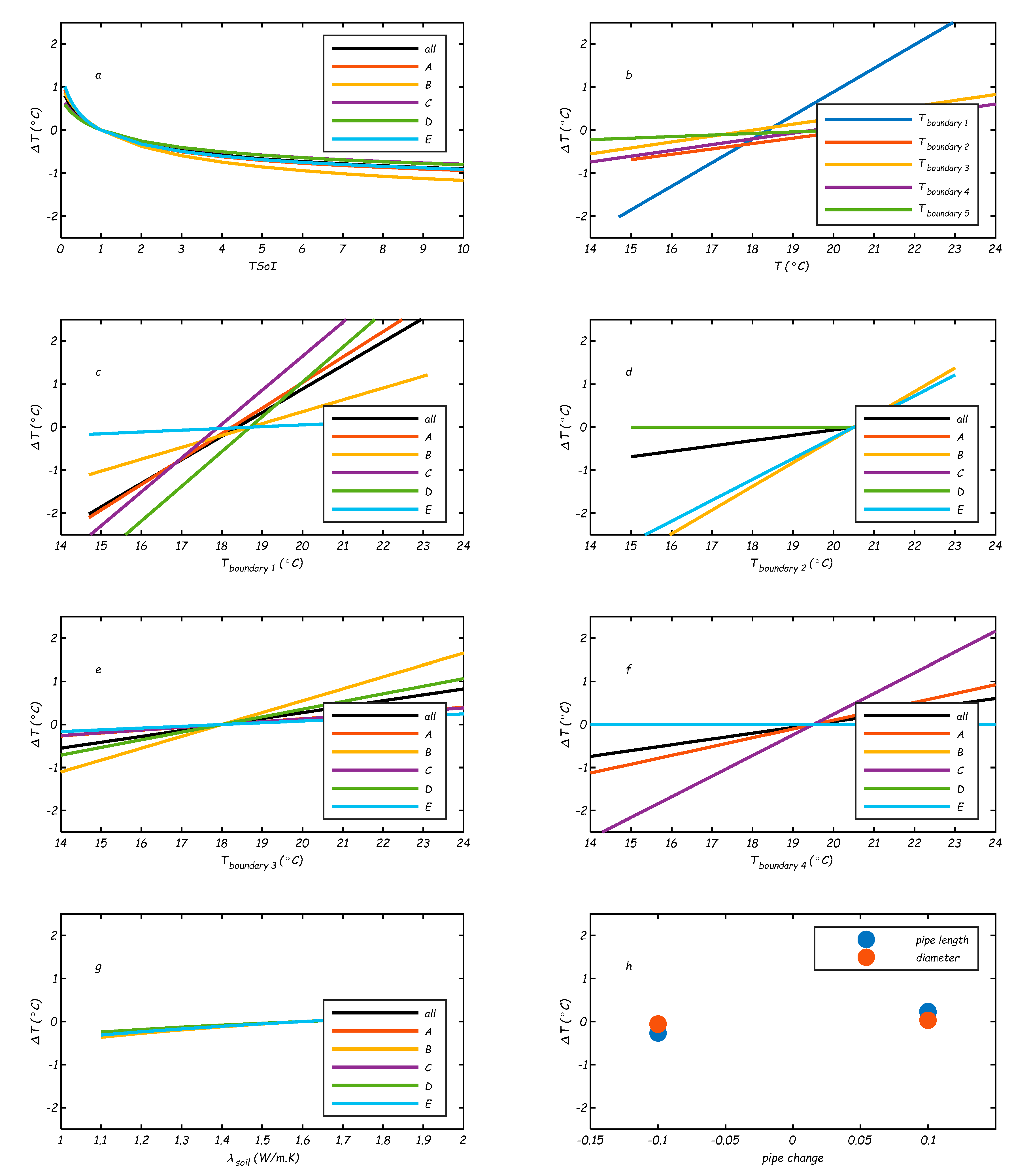
C.4 Extra Results for Case Study 2
For the extra cases, the TSoI was varied between 0.1 and 1 in steps of 0.1, and between 1 and 10 in steps of 1, meaning 19 different TSoI values were simulated. Tboundary was varied for area A (resp. area B) between 18.0-21.0 °C (19.0-22.0 °C) in steps of 0.1 °C, meaning 30 different Tboundary values were considered for both areas A and B separately. The combination of the two would mean 19 × 30 × 30 = 17100 simulations. To save simulation time, 19 simulations were run for a specific Tboundary and varying TSoI. Then the resulting at the measurement locations were converted to for the varying Tboundary values by substituting them into Eq. (3).
With for area (resp. area B) = 13.7 °C (13.3 °C) and = 20.5 °C (19.5 °C), and = 18.0-21.0 °C (19.0-22.0 °C). Note that in Eq. (C1) the boundary conditions are not time dependent as they are in case study 1. This approach calculates the value for τ from the modelled temperatures, instead of using them directly from the hydraulic network model. Note that the results are not as accurate as a new simulation would be, as was assumed to be a single value, instead of changing between pumping station and measurement location, with a variable residence time in pipes with different diameters.
Compared to the base case, a larger TSoI (> 1) will lead to a slower change of the drinking water temperature. There will be locations where Twater will not yet have reached Tboundary, which will result in a lower Twater than at TSoI = 1. There will also be locations that have relatively high residence times and Twater will have reached Tboundary, which means that Twater will be the same as in the base case. A larger Tboundary will lead to an increase in all modelled drinking water temperatures, with the largest effect in absolute terms at the locations with higher residence times. This means that a change in TSoI mostly affects the temperatures at lower residence times, and a change in Tboundary mostly affects the temperatures at higher residence times. When both parameters are changed simultaneously, the parameter leadings to the smallest error with respect to the measurements can be found. Figure C3a illustrates the effect for changing TSOI compared to the base case. It shows that most cyan points (TSoI = 2) are lower than the magenta points (TSoI = 1), and the difference is much smaller near Tmodelled = 20.5 °C (which is the maximum), then e.g. at Tmodelled = 17 °C. Figure C3b illustrates the effect for changing Tboundary compared to the base case. It shows that lowering Tboundary (cyan points experience a Tboundary = 0.5 °C lower than the magenta points) leads to lower temperatures for all locations, but most distinctively for the locations with higher temperatures.
Figure C3.
Validation of WTM+, model results compared to field measurements for (left) the base case (Tboundary = 19.5 and 20.5 °C for area A and area B respectively) at TSoI = 1 and TSoI = 2, and (right) the extra case with adjusted Tboundary = 18.5 and 19.5 °C for area A and area B respectively.
Figure C3.
Validation of WTM+, model results compared to field measurements for (left) the base case (Tboundary = 19.5 and 20.5 °C for area A and area B respectively) at TSoI = 1 and TSoI = 2, and (right) the extra case with adjusted Tboundary = 18.5 and 19.5 °C for area A and area B respectively.
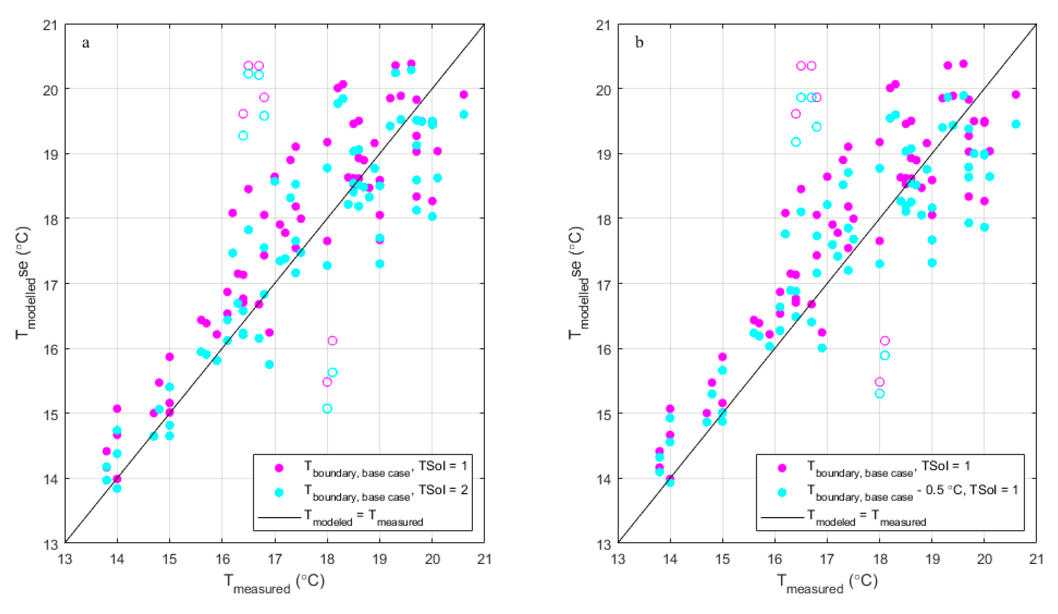
Figure C4 shows the RMSE and R2 as a function of the TSoI for Tboundary as in the base case (this is the same as the TSoI scenario in Section 0). The RMSE decreases from 1.5 °C (without outliers) to 0.76 °C with an increase of the TSoI from 0.05 to 2; and then increases again for TSoI > 2. At the same time, the R2 increases from < 0 (without outliers) to 0.80, and then decreases. For the combination of areas A and B there appears to be an optimum at TSoI = 2, with the values for Tboundary as in the base case. For area A, resp. area B, by themselves there appears to be an optimum at TSoI = 1, resp. TSoI = 3, with the base case values for Tboundary. The same exercise has been repeated with adjusted for the extra cases. The goodness of fit parameters are given in Table C6.
Figure C4.
RMSE (left) and R2 (right) for the modelled data compared to the measured data for various values of TSoI, for all measurements, including (red dotted line) and excluding outliers (red full line), and the areas A (green) and B (blue) without the outliers.
Figure C4.
RMSE (left) and R2 (right) for the modelled data compared to the measured data for various values of TSoI, for all measurements, including (red dotted line) and excluding outliers (red full line), and the areas A (green) and B (blue) without the outliers.
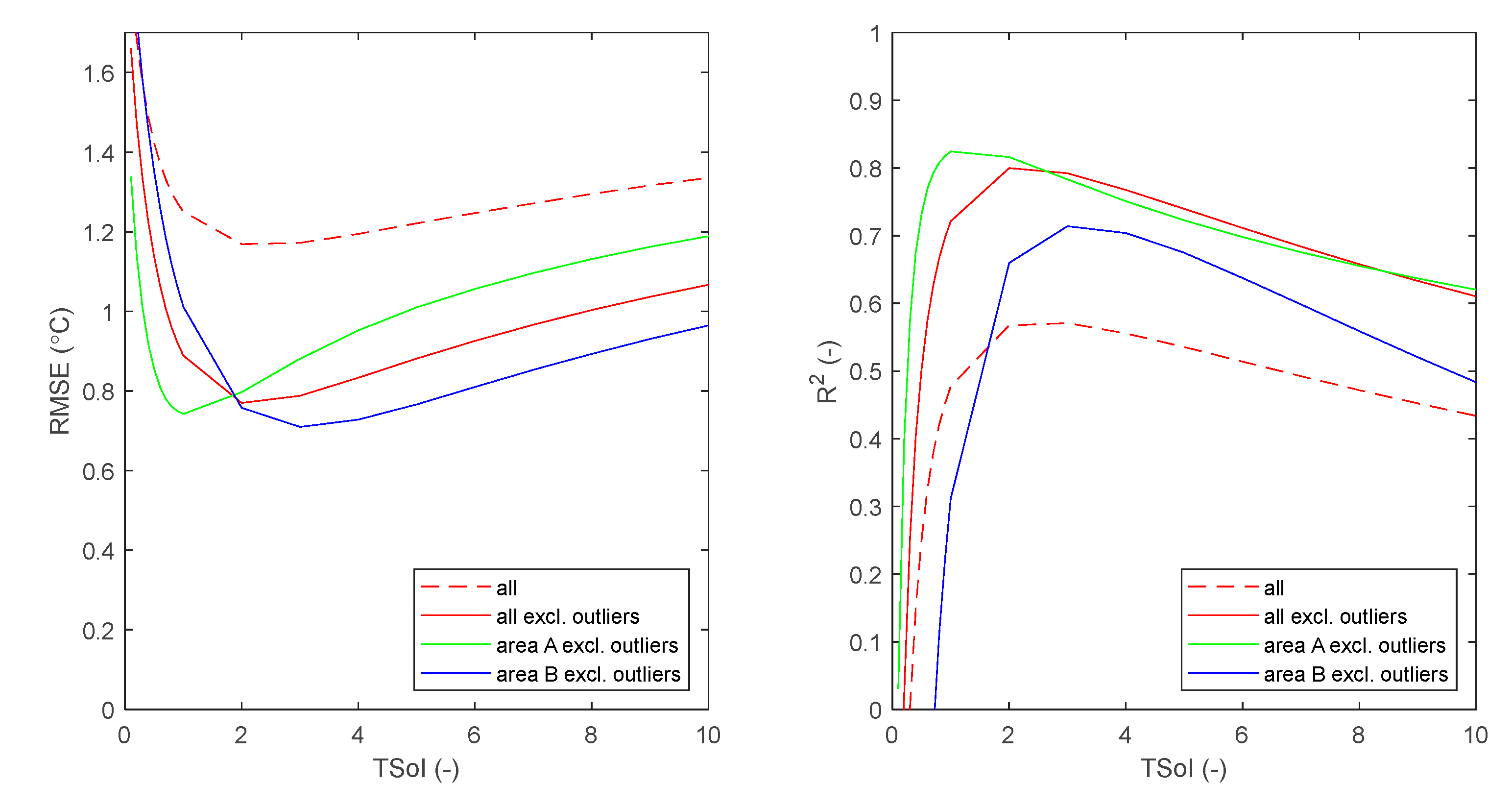
Table C6.
Goodness of fit parameters for the base case, best fit base case (best TSoI) and best fit extra cases (combination of best fit TSoI and Tboundary).
Table C6.
Goodness of fit parameters for the base case, best fit base case (best TSoI) and best fit extra cases (combination of best fit TSoI and Tboundary).
| Figure, line colour | Area | Case | Tboundary (°C) |
TSoI | Excluding outliers |
Including outliers |
||
|---|---|---|---|---|---|---|---|---|
| RMSE (°C) |
R2 | RMSE (°C) |
R2 | |||||
| Figure 7a , red | A | Base | 19.5 | 1 | 0.75 | 0.82 | 0.92 | 0.72 |
| Figure 7a , blue | B | Base | 20.5 | 1 | 1.01 | 0.31 | 1.49 | 0 |
| Figure C3a+b, magenta | Total | Base | 19.5 / 20.5 | 1 | 0.92 | 0.72 | 1.25 | 0.48 |
| n.a. | A | Change in TSoI | 19.5 | 2 | 0.80 | 0.82 | 1.03 | 0.68 |
| n.a. | B | Change in TSoI | 20.5 | 2 | 0.76 | 0.66 | 1.29 | 0.08 |
| Figure C3a, cyan | Total | Change in TSoI | 19.5 / 20.5 | 2 | 0.77 | 0.80 | 1.17 | 0.57 |
| n.a. | A | Change in Tboundary | 19.0 | 1 | 0.88 | 0.71 | 1.06 | 0.56 |
| n.a. | B | Change in Tboundary | 20.0 | 1 | 0.80 | 0.50 | 1.24 | 0 |
| Figure C3b, cyan | Total | Change in Tboundary | 19.0 / 20.0 | 1 | 0.83 | 0.72 | 1.15 | 0.49 |
| n.a. | A | best fit TSoI | 19.5 | 1 | 0.75 | 0.82 | 0.92 | 0.72 |
| n.a. | B | best fit TSoI | 20.5 | 3 | 0.71 | 0.71 | 1.22 | 0.21 |
| Figure C3a, cyan | Total | best fit TSoI | 19.5 / 20.5 | 2 | 0.77 | 0.80 | 1.17 | 0.57 |
| Figure 7b, red | A | Optimal, best fit (RMSE) Tboundary AND TSoI |
20.1 | 2 | 0.70 | 0.88 | ||
| n.a. | best fit (R2) Tboundary AND TSoI |
20.5 | 3 | 0.74 | 0.89 | |||
| Figure 7b, blue | B | Optimal, best fit (RMSE) Tboundary AND TSoI |
20.1 | 2 | 0.70 | 0.67 | ||
| n.a. | best fit (R2) Tboundary AND TSoI |
21.4 | 7 | 0.78 | 0.74 | |||
| n.a | Total | best fit (RMSE) Tboundary AND TSoI |
20.1 | 2 | 0.70 | 0.83 | ||
| n.a. | best fit (R2) Tboundary AND TSoI |
20.5 | 3 | 0.72 | 0.84 | |||
References
- Agudelo-Vera, C., S. Avvedimento, J. Boxall, E. Creaco, H. de Kater, A. Di Nardo, A. Djukic, I. Douterelo, K.E. Fish, P.L. Iglesias Rey, N. Jacimovic, H.E. Jacobs, Z. Kapelan, J. Martinez Solano, C. Montoya Pachongo, O. Piller, C. Quintiliani, J. Rucka, L. Tuhovcak, and M. Blokker, Drinking Water Temperature around the Globe: Understanding, Policies, Challenges and Opportunities. Water, 2020. 12(4): p. 1049. [CrossRef]
- Blokker, E.J.M. and E.J. Pieterse-Quirijns, Modeling temperature in the drinking water distribution system. Journal - American Water Works Association, 2013. 105(1): p. E19-E29. [CrossRef]
- Agudelo-Vera, C.M., M. Blokker, H. de Kater, and R. Lafort, Identifying (subsurface) anthropogenic heat sources that influence temperature in the drinking water distribution system. Drink. Water Eng. Sci., 2017. 10(2): p. 83-91. [CrossRef]
- Agudelo-Vera, C.M., E.J.M. Blokker, and E.J. Pieterse-Quirijns, Early warning system to forecast maximum temperature in drinking water distribution systems. Journal of Water Supply: Research and Technology - AQUA, 2015. 64(5): p. 496-503. [CrossRef]
- De Pasquale, A., A. Giostri, M. Romano, P. Chiesa, T. Demeco, and S. Tani, District heating by drinking water heat pump: Modelling and energy analysis of a case study in the city of Milan. Energy, 2017. 118: p. 246-263. [CrossRef]
- Hubeck-Graudal, H., J.K. Kirstein, T. Ommen, M. Rygaard, and B. Elmegaard, Drinking water supply as low-temperature source in the district heating system: A case study for the city of Copenhagen. Energy, 2020. 194: p. 116773. [CrossRef]
- Díaz, S., J. Boxall, L. Lamarche, and J. González, The impact of ground heat capacity on drinking water temperature. Journal of Water Resources Planning and Management, 2023. 149(5): p. 04023012. [CrossRef]
- Hypolite, G., J.-H. Ferrasse, O. Boutin, S. Del Sole, and J.-F. Cloarec, Dynamic modeling of water temperature and flow in large water system. Applied Thermal Engineering, 2021. 196: p. 117261. [CrossRef]
- Jakubek, D., P. Ocłoń, M. Nowak-Ocłoń, M. Sułowicz, P.S. Varbanov, and J.J. Klemeš, Mathematical modelling and model validation of the heat losses in district heating networks. Energy, 2023. 267: p. 126460. [CrossRef]
- Hussein, A. and A. Klein, Modelling and validation of district heating networks using an urban simulation platform. Applied Thermal Engineering, 2021. 187: p. 116529. [CrossRef]
- Danielewicz, J., B. Śniechowska, M. Sayegh, N. Fidorów, and H. Jouhara, Three-dimensional numerical model of heat losses from district heating network pre-insulated pipes buried in the ground. Energy, 2016. 108: p. 172-184. [CrossRef]
- Wang, H., H. Meng, and T. Zhu, New model for onsite heat loss state estimation of general district heating network with hourly measurements. Energy conversion and management, 2018. 157: p. 71-85. [CrossRef]
- Kuntuarova, S., T. Licklederer, T. Huynh, D. Zinsmeister, T. Hamacher, and V. Perić, Design and Simulation of District Heating Networks: A Review of Modeling Approaches and Tools. Energy, 2024: p. 132189. [CrossRef]
- Hägg, R., Dynamic simulation of district heating networks in Dymola. 2016.
- van Esch, J., BTM+ model and Expert tool. 2022, Delft: Deltares.
- Blokker, E.J.M. and E.J. Pieterse-Quirijns, Erratum - Blokker, E.J.M., Pieterse-Quirijns, E.J. Modeling temperature in the drinking water distribution system - JAWWA 105(2013)1, E19-E29. JAWWA, 2018. 110(10): p. 98.
- Çengel, Y.A., Heat transfer: a practical approach. 1998: McGraw-Hill Companies, Inc. 1006.
- Trinh, K.T., On the critical Reynolds number for transition from laminar to turbulent flow. arXiv preprint arXiv:1007.0810, 2010.
- Blokker, E., A. van Osch, R. Hogeveen, and C. Mudde, Thermal energy from drinking water and cost benefit analysis for an entire city. Journal of Water and Climate Change, 2013. 4(1): p. 11-16. [CrossRef]
- Shang, F. and J.G. Uber, EPANET Multi-species extension user's manual. 2008, Cincinnati, OH: EPA.
- Blokker, E.J.M., J.R.G. van Summeren, and K.A. van Laarhoven. Measuring drinking water temperature changes in a distribution network in WDSA CCWI. 2022. Valencia, Spain.
- .
Figure 1.
Schematic view of water and surrounding soil temperature versus distance R from the pipe centre, for a Ø160 mm PVC pipe. On the left (a) the old model approach with STM and WTM, where the soil has an infinite heat capacity. On the right (c) the model approach of the STM+, with a fitted WTM+, where the drinking water has an infinite heat capacity. In the middle (b) a hypothesized actual situation where soil and drinking water temperature affect each other. The red lines describe the WTM(+) for three values of Twater (15, 22.5 and 26.5 °C). The time it takes to go from one situation to the next differs in the three modelling approaches, indicated as tx, ty, tz and tx’, ty’, tz’. The green dots indicate the coupling between WTM+ and STM+ both in distance from the pipe wall (R3) and temperature value (Tboundary). The solid blue line (right) shows the STM(+) result, as taken from fig 6.10 in van Esch [15].
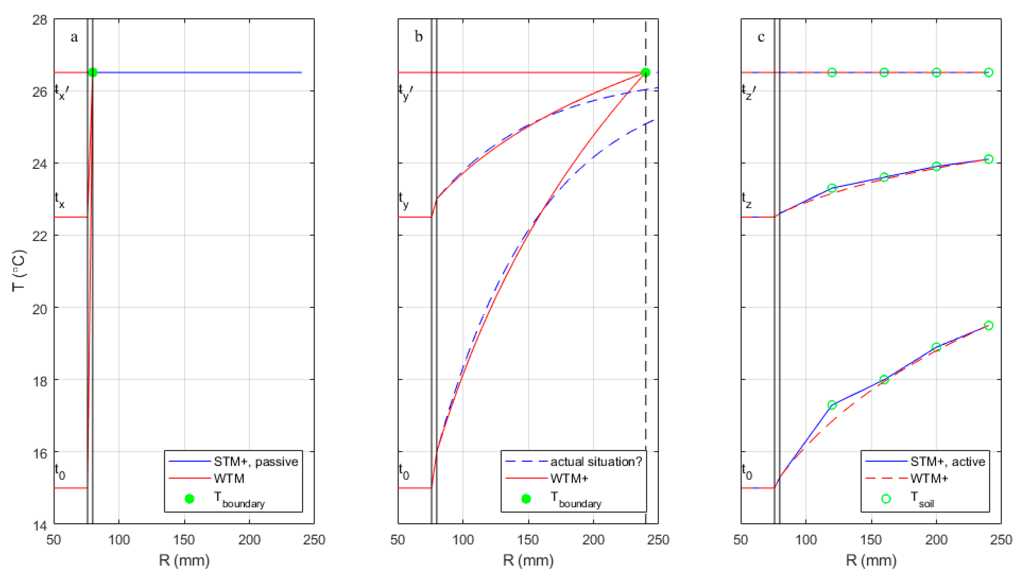
Figure 2.
ΔTN versus residence time for various diameters of PVC pipes with D3 = D2 (solid lines, TSoI = 0) and D3 = 3 × D1 (dotted lines, TSoI ≈ 1). Legend indicates nominal diameters of PVC pipes (D2). The left graph is valid for turbulent flows (Nu = 100), the right for laminar flows (Nu = 3.66).
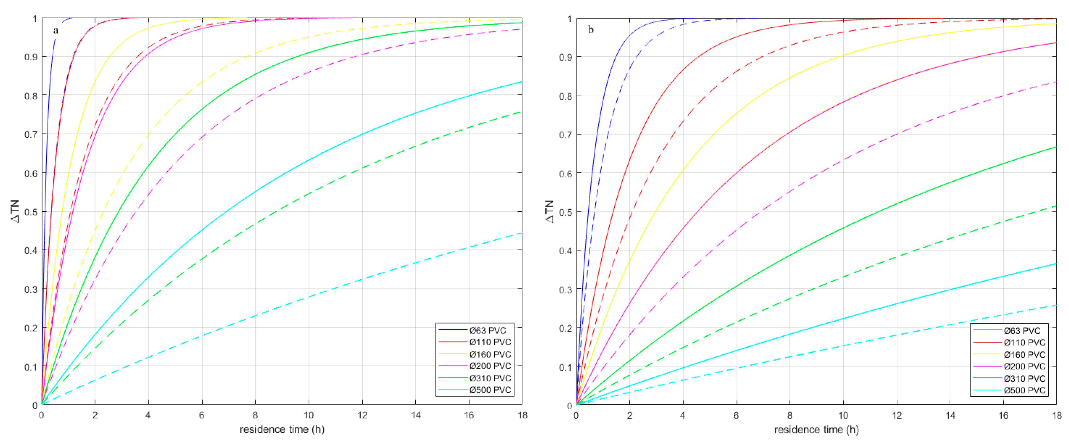
Figure 3.
Measured drinking water temperatures and modelled soil temperatures for case study 1. Indicated are the starting times of the 9 tests (see Table B1).
Figure 3.
Measured drinking water temperatures and modelled soil temperatures for case study 1. Indicated are the starting times of the 9 tests (see Table B1).
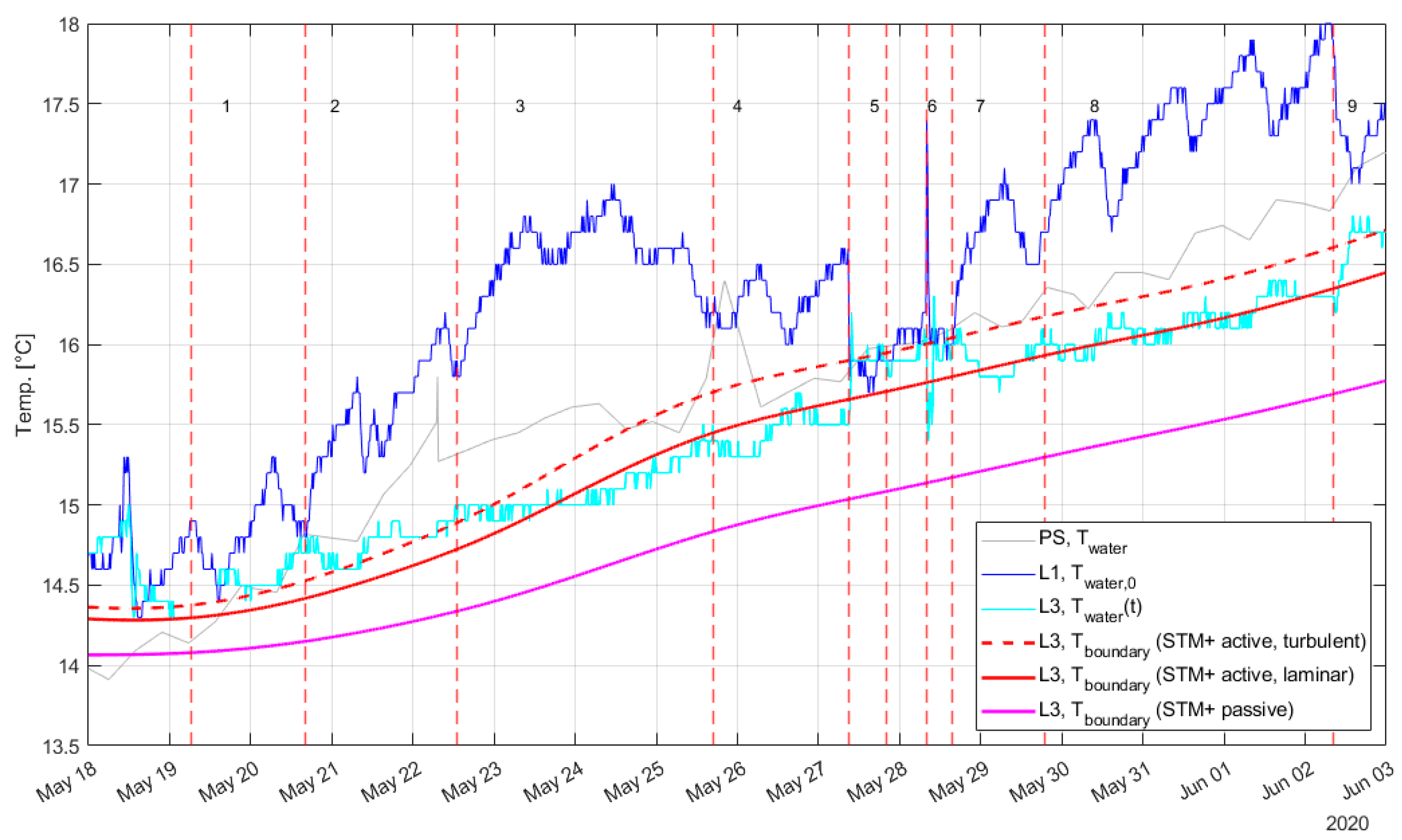
Figure 4.
ΔTN versus residence time, with Tboundary from STM+ active mode. Measured data in boxplots, where the box represents the data between the 25th and 75th percentiles, the central red lines indicate the median, and the black star indicates the average. The whiskers extend to the most extreme datapoints not considered outliers, and the outliers are plotted as red plus symbols. The curves represent Eq. (4) with different values for the TSoI. The threshold for turbulent flows is determined at Re = 5,000. Datapoints (22) with ΔTN < 0 are begin discarded. Datapoints (93) with E ≥ 0.5 are being discarded.
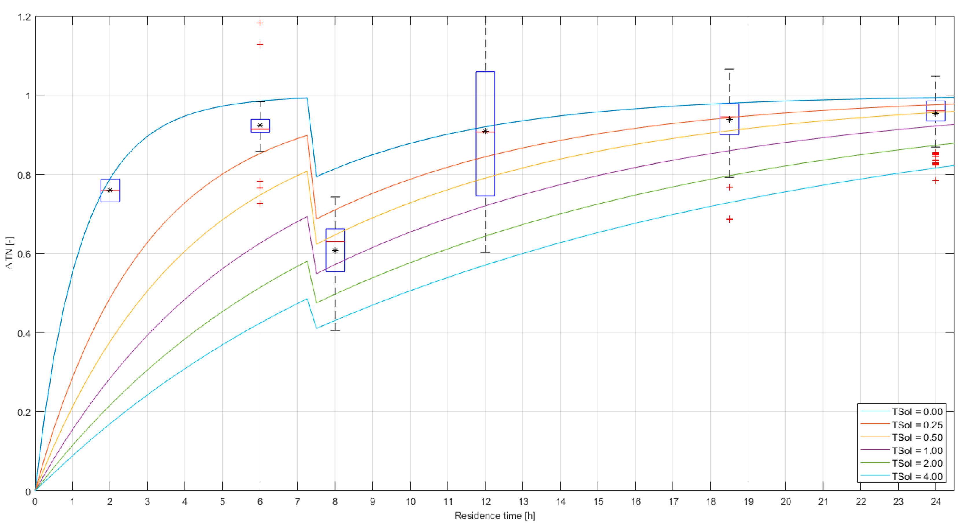
Figure 5.
Calculated TSoI for all datapoints against time (h) since start of the test. The residence time and test ID are indicated.
Figure 5.
Calculated TSoI for all datapoints against time (h) since start of the test. The residence time and test ID are indicated.
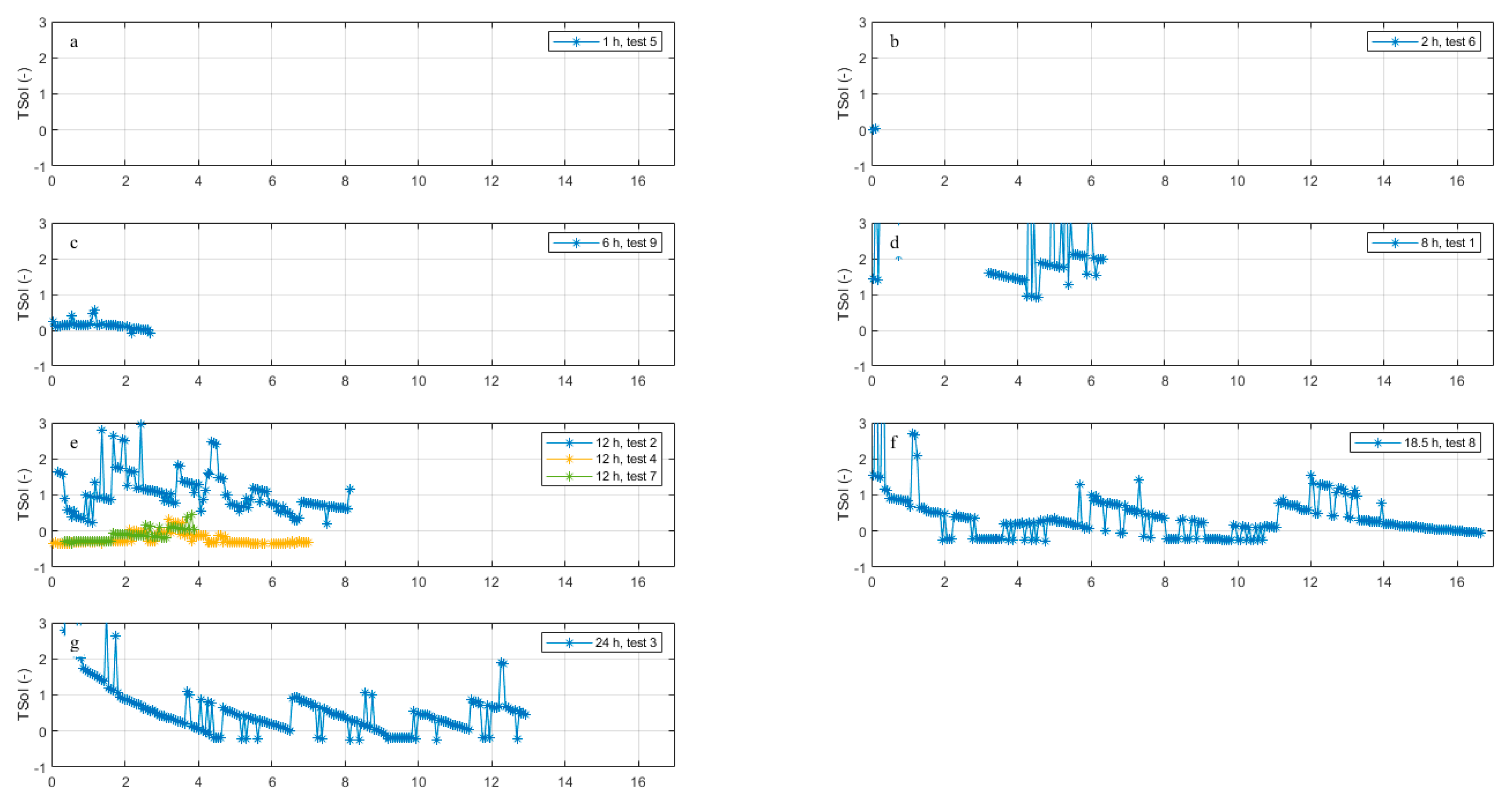
Figure 6.
Almere reservoirs (dark blue), DWDN (light blue, thin lines are distribution mains, thick lines are transport mains), DHN (red), measurement locations (white stars) and areas for analysis (green): A and B for validation and calibration, A-E for sensitivity analysis (appendix C.3).
Figure 6.
Almere reservoirs (dark blue), DWDN (light blue, thin lines are distribution mains, thick lines are transport mains), DHN (red), measurement locations (white stars) and areas for analysis (green): A and B for validation and calibration, A-E for sensitivity analysis (appendix C.3).
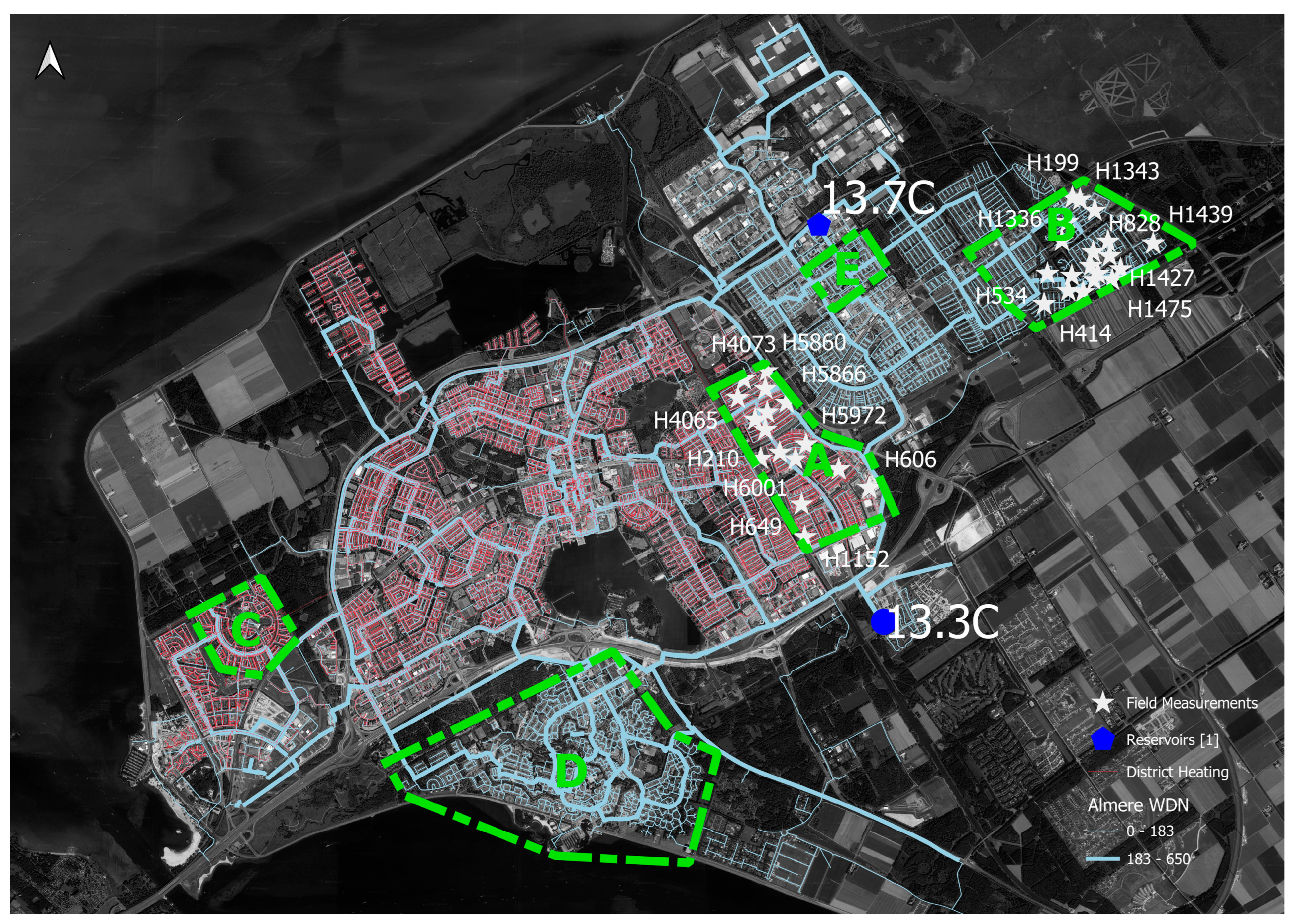
Figure 7.
Validation of WTM+, model results compared to field measurements, open circles are outliers in area A (red, below the line) and area B (blue, above the line) for (a) the base case, TSoI = 1, and (b) the optimal case with adjusted
Figure 7.
Validation of WTM+, model results compared to field measurements, open circles are outliers in area A (red, below the line) and area B (blue, above the line) for (a) the base case, TSoI = 1, and (b) the optimal case with adjusted
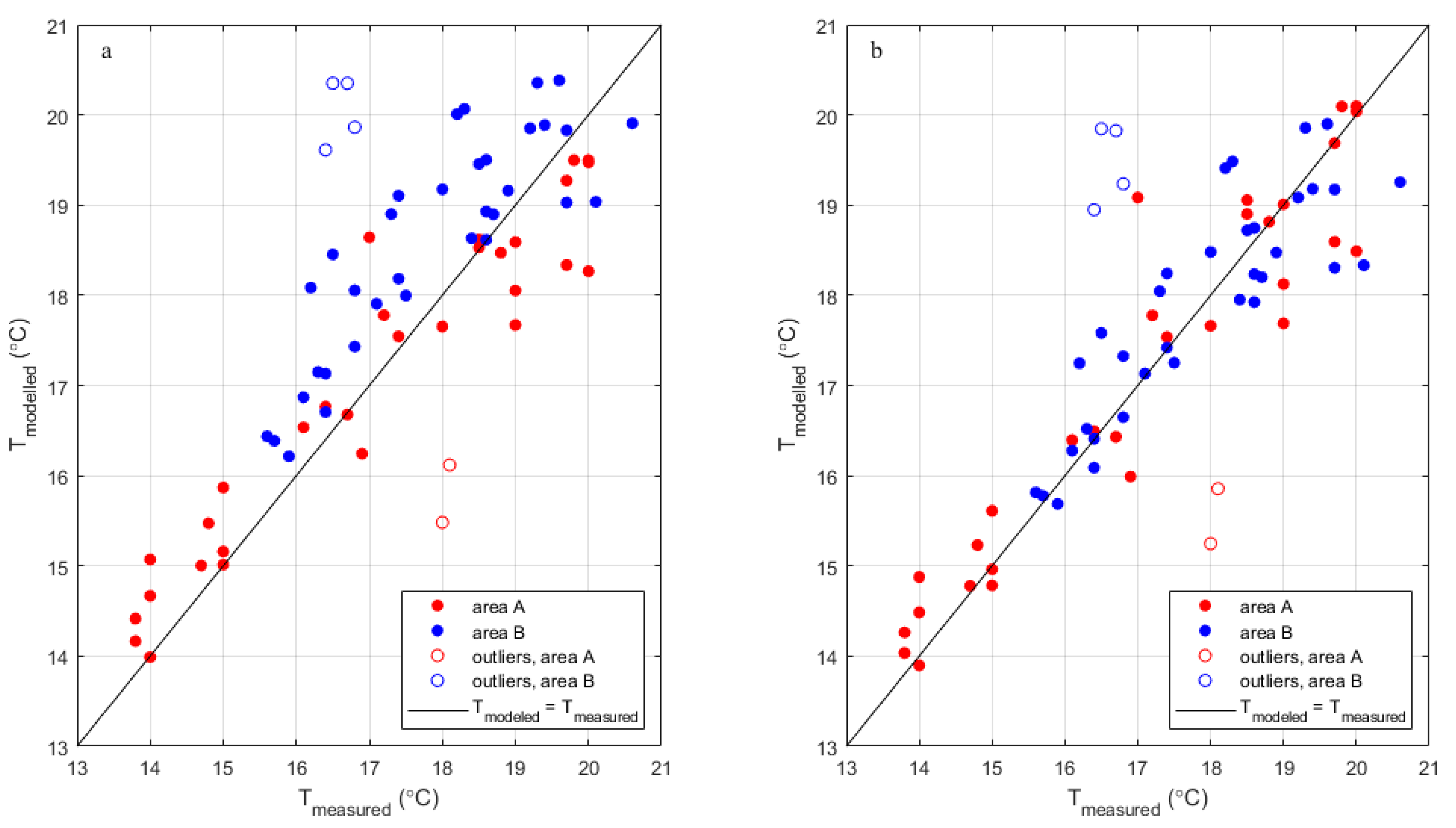
Table 1.
Settings for scenarios for the validation and calibration. Blanks are equal to the base case. Other parameter values are reported in Table C3. *The Tboundary in the optimal and extra cases are applied with Eq. (C1).
Table 1.
Settings for scenarios for the validation and calibration. Blanks are equal to the base case. Other parameter values are reported in Table C3. *The Tboundary in the optimal and extra cases are applied with Eq. (C1).
| Scenario | TSoI | TDM °C |
TDM_DHN °C |
TDM_NE °C |
TTM °C |
TTM_DHN °C |
|---|---|---|---|---|---|---|
| Base case | 1 | 18.7 | 19.5 | 20.5 | 18.0 | 20.1 |
| Optimal case | 2 | 20.1* | 20.1* | |||
| Extra cases | 0.1-10 | 18.0-21.0* | 19.0-22.0* | |||
Table 2.
Overview of case studies and recommendation for measurements.
| Case study 1 | Case study 2 | Recommendation for measurements | |
|---|---|---|---|
| Trajectory | Single pipe | DWDN | Single pipe, measure at 3 or more locations over pipe length |
| D1(mm) | 152 | 101 (51% of length) | Range of diameters |
| Length (km) | 0.9 | Ca. 700 | Result from Q and τ |
| τ(h) | 1, 2, 8, 12, 18, 24 | 5-24 | Use model to estimate the range of interest (depends on D1), measure at three or more τ, plus at very large τ. |
| Q(m3/h) | Controlled (1,4 to 0.06) | Result of demands | Use flows both in laminar and turbulent regimes |
| Duration | 2 weeks (2 h to 2 days per test) | 1 day (morning, afternoon) | 2-5 days per test |
| # datapoints | 870 (41 to 266 per test) | 72 | > 40 per test, duplicate each test |
| Water source | Surface water | Groundwater | Groundwater |
| Season | Spring | Summer | Summer, winter |
| Parameters that are known accurately | D1, D2, λsoil, λwater, λpipe, αwater, τ (Q, Re), Tboundary, Twater, Twater,0 | D1, D2, λwater, λpipe (but PVC was assumed for all pipes in the model) αwater, Twater, Twater,0 | D1, D2, λsoil, λwater, λpipe, αwater, τ, Nu, Tboundary, Twater, Twater,0 |
| Strength | Many parameters are known accurately. Parameters are constant over space. | Absolute temperature differences are significant. Parameters are constant over time. | Many parameters are known accurately. Absolute temperature differences are significant. Parameters are constant over space or time. |
| Weakness | Absolute temperature differences are small. Flow is enforced, not natural, there may not be a natural equilibrium.Nusselt not known. | Residence time and Tboundary not accurately known.Nusselt not known. |
| 1 | N.B. model results were only provided up to 3 June 2020 0:00. Therefore the last 40 datapoints of measurements were not used. |
Disclaimer/Publisher’s Note: The statements, opinions and data contained in all publications are solely those of the individual author(s) and contributor(s) and not of MDPI and/or the editor(s). MDPI and/or the editor(s) disclaim responsibility for any injury to people or property resulting from any ideas, methods, instructions or products referred to in the content. |
© 2024 by the authors. Licensee MDPI, Basel, Switzerland. This article is an open access article distributed under the terms and conditions of the Creative Commons Attribution (CC BY) license (http://creativecommons.org/licenses/by/4.0/).
Copyright: This open access article is published under a Creative Commons CC BY 4.0 license, which permit the free download, distribution, and reuse, provided that the author and preprint are cited in any reuse.


