Submitted:
15 August 2024
Posted:
16 August 2024
You are already at the latest version
Abstract
Textile heaters are made of knitted conductive yarns integrated into the fabric, making them stretchable, washable, breathable, and suitable for close-to-skin wear. The non-zero resistance in the lead wires, however, causes non-uniform power distribution, presenting a design challenge. To address this, the electrical performance of the heaters is modelled as an n-ladder resistor network. Using the finite difference method, simple, closed-form expressions are derived for networks with the power source connected to input terminals A1B1 and A1Bn, respectively. The results are exact and are used to derive approximations and design criteria. Solutions for ladder networks as presented in this paper apply to a wider class of physical problems, such as irrigation systems, transformer windings, and cooling fins.
Keywords:
heating elements
; ladder resistance network
; analytical solutions
; current distribution
1. Introduction
Heated garments have been applied to prevent hypothermia in extreme cold environments, as heat therapy for relieving joint and muscle pain, or simply as a means to increase thermal comfort. The latest advancements focus on developing all-textile heating systems that are stretchable, breathable, washable, and can be produced using existing manufacturing equipment [1,2,3]. Knitted heaters are made of lead wires composed of conductive yarns interconnected by parallel heating lines with a higher resistance. These heaters aim to provide a uniform temperature distribution, but the non-zero resistance of the lead wire sections causes more power to be dissipated near the power source connection and less further away (see Figure 1).
The decrease in heating power of a ladder-type heater system is governed by three main parameters: the resistance of the lead wire sections, the resistance of the heating lines and the number of heating lines. For the design of garments with various sizes of heaters it would be beneficial to have a simple model which interrelates those parameters.
A heating element as shown in Figure 1 can be modelled as a ladder network of series and parallel resistors, which is a well known problem in literature. In fact, ladder networks are frequently used as equivalent models for transport phenomena in systems consisting of a series of identical cells. They are thus not limited to the electrical domain but are also applicable to problems in the optical, mechanical, thermal, and chemical domains. Examples include pressure losses in irrigation systems, respiratory tissues [4], energy loss in parallel-connected streetlamps, reflectarray antennas [5], wave propagation in transmission lines [6] transformer windings [7], charge transfer in conductive polymers [8], and the heat spreading in a heat sink with cooling fins [9].
The electrical characteristics of ladder networks can be obtained by the application of Kirchoff’s laws to all elementary cells, resulting in a set of recursive relations for the node voltages, branch currents and equivalent resistance. In the past, various methods have been applied to find solutions for both finite and infinite ladder networks, including the use of Fibonacci sequences [10], Z-transforms [11], Green’s functions [12], and the recursion-transform method [13,14]. As the number of cells in the ladder network increases, the number of equations also increases and either rigorous recursive circuit equations have to be solved or complex state-space matrices need to be handled resulting in rapidly increasing computational costs [7]. It would therefore be useful to be able to express the results in simple-to-use analytical expressions. Solving the difference equation for the unit cell, Mondal [7] derived generalized analytical expressions for the electrical characteristics of finite homogeneous ladder networks. Generalized analytical expressions for the electrical characteristics of finite homogeneous ladder networks are available, but they are often lengthy despite being in closed form. In this paper, we will derive more compact and user-friendly solutions, and apply these to obtain asymptotic expressions and design criteria. While this work focuses on purely resistive networks, the solutions can be easily extended to resistor-inductor-capacitor networks by substituting the resistances with the corresponding complex impedances. [6,7].
2. Theory
2.1. Layout and Definitions for Ladder Configuration
We consider a sequence of n heaters with resistance Rh which are connected by two lead wire lines, A and B, resulting in n-1 lead wire parts with resistance RA, and RB, respectively (see Figure 2). A potential V0 is applied over nodes A1 and B1 The currents in the lead wires and heater resistances are indicated with iA,k , iB,k and ih,k respectively.
Applying Kirchov’s Voltage Law (KVL) to segment k, we obtain
| Eq.1 |
Then, using
| Eq.2 |
and introducing the lead wire resistance ratio as ε = (RA+ RB)/Rh we can rewrite Eq.1 as
| Eq.3 |
This is a second order finite difference equation for which , or combinations thereof are known solutions. Here we use as a trial function
| Eq.4 |
Inserting this in Equation (3) then results in and C = 0. The coefficients A and B then follow from applying the KVL to the first and the last mesh:
which can be rewritten as
| Eq.5 |
The solution for A and B then follows by substituting the trial solution in Equation (5). These solutions can be simplified by using the addition formulas for hyperbolic functions. Solving for A and B then gives
from which we obtain
| Eq.6 | |
| Eq.7 |
Here denotes the equivalent resistance of the ladder heater configuration and I0 the total current through the heater. The lead wire and heater currents in Equation (7) result in compact closed-form equations with the node number, k, and the total number of heater wires, n, as the main parameters. With this formulation it can immediately be seen that the lead wire current decreases from I0 at k=0 (near the source) to 0 at the end (k=n). The heater current starts at V0/Rh at k=1, as expected.
2.2. Solution for Diagonal Configuration
In what we call the diagonal configuration we connect the power source to nodes A1 and Bn, respectively (see Figure 3). The solution procedure is similar to that for the ladder configuration, except that we now have
| Eq.8 |
From symmetry considerations we can see that i,A,1 = iB,n-1 and similarly for the other node numbers. In addition, for the heater currents, we have ih,k = ik,n-k+1.
Applying Equation (8) in the governing KVL equation for the kth mesh (Equation (3)) we get
| Eq.9 |
The boundary condition is obtained by applying the KVL over the power source connections:
| Eq.10 |
Because of the symmetry we now propose as trial function
| Eq.11 |
Applying this to Equation (11) then gives and . By combining Equation (8) and Equation (11) we get
and hence we find A=0. From we find . From Equation (10) and Equations A2 and A3 we get and, finally
| Eq.13 | ||
| Eq.14 | ||
The expressions in Equations (13) and (14) are simpler and more condensed than those reported by Mondal [7]. Direct inspection shows that decreases to 0 at the last branch, k = n, and that the heater currents are symmetric around (n+1)/2.
2.3. Simplified Solutions
The above expressions are exact and can be simplified by assuming that . In that case we obtain for the parameter δ:
| Eq.15 |
For ε < 0.4 the error by neglecting the second an subsequent terms is less than 0.01. Further simplification by Taylor series development, however, do not result in practical results since the arguments of the sinh functions scale as nδ which in this case is of order unity or larger.
The equivalent resistances are important parameters for calculating the overall current and power dissipated by the network. For small ε the equivalent resistances should converge to the solution of a parallel resistor network Rh/n. In addition for we obtain for the equivalent ladder and diagonal resistances:
| Eq.16 |
For the diagonal configuration we may approximate the solutions for the lead wire and heater currents as
| Eq.17 |
2.4. Design Criteria
In this paper we aim to minimize the difference between dissipated heat in the different heating wires. That means that we have to consider the individual heating powers: . For the ladder configuration this means that the ratio between minimum and maximum current must be larger than a certain value f. As a measure of the uniformity we define the heater current decay criterion rhc as:
| Eq.18 |
For the ladder and diagonal configuration these ratios amount to respectively
| Eq.19 |
in which we introduced the approximation Equation (15) for convenience. For the second criterion, we consider the heat generated by the different sections of the lead wires. Figure 6 and Figure 8 show that the generated heat is largest close to the power connections and decreases further downstream. For our application, a knitted heater structure, it is no problem that the lead wires also contribute to the heating but we should ensure that the power of the lead wires does not exceed that of the heater wires. Therefore, we require that the maximum lead wire power is always equal or smaller than that of the heater wires
| Eq.20 |
Again using Equation (7) and 14, we obtain with some rewriting
| Eq.21 |
Note that from the latter equation, it can be deduced that the criterion is met if
| Eq.22 |
3. Example Cases
In order to validate our closed form expressions we will compare it with numerical simulations (using MatLab Simulink). In addition we will show how the approximations discussed in section 2.3 relate to these exact solutions. For this we will consider a typical case for a knitted heater strip and assume V0 = 10 V, Rh = 100 Ω and RA = RB = 1, 5 or 10 Ω, resulting in ε values of 0.02, 0.10 and 0.20, respectively.
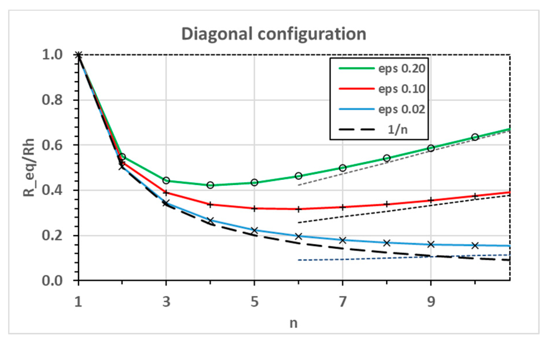
First we consider the equivalent resistances as given by Equation (6) and 13 and their approximations, Equation (16). As shown in Figure 4 for the ladder configuration the equivalent resistances decrease monotonically with increasing n until they reach their asymptotic value given by the first of Equation (16). For small ε the curves approximate the 1/n limit of the parallel resistor configuration. The closed form solutions (full lines) and simulation results agree exactly. The approximations obtained by substituting δ = √ε (Equation (15)) almost coincide with the full solution (maximum deviation 0.65%) and can thus be considered as an accurate and practical simplification. The equivalent resistance of the diagonal configuration on the other hand, first follows an 1/n decay which is later taken over by the asymptotic increase (2nd of Equation (16)). The asymptotes (shown as the intermittent lines in Figure 5) are shown to converge well with the closed form solutions (full lines) and the simulations (symbols).
The currents in the lead wires and heaters (Equation (7)) are depicted in Figure 6 and 7 for 5, 10 and 15 heater wires with an ε value of 0.02 (colored full lines), and for ε values of 0.10 and 0.20 (dashed lines). The simulated values (symbols) agree exactly with the closed form expressions in all considered cases. The lead wire currents are maximum near the power source and vanish at k = n. The heater currents (Figure 7) always start at a value of V0/Rh at k=1. The curves have a parabolic shape and a minimum at k = n.
Figure 6.
Lead wire currents for ladder configuration. Lines are exact solutions, symbols are Simulink data.
Figure 6.
Lead wire currents for ladder configuration. Lines are exact solutions, symbols are Simulink data.
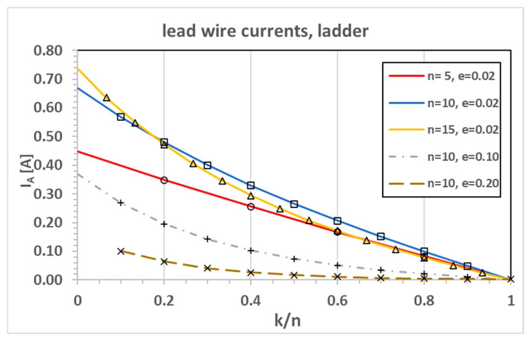
Figure 7.
Heater currents for ladder configuration. Lines are exact solutions, symbols are Simulink data.
Figure 7.
Heater currents for ladder configuration. Lines are exact solutions, symbols are Simulink data.
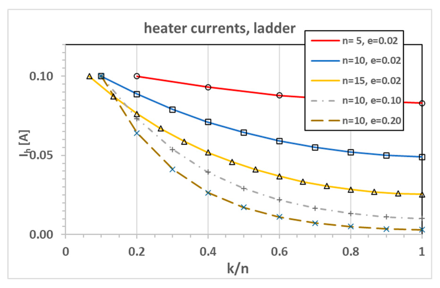
Figure 8.
Lead wire currents for diagonal configuration. Lines are exact solutions, symbols are Simulink data and dashed lines are approximations.
Figure 8.
Lead wire currents for diagonal configuration. Lines are exact solutions, symbols are Simulink data and dashed lines are approximations.
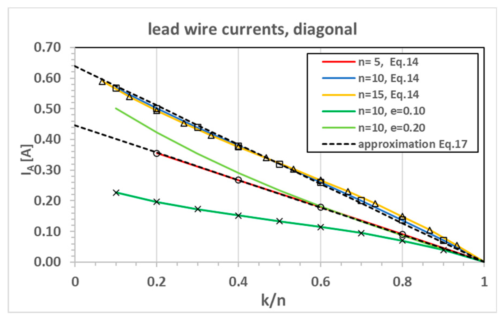
Figure 9.
Heater currents for diagonal configuration. Lines are exact solutions, symbols are Simulink data. Dashed lines are the approximation according to Equation (17).
Figure 9.
Heater currents for diagonal configuration. Lines are exact solutions, symbols are Simulink data. Dashed lines are the approximation according to Equation (17).
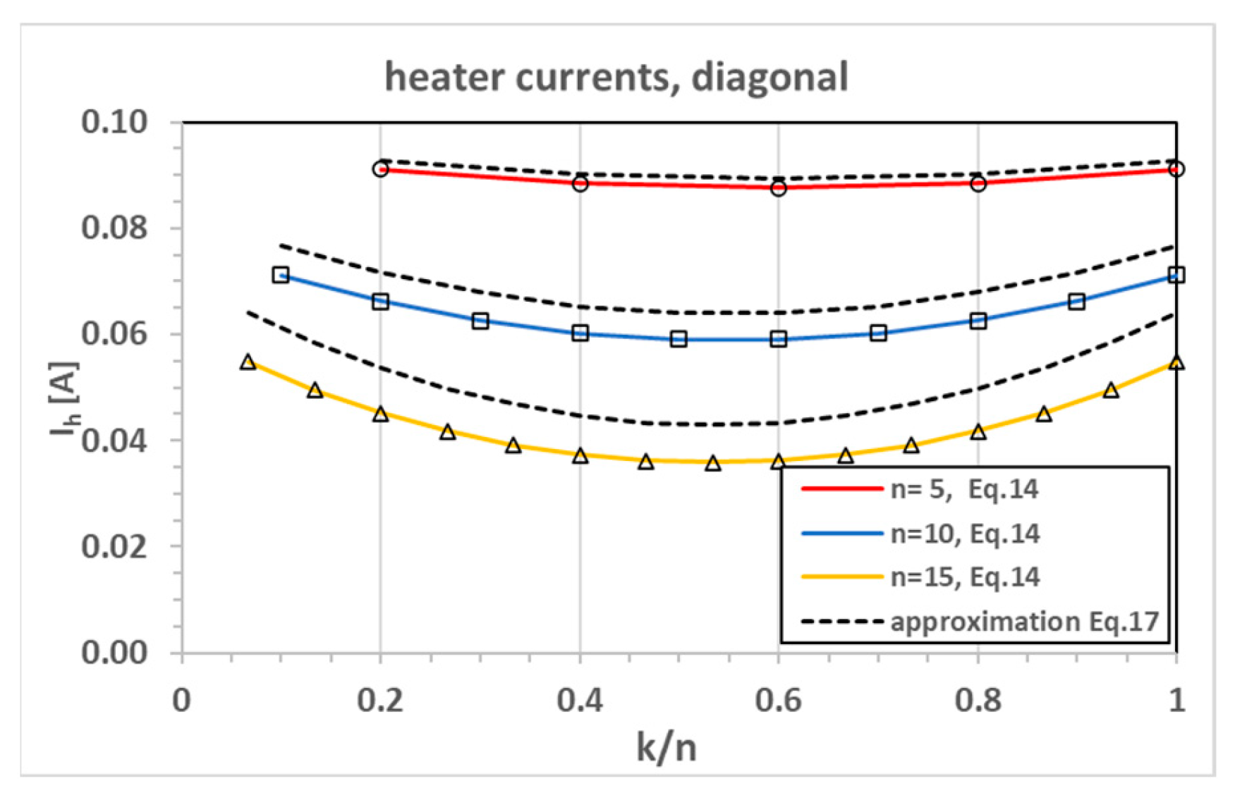
Figure 8 and Figure 9 show similar plots for the diagonal configuration. In that case, the lead wire currents (Figure 8) show a more linear behavior and Equation (17) (dashed lines) turn out to give good approximations. The heater currents have a minimum at and show much more uniformity over the different heater nodes as compared to the ladder currents. The approximations now deviate more from the exact solutions.
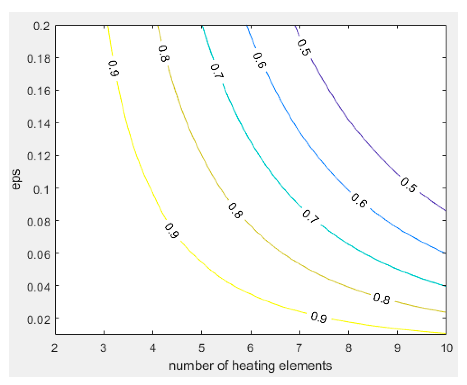
In Figure 10 and 11 we present the uniformity criterion for the ladder and diagonal cases. A uniformity of unity signifies that all heating wires have equal temperatures, which is only achievable in the ideal cases of ε=0 or n=1. For a configuration with 10 heaters, a uniformity value of 0.5 would require an ε value of 0.09 for the diagonal case and a value of 0.02 for the ladder case, indicating that in the latter case a 4.5 times lower lead wire resistance would be needed.
Figure 10.
Contour plot for criterion Equation (18), Ladder configuration.
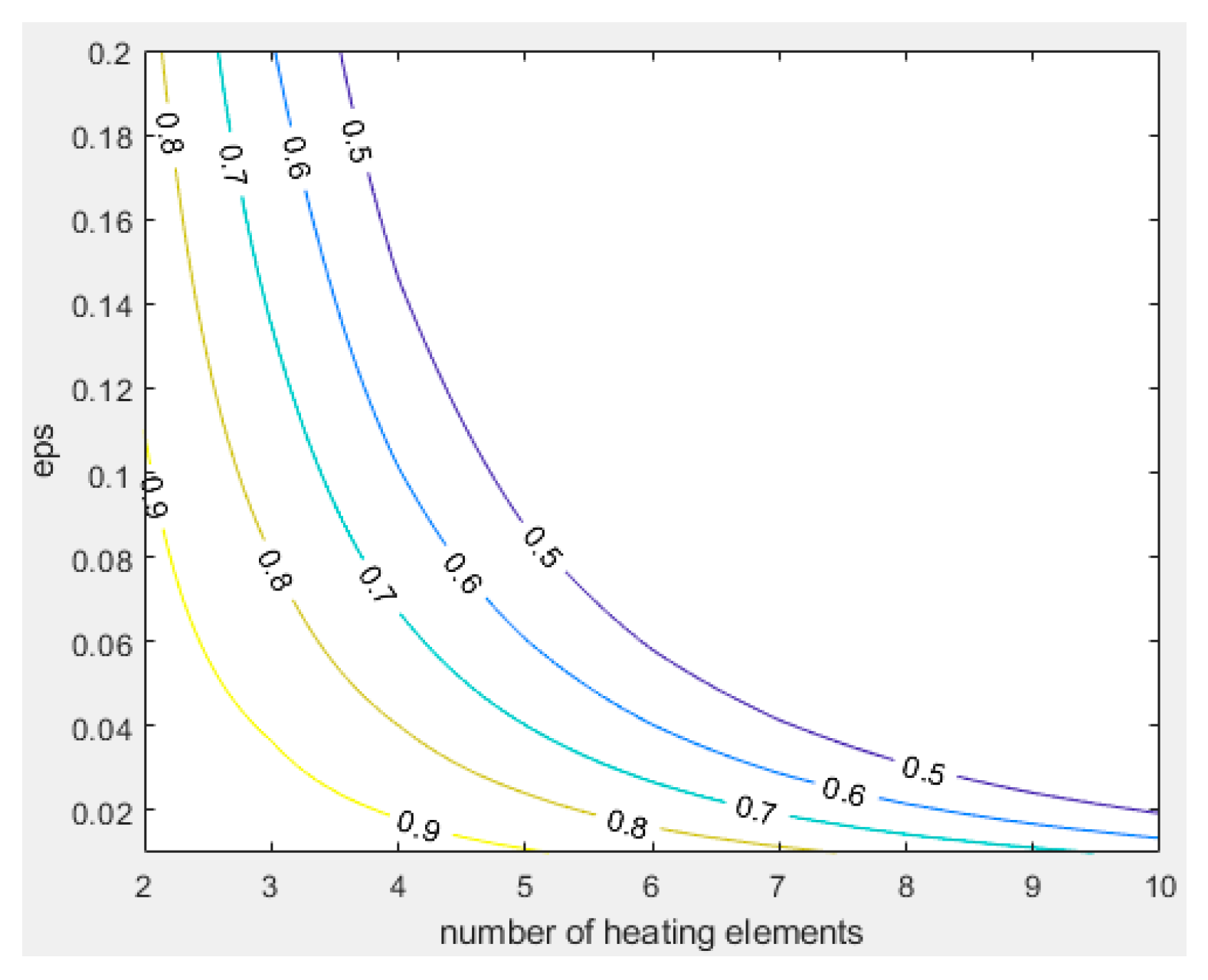
Figure 11.
as Figure 10, Diagonal configuration.
Figure 11.
as Figure 10, Diagonal configuration.
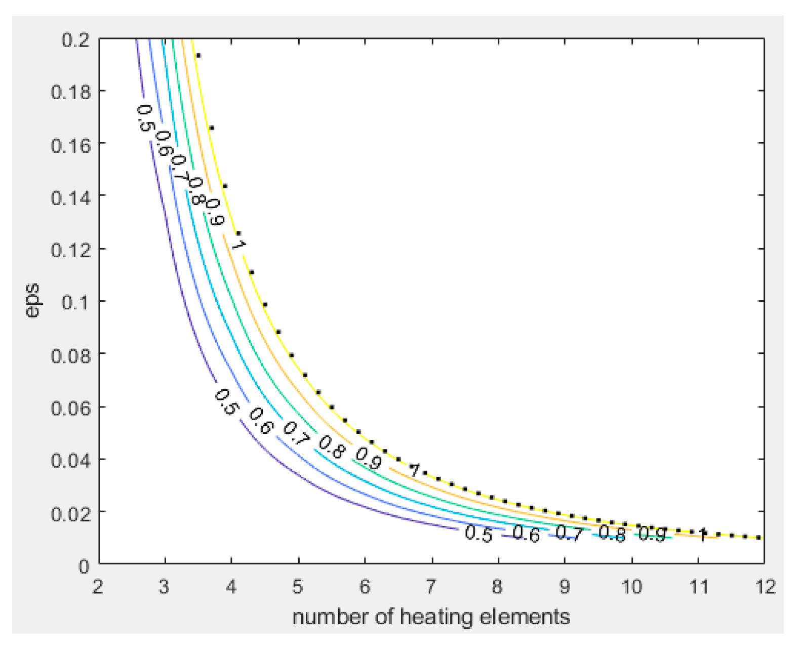
The plots for the 2nd criterion are depicted in figures 11 and 12. Of practical importance is the case where the maximum heat generated by the lead wires matches that of the heaters maximum, i.e., . Assuming that we have a lead wire resistance of a fixed minimum value, we can use this criterium to calculate the maximum number of heaters in relation to a chosen heater resistance. With lead wire resistances of 1 Ω and a heater resistance of 100 Ω we obtain an ε of 0.02 and thus can have no more than 12, respectively 9 heaters for the ladder and diagonal configurations.
Figure 11.
Contour plot for criterion Equation (20), Ladder configuration.
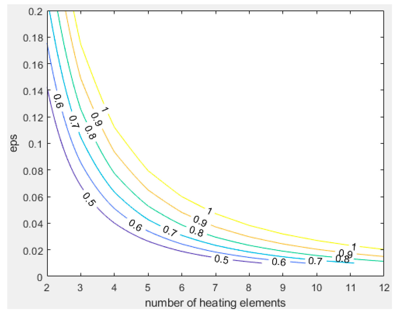
Figure 12.
as Figure 11, Diagonal configuration. The dots are according to Equation (22).
Figure 12.
as Figure 11, Diagonal configuration. The dots are according to Equation (22).
4. Discussion and Conclusions
This paper presents simple closed-form solutions for the electrical characteristics of finite homogeneous ladder networks with the power source connected to input terminals A1B1 and A1Bn, respectively. Explicit expressions are derived for the equivalent resistances and mesh currents and based on those, approximations and asymptotic solutions are presented. In addition, we formulated two criteria: one for the uniformity of the current distribution over the heating wires, and one to ensure that the power dissipated in the lead wires does not exceed that of the heater wires. The solutions are derived for purely resistive networks but can be generalized to ladder networks consisting of combinations of resistances, inductances and capacitances if the lead wire and heater resistances are replaced with equivalent impedances.
Appendix A
For the evaluation of Equation (10) we use the sum of power identities
| Eq.A1 |
Applying this to the hyperbolic functions eventually leads to
| Eq.A2 | |
| Eq.A3 |
Note that for m=n-1 the sinh term in Equation A2 vanishes and the corresponding cosh term in Eq.A3 reduces to unity.
References
- Saidi, A.; Gauvin, C.; Ladhari, S.; Nguyen-Tri, P. Advanced Functional Materials for Intelligent Thermoregulation in Personal Protective Equipment. Polymers 2021, 13, 3711. [Google Scholar] [CrossRef] [PubMed]
- Tabor, J.; Chatterjee, K.; Ghosh, T.K. Smart Textile-Based Personal Thermal Comfort Systems: Current Status and Potential Solutions. Adv. Mater. Technol. 2020, 5, 1901155. [Google Scholar] [CrossRef]
- Roh, J.-S.; Kim, S. All-fabric intelligent temperature regulation system for smart clothing applications. J. Intell. Mater. Syst. Struct. 2015, 27, 1165–1175. [Google Scholar] [CrossRef]
- Ionescu, C.M.; Machado, J.A.T.; De Keyser, R. Modeling of the Lung Impedance Using a Fractional-Order Ladder Network With Constant Phase Elements. IEEE Trans. Biomed. Circuits Syst. 2010, 5, 83–89. [Google Scholar] [CrossRef] [PubMed]
- Hum, S.V.; Du, B. Equivalent Circuit Modeling for Reflectarrays Using Floquet Modal Expansion. IEEE Trans. Antennas Propag. 2017, 65, 1131–1140. [Google Scholar] [CrossRef]
- Smith, P.W. , Transient electronics : pulsed circuit technology. 2002, J. Wiley: Chichester ;
- Mondal, M.; Kumbhar, G.B. Generalized analytical formulae to compute electrical characteristics of a homogenous ladder network of the transformer winding. Int. J. Circuit Theory Appl. 2018, 46, 911–925. [Google Scholar] [CrossRef]
- Nagashima, H.N.; Onody, R.N.; Faria, R.M. ac transport studies in polymers by resistor-network and transfer-matrix approaches: Application to polyaniline. Phys. Rev. B 1999, 59, 905–909. [Google Scholar] [CrossRef]
- Farkas, G. , Fundamentals of Thermal Transient Measurements, in Theory and Practice of Thermal Transient Testing of Electronic Components, M. Rencz, G. Farkas, and A. Poppe, Editors. 2022, Springer International Publishing: Cham. p. 171-208.
- Faccio, M.; Ferri, G.; D'Amico, A. A new fast method for ladder networks characterization. IEEE Trans. Circuits Syst. 1991, 38, 1377–1382. [Google Scholar] [CrossRef]
- Dutta Roy, S.C. , Difference Equations, Z-Transforms and Resistive Ladders, in Circuits, Systems and Signal Processing: A Tutorials Approach. 2018, Springer Singapore: Singapore. p. 135-140.
- Cserti, J. Application of the lattice Green’s function for calculating the resistance of an infinite network of resistors. Am. J. Phys. 2000, 68, 896–906. [Google Scholar] [CrossRef]
- Tan, Z.-Z., J. H. Asad, and M.Q. Owaidat, Resistance formulae of a multipurpose n-step network and its application in LC network. International Journal of Circuit Theory and Applications, 2017. 45(12): p. 1942-1957.
- Zhou, S.; Wang, Z.-X.; Zhao, Y.-Q.; Tan, Z.-Z. Electrical properties of a generalized 2 × n resistor network. Commun. Theor. Phys. 2023, 75, 075701. [Google Scholar] [CrossRef]
Figure 1.
Thermal image of a knitted textile heater.
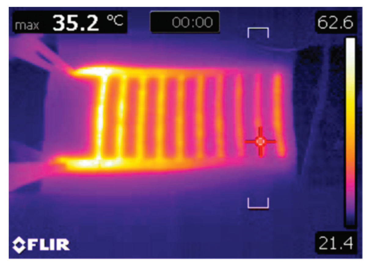
Figure 2.
Resistances for the ladder configuration with input terminals connected to A1B1.
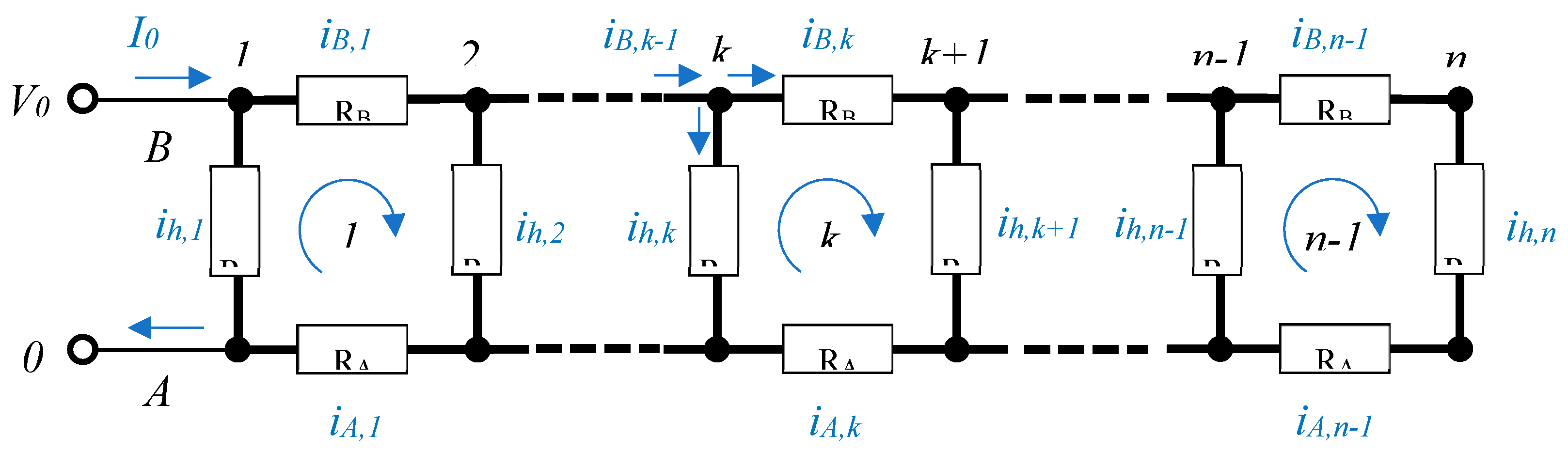
Figure 3.
Resistances for the diagonal configuration with input terminals connected to A1Bn.
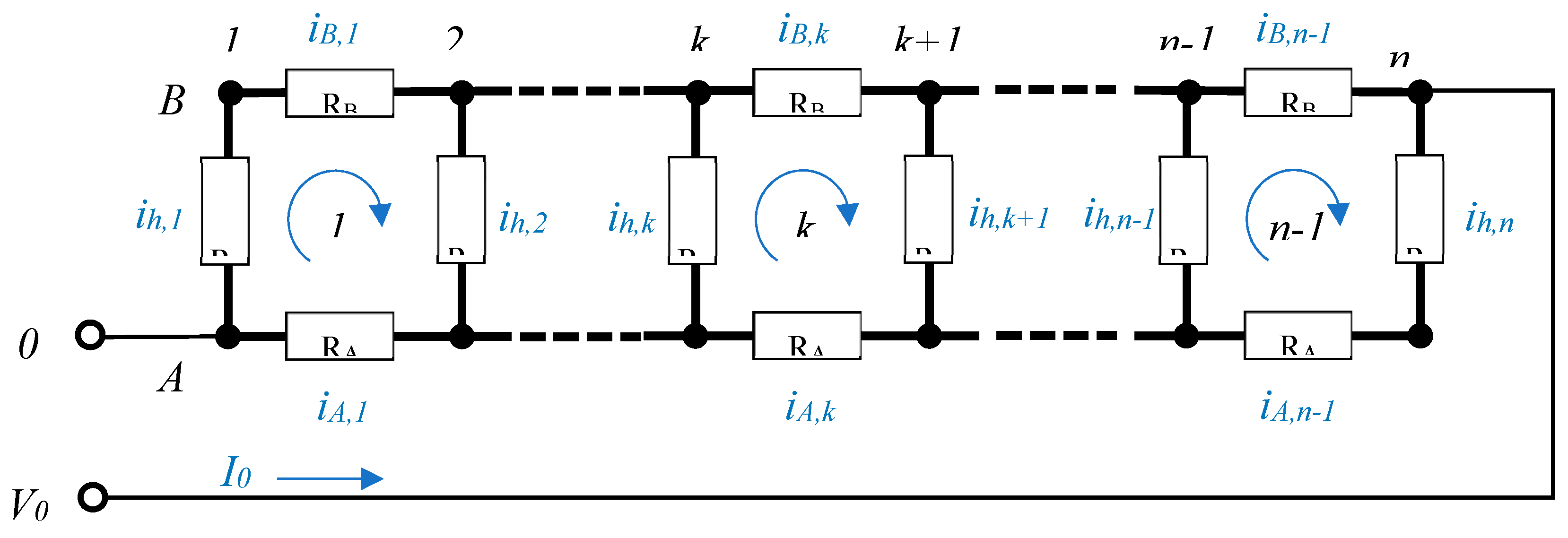
Figure 4.
Equivalent resistances for ladder configuration. Full lines are exact solutions, symbols are Simulink data, dashed lines are limiting solutions.
Figure 4.
Equivalent resistances for ladder configuration. Full lines are exact solutions, symbols are Simulink data, dashed lines are limiting solutions.
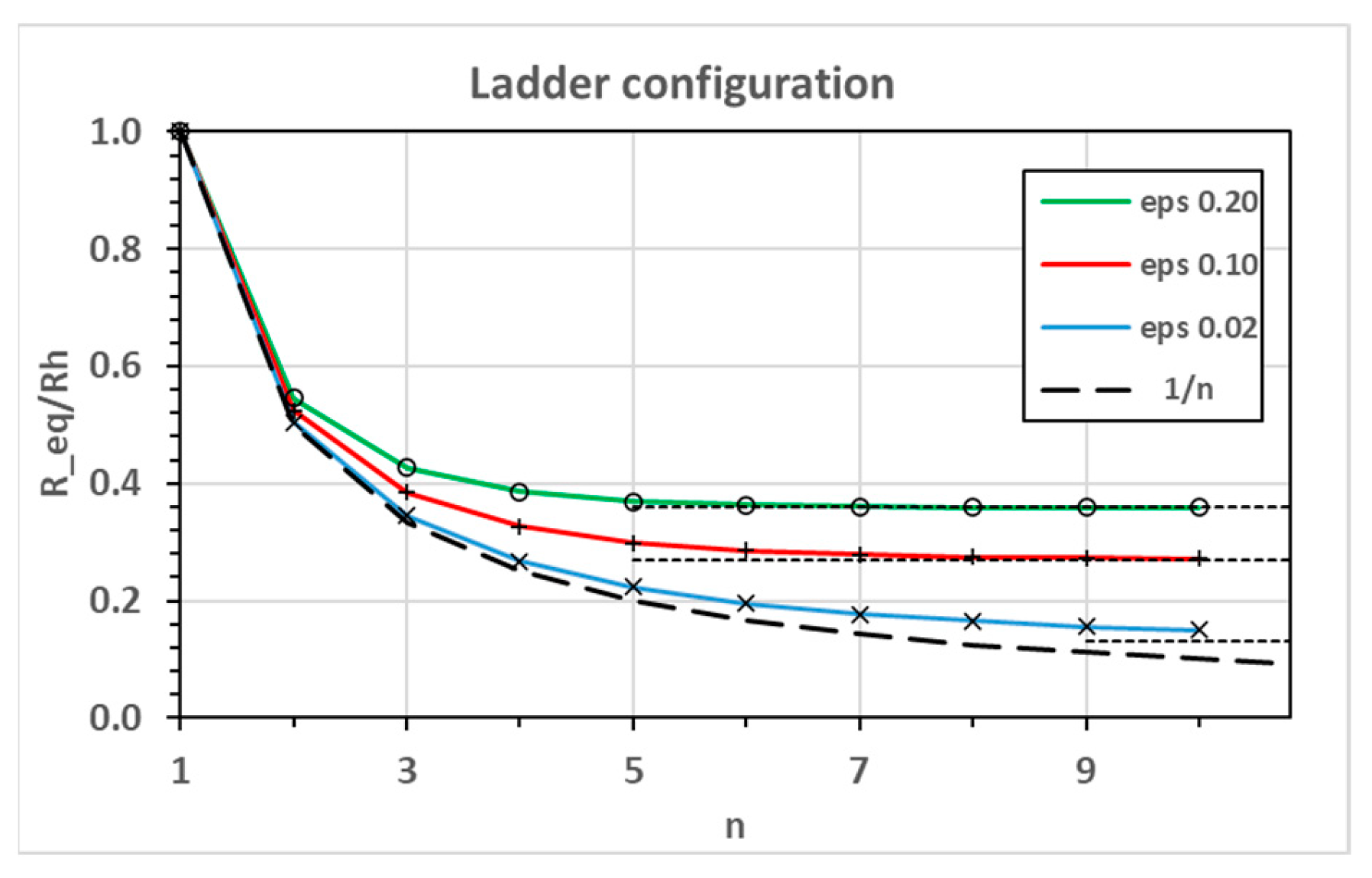
Figure 5.
Equivalent resistances for diagonal configuration. Full lines are exact solutions, symbols are Simulink data, dashed lines are limiting solutions.
Figure 5.
Equivalent resistances for diagonal configuration. Full lines are exact solutions, symbols are Simulink data, dashed lines are limiting solutions.
Disclaimer/Publisher’s Note: The statements, opinions and data contained in all publications are solely those of the individual author(s) and contributor(s) and not of MDPI and/or the editor(s). MDPI and/or the editor(s) disclaim responsibility for any injury to people or property resulting from any ideas, methods, instructions or products referred to in the content. |
© 2024 by the author. Licensee MDPI, Basel, Switzerland. This article is an open access article distributed under the terms and conditions of the Creative Commons Attribution (CC BY) license (https://creativecommons.org/licenses/by/4.0/).
Copyright: This open access article is published under a Creative Commons CC BY 4.0 license, which permit the free download, distribution, and reuse, provided that the author and preprint are cited in any reuse.


