
Submitted:
13 August 2024
Posted:
14 August 2024
You are already at the latest version
Abstract
In the modern days the data is coming from various devices like mobiles, tabs, laptops, computers, IOT devices e.tc and is stored in the electronics form in the systems using the concept of files or data bases. Clustering Technique is used to extract data from these sources. Improving the accuracy of the model is improved using the feature selection or feature engineering or both. The feature engineering is used to add a new feature based on the global mean. Along with that new feature in addition to the feature selection increase the overall accuracy of the model.
Keywords:
Clustering
; Clustering Algorithms
; Distance metrics
; classification
; Feature selection
; Feature Engineering
; Accuracy
; Confusion matrix
I. Introduction
Clustering and classification
Unsupervised machine learning techniques such as clustering are used to classify similar data points into groups or clusters according to their shared attributes. Ensuring that data points inside a cluster are more comparable to one another than to those in other clusters is the aim. Numerous disciplines, including data mining, pattern recognition, image analysis, and bioinformatics, make extensive use of this technique. Based on how they handle data grouping, clustering techniques can be divided into different categories. The following are a few of the most popular kinds of clustering methods:
1. Partitioning Clustering:
a. K-Means: By reducing the variation within each cluster, the Kmeans algorithm divides the data into k clusters. Iteratively matching each data point to the closest centroid, it begins with k initial centroids and updates the centroids according to the average of the points in each cluster[2].
b. K-Medoids (PAM): It is a K-Means version in which the cluster centers are the actual data points (medoids) rather than the mean of the points. In contrast to K-Means, it is less susceptible to outliers [3].
2. Hierarchical Clustering [4]:
a. Agglomerative Clustering: Beginning with each data point as its own cluster, this bottom-up method repeatedly combines the closest pairings of clusters until either a single cluster forms or a halting condition is satisfied.
b. Divisive Clustering: Each data point in this bottom-up method begins as its own cluster, and repeatedly merges the closest pairings of clusters until either a single cluster forms or a halting requirement is satisfied.
3. Density-Based Clustering:
a. Density-Based Spatial Clustering of Applications with Noise(DBSCAN): It classifies points in low-density regions as outliers and groups points that are densely packed together, or in high-density regions. It is especially helpful for data that have asymmetrical shapes [5].
b. OPTICS (Ordering Points To Identify the Clustering Structure): By generating a reachability plot, it extends DBSCAN by offering a more adaptable method of locating clusters and outliers [6].
4. Model-Based Clustering:
a. Gaussian Mixture Models (GMM): It is assumed that a combination of multiple Gaussian distributions is used to generate the data points. It clusters data points according to probability and estimates the parameters of these distributions using the Expectation-Maximization (EM) algorithm [7].
b. Latent Dirichlet Allocation (LDA): LDA is frequently used in topic modeling, where it is assumed that subjects are mixtures of words and that documents are mixtures of topics. Documents can be grouped according to their underlying topics[8].
5. Grid-Based Clustering:
a. Statistical Information Grid (STING): It creates a grid out of the data space and clusters the data according to statistical data in each grid cell. It is efficient for large datasets and allows for multi-resolution clustering [9].
b. CLIQUE (CLustering In QUEst): Combines grid-based and density-based approaches by identifying dense regions in a grid-based representation and clustering them[10].
6. Fuzzy Clustering:
a. Fuzzy C-Means: Fuzzy clustering permits each data point to belong to numerous groups with different degrees of membership, in contrast to hard clustering techniques like K-Means. The overall weighted distance between the data points and the cluster centers is what the algorithm seeks to minimize [11].
7. Spectral Clustering:
It reduces dimensionality by using similarity matrix eigenvalues before using clustering algorithms like K-Means. It can effectively capture complicated structures in the data and is useful for clustering non-convex shapes. Every clustering technique has advantages and disadvantages of its own, and the best technique will rely on the particulars of the data as well as the analysis's objectives [12].
Clustering Advantages & Disadvantages [13]
Clustering Advantages
a. Unsupervised Learning: Since labelled data is not necessary for clustering, it can be used for exploratory data analysis in situations when labels are not available.
b. Identifying Patterns: It assists in locating hidden structures and patterns in the data, which might produce insightful discoveries.
c. Data Reduction: By putting related things together, clustering can simplify analysis and lessen the complexity of the data.
c. Versatility: Applications for clustering can be found in many fields, including image processing, social network analysis, and market segmentation.
d. Anomaly Detection: It can be applied to network security and fraud detection to find anomalies or outliers in the data.
e. Data Summarization: By depicting data as a small number of clusters rather than a large number of individual points, clustering aids with data summarization.
Clustering Disadvantages
a. Determining the Number of Clusters: Numerous clustering algorithms, such as K-means, necessitate knowing the number of clusters ahead of time, which is frequently unknown.
b. Scalability: When dealing with huge datasets, several clustering techniques struggle to scale and end up consuming a lot of computer power.
c. Sensitivity to Initialization: Different results can be obtained using methods such as K-means because of their sensitivity to the initial placement of centroids. Handling diverse Shapes and Sizes: Some algorithms, like K-means, may not work well with clusters of diverse shapes and sizes since they presume that the clusters are spherical.
d. High Dimensionality: The curse of dimensionality, when distance measures lose significance, makes clustering in high-dimensional spaces difficult.
e. Interpretability: In complex or high-dimensional datasets, the outcomes of clustering might occasionally be difficult to understand.
f. Noise and Outliers: The quality of the clusters produced by clustering algorithms can be impacted by noise and outliers.
Examples of Specific Advantages and Disadvantages for Common Clustering Algorithms
K-means:
Advantages: It is easy to use, effective with big datasets, and performs best with spherically shaped, similarly sized clusters.
Disadvantages: expects spherical clusters and calls for the specification of the number of clusters. It is also sensitive to initialization and outliers.
Hierarchical Clustering:
Advantages: Does not require the number of clusters to be specified, produces a dendrogram that is easy to interpret, and can find arbitrarily shaped clusters.
Disadvantages: Computationally expensive, especially for large datasets, and sensitive to noise and outliers.
DBSCAN:
Advantages: It finds clusters of any shape, doesn't need the amount of clusters to be provided, and performs well with noise.
Disadvantages: It struggles with high-dimensional data and clusters of different densities; parameter selection (epsilon and minPts) determines how well it performs.
Gaussian Mixture Models (GMM):
Advantages: It can be more adaptable than K-means and model clusters of various sizes and forms. It also offers probabilistic cluster assignments.
Disadvantages: It is sensitive to initialization, computationally demanding, and requires the number of clusters to be supplied.
Classification[14]
Classification is a supervised machine learning method that uses a training dataset of observations with known class labels to predict the category or class label of fresh observations. Developing a model that correctly assigns class labels to novel, unseen examples is the main goal of categorization. This is extensively utilized in a number of industries, including marketing, healthcare, and finance.
Classification Key Characteristics
Supervised Learning: Labeled data is necessary for classification, meaning that every example in the training set has a known class label attached to it.
Discrete Output: A discrete label, such as spam or not, or a multi-class label like several flower species, is the result of a classification model.
Training and Testing: To gauge the model's performance, it is trained on a training dataset and tested on a testing dataset.
Common Classification Algorithms
1. Linear Models
a. Logistic Regression: Estimates probabilities using a logistic function and classifies observations based on a threshold [15].
b. Linear Discriminant Analysis (LDA): Finding a linear combination of features that distinguishes between classes is based on the assumption of normally distributed data and equal covariance matrices [16].
2. Tree-Based Models
a. Decision Trees: Based on feature values, it divides the data into subsets and creates a tree with a class label for each leaf [17].
b. Random Forests: a group of decision trees that, by reducing overfitting and averaging predictions, increase classification accuracy [18].
c. Gradient Boosting Machines (GBM): builds a sequential ensemble of weak learners—typically decision trees—to increase prediction accuracy [19].
3. Support Vector Machines (SVM)
In order to maximize the margin between classes, it locates the ideal hyperplane in the feature space that divides the classes [20].
4. Neural Networks
a. Multilayer Perceptrons (MLP): Feed forward neural networks with one or more hidden layers that learn complex decision boundaries [21].
b. Convolutional Neural Networks (CNN): Specialized neural networks for image classification that use convolutional layers to detect spatial hierarchies [22].
5. Bayesian Methods
a. Naive Bayes: Assumes feature independence and uses Bayes theorem to compute class probabilities [23].
6. Instance-Based Learning
a. KNN (K-Nearest Neighbors): It categorizes fresh occurrences according to the training set's closest neighbors' majority class [24].
Applications of Classification
a. Spam Detection: Emails are categorized as spam or not using spam detection.
b. Medical diagnosis: It is the process of determining, via medical records, whether a patient has a particular illness.
c. Image Recognition: Identifying objects, faces, or scenes in images.
d. Sentiment Analysis: Classifying text as positive, negative, or neutral sentiment.
e. Credit Scoring: Based on financial history, it forecasts if a loan applicant is likely to default.
Classification Advantages
a. Predictive Power: Can make accurate predictions and classifications based on historical data.
b. Wide Applicability: Useful in various domains and for different types of data (text, images, and numerical data).
c. Performance Metrics: Provides clear performance metrics such as accuracy, precision, recall, and F1-score for evaluation.
Classification Disadvantages
a. Requires Labeled Data: It requires a significant amount of labeled data, which can be expensive and time-consuming to collect.
b. Overfitting: Particularly if the model is overly complicated in comparison to the volume of training data, models may over fit the training set.
c. Bias and Variance Tradeoff: It might be difficult to strike the correct balance between variance (overfitting) and bias (underfitting).Some classification models, especially complex ones like deep neural networks, can be hard to interpret.
Accuracy improvement methods for clustering / Classification
Improving the accuracy of clustering involves refining various aspects of the clustering process. Here are some effective methods:
1. Feature Selection & Feature Engineering
Techniques like feature engineering and selection are essential for raising the precision of machine learning models. Let’s break down each aspect:
Feature Selection
Feature selection involves choosing the most relevant features (variables) from your dataset to use in model training [25]. It helps in:
1. Reducing Overfitting: Reducing the number of partially relevant or irrelevant features in the model lowers its complexity and helps avoid overfitting.
2. Improving Accuracy: The model's performance by concentrating on its most informative elements.
3. Reducing Training Time: Fewer features mean less data to process, leading to faster training times.
4. Enhancing Interpretability: Less feature-rich models are frequently simpler to understand.
Common Techniques for Feature Selection:
Feature Selection methods
In order to increase machine learning model performance and reduce dimensionality, feature selection is essential. Here are a few popular techniques for choosing features:
1. Filter Methods
Statistical Tests: It evaluates each attribute's statistical significance with respect to the target variable.
Chi-Square Test: It evaluates how independent categorical features are from the target.
ANOVA (Analysis of Variance): The means of continuous features from various classes are compared.
Mutual Information: It Measures the dependency between features and the target variable.
Correlation Analysis: Remove features that are highly correlated with each other to avoid redundancy.
Pearson Correlation Coefficient: Measures linear correlation between features.
Spearman’s Rank Correlation: Measures monotonic relationships between features.
Variance Threshold: Remove features with low variance because they contribute little to distinguishing between classes.
2. Wrapper Methods
RFE (Recursive Feature Elimination): Based on the performance of the model, iteratively creates models and eliminates the least important elements.
RFE with Cross-Validation: Incorporates cross-validation to ensure feature selection is robust.
Forward Selection: adds features one at a time, starting without any, until the model performs as well as possible.
Backward Elimination: Starts with all features and removes the least significant features iteratively.
Bidirectional Elimination: Combines forward and backward selection methods to optimize feature subsets.
3. Embedded Methods
Embedded methods for accuracy improvement integrate feature selection or feature extraction directly within the model training process. By choosing or weighting the most pertinent characteristics during model training, these techniques are very good at increasing the accuracy of machine learning models. Here’s a detailed look at how embedded methods can be used to improve accuracy:
Embedded methods
1. Regularization Techniques
It involves adding a penalty to the loss function to discourage complex models, which can also help in feature selection:
a. L1 Regularization (Lasso): This adds an absolute value penalty to the loss function, which can drive some feature weights to zero. Features with zero weights are effectively removed from the model, leading to a simpler and potentially more accurate model.
b. L2 Regularization (Ridge): This adds a squared value penalty to the loss function, which can shrink the feature weights. Although it doesn’t perform feature selection by itself, it helps in reducing overfitting and improving generalization.
c. Elastic Net: It balances feature selection (L1) and regularization (L2) by combining L1 and L2 regularization.
2. Tree-Based Methods
Tree-based algorithms inherently perform feature selection:
a. Decision Trees: During the construction of decision trees, the algorithm selects features that best split the data. Features that are less informative are not used, thus inherently performing feature selection.
b. Random Forests: Using randomized feature subsets, Random Forests construct several decision trees. The degree to which a feature enhances the nodes' purity throughout all trees determines how important it is.
c. Gradient Boosting Machines (GBM): GBMs, including XGBoost, LightGBM, and CatBoost, use trees as base learners. They also calculate feature importance based on how much each feature contributes to reducing the error across the boosting iterations.
3. Embedded Feature Selection Methods
Some machine learning algorithms include built-in feature selection:
a. LASSO Regression: In linear models, LASSO regression includes an L1 regularization term, which encourages sparsity and can perform feature selection by setting some coefficients to zero.
b. Embedded Feature Selection in Neural Networks: Neural networks can include feature selection as part of the training process. Techniques like dropout can act as a form of regularization, and layer-wise feature importance can be analyzed.
4. Feature Weighting in Linear Models
Linear models with embedded feature selection focus on assigning weights to features during training:
a. Feature Weighting in SVMs: Support Vector Machines (SVMs) with a regularization term can implicitly select relevant features by assigning higher weights to those that best contribute to the margin.
b. Linear Discriminant Analysis (LDA): LDA can be applied to feature selection and dimensionality reduction by projecting data onto a lower-dimensional space that maximizes separability across classes.
5. Autoencoders and Neural Networks
Autoencoders can learn compact representations of the data:
Autoencoder-Based Feature Extraction: Train an autoencoder to compress data into a lower-dimensional representation. Features that contribute significantly to reconstruction are considered important, and this compact representation can then be used for further model training.
6. Feature Importance Analysis
Feature importance metrics can guide feature selection:
a. Permutation Importance: quantifies the drop in model accuracy that occurs when a feature's values are shuffled at random. This makes it easier to comprehend how important each characteristic is to the functionality of the model.
b. SHAP (SHapley Additive exPlanations): It offers a consistent, game-theoretic measure of feature importance that may be used to identify and comprehend the most significant features.
Practical Considerations
a. Model Choice: Choose models that inherently support feature selection if interpretability and feature importance are crucial. For instance, tree-based methods are known for their built-in feature importance metrics.
b. Feature Engineering: Even with embedded methods, preprocessing and feature engineering can still be essential. Combining embedded methods with good feature engineering practices often yields the best results.
c. Evaluation Metrics: To determine how feature selection affects accuracy, use relevant metrics to analyze the model's performance, such as accuracy, precision, recall, F1 score, and area under the ROC curve (AUC-ROC).
By incorporating embedded methods into the model training process, you can often achieve more accurate models by focusing on the most relevant features, reducing overfitting, and improving generalization.
Feature Engineering
To improve model performance, feature engineering entails adding new features or altering already-existing ones [26]. It includes:
1. Creating New Features: obtaining fresh characteristics from current data (e.g., combining features, polynomial features).
2. Transforming Features: Changing features using mathematical manipulations (e.g., normalization, standardization, log transformations).
3. Encoding Categorical Features: use methods like ordinal encoding or one-hot encoding to convert category data into numerical format.
4. Handling Missing Values: Imputing missing values or creating indicators for missingness.
Common Techniques for Feature Engineering
1. Domain Knowledge: Utilize domain-specific knowledge to create meaningful features (e.g., aggregating user behavior data in an e-commerce context).
2. Interaction Features: Create features that capture interactions between different variables (e.g., product of two features).
3. Binning: Transform continuous features into categorical bins (e.g., age ranges).
4. Dimensionality Reduction: Utilize methods such as Principal Component Analysis (PCA) to minimize the quantity of characteristics while preserving the majority of the variation.
Combining Both Approaches
Feature selection and feature engineering are often used in tandemFeature selection is used to extract the most pertinent features from the newly engineered set after feature engineering has created or transformed features. To increase the precision and effectiveness of machine learning models, feature engineering and feature selection are both essential. By assisting in making sure that models are trained on the most pertinent and helpful data, they contribute to improved performance and more insightful outcomes.
2. Scaling and Normalization
Normalize Data: Standardize features so that they have similar scales, especially if using distance-based algorithms like K-Means.
Transform Data: Apply transformations such as log, square root, or Box-Cox to handle skewed distributions.
Scaling
When employing distance-based clustering algorithms like K-Means or hierarchical clustering, scaling is a crucial stage in the clustering process. In order to prevent features with bigger scales from dominating the distance calculations, proper scaling guarantees that all features contribute equally to the clustering process.
Scaling methods and considerations for clustering [27]:
1. Standardization (Z-Score Normalization)
Method: Features should be transformed to have a standard deviation of one and a mean of zero.
Formula:
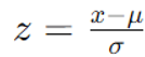
Where sigma σ is the standard deviation, μ is the feature mean, and x is the feature value.
When to Use:
a. Useful when features have different units or scales.
b. Commonly used with algorithms like K-Means, PCA, and hierarchical clustering.
2. Min-Max Scaling (Normalization)
Method: Rescale features to a fixed range, typically [0, 1].
Formula:
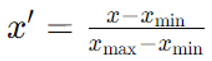
Where the values xmin, xmax, and x are the minimum and maximum of the original feature value, x.
When to Use:
a. Suitable for algorithms that assume data is bounded, like neural networks and some clustering algorithms.
b. Not ideal for data with outliers as it compresses the range of feature values.
3. Robust Scaling
Method: Scale features based on statistics that are robust to outliers.
Formula:
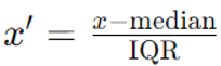
Where IQR is the Interquartile Range (75th percentile - 25th percentile).
When to Use:
a. Useful when data contains outliers.
b. Provides a more stable scaling compared to standardization when outliers are present.
4. MaxAbs Scaling
Method: Scale features by their maximum absolute value, transforming data to be in the range [-1, 1].
Formula:
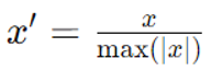
When to Use:
a. Suitable for sparse data (e.g., in text processing).
b. Preserves the sparsity of the data.
5. Log Transformation
Method: Apply a logarithmic transformation to reduce skewness in data.
Formula: x′=log(x+1)
Adding 1 prevents issues with taking the log of zero.
When to Use: Useful for data with exponential growth or highly skewed distributions.
6. Power Transformation
Method: To stabilize variance and improve the Gaussian appearance of the data, apply transformations such as the Box-Cox or Yeo-Johnson transformations.
Formula:
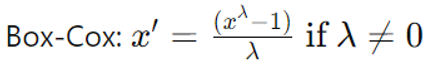
Yeo-Johnson: An extension of Box-Cox that works for both positive and negative values.
When to Use: Suitable for data that is not normally distributed and needs variance stabilization.
7. Quantile Transformation
Method: Features are transformed to have a normal or uniform distribution.
Formula: uses quantiles to map the features to a uniform or normal distribution.
When to Use: Useful for transforming data to a desired distribution, especially when the original data distribution is unknown or non-normal.
8. Unit Vector Scaling
Method: Scale each feature vector to have a unit norm.
Formula:
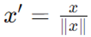
Where ∥x∥ is the norm of the vector.
When to Use: Ideal for cosine similarity-based techniques and K-Means algorithms, which are sensitive to the size of the feature vectors.
Choosing the Right Scaling Method
a. Understand Your Data: Consider the distribution, presence of outliers, and scale of your features.
b. Algorithm Requirements: Some clustering algorithms (e.g., K-Means) are sensitive to feature scales, while others (e.g., DBSCAN) are less so.
c. Domain Knowledge: Use domain expertise to select scaling methods that preserve the meaningful structure of your data. In addition to ensuring that each feature contributes to the clustering process in an acceptable manner, proper scaling can produce clustering results that are more accurate and useful.
Top of Form
3. Choosing the Right Algorithm
It depends on Algorithm Suitability and Algorithm Tuning.
Algorithm Suitability: Choose an algorithm that fits the nature of your data. For instance, K-Means assumes spherical clusters, while DBSCAN can handle clusters of arbitrary shapes.
Algorithm Tuning: Modify variables like the epsilon parameter in DBSCAN or the number of clusters in K-Means.
Algorithm Suitability
It is based on the Shapes of different clustering algorithms. Different clustering algorithms have different assumptions about the shapes and structures of clusters they can identify. Here’s a breakdown of various clustering algorithms and the types of cluster shapes they are best suited to detect:
1. K-Means Clustering
Shape: Spherical (Globular) Clusters
Details: K-Means makes the spherical, equal-size cluster assumption. By minimizing the variance within each cluster, it seeks to divide the data into k clusters. It functions best in compact, uniformly sized clusters.
Limitations: Struggles with non-spherical clusters, clusters with varying sizes, or clusters with different densities.
2. DBSCAN (Density-Based Spatial Clustering of Applications with Noise)
Shape: Arbitrary Shapes
Details: Based on the density of data points, DBSCAN finds clusters. Points in sparse regions are marked as noise, whereas points that are closely spaced together are grouped together. Clusters of any size and shape can be handled by it.
Limitations: Sensitive to the choice of parameters (epsilon and min_samples). May struggle with varying densities.
3. Hierarchical Clustering (Agglomerative and Divisive)
Shape: Arbitrary Shapes
Details: By dividing bigger clusters (divisive) or merging smaller clusters (agglomerative), hierarchical clustering creates a hierarchy of clusters. It can handle clusters of any shape and does not presuppose any particular cluster shape.
Limitations: Computationally intensive, especially for large datasets. May have difficulty with clusters of widely varying densities.
4. Gaussian Mixture Models (GMM)
Shape: Elliptical
Details: According to GMM, data points are produced by combining a number of Gaussian distributions with various covariances and means. It is most effective for elliptical-shaped clusters.
Limitations: Assumes that clusters follow Gaussian distributions, which may not be true for all data.
5. Mean Shift
Shape: Arbitrary Shapes
Details: Mean Shift identifies clusters by shifting a kernel (e.g., a Gaussian kernel) to the mode of the dataIt can handle clusters of any size and shape and doesn't assume any particular shape.
Limitations: Computationally expensive and requires choosing the bandwidth parameter carefully.
6. Spectral Clustering
Shape: Arbitrary Shapes
Details: Prior to using a clustering technique like K-Means, spectral clustering does dimensionality reduction using the eigenvalues of a similarity matrix. It is able to identify groups of intricate structures and forms.
Limitations: computationally demanding and maybe dependent on the selection of the similarity matrix.
7. Affinity Propagation
Shape: Arbitrary Shapes
Details: It is not necessary to predetermine the number of clusters when using affinity propagation. It can handle clusters of any shape and recognizes clusters based on messages passing between data points.
Limitations: It can be computationally intensive and sensitive to parameter settings.
8. BIRCH (Balanced Iterative Reducing and Clustering using Hierarchies)
Shape: Spherical and Some Arbitrary Shapes
Details: BIRCH builds a tree structure (CF tree) to summarize the data and performs clustering on the resulting clusters. It can handle clusters of varying sizes but assumes clusters are relatively spherical.
Limitations: May have difficulties with very irregular shapes.
9. OPTICS (Ordering Points to Identify the Clustering Structure)
Shape: Arbitrary Shapes
Details: OPTICS is an extension of DBSCAN that handles varying densities and creates a reachability plot to identify clusters of varying shapes and sizes.
Limitations: It can be complex to interpret and sensitive to parameter settings.
10. HDBSCAN (Hierarchical DBSCAN)
Shape: Arbitrary Shapes
Details: HDBSCAN extends DBSCAN by first building a hierarchy of clusters and then selecting the most appropriate clusters from this hierarchy. It can handle clusters of varying densities and shapes.
Limitations: Requires careful parameter tuning but is robust to noise and varying densities.
4. Dimensionality Reduction
It consists of three techniques. They were
a. Principal Component Analysis (PCA).
b. t-Distributed Stochastic Neighbor Embedding (t-SNE).
c. LDA (Linear Discriminant Analysis).
PCA (Principal Component Analysis): Reduce dimensionality to simplify the clustering problem while preserving variance [29].
t-SNE (t-Distributed Stochastic Neighbor Embedding): It is helpful for reducing dimensionality while maintaining local organization in the data (mostly used for visualization) or for showing high-dimensional data in 2D or 3D[30].
LDA (Linear Discriminant Analysis): It determines which linear combination of features best distinguishes between various classes.
5. Handling Noise and Outliers
Outlier Detection: Remove outliers that can skew clustering results.
Robust Algorithms: Use algorithms like DBSCAN that are less sensitive to noise and outliers.
6. Distance Measures
The distance metric used in clustering can have a big influence on the outcomes.
Commonly used distance metrics:
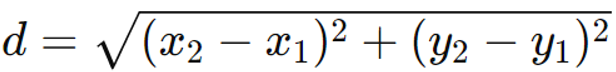
Euclidean Distance
Definition: The straight-line distance in Euclidean space between two places is measured as the Euclidean distance.
Formula: In a 2-dimensional space for points (x1,y1) and (x2,y2), Euclidean distance is given by:
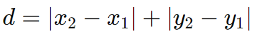
Manhattan Distance (L1 Norm)
Definition: The Manhattan distance, which is a grid-based method that quantifies the separation between two sites, such as city blocks, is sometimes referred to as the L1 distance or the taxicab distance. Because it approximates the distance a taxicab would travel on a grid of streets like Manhattan in New York City, it is known as the Manhattan distance.
Formula: In a two-dimensional space, for points (x1,y1) and (x2,y2), the Manhattan distance is given by:
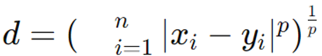
Minkowski Distance
Definition: A generalization of Manhattan distance and Euclidean distance is called Minkowski distance. It can be adjusted to accommodate different types of distance measurements depending on the value of a parameter p. This makes it a versatile metric for various applications.
Formula: In an n-dimensional space, for points (x1,x2,…,xn) and (y1,y2,…,yn),
the Minkowski distance d is defined as:
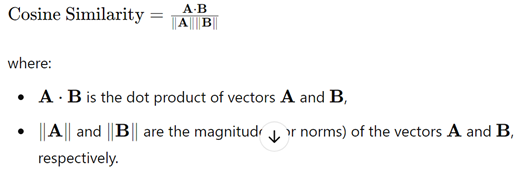
CosineDistance
Definition: A metric called cosine distance is used to compare and contrast two non-zero vectors, frequently in high-dimensional spaces, to ascertain how similar or unlike they are. It is frequently utilized in applications related to machine learning, information retrieval, and text analysis. Unlike distance metrics that rely on the magnitude of vectors, cosine distance focuses on the orientation or angle between vectors, making it useful for comparing the direction rather than the length.
Formula:
It is the
similarity between two vectors A and B is given by:
Jaccard Distance
Definition: It is a measure of dissimilarity between two sets. It is commonly used in fields like data mining, machine learning, and information retrieval, particularly when working with binary or categorical data.
Formula: For two sets A and B, the Jaccard similarity J is defined as:
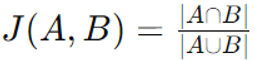
Where:
∣A∩B∣| is the number of elements in the intersection of A and B,
∣A∪B∣| is the number of elements in the union of A and B.
Hamming Distance
Definition: Hamming distance is a measure of the difference between two strings of equal length, representing the number of positions at which the corresponding symbols differ. It is particularly useful for tasks involving error detection and correction, as well as for comparing sequences or strings in various applications.
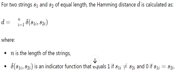
Formula:
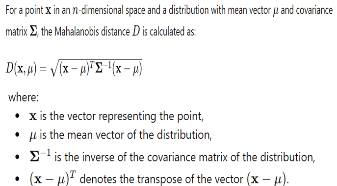
Mahalanobis Distance
Definition: The Mahalanobis distance quantifies the separation between a point and a distribution while taking the data set's correlations into account. Unlike Euclidean distance, which assumes all dimensions are uncorrelated and have the same scale, Mahalanobis distance accounts for correlations between variables and different scales of measurement. This makes it particularly useful in multivariate analysis.
Formula:
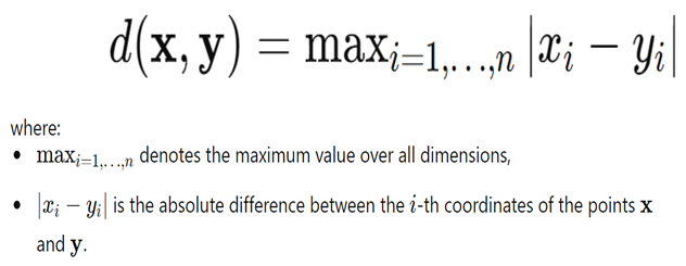
Chebyshev Distance
Definition: The greatest difference between the coordinates of two points in a space is called the Chebyshev distance, which is also referred to as the maximum metric or L∞ distance. It bears the name Pafnuty Chebyshev after the Russian mathematician.
Formula: For 2 points x=(x1,x2,…,xn) and y=(y1,y2,…,yn) in an n-dimensional space, the Chebyshev distance d is defined as:
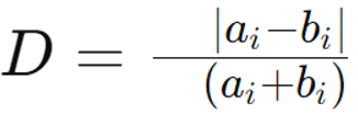
Canberra Distance
Definition: It is a metric used to measure the dissimilarity between two points in a space, especially useful in cases where the data can have varying scales or where some values are very small. It is sensitive to small values and can highlight relative differences between points. Canberra distance is often applied in fields such as ecology, bioinformatics, and data analysis.
Formula: For 2 points x=(x1, x2,…, xn) and y=(y1,y2,…,yn) in an n-dimensional space, the Canberra distance D is defined as:

Where x and y are points in the space, and xi and are the coordinates of the points in dimension i.
Bray-Curtis Distance
Definition: It is a metric used to quantify the dissimilarity between two samples based on their composition, commonly used in ecology and community ecology. It measures how different two samples are in terms of their abundance of various species or features.
Formula: The Bray-Curtis distance D between two samples A and B is given by:
Where
a. ai and bi are the abundances of the i-th species in samples A and B, respectively.
b. The numerator represents the sum of the absolute differences between the abundances of each species.
c. The denominator is the sum of the total abundances in both samples.
7. Cluster Evaluation and Validation [34]
Internal Validation: Use metrics like Silhouette Score, Davies-Bouldin Index, or Within-Cluster Sum of Squares to assess clustering quality.
External Validation: Compare clustering results to known labels using metrics like Adjusted Rand Index or Normalized Mutual Information.
8. Initialization Methods
Improved Initialization: For algorithms like K-Means, use methods like K-Means++ for better initialization of cluster centroids to avoid poor convergence [34].
9. Ensemble Methods
Cluster Ensembles: To increase accuracy and resilience, it combines the output of several clustering methods or iterations of the same algorithm[35].
10. Advanced Techniques
Hybrid Approaches: Combine different clustering methods or integrate clustering with supervised learning techniques for improved accuracy [36].
Deep Learning Approaches: Utilize neural network-based methods for clustering, such as autoencoders or deep clustering techniques [37].
11. Iterative Refinement
Re-clustering: Iteratively refine clusters by re-evaluating and adjusting parameters or features based on initial results. By systematically applying these methods and tuning them according to your specific dataset and goals, you can significantly improve the accuracy of your clustering results 38].
Confusion matrix
An essential tool in statistics and machine learning for assessing a classification model's performance is a confusion matrix. It offers a thorough analysis of the degree to which the model's predictions agree with the actual labels, including information about the different kinds of mistakes the model may have made [39].
Components of a Confusion Matrix
For a binary classification problem, a confusion matrix typically includes the following components:
True Positives (TP): How many times the positive class was accurately predicted by the model.
True Negatives (TN): The quantity of cases in which the model predicted the negative class with accuracy.
False Positives (FP): The quantity of cases where the model predicted the positive class erroneously—that is, when it predicted a positive class while the actual class was negative.
False Negatives (FN): The quantity of cases where the model predicted the negative class erroneously—that is, when it predicted a negative class while the actual class was positive. The Table 1 below depicts the organization of components of a 2x2 confusion matrix.
Metrics Derived from the Confusion Matrix
Several important performance metrics can be calculated from a confusion matrix:
1. Accuracy: the percentage of cases that were correctly classified out of all the instances.
Accuracy= (TP + TN) / (TP+TN+FP+FN)
2. Precision (Positive Predictive Value): the percentage of optimistic forecasts that come true.
Precision = TP / (TP+FP)
3. Recall (Sensitivity or True Positive Rate): the percentage of true positives that the model successfully detected.
Recall = TP / (TP+FN)
3. F1 Score: The precision and recall harmonic mean, which offers a single measure that strikes a compromise between the two issues.
F1 Score = 2* ((Precision *Recall)/( Precision + Recall))
4. Specificity (True Negative Rate): the percentage of real negatives that the model properly recognized.
Specificity = TN/ (TN+FP)
5. False Positive Rate: percentage of negatives that were mistakenly categorized as positives.
False Positive Rate = FP / (FP + TN)
6. False Negative Rate: the percentage of positive results that were mistakenly labeled as negative.
False Negative Rate = FN / (FN + TP)
II. Literature Survey
This survey consists of various Methods of feature selection & feature engineering methods. The right creation of the features is important to improve the accuracy and efficiency along with the feature selection. Table 2 depicts the feature selection methods and its sub methods. Table 3 show feature creation methods and its sub methods details.
Table 3: Details of feature Engineering methods and its sub methods
Research Gap
Combining the Feature selection & Feature Engineering to improve the accuracy of the model.
III PROPOSED ALGORITHM
The proposed algorithm is used to find the best features and apply Global Mean Based nearest Feature object Value Selection with Feature creation Method on it to improves the accuracy of the any clustering algorithm.
Algorithm steps
1. Take a data set. (Example iris data set).
2. Count the instances / records (X) present in the dataset as “N”.
3. Calculate the mean of all columns / features (Feature1_mean, Feature2_mean, ----, Featuren_mean)
4. Calculate the global mean from Individual means of all features of a dataset.
Feature1_mean= (Feature1_object1+ Feature1_object2+ ----+Feature1_objectn) /N
Feature2_mean =(Feature2_object1+ Feature2_object2+ ----+ Feature2_objectn)/N
And soon
Featuren_mean =(Featuren_object1 + Featuren_object2+ ----+Featuren_objectn)/N
Global mean = (Feature1_mean+ Feature2_mean+ ------ Featuren_mean)/N
5. Compute a feature (Global mean nearest value) using the Global mean nearest value method.
Nearest value= Value near to the Global mean for a instance or row of the data set
Nearest_value1= A value from one of the feature which is nearer to the Global mean for instance1 or Row 1(Feature1_object1, Feature2_object1, Feature3_object1, --------,Featuren_object1)
Nearest value2 = A value from one of the feature which is nearer to the Global mean for instance2 or Row2 (Feature1_object2, Feature2_object2, Feature3_object2, Featuren_object2)
And soon
Nearest valuen = A value from one of the feature which is nearer to the Global mean for instancen or Rown (Feature1_objectn, Feature2_objectn, Feature3_objectn, Featuren_objectn)
6. Choose a proper seed for the Kmeans Clustering Algorithm and apply on the data set.
7. Run the clustering Algorithm by selecting different combination of features.
Note:
1. The Best combination Features will give the best accuracy for the model along Global Mean Based nearest Feature object Value Selection with Feature creation Method.
2. The Table 4 below shows Global Mean Based nearest Feature object Value Selection with Feature creation Method reference table.
IV. Results
The results are generated by using python programming language using Anaconda Tool. The Table 5 depicts comparison of kmeans with, without along with Global Mean Based Nearest Feature object Selection, creation Method accuracy improvement.
V. Conclusions
Clustering is used to group the data. But the accuracy of the clustering always depends on the feature section and feature engineering methods. The Global Mean Based Nearest Feature objects Selection, creation Method with Kmeans with seed increase the accuracy of the model.
Author Contributions
Conceptualization, MDVP, ST; methodology, MDVP, ST; software, MDVP; validation, MDVP; formal analysis, ST; investigation, MDVP, ST; resources, MDVP, ST; data curation, MDVP; writing—original draft, MDVP; writing—review and editing, MDVP; visualization, MDVP, ST; supervision, ST; project administration, ST; funding acquisition, MDVP, ST. All authors have read and agreed to the published version of the manuscript.
Funding
No External or Internal Funding for this project.
Informed Consent Statement
There is no research with human subjects included in this article.
Data Availability Statement
No data sets were used or generated in this article.
Conflicts of Interest
The authors certify that they have no competing interests with relation to the work they have submitted.
Ethical considerations
Not applicable
References
- Maradana Durga Venkata Prasad, Dr. Srikanth T, “A Survey on Clustering Algorithms and their Constraints”, INTELLIGENT SYSTEMS AND APPLICATIONS IN ENGINEERING, 11(6s).
- Y. Singh and A. Mohan, “A Survey on Unsupervised Clustering Algorithm based on K-Means Clustering,” International Journal of Computer Applications, vol. 156, no. 8, pp. 6–9, Dec. 2016, doi: https://doi.org/10.5120/ijca2016912481. [CrossRef]
- D. Cao and B. Yang, “An improved k-medoids clustering algorithm,” Apr. 2010, doi: https://doi.org/10.1109/iccae.2010.5452085. [CrossRef]
- M. Roux, “A Comparative Study of Divisive and Agglomerative Hierarchical Clustering Algorithms,” Journal of Classification, vol. 35, no. 2, pp. 345–366, Jul. 2018, doi: https://doi.org/10.1007/s00357-018-9259-9. [CrossRef]
- D. Deng, “DBSCAN Clustering Algorithm Based on Density,” IEEE Xplore, Sep. 01, 2020.
- Patwary, D. Palsetia, A. Agrawal, W. Liao, F. Manne, and A. Choudhary, “Scalable parallel OPTICS data clustering using graph algorithmic techniques,” IEEE International Conference on High Performance Computing, Data, and Analytics, Nov. 2013, doi: https://doi.org/10.1145/2503210.2503255. [CrossRef]
- Y. Zhang et al., “Gaussian Mixture Model Clustering with Incomplete Data,” ACM Transactions on Multimedia Computing, Communications, and Applications, vol. 17, no. 1s, pp. 1–14, Jan. 2021, doi: https://doi.org/10.1145/3408318. [CrossRef]
- X. Wei and W. B. Croft, “LDA-based document models for ad-hoc retrieval,” Proceedings of the 29th annual international ACM SIGIR conference on Research and development in information retrieval - SIGIR ’06, 2006, doi: https://doi.org/10.1145/1148170.1148204. [CrossRef]
- W. Wang, J. Yang, and R. R. Muntz, “STING: A Statistical Information Grid Approach to Spatial Data Mining,” Very Large Data Bases, pp. 186–195, Aug. 1997.
- M. Rysz, Foad Mahdavi Pajouh, and E. L. Pasiliao, “Finding clique clusters with the highest betweenness centrality,” vol. 271, no. 1, pp. 155–164, Nov. 2018, doi: https://doi.org/10.1016/j.ejor.2018.05.006. [CrossRef]
- H. KUANG and J. LUO, “Text clustering based on genetic fuzzy C-means algorithm,” Journal of Computer Applications, vol. 29, no. 2, pp. 558–560, Apr. 2009, doi: https://doi.org/10.3724/sp.j.1087.2009.00558. [CrossRef]
- Y. Ng, M. I. Jordan, and Y. Weiss, “On Spectral Clustering: Analysis and an algorithm,” Neural Information Processing Systems, vol. 14, pp. 849–856, Jan. 2001.
- V. V. Mazur, K. A. Barmuta, S. S. Demin, E. A. Tikhomirov, and M. A. Bykovskiy, “Innovation Clusters: Advantages and Disadvantages,” DOAJ (DOAJ: Directory of Open Access Journals), Mar. 2016.
- Maradana Durga Venkata Prasad, Dr. Srikanth T, “Buddy System Based Alpha Numeric Weight Based Clustering Algorithm with User Threshold”, INTELLIGENT SYSTEMS AND APPLICATIONS IN , ENGINEERING, 12(8s).
- X. Zou, Y. Hu, Z. Tian and K. Shen, "Logistic Regression Model Optimization and Case Analysis," 2019 IEEE 7th International Conference on Computer Science and Network Technology (ICCSNT), Dalian, China, 2019, pp. 135-139, doi: 10.1109/ICCSNT47585.2019.8962457. [CrossRef]
- E. I. G. Nassara, E. Grall-Maës and M. Kharouf, "Linear Discriminant Analysis for Large-Scale Data: Application on Text and Image Data," 2016 15th IEEE International Conference on Machine Learning and Applications (ICMLA), Anaheim, CA, USA, 2016, pp. 961-964, doi: 10.1109/ICMLA.2016.0173. [CrossRef]
- Navada, A. N. Ansari, S. Patil and B. A. Sonkamble, "Overview of use of decision tree algorithms in machine learning," 2011 IEEE Control and System Graduate Research Colloquium, Shah Alam, Malaysia, 2011, pp. 37-42, doi: 10.1109/ICSGRC.2011.5991826. [CrossRef]
- J. K. Jaiswal and R. Samikannu, "Application of Random Forest Algorithm on Feature Subset Selection and Classification and Regression," 2017 World Congress on Computing and Communication Technologies (WCCCT), Tiruchirappalli, India, 2017, pp. 65-68, doi: 10.1109/WCCCT.2016.25. [CrossRef]
- N. Aziz, E. A. P. Akhir, I. A. Aziz, J. Jaafar, M. H. Hasan and A. N. C. Abas, "A Study on Gradient Boosting Algorithms for Development of AI Monitoring and Prediction Systems," 2020 International Conference on Computational Intelligence (ICCI), Bandar Seri Iskandar, Malaysia, 2020, pp. 11-16, doi: 10.1109/ICCI51257.2020.9247843. [CrossRef]
- M. A. Hearst, S. T. Dumais, E. Osuna, J. Platt and B. Scholkopf, "Support vector machines," in IEEE Intelligent Systems and their Applications, vol. 13, no. 4, pp. 18-28, July-Aug. 1998, doi: 10.1109/5254.708428. [CrossRef]
- E. Wilson and D. W. Tufts, "Multilayer perceptron design algorithm," Proceedings of IEEE Workshop on Neural Networks for Signal Processing, Ermioni, Greece, 1994, pp. 61-68, doi: 10.1109/NNSP.1994.366063. [CrossRef]
- R. Chauhan, K. K. Ghanshala and R. C. Joshi, "Convolutional Neural Network (CNN) for Image Detection and Recognition," 2018 First International Conference on Secure Cyber Computing and Communication (ICSCCC), Jalandhar, India, 2018, pp. 278-282, doi: 10.1109/ICSCCC.2018.8703316. [CrossRef]
- S. Zhang, F. Yang, D. Zhou and X. Zeng, "Bayesian Methods for the Yield Optimization of Analog and SRAM Circuits," 2020 25th Asia and South Pacific Design Automation Conference (ASP-DAC), Beijing, China, 2020, pp. 440-445, doi: 10.1109/ASP-DAC47756.2020.9045614. [CrossRef]
- K. Taunk, S. De, S. Verma and A. Swetapadma, "A Brief Review of Nearest Neighbor Algorithm for Learning and Classification," 2019 International Conference on Intelligent Computing and Control Systems (ICCS), Madurai, India, 2019, pp. 1255-1260, doi: 10.1109/ICCS45141.2019.9065747. [CrossRef]
- T. R. N and R. Gupta, "Feature Selection Techniques and its Importance in Machine Learning: A Survey," 2020 IEEE International Students' Conference on Electrical,Electronics and Computer Science (SCEECS), Bhopal, India, 2020, pp. 1-6, doi: 10.1109/SCEECS48394.2020.189. [CrossRef]
- J. Heaton, "An empirical analysis of feature engineering for predictive modeling," SoutheastCon 2016, Norfolk, VA, USA, 2016, pp. 1-6, doi: 10.1109/SECON.2016.7506650. [CrossRef]
- D. U. Ozsahin, M. Taiwo Mustapha, A. S. Mubarak, Z. Said Ameen and B. Uzun, "Impact of feature scaling on machine learning models for the diagnosis of diabetes," 2022 International Conference on Artificial Intelligence in Everything (AIE), Lefkosa, Cyprus, 2022, pp. 87-94, doi: 10.1109/AIE57029.2022.00024. [CrossRef]
- K. S. Prathyusha and B. E. Reddy, "Normalization Methods for Multiple Sources of Data," 2021 5th International Conference on Intelligent Computing and Control Systems (ICICCS), Madurai, India, 2021, pp. 1013-1019, doi: 10.1109/ICICCS51141.2021.9432142. [CrossRef]
- S. Naveen, A. Omkar, J. Goyal and R. Gaikwad, "Analysis of Principal Component Analysis Algorithm for Various Datasets," 2022 International Conference on Futuristic Technologies (INCOFT), Belgaum, India, 2022, pp. 1-7, doi: 10.1109/INCOFT55651.2022.10094448. [CrossRef]
- P. Hajibabaee, F. Pourkamali-Anaraki and M. A. Hariri-Ardebili, "An Empirical Evaluation of the t-SNE Algorithm for Data Visualization in Structural Engineering," 2021 20th IEEE International Conference on Machine Learning and Applications (ICMLA), Pasadena, CA, USA, 2021, pp. 1674-1680, doi: 10.1109/ICMLA52953.2021.00267. [CrossRef]
- E. I. G. Nassara, E. Grall-Maës and M. Kharouf, "Linear Discriminant Analysis for Large-Scale Data: Application on Text and Image Data," 2016 15th IEEE International Conference on Machine Learning and Applications (ICMLA), Anaheim, CA, USA, 2016, pp. 961-964, doi: 10.1109/ICMLA.2016.0173. [CrossRef]
- M. Mahin, M. J. Islam, A. Khatun and B. C. Debnath, "A Comparative Study of Distance Metric Learning to Find Sub-categories of Minority Class from Imbalance Data," 2018 International Conference on Innovation in Engineering and Technology (ICIET), Dhaka, Bangladesh, 2018, pp. 1-6, doi: 10.1109/CIET.2018.8660777. [CrossRef]
- G. Guo, L. Chen, Y. Ye and Q. Jiang, "Cluster Validation Method for Determining the Number of Clusters in Categorical Sequences," in IEEE Transactions on Neural Networks and Learning Systems, vol. 28, no. 12, pp. 2936-2948, Dec. 2017, doi: 10.1109/TNNLS.2016.2608354. [CrossRef]
- B. Çatalbaş, B. Çatalbaş and Ö. Morgül, "A new initialization method for artificial neural networks: Laplacian," 2018 26th Signal Processing and Communications Applications Conference (SIU), Izmir, Turkey, 2018, pp. 1-4, doi: 10.1109/SIU.2018.8404491. [CrossRef]
- D. Mienye and Y. Sun, "A Survey of Ensemble Learning: Concepts, Algorithms, Applications, and Prospects," in IEEE Access, vol. 10, pp. 99129-99149, 2022, doi: 10.1109/ACCESS.2022.3207287. [CrossRef]
- D. Yazdani, S. Golyari and M. R. Meybodi, "A new hybrid approach for data clustering," 2010 5th International Symposium on Telecommunications, Tehran, Iran, 2010, pp. 914-919, doi: 10.1109/ISTEL.2010.5734153. [CrossRef]
- Y. Guan, Y. Han and S. Liu, "Deep Learning Approaches for Image Classification Techniques," 2022 IEEE International Conference on Electrical Engineering, Big Data and Algorithms (EEBDA), Changchun, China, 2022, pp. 1132-1136, doi: 10.1109/EEBDA53927.2022.9744739. [CrossRef]
- Tian, L. Zhu, S. Zhang and L. Liu, "Improvement and parallelism of k-means clustering algorithm," in Tsinghua Science and Technology, vol. 10, no. 3, pp. 277-281, June 2005, doi: 10.1016/S1007-0214(05)70069-9. [CrossRef]
- S. Yaram, "Machine learning algorithms for document clustering and fraud detection," 2016 International Conference on Data Science and Engineering (ICDSE), Cochin, India, 2016, pp. 1-6, doi: 10.1109/ICDSE.2016.7823950. [CrossRef]
- M. Cherrington, F. Thabtah, J. Lu and Q. Xu, "Feature Selection: Filter Methods Performance Challenges," 2019 International Conference on Computer and Information Sciences (ICCIS), Sakaka, Saudi Arabia, 2019, pp. 1-4, doi: 10.1109/ICCISci.2019.8716478. [CrossRef]
- N. El Aboudi and L. Benhlima, "Review on wrapper feature selection approaches," 2016 International Conference on Engineering & MIS (ICEMIS), Agadir, Morocco, 2016, pp. 1-5, doi: 10.1109/ICEMIS.2016.7745366. [CrossRef]
- P. Gawade and S. Joshi, "Feature Selection for Embedded Media in the Context of Personification," 2020 Second International Conference on Inventive Research in Computing Applications (ICIRCA), Coimbatore, India, 2020, pp. 568-572, doi: 10.1109/ICIRCA48905.2020.9183293. [CrossRef]
- Kaur, K. Guleria and N. Kumar Trivedi, "Feature Selection in Machine Learning: Methods and Comparison," 2021 International Conference on Advance Computing and Innovative Technologies in Engineering (ICACITE), Greater Noida, India, 2021, pp. 789-795, doi: 10.1109/ICACITE51222.2021.9404623. [CrossRef]

Table 1.
Organization of components of a 2x2 confusion matrix.
| Predicted Positive | Predicted Negative | |
|---|---|---|
| Actual Positive | TP | FN |
| Actual Negative | FP | TN |
Table 2.
Methods of Feature selection and its sub methods.
| Feature Selection Methods | Sub Feature selection Methods | Sub Sub Feature selection Methods |
|---|---|---|
| Filter Method[40] | Statistical Tests | |
| Chi-Square Test | ||
| ANOVA (Analysis of Variance) | ||
| Mutual Information | ||
| Pearson Correlation Coefficient | ||
| Spearman’s Rank Correlation | ||
| Variance Threshold | ||
| Correlation Analysis | ||
| Wrapper Method[41] | Recursive Feature Elimination (RFE): | |
| RFE with Cross-Validation | ||
| Forward Selection | ||
| Backward Elimination | ||
| Bidirectional Elimination | ||
| Embedded Method[42] | Regularization Techniques | L1 Regularization (Lasso |
| L2 Regularization (Ridge): | ||
| Elastic Net | ||
| Tree-Based Methods | Decision Trees | |
| Random Forests | ||
| Gradient Boosting Machines (GBM) | ||
| Embedded Feature Selection Methods | LASSO Regression | |
| Embedded Feature Selection in Neural Networks | ||
| Feature Weighting in Linear Model | Feature Weighting in SVMs | |
| Linear Discriminant Analysis (LDA | ||
| Autoencoder-Based Feature Extraction | ||
| Feature Importance Analysis | Permutation Importance | |
| SHAP (SHapley Additive explanations |
Table 3.
Common Techniques for Feature Engineering.
| Methods of Feature Engineering | Sub Selection Method |
| Feature Engineering [43] | Domain Knowledge |
| Interaction Features | |
| Binning | |
| Dimensionality Reduction |
Table 4.
Global Mean Based nearest Feature object Value Selection with Feature creation Method.
| Feature1 | Feature2 | Feature3 | ---- | Featuren | Global mean nearest value |
|---|---|---|---|---|---|
| Feature1_object1 | Feature2_object1 | Feature3_object1 | Featuren_object1 | Nearest_value1 | |
| Feature1_object2 | Feature2_object2 | Feature3_object2 | Featuren_object2 | Nearest_value2 | |
| Feature1_object3 | Feature2_object3 | Feature3_object3 | Featuren_object3 | Nearest_value3 | |
| Feature1_objectn | Feature2_objectn | Feature3_objectn | Featuren_objectn | Nearest_valuen |
Table 5.
Results of Global Mean Based nearest Feature object Value Selection with Feature creation Method.
Table 5.
Results of Global Mean Based nearest Feature object Value Selection with Feature creation Method.
| Clustering Algorithm | Accuracy |
|---|---|
| Kmeans Without Seed | Output Varies |
| Kmeans With Best Seed | 0.96 |
| Global Mean Based Nearest Feature Object Selection, Creation Method With Kmeans With Best Seed | 0.9733333333333334 |
Author Details:
 |
Dr. SrikanthThota received his Ph.D in Computer Science Engineering for his research work in Collaborative Filtering based Recommender Systems from J.N.T.U, Kakinada. He received M.Tech. Degree in Computer Science and Technology from Andhra University. He is presently working as an Associate Professor in the department of Computer Science and Engineering, School of Technology, GITAM University, Visakhapatnam, Andhra Pradesh, India. His areas of interest include Machine learning, Artificial intelligence, Data Mining, Recommender Systems, Soft computing. |
 |
Mr. MaradanaDurgaVenkata Prasad received his B. TECH (Computer Science and Information Technology) in 2008 from JNTU, Hyderabad and M.Tech. (Software Engineering) in 2010 from Jawaharlal Nehru Technological University, Kakinada, He is a Research Scholar with Regd No: 1260316406 in the department of Computer Science and Engineering, Gandhi Institute of Technology and Management (GITAM) Visakhapatnam, Andhra Pradesh, INDIA. His Research interests include Clustering in Data Mining, Big Data Analytics, and Artificial Intelligence. He is currently working as an Assistant Professor in Department of Computer Science Engineering, CMR Institute of Technology, Ranga Reddy, India. |
Disclaimer/Publisher’s Note: The statements, opinions and data contained in all publications are solely those of the individual author(s) and contributor(s) and not of MDPI and/or the editor(s). MDPI and/or the editor(s) disclaim responsibility for any injury to people or property resulting from any ideas, methods, instructions or products referred to in the content. |
© 2024 by the authors. Licensee MDPI, Basel, Switzerland. This article is an open access article distributed under the terms and conditions of the Creative Commons Attribution (CC BY) license (http://creativecommons.org/licenses/by/4.0/).
Copyright: This open access article is published under a Creative Commons CC BY 4.0 license, which permit the free download, distribution, and reuse, provided that the author and preprint are cited in any reuse.


