
Submitted:
26 September 2024
Posted:
27 September 2024
You are already at the latest version
Abstract
Understanding the relationship between urban fabrics and sustainability is critical for addressing contemporary urban challenges. Urban fabrics contain information that reveals the performance and spatial heterogeneity of urban systems. This study evaluates the variability and spatial patterns of sustainability indicators across different urban fabric typologies in Cuenca, Ecuador. Using a 150-radius hexagonal grid covering the study area, 30 sustainability indicators are assessed in this study, exploring their spatial patterns and relationships with urban fabrics trough spatial and statistical analyses and visualization techniques. Results reveal significant variability among urban fabrics, with built environment indicators playing a dominant role in overall sustainability. There is evidence of marked spatial heterogeneity, with inner-core areas showing higher sustainability, while fringe expansion areas lag, and transitional areas also identified. Spatial clusters of high or low sustainability fabrics tend to be homogeneous, whereas mid-range sustainability fabrics exhibit greater heterogeneity. This quantitative evidence highlights hidden patterns in urban morphology and sustainability, offering valuable insights to support and enhance evidence-based urban planning. The open-source data and tools reported are developed to allow for customisation as well as replication in other urban areas.
Keywords:
sustainability indicators
; urban fabrics
; urban morphology
; intermediate cities
; GIS
; spatial analysis
1. Introduction
Urban sustainability is a widely recognised concept often adopted by planners, decision-makers, and politicians as a goal or characteristic of a given urban development model. It is commonly perceived as a quantitative measurement used to compare and rank cities as homogeneous entities. However, it is crucial to challenge this traditional understanding as cities are the product of complex evolutive processes, where different types of urban fabrics emerge, along with a mosaic of various typologies, each with its own formal and functional characteristics. These complex processes are evolutive by nature and have taken place over centuries of human and urban developments, hence, gazing upon cities’ evolution stands as an appropriate starting point.
The roots of land ownership and how it has influenced urbanism can be traced back to ancient times, from the circular house layouts of Natufian dwellings at Ain-Mallaha, 9000 BC, to orthogonal rooms or “Cell-building” at Cayonu, 8000 BC, to the emergence of street patterns in the city of Uruk, circa 3000 BC [1]. Street patterns in urban settlements became the boundaries between public and private property, kept in time by the politics derived from collective ownership [2]. The street is, therefore, the epicentre where human scale is experienced in a city, oscillating between public and private, architectural and urban scales. Several emerging city properties have their roots in the spatial configuration of the streets and buildings, such as the relation between pedestrian volumes and neighbourhood urban form or the imageability and complexity driving urban design features. Moreover, essential streetscape features influencing people’s lives are evidenced at the street level: historic buildings, outdoor dining, active uses, etc. [3]. Focusing on the street, the neighbourhood, on the human scale, stands as a fundamental premise for relevant urban analysis. Urban fabrics offer a great representation of such scales.
Urban fabric typologies can vary considerably around the globe, yet interesting similarities may exist for metropolitan areas, intermediate cities or smaller towns. This paper focuses on intermediate cities (100,000 to 500,000 inhabitants) and Cuenca, Ecuador, as a case study since these are argued to constitute the territories where most of the global urban population lives [4,5]. Intermediate cities are also vital within the “New Urban Agenda” established in Habitat III, being conceived as critical pieces for the achievement of the Sustainable Development Goals (SDG) [6].
Generally speaking, pursuing SDGs at the city level entails several challenges, such as data gathering, establishing indicators and metrics, monitoring, and implementation. Beyond the burden involved in data gathering efforts, a key consideration resides in measurement. A comprehensive measurement of cities’ sustainability should incorporate life-quality issues such as (dis)satisfaction with city life [7], urban imbalance and segregation [8,9], changing paradigms and policies [10], among others. Consequently, a methodological approach widely employed in urban contexts is creating urban sustainability indicators (USIs) [11], ranging from environmental and economic sustainability to equity and environmental justice at the city scale. Withal, SIs can be profoundly understood through what has been described as “strong sustainability” [12], which is focused on “increasing the efficiency of resource consumption; (ii) harvesting renewable resources limited by their regeneration rates; (iii) reducing greenhouse gas emissions; (iv) reusing wastes as input in other processes; (v) replacing toxic inputs with organic ones; (vi) replacing energy from non-renewable sources with that from renewable ones; (vii) increasing affordability; and (viii) increasing sustainable manufacturing” [12]. While urban research employing indicators has been conducted extensively on several domains in recent years, an over-attention to environmental aspects has been identified in the literature at the expense of socio-economic elements [13]. Moreover, the primary trend worldwide for measuring urban sustainability considers the city as a unique, homogenous body, computing aggregate city-wide indicators, thus disregarding spatial variability and the intrinsic heterogeneity of urban systems [14]. Cities are complex systems that result from adapting the natural environment to human conditions; as such, they display metabolic processes (production, consumption, and waste) analogous to the observable function of biological organisms within their ecosystems [15]. Managing cities as urban organisms in a sustainable and regenerative manner requires solutions that address the specific metabolic type of each city, seeking to “reduce its metabolic footprint (resource inputs and waste outputs) whilst improving its liveability” [11].
In line with the premise of considering streets, neighbourhoods and ultimately people, sustainable indicators must be applicable to a human scale, that is, to spatial units that a person can recognise and relate to in their daily life, ensuring that the metrics can ultimately be directed towards improving the quality of life of all inhabitants of a city [14]. Urban fabrics can be defined as confined city areas that present similar morphological characteristics, able to influence people’s experience and behaviour in aspects such as perception of space, commuting decisions, purchases and consumption, as well as the environmental performance of a place [16]. Urban fabrics have been classified by Wheeler [16] into 27 types of “built landscapes”, defined as an “area of consistent form at a neighbourhood scale, often 1 square km or greater. This is an area large enough to determine much of a resident or user’s daily experience and has a significant influence on shaping resident behaviour” ([16], p. 167). However, urban fabrics themselves cannot inform about sustainability, at least not directly or explicitly; hence, this paper aims to embed urban fabric typology data with a sustainability meaning. Connecting these two fundamental urban aspects can be instrumental in improving cities and their quality of life through urban planning. Additionally, the granularity implied in the urban fabric scale allows reaching the neighbourhood and citizen scale, thus addressing the limitations of USIs calculated at the aggregate city level, which would not capture cities’ heterogeneity adequately. Hence, this paper relies on a spatially disaggregate characterisation of USIs, whereby the study area is discretised by a spatial grid with observational units consisting of 150m-radius hexagons.
1.1. Related Literature
As a general comment on the broader literature, two of its key shortcomings have already been mentioned in the introduction: an over attention to environmental aspects of sustainability only, and a disregard to the need for a fine spatial disaggregation to capture the heterogeneity present at the human scale. In this context, this paper aims at establishing spatially-disaggregate, intra-city sustainability patterns within the urban area of Cuenca, characterizing and contrasting these findings according to an urban fabric typology of the city. While the literature review reported below relates to the focus of this paper from different angles, none of the branches and areas fully captures it, justifying the research gap identified. To the best of the authors’ knowledge, there is a dearth of literature mapping Urban Sustainability Indicators to an Urban Fabric Typology, hence, the literature review presented below mostly encompasses conceptual or methodological frameworks for urban sustainability indicators. Note that this paper does not aim at establishing conceptual frameworks for urban sustainability indicators or urban fabric typologies—rather, these are input data sources previously developed by the authors in earlier research efforts [17,18].
Four key aspects (search keywords) are considered to identify related literature: urban morphology, urban sustainability, GIS, and composite indicators (and variations of these keywords). Initial broad results are trimmed and narrowed based on relevance checks related to the scope of the paper and field of study (eliminating specific papers solely focused on water, energy, temperature, built environment, or the environmental dimension of sustainability, among others). A second selection criteria is based on manual inspection of paper titles, maintaining only those containing at least one of the four key aspects mentioned above. In a third stage, paper abstracts are inspected to assess relevance, which yielded 7 articles directly relevant to the aims and scope of this paper. Even though vitality, resilience, and sustainability cannot be considered equivalent (sustainability is a broader, more encompassing concept), 2 papers from these fields proposing indicators systems or frameworks are also added to the review, to draw some parallels.
In a study focused on resilience [19], a set of 42 indicators for the Madrid region are mapped to socio-cultural, economic, ecological, physical and technological, and governance system dimensions, yet at a high spatial aggregation at the level of municipalities, whereby the smallest unit is 5 km2, and the largest is 605.77 km2. Another study focused on urban vitality in Nanjing [20], a set of 71 indicators mapped to social, economic, cyberspace, and cultural-tourism dimensions, whereby a cellular automata grid of 500m rectangular blocks determines the level of spatial disaggregation.
As a transition from related fields to formal urban sustainability, a study first conducted in Australian cities and then expanded to other global cities addresses spatial indicators for urban liveability and sustainability that are oriented towards policy implementation [21]. Even though a formal distinction between liveability and sustainability is not clearly established, the reported definition of liveability is arguably quite close to sustainability. The approach employs a remarkably high spatial granularity, whereby indicators are calculated based on point data representations at the address level; nonetheless, it is also argued that grid cell data offers an effective mean to overcome the modifiable areal unit problem, as well as to enable scaling. Moreover, this study argues for establishing policy-relevant reference values for indicators, to provide standardized and comparable benchmarks, yet it is also acknowledged that these benchmarks are likely not universally agreed upon, or even representative of contexts and policy goals of different cities. In this context, it is worth mentioning that the broader research project to which this paper pertains does establish idealized optimal values based on assessments by local experts, as well as global standards from secondary sources. However, the main goal of this paper is a comparative examination of spatial patterns among urban fabrics, to establish interlinkages between urban sustainability and urban morphology. Such analyses would lack formality and would be obscured if true measurements were truncated to idealized optimal values (which, as argued above, can be subjective and context-dependent to a certain degree).
A study explicitly focused on urban sustainability is conducted in [22], yet with a high spatial granularity level set at Chinese cities/prefectures. Indicators are established at a single layer of 12 higher-level dimensions—as opposed most frameworks consisting of a lower layer of specific indicators mapped to an upper high-level layer of dimensions.
In a study of Spanish cities [23], the use of composite indicators to measure urban sustainability is also reported. The study strength lies in its representation of indicators by an interval from strong to weak sustainability, whereby the lower bound of the interval pertains to the worst performance (strong sustainability) and the upper bound pertains to the arithmetic mean (weak sustainability). The theoretical assumption behind strong sustainability implies that indicators aggregated into a composite global metric are non-compensatory (i.e., a good performance of one indicator does not make up for a poor performance in another), whereas weak sustainability implies perfect substitution (i.e., good performances of indicators balance out poor performances). A limitation of the study lies in its aggregate spatial granularity, as intra-urban heterogeneity among urban fabrics would be missed at the level of municipalities.
An illustrative contribution to the literature can be found in a review/conceptual framework assessing 67 indicator-led initiatives for urban sustainability, focusing on domains, themes, and suitability for different application purposes [24]. The paper identifies that the main domains targeted are, expectedly, the three fundamental pillars of sustainability: environment, society, and economy. Nevertheless, the study also identifies additional “irreducible” domains (higher-level layer) such as built environment, natural environment, governance, among others, and a wide variety of indicators (lower-level layer). These findings are postulated to demonstrate that consensus is yet to be achieved on semantics, classifications, and conceptual delimitations. In this context, the proposed approach in this paper relies on a comprehensive set of 30 indicators previously developed by the authors [24], which does not reduce sustainability to the three typical pillars and adopts a bottom-up structuring towards hierarchization: individual indicators mapped to four high-level dimensions (I: Built Environment, II: Biophysical Environment, III: Urban Systems, and IV: Socio-Spatial Integration). Contrasting against the characterization of domains and themes identified in [24], the indicator framework proposed in this paper covers most of them, while also establishing specific metrics for each indicator. Note that, while 58 indicators are originally defined in the research project to which this paper pertains, only 30 of them allowed for data collection in practice. Finally, the framework and set of indicators employed can be characterized as a theme-based approach according to the criteria established in [24], which is well aligned with purposes of structuring information and contextualizing metrics.
A GIS approach to identify relations between urban sustainability and urban morphology is proposed in [25]. The study reaches a sufficient granularity to capture human scale, as it employs a rectangular grid with spatial units that can reach 100x100m. Moreover, the study characterises urban sustainability by a hierarchical structure of 4 high-level dimensions (land occupation, public space and habitability, mobility and services, and urban complexity), mapped to 11 individual indicators (dwellings density, absolute compactness, corrected compactness, air quality, acoustic comfort, road accessibility, proximity of population to basic services, population movement mode, public road distribution, off-street parking, and balance between activity and residency). The study differentiates from the approach proposed in this paper in some respects. First, the set of indicators omits several aspects of urban sustainability: access to and extent of public space; non-automobile-based mobility seems to be neglected by solely defining road accessibility while off-street parking is an indicator on its own; access to and existence of green areas; access to basic services such as electricity or wastewater; and various types of socioeconomic and quality of life of the population (e.g., education level, quality of housing arrangements, unemployment, safety, residential location, etc.). In a subsequent study carried by the same authors [26], indicators measuring the degree of vacant urban lots and proximity to recycling are included. A second important difference consists of urban morphology being embedded and implicit in some built-environment indicators, yet an urban fabric typology is not explicitly considered, thus mapping sustainability and morphology is not pursued.
A contribution to the literature that relates to this paper to a higher degree is provided for the intermediate city of Mosquera-Colombia in [27], proposing an approach to measure urban sustainability through indicators, metrics and scoring. A spatial disaggregation to the level of neighbourhood is considered, albeit the study does not focus on the linkage to and characterization of sustainability levels with respect to urban fabric typologies. An argument is also made in [27] that sustainability assessment frameworks are lacking in three key aspects: granularity in their spatial disaggregation, approaching “all” sustainability dimensions (although the study adheres to the typical three “pillars”), and generalizability to other cities. has not approached “all” sustainability dimensions (although the study adheres to the typical three “pillars” of sustainability). In this sense, the approach proposed in this paper, the spatial units of analysis (hexagonal grid) and the set of sustainability indicators employed fully address the first two aspects. Regarding the third aspect, note that the main goal of this paper is aimed at establishing intra-city patterns and contrasts within the urban area of Cuenca as a case study, while inter-city comparisons with other urban areas fall outside of scope and are left for future work. Intra-city comparisons are particularly interesting due to the addition of an urban fabric typology layer, as it adds a key source of information that contributes to making meaningful distinctions of sustainability among different areas and fabrics of the city. Even though inter-city assessments are outside of scope, open-source tools are referenced later in this paper, which are expected to facilitate replication and application in other urban settlements.
The only study that closely matches the scope of this paper is proposed in [28], which first conducts an extensive literature review to identify frameworks for urban sustainability and typo-morphology, to then establish morphology characteristics at different scales (building, neighbourhood, block, and city), and sustainability dimensions (intensity, proximity, efficiency, accessibility, diversity, and permeability). While the study contemplates different scales, it does not characterize urban fabrics to the extent proposed by Wheeler [16]: in terms of the degree of differentiation or urban fabrics at the neighbourhood scale (limited to “buildings, plots, neighbourhood/local open space, local street system”); and regarding its level of spatial disaggregation (analysis units). Conversely, the approach proposed in this paper analyses a set of 30 urban sustainability indicators (also mapped to 4 high-level dimensions), against a typology of 18 distinct urban fabrics, at a fine level of spatial disaggregation.
In a nutshell, cities´ spatial (land distribution) and functional aspects (urban fabrics and population behaviour) are a source of considerable heterogeneity, which requires an appropriate scale to account for the differentiated flux of matter, energy, and waste of distinct parts of the city, and fully understand the urban metabolism of a city [14]. This approach is essential in the context of Latin American cities as well to reveal sustainability inequalities, considering that the region ranks as the most unequal in the world [29]. The contribution of this paper concerning the existing body of research in urban sustainability studies reported above consists of a first-of-its-kind assessment of the relationship among urban sustainability indicators and urban fabric typologies at a mesoscale (street and neighbourhood level of disaggregation, applied for city-wide analyses), taking the case study of the intermediate city of Cuenca, in the southern Andes region of Ecuador. This paper is interdisciplinary by nature, as it employs input data sources from urban morphology and urban sustainability, to then perform geographic and statistical analyses, connecting and enhancing both input fields. Among the main findings, evidence suggests that built environment indicators present significant variation among urban fabrics, dominating city-wide sustainability levels. A marked spatial heterogeneity is also revealed, with high-sustainability inner-core areas and low-sustainability fringe expansion areas, and in transition areas with mixed high/low sustainability. Sustainability of urban fabrics clusters is predominantly homogeneous for high/low sustainability levels, less homogeneous for urban fabrics clusters in the mid-range sustainability levels, and predominantly heterogeneous for transition areas. Implications and significance from these findings reside in their usefulness to urban planners and decision-makers, offering comparative insights and evidence on how sustainability varies among existing urban fabrics, which reveal otherwise hidden patterns implicit in plans and policies that have shaped current urban form and urban growth. These insights can enhance spatially-sensitive equity-based interventions and urban planning.
2. Data and Methods
This section describes the study area, the available input data for the analyses, and the statistical methods, visualisation techniques and GIS tools deployed for analyses.
2.1. Study Area
Cuenca is an intermediate city located in the southern Andes region of Ecuador at 2550 m.a.s.l.; its territory is geologically divided into three natural terraces marked by the Tomebamba and Yanuncay rivers. Founded by Spain in 1557, Cuenca´s urban layout followed the laws of the Indies and thus adopted the checkerboard grid still present in its downtown area. Since the 1950s, the city has experienced accelerated growth and currently is the third most populated city in Ecuador. Some key characteristics of the city are reported in Table 1 below.
As a newly induced Habitat III intermediate city, back in 2015, Cuenca embarked on a more robust pursuit of Sustainable Development Goals (SDG) [30], particularly SDG11: “Make cities and human settlements inclusive, safe, resilient and sustainable”. This unveiled an urgent need for a formal measurement of sustainability, encouraging diverse studies around the field for the city.
The city of Cuenca offers potential transferability within the region, as it displays a heterogeneous urban morphology representative of modern expansions of Latin American intermediate cities [17,31]. The authors have developed tools to facilitate transference and replication, which will be mentioned at the Discussion and Conclusion section of this paper.
2.2. Data
Following the argument supporting a vision of sustainability that addresses life-quality issues and metabolic processes of cities, a comprehensive set of indicators has been previously calculated for the city of Cuenca [17] under the assumption of a compact city model. The original set comprised 58 indicators at a conceptual level, yet full data exists for only 37 of them, and some additions have also been conducted for this study with respect to [17]. The updated set of indicators are grouped into four higher-level dimensions: I: Built Environment; II: Biophysical Environment; III: Urban Systems; and IV: Socio-Spatial Integration (Table 2). This set of indicators is the first key input data source enabling the analyses conducted in this paper and is stored in an open-access geographic information systems layer2, spatially disaggregated by a regular grid with hexagons of 150m radius.
A brief exploratory data analysis revealed that some USIs had all records either 100% (B1 and C13) or 0% (A7, A9, B3, C4, and C8). While these are extreme values with crucial practical significance, this study aims to assess differential patterns rather than overall sustainability magnitudes. Hence, these indicators are removed from consideration, leaving 30 USIs for analysis.
A second key input data source consists of a typology of urban fabrics, which has already been defined in previous research for the whole city of Cuenca [18], following the visual approach suggested by Wheeler [16] and adapting it to the local context. It is important to note that four rivers—Tomebamba, Tarqui, Yanuncay y Machángara—traverse the city and contribute to green areas of great importance; however, these typologies have been removed from the study since they do not represent populated areas and therefore, most indicators become irrelevant [18]. Eighteen UFTs result from the adaptation to Cuenca, each is briefly described in Table 3 and depicted in Figure 1; for a more detailed description see [18]. An open-access GIS layer3 with the identified UFTs is openly available as well.
The eighteenth type is labelled as UNCLASSIFIED, since these cells are located predominantly at expansion zones at the fringe of the study area, which can offer important insights regarding the sustainability of these zones.
An important instrument to enable analyses consists of urban fabric clusters, which can be defined as hexagonal cells of the same urban fabric type that are spatially agglomerated. These clusters delimited in Figure 1 by black boundaries and are established by leveraging QGIS4 geoprocessing tools by dissolving same-type cells sharing boundaries into a single geometry. Naturally, cases exist where only a few cells are found in proximity (even single isolated cells), hence, a minimum threshold of 7 cells is deemed adequate for cluster identification.
2.3. Methods
The approach proposed in this paper aims to explore relationships and patterns of urban sustainability indicators (USIs) with respect to urban fabric typologies (UFTs), which is achieved through data visualisation techniques, geospatial analyses, and statistical analyses. Both input data sources utilised (UFTs and USIs) are spatially disaggregated by the same 150m-radius hexagonal grid, granting a one-to-one mapping that eliminates the occurrence of spatial overlapping mismatches; the fine spatial disaggregation of the hexagonal grid employed also offers a workaround to avoid the modifiable areal unit problem as well as to allow for scalability [21,33].
2.3.1. Initial Statistical Tests
Two statistical tests are conducted at a pre-analysis step. First, 30 individual one-way ANOVA tests are conducted for each USI to assess whether there is a statistical variation of sustainability indicators for the 18 UFTs present in Cuenca. In other words, answering this question provides evidence that the means of each USI grouped by each UFT are significantly different among themselves. Note that spatial patterns are already considered implicitly in this analysis because, for every USI, the mean values of each UFT category correspond to averaging the values of all hexagonal cells of that category across the study area.
For the second pre-step, a Principal Component Analysis (PCA) is deemed necessary considering the high dimensionality involved in the study layout—having 30 USIs, each analysed against 18 UFTs. An important question to answer is whether each of the 30 USIs is pertinent in adding unique information and variability with respect to the rest. PCA is thus conducted to assess the degree to which the 30 USIs are correlated and whether it is pertinent to transform them into a lower dimensional array through linear transformations.
2.3.2. Statistical and Geospatial Methods
Due to the multidimensionality involved in this research layout (30 USIs contrasted against 18 UFTs), data analysis and visualisation require appropriate metrics and techniques, respectively. In the context, a fundamental step for enabling analyses consists of aggregating USIs into a composite sustainability index, which is computed as follows:
- Outliers for each USI are statistically treated first, based on the following criteria:
All values beyond the limits are truncated at the limit value.
- Then, each USI is normalised against its maximum value (upper limit, after truncation) in the [0, 1] domain. Note that this normalisation process is chosen instead of Z-scores, as centring values around zero would be inadequate for adding sustainability to all USIs.
-
The composite sustainability index consists of a linear combination (algebraic sum) of the 30 normalised USIs.
- o
- Note that some USIs are defined negatively regarding sustainability (e.g., unemployment). Hence, they enter the algebraic sum with a negative sign. The negative USIs are: A5, A10, D2, D3, D9, D11, D15, and D16. The logic is simple: Since they are negatively defined, the magnitude of a given negative USI (their ideal values being zero) reduces overall sustainability.
- o
- D17 is a particular case since its construction sets its optimal value as 1, and sustainability decreases both for values greater than 1 and lower than 1. Thus, the normalisation for this index consists of recentring it around zero (subtracting 1 from all values) and then converting negative values to absolute positive values. The normalised version of D17 measures a bidirectional distance from the optimal value.
It must be noted that the composite sustainability index’s purpose is to establish a common metric to enable formal comparison and differential analysis of sustainability patterns, among high-level sustainability dimensions and among different types of urban fabrics; hence, the index’s magnitude itself is not subject to analysis or interpretation in this study. This is also aligned with the rationale mentioned in Section 2.2 for removing USIs with all-100 or all-0 values.
Some indicator-based studies argue that individual indicators may capture more than one attribute and propose adding specific weight coefficients at the level of high-level dimensions [19]. In this sense, a useful application of the PCA pre-step mentioned above is assessing how well-differentiated (or not) USIs are regarding the information they provide, and thus deciding whether weighting is required.
Having computed the proposed composite index, several analyses can be conducted. First, a faceted boxplot of the composite index values can be leveraged to reveal intra- and inter-class patterns of each urban fabric typology. This visualisation offers simple, yet succinct, insights regarding how UFTs rank in terms of sustainability levels, but also on the variability present within each UFT.
To add statistical formality, an ANOVA test is conducted to contrast the composite sustainability index with UFTs, accompanied by Tukey’s Honest Significant Differences test, to test whether UFTs significantly differ among themselves, assessing pairwise combinations.
A natural question following the preceding analyses would focus on spatial patterns, arising questions such as, are there specific zones or areas in the city that display distinct composite sustainability levels? Or, whether patterns identified are linked to spatially clustered cells? These questions can be answered using geoprocessing techniques and methods, such as choropleth maps, and will also be addressed by data visualization techniques for high-dimensional data such as circular barplots5 and spider charts.
All spatial analyses presented in this paper are conducted in QGIS, while statistical analyses and visualisations are performed in R Statistical Software6.
3. Results
This section presents four main findings: first, the identification of statistically significant variability in Urban Sustainability Indicators (USIs) across different Urban Fabric Typologies (UFTs); second, evidence confirming the relevance and non-redundancy of the selected USIs; third, statistical analyses and visualization techniques that reveal both intra- and inter-class heterogeneity among UFTs in terms of sustainability levels; and finally, the detection of distinct spatial patterns of sustainability across the various UFTs trough choropleth maps and data visualizations.
3.1. One-Way ANOVA Tests
All 30 ANOVA tests were satisfactory, meaning that the null hypothesis of no statistically significant variation of each USI with respect to all UFT levels cannot be rejected. All tests yield p-values < 0.0001, implying high statistical significance. Results are shown in Table 4.
These tests offer first-order evidence justifying further analyses on the premise that statistically significant spatial heterogeneity exists in the data, considering the abovementioned argument that spatial patterns are implicit in the hexagonal spatial analysis units.
3.2. Principal Component Analysis
A different variable normalisation process is performed to conduct PCA, whereby USI variables are normalised as Z-scores—subtracting their mean and dividing by their standard deviation. A correlation plot is also helpful in gaining an initial perspective on the potential for dimensionality reduction. Figure 2 below suggests that correlation is generally low, with some variables showing an expected higher correlation due to their conceptual definition—e.g., A8-Proximity to open public spaces and B4-Proximity to green spaces.
PCA is then performed in R to identify principal components, which can be understood as linear transformations of the original USI variables. The next step consists of assessing the importance (relevance) of each principal component, which is achieved by creating a scree plot with the factoextra R package7. Figure 3 below shows the top 10 components in terms of the percentage of variance explained by them (all remaining 20 components explain less than 3% of variance each).
The results from the scree plot suggest that the linear transformations undertaken in the PCA procedure do not offer a justifiable reduction in dimensionality since the first principal component only captures 28% of the variance. The remaining components display an exponential decay pattern in variance explained, not even reaching 50% among the four best principal components.
All considered, evidence suggests that all USIs offer well-differentiated information, and it is best to maintain them in their original form; further, these results support constructing a composite sustainability index as a non-weighted linear combination of USIs (all with the same weight of 1), as the low correlation and high degree of differentiation aligns with an idealized hypothesis of perfect substitution (albeit not fully, naturally). Since the main goal of this paper is delivering a comparative examination of multicriteria sustainability among different types of urban fabrics, the proposed approach focuses entirely on pattern identification and statistical/spatial analyses, deliberately avoiding the use of weights or idealized optimal reference values, which can introduce subjectivity and context-dependency. Nonetheless, the establishment of weights and optimal values forms part of the broader research initiative to which this study contributes. Further details are available on the project’s website.8.
3.3. Composite Sustainability: Statistical Analyses
The results in Section 3.1 confirmed statistically significant variation of individual USIs among UFTs, but sustainability is an inherently complex multicriteria concept that cannot be reduced to one USI or another. In fact, this is a limitation of existing literature reported in Section 1.1, as literature commonly focuses on isolated aspects of urban morphology (e.g., built environment only) and/or urban sustainability (e.g., environment only). Variation must be assessed at the level of a composite sustainability index, as proposed in Section 2.3.2.
Building on this composite sustainability index, statistical analyses can be conducted to assess whether variability is significant at different levels. An ANOVA test assessing whether the composite sustainability index varies significantly with respect to UFTs yields an F-value of 86.32 and a significant p-value (≈0), thus, the null hypothesis of no statistically significant variation of the composite sustainability index with respect to all UFT levels cannot be rejected. This result complements and reconfirms results found at individual levels in Section 3.1.
Additionally, Tukey’s Honest Significant Differences test is conducted to assess significance at the level of UFT pairwise combinations. Results are shown in a matrix-table format in Table 5, generally showing that most pairwise combinations are statistically significant (A, N, O, and P only have 4, 4, 2, and 7 hexagonal cells, respectively). The null hypothesis of no statistically significant variation in the composite sustainability index between UFT pairwise combinations cannot be rejected. Results in Table 5 show that every UFT (except A, N, O, and P) is significantly different from, at least five other UFTs and, at most, nine. These results offer further proof that heterogeneity and significant differences in sustainability also exist among UFTs at more disaggregate levels.
3.4. Composite Sustainability: Data Visualisation and Analysis
Delving deeper into analyses, a more focused key question sought in this paper is: are some UFTs in Cuenca distinctly more sustainable than others? A first illuminating visualisation consists of boxplots depicting the distributions of composite sustainability indexes of each UFT, as shown in Figure 4 below.
Figure 4 displays boxplots of composite sustainability index in ascending order (read from left to right), clearly evidencing distinct sustainability levels among UFTs (inter-class variability), as well as considerable intra-class variation in several UFTs. While several contrasts can be made, the most interesting ones are arguably found at extreme values. Notably, the average composite sustainability index of the Rectangular Block Grid typology is around twice than the Allotment Gardens index (the comparison against Apartment Blocks is omitted due to scarce observations). Boxplots also convey important differences regarding intra-class variability, whereby UFTs with the highest variation are Upscale Enclave, Heavy Industry, and Garden Apartments. At the same time, the UTF with the lowest variation is Urban Grid (UFTs with a low number of observations cannot be considered when assessing intra-class variation). In other words, it can be stated that Urban Grid hexagonal cells are much more homogeneous in terms of their average composite sustainability index than the remaining UFTs.
Considering the results for UNCLASSIFIED shown in Figure 4, along with the results reported in Table 5, the inclusion of this UFT for analysis is fully justified, as these results collectively show a distinct pattern of low sustainability and significant variation with respect to most UFTs.
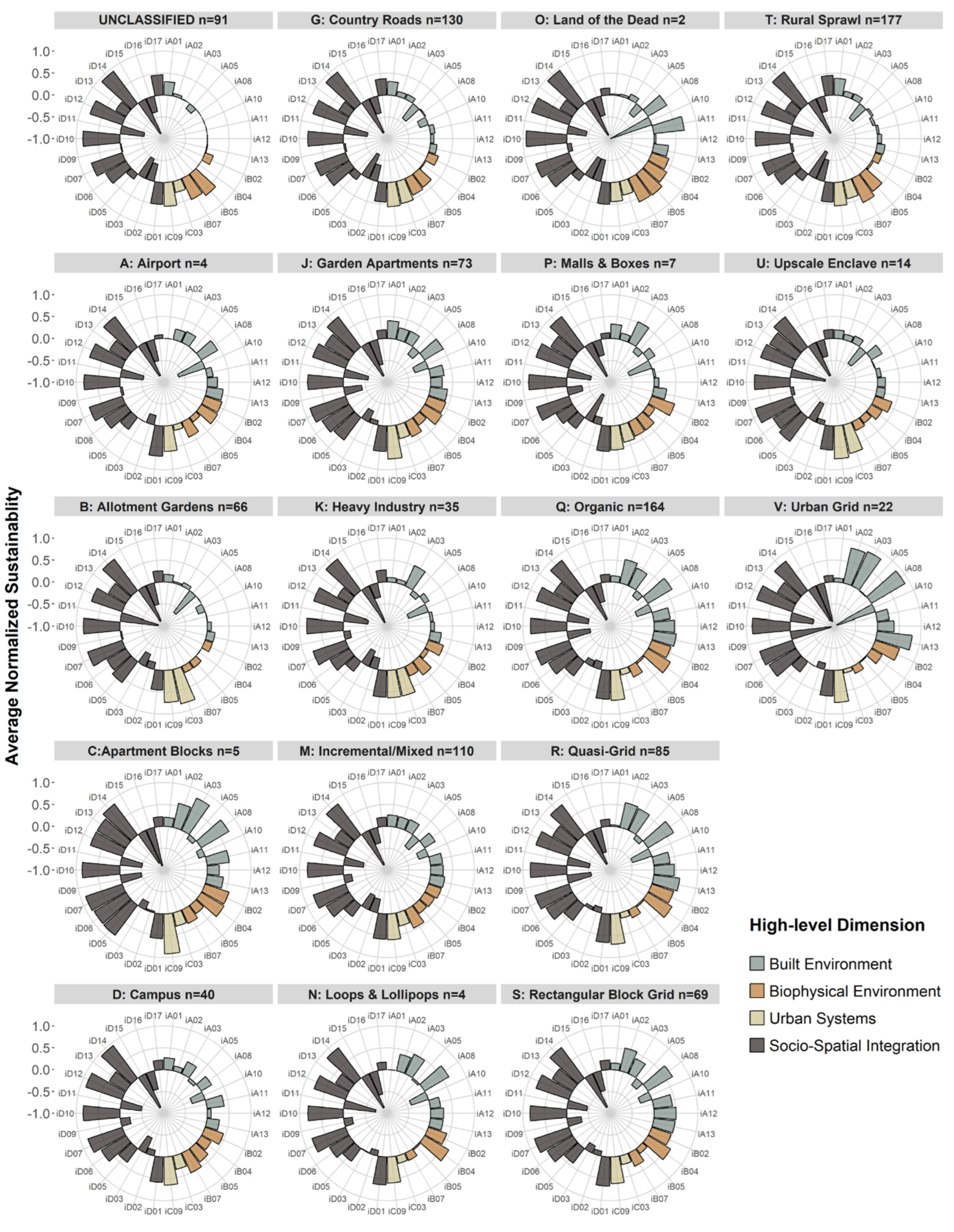
To complement the information provided thus far, a circular barplot is utilised next. It is worth mentioning that circular barplots are sometimes criticized since they can create visual distortion, as any bar representing a variable (UFT) is wider for higher values of that variable than for lower ones. Formally, the issue arises since one-dimensional variables are plotted as two-dimensional shapes, implying that a unitary value increase might appear visually smaller for low values, whereas larger for high values. To address this caveat, the bar width parameter in Figure 5 is reduced by 30% to approach rectangularity, and the plot ring corresponding to index=0 is offset by 3 units from the actual centre (as the above-mentioned distortion increases as the bar is closer to the circle centre). Conversely, the upside of a circular barplot resides in its ability to display and facet the information form several variables in a single condensed plot, facilitating comparative visualisation. Lastly, while a circular barplot relies on average points and does not inform about intra-class variations (unlike boxplots), it enables a clear visualisation of the comparative influence of high-level dimensions [34].
Prior to analysis, it is important to bear in mind the rationale argued in Section 3.2: weighting is not applied in this paper to avoid altering data and adopting arbitrary conventions regarding relative importance of indicators or dimensions (methodologically sound for practical purposes, but not suited for statistical and pattern analyses). The number of indicators (with field data available) in each dimension varies considerably (9, 4, 2, and 15, respectively), which implies that each dimension contributes in an unbalanced manner to the composite index. Nonetheless, at an individual USI level, it would be incorrect to artificially increase the contribution of two Urban Systems USIs while decreasing the contribution of fifteen Socio-Spatial Integration USIs; should D6_Use of time as an individual USI be disproportionately less impactful than C03_Public roads per inhabitant? Certainly not solely due to the circumstantial fact of a dimension having less indicators with available data.
All considered, Figure 5 reveals that, compared to other dimensions, Socio-Spatial Integration contributes rather homogeneously to composite sustainability among UFTs—but also evidencing clearly its overrepresentation. Conversely, a distinct, quite heterogeneous pattern among UFTs can be observed for Built Environment, which unveils a first strong piece of evidence suggesting that this dimension alone can largely explain composite sustainability patterns (i.e., ranking UFTs by composite index or by Built Environment would yield similar results, aside from V, M and N UFTs). While comparative variation can also be observed in Biophysical Environment, the pattern is not as marked, and differences are specific and intuitive (e.g., comparatively lower biophysical performance for Urban Grid while comparatively higher for Land of the Dead). The Urban Systems dimension is largely homogeneous among UFTs as well, notable exceptions where this dimension is comparatively higher are Allotment Gardens and Upscale Enclave.
Considering the high dimensionality involved in this paper (30 USIs by 18 UFTs), a visualization analysis focused on high/low-performing UFTs is deemed pertinent. To this end, a spider chart is shown in Figure 6, contrasting the three highest-sustainability UFTs (green-coloured polygons) versus the three lowest (pink-coloured polygons)—the choice of colours seeks contrast maximisation to facilitate analysis. The chart reports sustainability metrics for these six UFTs at a disaggregate level of individual USIs. Each spike of the plot maps the metric of a specific USI, whereby positively defined USIs values within the [0, 1] range are shown above the dashed inner circumference, and negatively defined USIs in the [0, -1] range are mapped below, towards the centre of the plot.
Note that the spider chart does not suffer from the caveat discussed earlier for circular barplots, since sustainability values are a simple dot along the axis of each USI, and polygons link these dots to provide an overall perspective of USIs performance for each UFT. Moreover, areas enclosed by the polygons are shaded to enhance the visualization of differences among UFTs.
Generically, a logical expectation would be that polygons of high-performing UFTs would encompass polygons of the low-performing USIs (applies for both positive and negative USIs). While this rationale holds for several USIs, some other USIs reveal interesting patterns.
First, in terms of USIs from the Socio-Spatial Integration dimension, low-performing UFTs score quite close to high-performing UFTs for most USIs, further supporting the interpretation of Figure 5 that the city performs quite homogenously among UFTs in this aspect. Accentuated differences where vertices of green polygons appear higher than pink polygons (following logical expectation) include D01_Households fully covered by basic services, D02_Household with critical construction deficiencies, D03_Dwellings at risk zones, D06_Use of time, and D13_Economically active population with university degree, this clearly suggests that differences can be attributed income segments of the population. Conversely, seemly counterintuitive patterns emerge whereby low-performing USIs far surpass high-performing ones, as evidenced in D09_Thefts per year and D17_Spatial segregation, however both cases can also be explained by income and quality of life conditions—thefts are much more likely to happen and spatial segregation to take place to and at high-income segments.
Second, USIs from the Urban Systems dimension do not show very clear patterns, as high- and low-performing UFTs are intertwined; for instance, in C09_Electricity consumption of households, Allotment Gardens (worst UFTs in composite sustainability) ranks second after Apartment Blocks (best composite). In the case of C03_Public roads per inhabitant, an opposite pattern was found, which, at first sight, would suggest that the most sustainable UFTs lack road networks. Assessing this indicator requires careful interpretation of extreme cases, as an insufficient road network would deteriorate both sustainable (e.g., public transit, bike) and unsustainable mobility (e.g., private vehicles), whereas cities where public space is disproportionately allocated to roads are the archetypical example of car-dependent unsustainability.
Third, USIs from Biophysical Environment show expected patterns. High-performing UFTs score considerably better than low-performing ones for B02_Nocturnal illumination of public streets and B04_Proximity to green spaces. Conversely, B05_Green area per inhabitant and B07_Soil permeability show an inverted pattern, which is clearly explained by the degree of urbanization, as low-performing UFTs are expected to be located in less urbanized areas—spatial analyses conducted in the next subsection provide evidence to support this argument.
Fourth, most Built Environment USIs are the ones where the largest differences can be identified and follow expected patterns of high-performing UFTs being above low-performing ones; this is strongly in line with the findings drawn from Figure 5 suggesting that most of the variability of the composite index is explained by the Built Environment dimension. Two exceptions emerge in this dimension: high- and low-performing UFTs are quite similar in terms of A_10 Relation between activity and residence, suggesting that mixed-uses are generally achieved to a good degree in urban fabrics of the city; and an inversion in A01_Net population density, indicating that UFTs that are ranked highest in overall composite sustainability are less dense in population than those ranked lowest. Again, the pattern found for A1 must be interpreted with some care to extreme cases, as high density can be sustainable in the context of compact self-contained mixed-use neighbourhoods, but it can also imply the presence of unsustainable features such as “conventillos”—a Spanish term referring to residential overcrowding. These results highlight the complexity of the concept of urban sustainability and the necessity of multi-dimensional approaches.
To complement statistical and visualization analyses, a more complex and detailed visualisation is provided in Appendix A, even though an assessment at the level of individual UFTs by individual USIs is not the aim of this paper. The visualization consists of a faceted circular barplot constructed at a fine granularity, simultaneously contrasting USIs, UFTs and high-level dimensions.
3.5. Spatial Analyses
The analyses conducted thus far have revealed statistically significant heterogeneity and distinct sustainability patterns among UFTs at different levels of aggregation —whether examined individually, by high-level dimensions, or through the composite index. In line with both the research objectives and practical urban planning needs, the next crucial step is to explore these patterns from a spatial perspective. A spatial perspective brings forth different types of questions, such as: are cells of UFT clusters homogeneous or heterogeneous in their composite sustainability indexes? Do certain areas or UFT clusters display distinctly high or low sustainability? Answering these questions is key to identifying spatial trends that could inform targeted urban interventions.
It is important to note that the following spatial analyses achieve a high level of disaggregation, i.e., 1098 hexagons of 150-m radius covering the urban area of Cuenca. However, certain urban fabric types—specifically A, C, N, O, P, U, and V —are represented by only a small number of hexagons. As a result, meaningful spatial patterns for these UFTs cannot be effectively identified due to their limited representation.
As a first step in addressing the aforementioned questions, Figure 7 presents a choropleth map of Cuenca spatially discretized by the hexagonal grid. A viridis colour scale characterises the range of values of composite sustainability indexes of cells, while the text labels overlaid on top of cells and cell clusters characterise urban fabric typologies.
A first assessment of Figure 7 is directed at complementing and further elaborating into the analyses of extreme values of sustainability. It can be evidenced that several urban fabric clusters have similar composite sustainability indexes indeed: for low-sustainability, B- and K- clusters at the northeastern boundary, K-clusters at the northern-central area, G- and T-clusters towards the north, and UNCLASSIFIED-, G- and T-clusters towards the south; whereas R-, Q- and S-clusters in the southern-central area, and a large Q-cluster towards the southwest, for high sustainability. This first finding would suggest considerable homogeneity in sustainability of urban clusters, at extreme sustainability levels.
A second relevant analysis focuses on mid-range sustainability values (the four blue-green hues in the centre of the viridis scale). Several areas with relatively homogeneous sustainability indexes can be identified in this case: a clearly defined V-cluster located at the Historic Centre of the city; a large J-cluster towards the south; R-, Q, and M-clusters at the southwestern end; B- and T-clusters at the western expansion area; Q, and M-clusters at the north-central area; and a D-cluster in the north-central area between the northern and northeastern expansion stripes. Homogeneity in mid ranges exists but it is less pronounced, even with a few single-cell outliers of higher sustainability emerging in some clusters.
Contrasting the patterns found thus far, several clusters can be identified with marked heterogeneity in their indexes: B-clusters also in the northeast but closer to the more urbanized area; Q-clusters in the central-northern area; R-clusters in the central area; J-, G-and M- clusters near the thin stripe connecting the northeast expansion with the urbanized core; M-clusters in the south; and UNCLASSIFIED-clusters at the northeastern and northwestern expansion stripes of the city. Interestingly, an S-cluster “oasis” of high sustainability can be located at the onset of the northern-central expansion area of the city, lying amid a very low sustainability area. The clusters identified in this analysis are considerably heterogeneous in their sustainability levels and can be considered as transitioning areas.
The analyses presented above leveraged urban fabric clusters as analysis units for exploring sustainability patterns of homogeneous morphological areas of the city. As a second step, the results from Figure 6 in Section 3.4 are complemented by addressing extreme sustainability levels from a spatial perspective. For this purpose, Figure 8 depicts the two highest versus the two lowest levels of sustainability from the composite index range, filtering out the four mid-ranges. The resulting image provides a marked pattern, evidencing complete spatial separation, with the sole exception of the “S-cluster oasis” identified earlier at the central-northern area of the city. High and low sustainability areas are mutually exclusive, which denotes unsustainable patterns at sprawling zones along the fringe of the city.
By complementarity, the greyed areas in Figure 8 represent mid-range sustainability, which in general are randomly scattered across the study area, except for two specific patterns. The first area without mid-range cells is the high sustainability Q-, R-, S-cluster in the southern-central area of the city, which encloses a considerable number of cells. Conversely, a second interesting pattern lies in the agglomeration of mid-range cells in expansion areas of the city towards the northeast, northwest and southwest, which may indicate that some smaller within expansion zones seem to be breaking the unsustainable trend at fringe areas identified earlier. Finally, a pattern worth mentioning can be observed in a “longitudinal chain” of high-sustainability J UFTs detaching from the central Q-, R-, S-cluster, which seems to be progressing towards and connecting with the north-eastern expansion stripe.
A final spatial analysis is conducted to complement the findings presented in Section 3.4 about sustainability patterns of high-level dimensions. Visualisation through a circular barplot showed that Built Environment patterns closely resemble composite sustainability patterns while Socio-Spatial Integration, Biophysical Environment and Urban Systems dimensions are largely homogeneous across UFTs, with some specific exceptions. However, some lingering questions remain regarding the spatial patterns of high-level dimensions: do the trends observed in data analyses hold spatially? Are there additional patterns and comparative insights when data is spatially laid out? To answer this question, USIs are partially aggregated at the level of each of their corresponding higher-level dimension to then generate choropleths. Analysing spatial patterns of sustainability at this level of aggregation (4 choropleths of high-level dimensions,) offers a balanced trade-off between full aggregation (1 choropleth of composite sustainability) and full disaggregation (30 choropleths of individual USIs).
Considering that aggregating USIs at high-level dimensions implies a different range of sustainability values for each dimension, a scale with a unified range encompassing all dimensions is necessary to guarantee an unbiased comparative standpoint. Moreover, the unified scale now shows negative values at its lower end, which simply means that negatively defined USIs outweigh their positively defined counterparts in some cells. Note that the unified range of sustainability values will be different from the one shown in previous figures, hence, index values are solely meant for comparison among dimensions and should not be compared directly to previous figures.
Figure 9 reports four choropleths showing spatial patterns of each dimension, laid out in a grid pattern to facilitate comparison. UFT labels have been removed to simplify visualisation, since the focus is not placed on UFT patterns anymore but on the differential influence of dimensions in the composite index, or on comparison among dimensions.
A simple inspection of Figure 9 confirms that the findings of Section 3.4 can be extended to the spatial aspect to a great degree. Clearly, the spatial patterns and heterogeneity observed in the choropleth of Dimension I strongly dominate the remaining (largely homogeneous) dimensions. Moreover, contrasting choropleths of Dimension I and composite sustainability (Figure 7) evidences that spatial patterns hold close resemblance (considering visual patterns only, and disregarding index ranges, as explained earlier).
Dimensions III and IV are largely homogeneous in in their spatial distribution across the city and their sustainability levels. Dimension II is also confirmed to be homogeneous to a lesser extent, but the most interesting pattern that can be evidenced is that the index is quite homogeneous for mid-range sustainability cells at the urban inner core, while a dramatic decrease is observed at northern and northeastern expansion stripes. This is a great example of how disaggregation can unveil true patterns that would otherwise remain hidden, as the heterogeneity identified for Dimension II through data visualisation and analysis (circular barplot in Figure 5) arises from aggregating (quite homogeneous) mid-range values of the inner core with low values of the expansion stripes (quite homogeneous as well).
Generally, the choropleths shown in Figure 9 clearly depict the marked differences that may exist among the inner more urbanized core and the fringe and expansion areas of the city, which reinforces the importance of making these distinctions and combining data visualization and statistical analyses with spatially disaggregate analyses.
4. Discussion and Conclusion
The results reported in Section 3 of this paper confirm its main hypothesis and highlight the spatial heterogeneity of sustainability within Cuenca, since they provide conclusive evidence that not only urban fabric typologies display distinct sustainability patterns in their spatial distribution but also display considerable—inter- and intra-class variability. Statistical tests demonstrate significant variability and differences, both at aggregate and disaggregate levels, while data visualisation and spatial analyses provide graphical aid to better comprehend the identified patterns. The statistical and spatial heterogeneity found in this paper suggests that urban fabric types significantly influence sustainability performance at the city level. In other words, urban sustainability, as measured by the proposed indicators, is strongly associated with urban form at the mesoscale.
Moreover, identified patterns provide an understanding of macro-level city sustainability computed from micro-level analysis units (cells capturing the neighbourhood scale). This is particularly important to overcome aggregation limitations in archetypal city-wide sustainability metrics. Urban fabrics with high or low sustainability levels tend to be more spatially homogeneous, meaning that sustainability patterns are more predictable in these areas. This is especially true for the inner-core areas (high sustainability) and the fringe or expansion areas (low sustainability), which suggests that the inner core of Cuenca conforms to characteristics such as the compact city model, mixed-uses, and proximity, whereas expansion areas indicate unsustainable urban sprawl [35]. This finding suggests that urban sustainability efforts could be targeted more efficiently in fringe areas where interventions might bring the most significant improvements toward higher sustainability. On the other hand, areas of mid-range sustainability exhibit much greater heterogeneity in their sustainability levels and do not relate to spatial agglomeration of UTFs compared to high and low sustainability areas. This result suggests that transition areas exist within the city with various types of spatially intertwined urban fabric typologies. While proximity and mixed-use patterns are desirable, transition areas may present challenges for sustainability planning. Streamlined generic solutions would likely be insufficient for these heterogeneous areas, instead, specifically tailored and adaptable urban planning strategies are recommended to improve sustainability levels across all UFTs involved.
Conclusive evidence indicates that B: Allotment Gardens, G: Country roads, and UNCLASSIFIED are the least sustainable UFTs, while C: Apartment Blocks, S: Rectangular Block Grid, and R: Quasi Grid UFTs are the most sustainable. The identification of distinct sustainability patterns linked to specific urban fabric types provides actionable insights for urban planners and decision-makers, as they can use this information to prioritize interventions based on the specific urban fabric type, thereby improving the sustainability of both high-density core areas and low-density expansion areas. The findings support the development of equity-based interventions, especially in fringe and transitional areas where sustainability performance lags.
Further, the analyses suggest that Dimension I: Built Environment is a strong differentiator since it explains overall sustainability variation on Cuenca to a high degree. This finding implies that built environment factors such as housing density, compactness, and proximity to basic services are the most heterogeneous across the city, playing a crucial role in determining the sustainability of urban fabrics. Urban planners should aim to bridge the gap on built environment indicators among different UFTs and the areas where the least sustainable ones are located. Designing and managing urban growth in this manner can help achieve better sustainability outcomes.
Among the most relevant limitations of this study, the authors would like to acknowledge the following aspects:
1) While extensive data gathering efforts were conducted in 2018, several indicators from the original set of 58 could not be gathered due to various constraints. Ideally, gathering data for additional indicators in Dimension II: Biophysical Environment and Dimension III: Urban Systems would result in a more balanced representation. Nonetheless, the reader s reminded of the rationale established earlier regarding weighting, which is deemed relevant for practice-oriented purposes, whereas this paper aims at establishing relations and identifying patterns among UFTs and USIs from unaltered data.
2) While the criteria for removing the four rivers traversing the city of Cuenca is justified in [18] due to being non-habitable, it arguably impacts sustainability values of Dimension II: Biophysical Environment. As this study focuses on the relationship between sustainability and urban fabric typologies, and most population-driven indicators would be null in the case of rivers, the reader is referred to the original dataset for further detail in this aspect.
3) Segmentation analyses of sustainability of individual or composite indicators with respect to transversal variables such as income [27], gender, age, mobility impediments, etc. would add interesting dimensions to this study. Nevertheless, an important consideration to bear in mind is the combinatorial challenge already implied in this research layout exploring patterns of 30 sustainability indicators with respect to 18 urban fabrics. Overlaying transversal dimensions on top of this layout would render a combinatorial explosion in terms of managing visualizations, interpretations and discussions. Finally, note that transversal factors such as income, gender or age are indirectly captured by USIs, particularly those of Dimension IV: Socio-Spatial Integration, while heterogeneity of the population is also indirectly captured by the high granularity employed in the 150-m-radus hexagonal grid.
Regarding future work, the authors would like to mention the following avenues:
1) Addressing the data availability limitations discussed above, aiming for periodical data gathering to allow for monitoring and longitudinal analyses. However, an important challenge exists in data gathering efforts for such an extensive set of indicators (58 considering the complete set), and at a high level of disaggregation (150-m-radius hexagons), as it can be quite resource-intensive. Ideally, collaborating between academia and the public sector would confer economic feasibility and project sustainability over time. Also, while the study revealed critical patterns, certain sustainability indicators had extreme values (either 100% or 0%), which may not fully reflect the variability needed for deeper analysis in some dimensions, such as Biophysical Environment. Future work should aim to collect additional data to balance the representation across all sustainability dimensions.
2) The exclusion of river areas from the study also presents a limitation, particularly in terms of their impact on the Biophysical Environment dimension. Future research could integrate the proximity to these areas to better capture their effect on urban sustainability.
3) Segmentation analyses can certainly be conducted in future work, shifting the focus from pattern identification. Reducing dimensionality in the research layout would be essential in this case, potentially by relying solely on the composite index or high-level dimensions. Moreover, assigning weights to indicators and balancing the number of indicators among high-level dimensions would be recommended for segmentation analyses, as the aim would shift from data analyses to a more practice-, policy-oriented population focus.
4) In addition to addressing limitations, future work is planned on pursuing a more complex methodological approach by employing econometric models in the branch of logistic regression, which would adjust well to the categorical-quantitative nature of the data (UFTs-USIs), and they would allow to further explore relations and effects among UFTs and USIs at a fully disaggregate level. An estimated logistic model could also be applied for elasticity analyses to assess the effect of changes in metrics (increased/decreased performance of USIs) on sustainability, as well as for predictive and labelling purposes.
5) In terms of flexibility, and to address some of the limitations as well as future work, it is worth mentioning that LlactaLAB has developed an open-access tool available as a QGIS complement named MESUE9, which offers specific functionality for exploring and customising different weightings in the construction of a composite index, as well as establishing of policy-oriented optimal values for indicators. Moreover, a second open-source, open-access tool developed consists of a QGIS toolbox plugin labelled SISURBANO10, offering automated tools to calculate a wide array of urban sustainability indicators from standardized input data in QGIS or CSV format. These tools can be utilised as a “sandbox” for customisation and exploration purposes that can range from conceptual and methodological, practical scenario analyses, or to test the methodological approach in other urban areas. This is an exciting research avenue, particularly for intermediate cities in the Andes and Latin America, to identify insightful similarities and differences.
The contributions of this paper are novel in terms of the level of disaggregation achieved, the comprehensiveness of the set of USIs, and, more importantly, since UTFs evolve from purely morphological characterisation of to incorporate a sustainability meaning. Findings from this paper also bring forth new questions regarding the drivers behind spatial and data patterns. Urban planners should consider spatial heterogeneity when designing policy interventions, particularly in the transition zones with mixed sustainability. Policies aimed at enhancing the sustainability of low-performing areas, such as the fringe expansion zones, could be prioritized for long-term urban sustainability strategies. Future research could include longitudinal analyses to track the evolution of urban fabric sustainability over time, allowing for more dynamic and predictive urban planning. Incorporating econometric models and other statistical tools could further explore the relationships between sustainability indicators and urban fabric typologies, providing deeper insights into the drivers of sustainability at both local and city-wide scales.
Author Contributions
Conceptualization, writing—original draft preparation, Francisco Calderón, Daniel Orellana, Maria Isabel Carrasco and Maria Augusta Hermida; methodology and investigation, Francisco Calderón, Daniel Orellana, Maria Isabel Carrasco, Johnatan Astudillo, and Maria Augusta Hermida; software, Johnatan Astudillo and Francisco Calderón; formal analysis, data curation, and visualisation, Francisco Calderón; writing—review and editing, Francisco Calderón and Daniel Orellana; supervision, project administration, funding, and funding acquisition, Daniel Orellana and Maria Augusta Hermida. All authors have read and agreed to the published version of the manuscript.
Funding
This research is part of the project “Evaluación de sustentabilidad en tejidos urbanos: Sistema de Indicadores y herramienta de análisis espacial (SISURBANO)“, funded by Dirección de Investigación de la Universidad de Cuenca. The APC was funded by Vicerrectorado de Investigación de la Universidad de Cuenca.
Data Availability Statement
The original data presented in the study are openly available at the GeoLlactaLAB web repository: http://201.159.223.152.
Acknowledgments
We would like to express our gratitude to the institutions that facilitated the access to the data for this research, including the GAD Municipal de Cuenca, Municipal Corporation, ETAPA, EMOV-EP, and Empresa Eléctrica Centro Sur. We are also grateful to technicians and experts who provided insights and feedback on the conceptualisation of sustainability indicators. Finally, we want to recognise the efforts of researchers at LlactaLAB UCuenca, in particular to research assistants and undergrad students who participated in the data collection and processing.
Conflicts of Interest
The authors declare no conflicts of interest. The funders had no role in the design of the study; in the collection, analyses, or interpretation of data; in the writing of the manuscript; or in the decision to publish the results.
Appendix A
Figure A1.
Normalised USIs, characterised by high-level dimension, and faceted by UFT.
| 1 | ECUADOR NATIONAL CENSUS 2022: https://www.censoecuador.gob.ec/resultados-censo/. |
| 2 | GeoLlactaLAB: Geonode LlactaLAB; http://201.159.223.152/layers/geonode_data:geonode:CompletoIndicad. |
| 3 | GeoLlactaLAB: Geonode LlactaLAB; http://201.159.223.152/layers/geonode_data:geonode:CompletoIndicad. |
| 4 | QGIS: https://www.qgis.org/. |
| 5 |
ggradar R package: https://r-graph-gallery.com/web-radar-chart-with-R.html. |
| 6 | R Statistical Software: https://www.r-project.org/. |
| 7 |
factoextra R package: https://rpkgs.datanovia.com/factoextra/index.html. |
| 8 | LlactaLAB: Ciudades Sustentables official website: https://llactalab.ucuenca.edu.ec/sisurbano/. |
| 9 | Modelo de Evaluación de Sustentabilidad Urbana Espacial – MESUE: https://github.com/llactalab/mesue. |
| 10 | LlactaLAB: Ciudades Sustentables official website – SISURBANO: https://llactalab.ucuenca.edu.ec/sisurbano/. |
References
- Aureli, P.; Turan, N. [Re]Form: New Investigations in Urban Form, Panel 1. Harvard GSD 2018. https://youtu.be/0L7Anlsu2A4.
- Doug Allen Institute. Streets Lecture—Part 1 2016. https://www.youtube.com/watch?v=NA2jpARqS7A&feature=youtu.be.
- Park, K.; Ewing, R.; Sabouri, S.; & Larsen, J. Street life and the built environment in an auto-oriented US region. Cities 2019, 88, 243–251. [CrossRef]
- González, L.G.; Siavichay, E.; Espinoza, J.L. Impact of EV fast charging stations on the power distribution network of a Latin American intermediate city. Renewable and Sustainable Energy Reviews 2019, 107, 309–318. [CrossRef]
- Mackay, H. Mapping and characterising the urban agricultural landscape of two intermediate-sized Ghanaian cities. Land Use Policy 2018, 70, 182–197. [CrossRef]
- United Nations. The New Urban Agenda. United Nations: Quito, Ecuador 2017; ISBN 978-92-1-132731-1.
- Valente, R.; Berry, B. Dissatisfaction with city life? Latin America revisited. Cities 2016, 50, 62-67. [CrossRef]
- Garcia-Ayllon, S. Rapid development as a factor of imbalance in urban growth of cities in Latin America: A perspective based on territorial indicators. Habitat International 2016, 58, 127–142. [CrossRef]
- Smets, P.; Salman, T. The multi-layered-ness of urban segregation. On the simultaneous inclusion and exclusion in Latin American cities. Habitat International 2016, 54, 80–87. [CrossRef]
- van Lindert, P. Rethinking urban development in Latin America: A review of changing paradigms and policies. Habitat International 2016, 54, pp. 253-264. [CrossRef]
- Thomson, G.; Newman, P. Urban fabrics and urban metabolism—from sustainable to regenerative cities. Resources, Conservation and Recycling 2018, 132, 218–229. [CrossRef]
- De Oliveira Neto, G.; Pinto, L.; Giannetti, A.; de Almeida, C. A framework of actions for strong sustainability. Journal of Cleaner Production 2018, 196, pp. 1629-1643. [CrossRef]
- Sharifi, A. Urban sustainability assessment: An overview and bibliometric analysis. Ecological Indicators 2021, 121. [CrossRef]
- Verma, P.; Raghubanshi, A. Urban sustainability indicators: Challenges and opportunities. Ecological Indicators 2018, 93, pp. 282-291. [CrossRef]
- Rojas, F.; Borthagaray, A.; Marques, A.; Chong, J.; Strobel, J.; Bonilla, L.; Mondino, M.; Pineda, M.; Ellinger, P.; Carrasco, P.; Nemirovsky, Y. La ciudad como sistema: metabolismo, resiliencia y sustentabilidad. Ediciones Irradia. Disruptiva. 2023; 1ª ed, ISBN 978-987-48044-3-3.
- Wheeler, S. Built Landscapes of Metropolitan Regions: An International Typology. Journal of the American Planning Association 2015, 81, 167–190. [CrossRef]
- Hermida, M.; Calle, C.; Cabrera, N. La ciudad empieza aquí: metodología para la construcción de barrios compactos sustentables. Universidad de Cuenca: Cuenca, Ecuador 2015, ISBN 978-9978-14-318-6.
- Hermida, M.; Cobo, D.; Neira, C. Challenges and Opportunities of Urban Fabrics for Sustainable Planning In Cuenca (Ecuador). IOP Conference Series: Earth and Environmental Science 2019, 290. [CrossRef]
- Suárez, M.; Benayas, J.; Justel, A.; Sisto, R.; Montes, C.; Sanz-Casado, E. A holistic index-based framework to assess urban resilience: Application to the Madrid Region, Spain. Ecological Indicators 2024, 166. [CrossRef]
- Wang, Z.; Wang; X.; Liu, Y.; Zhu, L. Identification of 71 factors influencing urban vitality and examination of their spatial dependence: A comprehensive validation applying multiple machine-learning models. Sustainable Cities and Society 2024, 108. [CrossRef]
- Higgs, C.; Alderton, A.; Rozek, J.; Adlakha, D.; Badland, H.; Boeing, G.; … Giles-Corti, B. Policy-Relevant Spatial Indicators of Urban Liveability And Sustainability: Scaling From Local to Global. Urban Policy and Research 2022, 40(4), 321–334. [CrossRef]
- Wang, C.; Quan, Y.; Li, X.; Yan, Y.; Zhang, J.; Song, W.; Lu, J.; Wu, G. Characterizing and analyzing the sustainability and potential of China’s cities over the past three decades. Ecological Indicators 2022, 136. [CrossRef]
- Lo-Iacono-Ferreira, V.; Garcia-Bernabeu, A.; Hilario-Caballero, A.; & Torregrosa-López, J. Measuring urban sustainability performance through composite indicators for Spanish cities. Journal of Cleaner Production 2022, 359. [CrossRef]
- Halla, P.; Merino-Saum, A. Conceptual frameworks in indicator-based assessments of urban sustainability—An analysis based on 67 initiatives. Sustainable Development, 30(5), 1056–1071. [CrossRef]
- Jiménez-Espada, M.; García, F.M.M.; González-Escobar, R. Urban Equity as a Challenge for the Southern Europe Historic Cities: Sustainability-Urban Morphology Interrelation through GIS Tools. Land 2022, 11, 1929. [CrossRef]
- Jiménez-Espada, M.; Martínez García, F.M.; González-Escobar, R. Sustainability Indicators and GIS as Land-Use Planning Instrument Tools for Urban Model Assessment. ISPRS International Journal of Geo-Information 2023, 12, 42. [CrossRef]
- Jorge-Ortiz, A.; Braulio-Gonzalo, M.; Bovea, M.D. Assessing urban sustainability: a proposal for indicators, metrics and scoring—a case study in Colombia. Environment, Development and Sustainability 2023, 25, 11789–11822. [CrossRef]
- Mobaraki, A.; Oktay Vehbi, B. A Conceptual Model for Assessing the Relationship between Urban Morphology and Sustainable Urban Form. Sustainability 2022, 14, 2884. [CrossRef]
- Programa de las Naciones Unidas para los Asentamientos Humanos. Construcción de Ciudades más Equitativas, Políticas públicas para la inclusión en América Latina. United Nations: Nairobi, Kenia 2014, ISBN 978-92-1-132605-5.
- United Nations Cuenca Declaration for Habitat III “Intermediate Cities: Urban Growth and Renewal”. Available online: http://habitat3.org/wp-content/uploads/Declaration-Cuenca.pdf (accessed on Oct 17, 2019).
- Cabrera, N.; Hermida, M., Orellana, D., Osorio, P. Assessing the sustainability of urban density. Indicators in the case of Cuenca (Ecuador). Bitácora Urbano Territorial 2015, 25(2). [CrossRef]
- Shannon, C; Weaver, W. The mathematical theory of communication. The University of Illinois Press—Urbana 1964, 14, pp. 306–317. https://www.ncbi.nlm.nih.gov/pubmed/9230594.
- Openshaw, Stan. The modifiable areal unit problem. Norwick: Geo Books 1983. ISBN 0860941345. OCLC 12052482.
- Burch, M.; Weiskopf, D. On the Benefits and Drawbacks of Radial Diagrams. Handbook of Human Centric Visualization 2014, pp.429-451. 1st ed. Springer; New York, NY, USA. ISBN 978-3-540-30750-1.
- Shawly, H. Evaluating Compact City Model Implementation as a Sustainable Urban Development Tool to Control Urban Sprawl in the City of Jeddah. Sustainability 2022, 14, 13218. [CrossRef]
Figure 1.
Eighteen urban fabrics within the metropolitan area of the city of Cuenca.
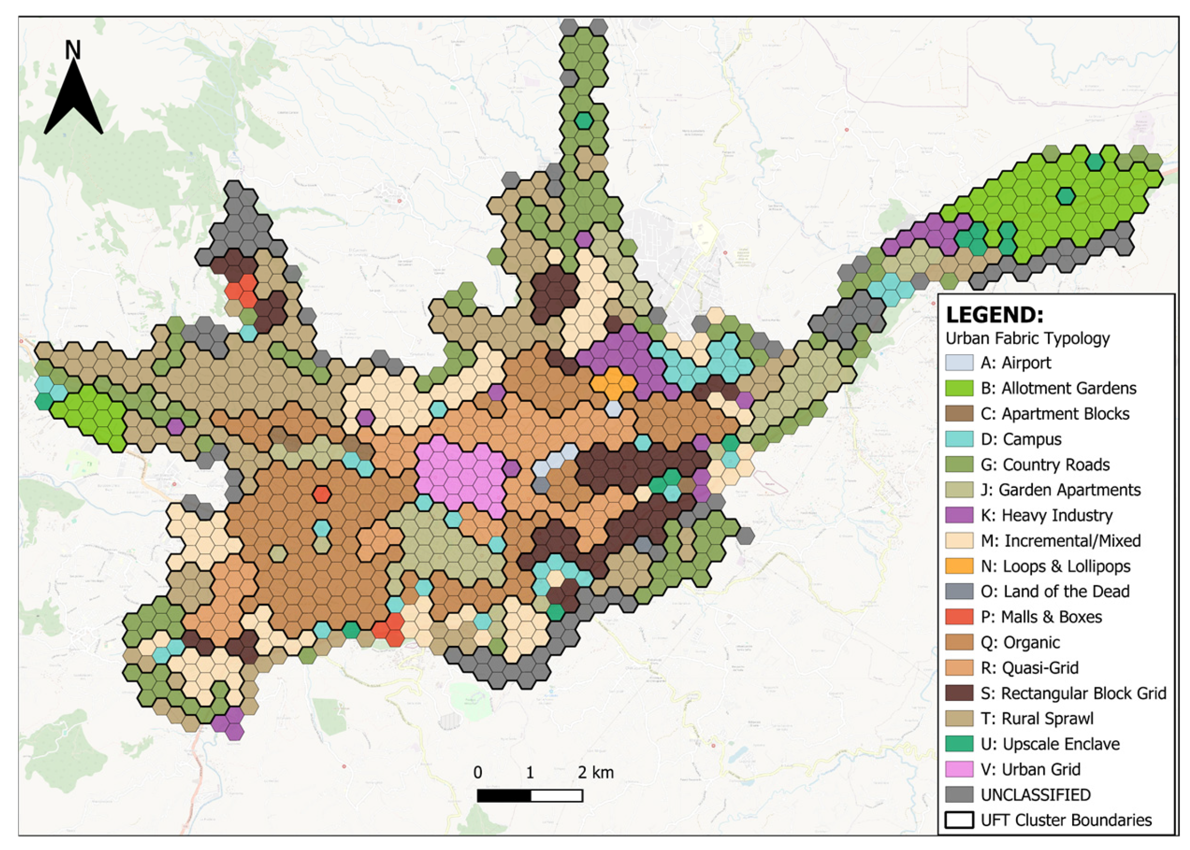
Figure 2.
Correlation plot among USIs.
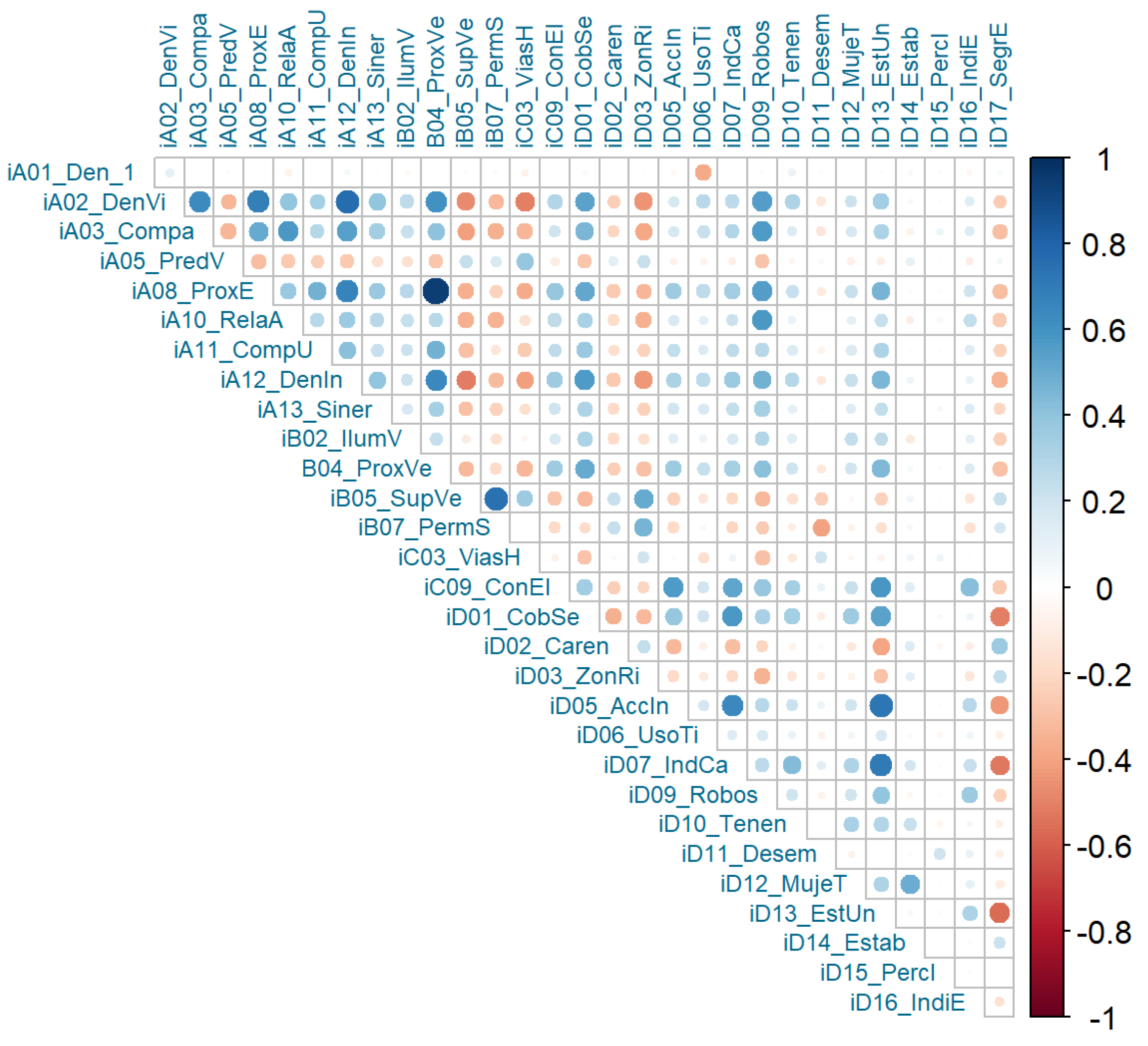
Figure 3.
Scree plot for the top 10 components in terms of variance explained.
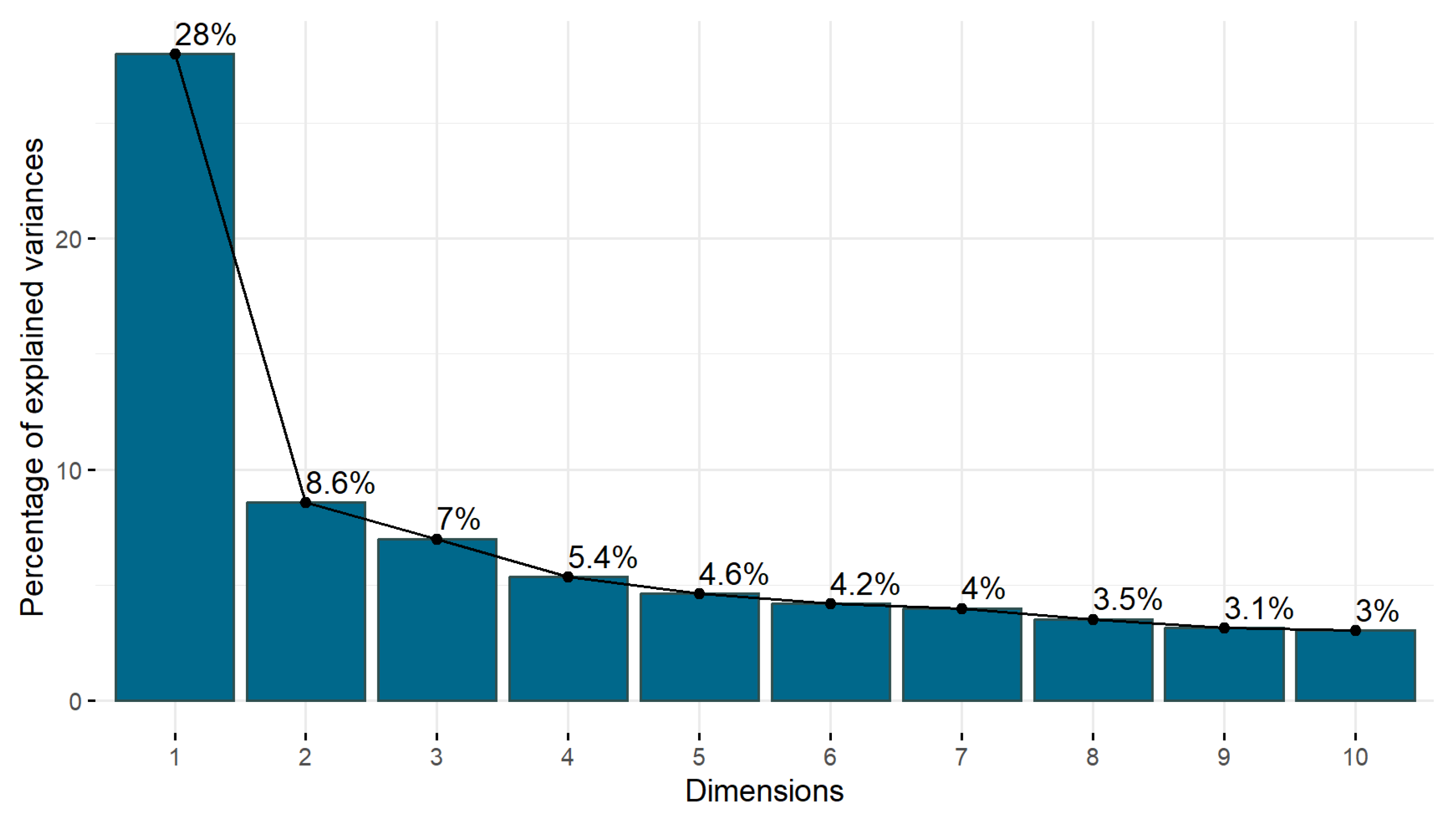
Figure 4.
Boxplots of the composite sustainability index by UFT, in ascending order.
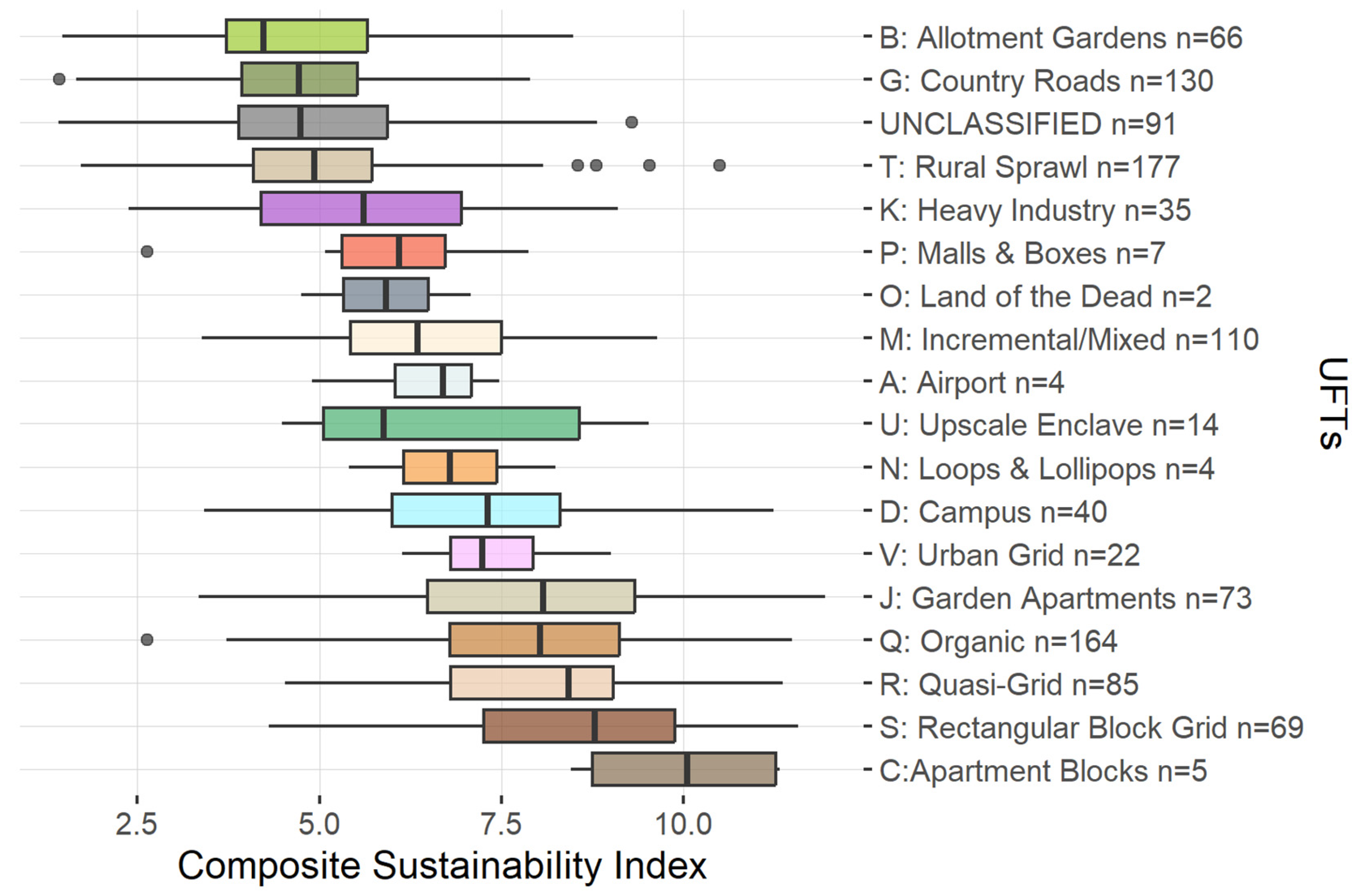
Figure 5.
Circular barplot of composite sustainability classified by high-level dimension and by UFT, in ascending order (clockwise).
Figure 5.
Circular barplot of composite sustainability classified by high-level dimension and by UFT, in ascending order (clockwise).
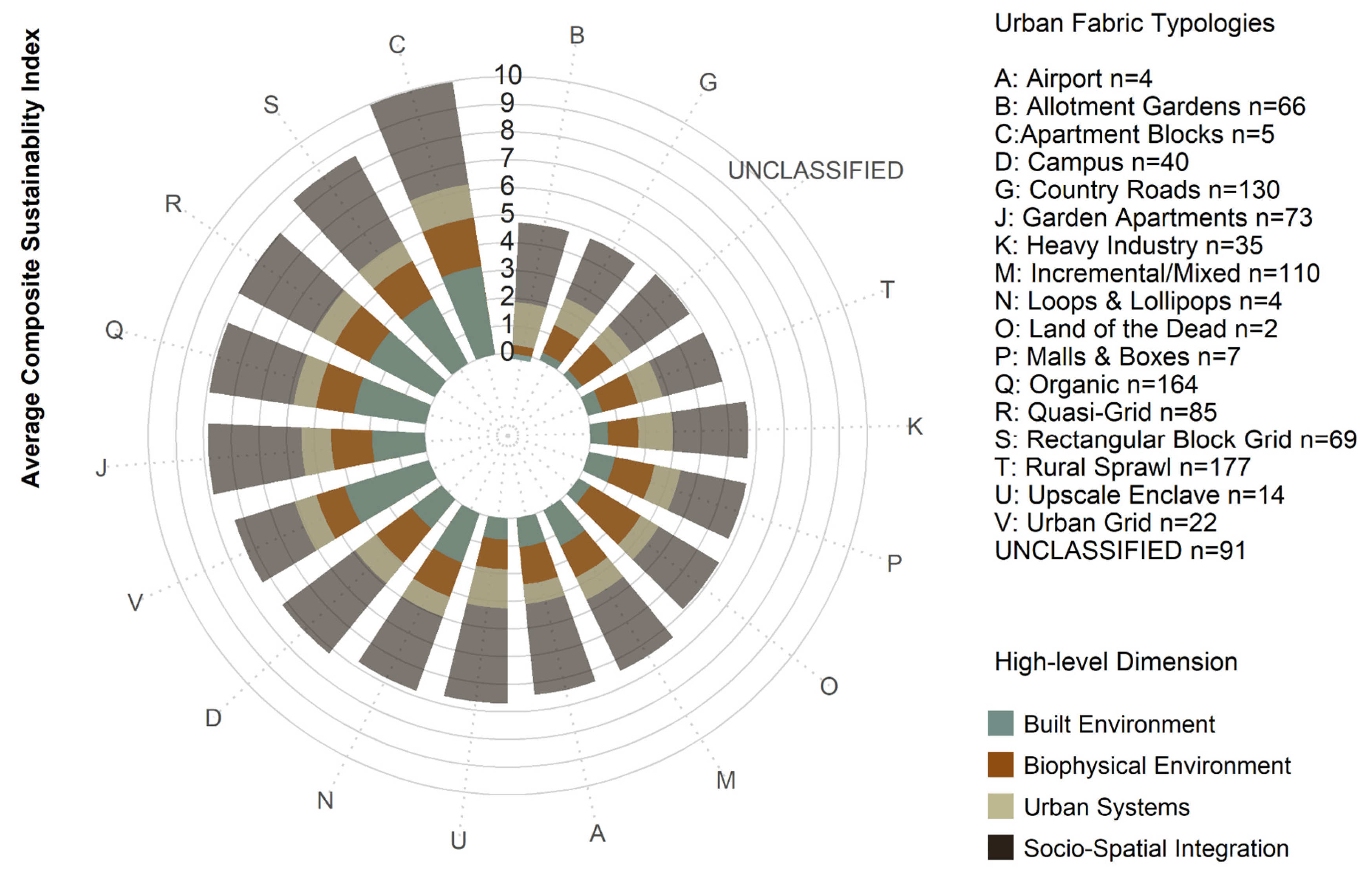
Figure 6.
Spider chart of UFTs with the 3 highest and 3 lowest composite sustainability, decomposing it by USIs.
Figure 6.
Spider chart of UFTs with the 3 highest and 3 lowest composite sustainability, decomposing it by USIs.
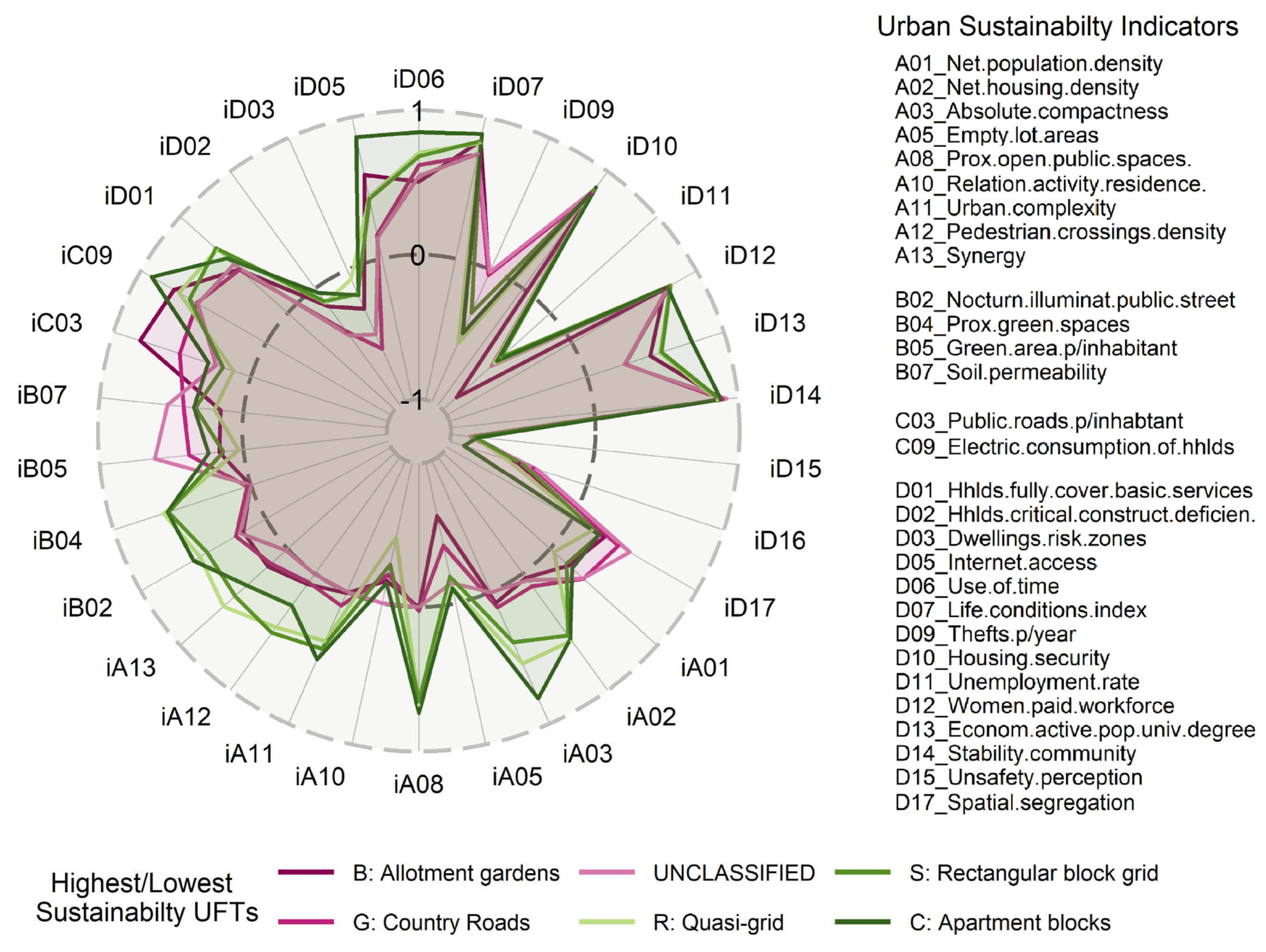
Figure 7.
Choropleth of Cuenca´s composite sustainability index, labelled by UFT.
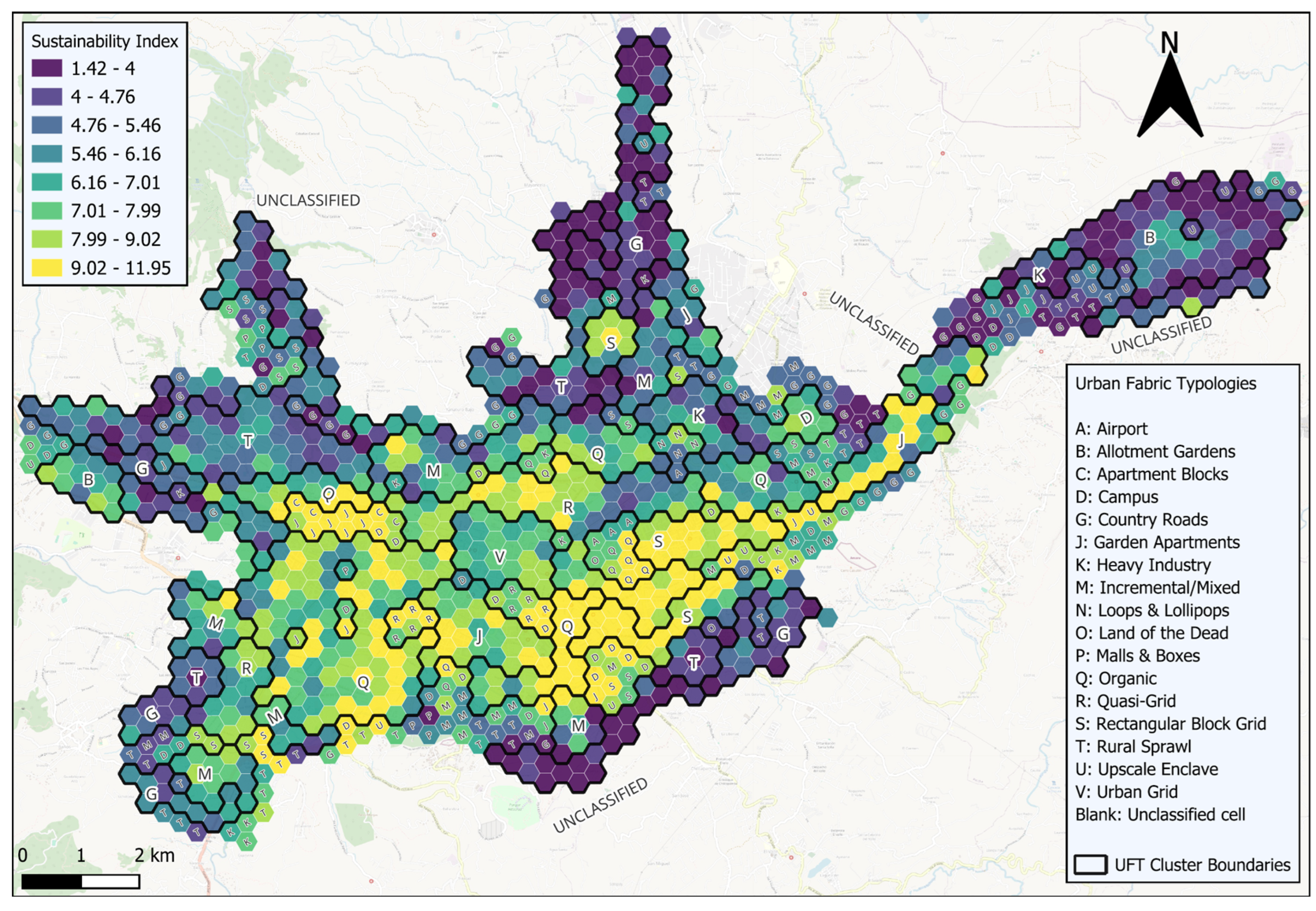
Figure 8.
Choropleth of Cuenca´s composite sustainability index, characterised by the two highest and two lowest sustainability index ranges and labelled by UFT.
Figure 8.
Choropleth of Cuenca´s composite sustainability index, characterised by the two highest and two lowest sustainability index ranges and labelled by UFT.
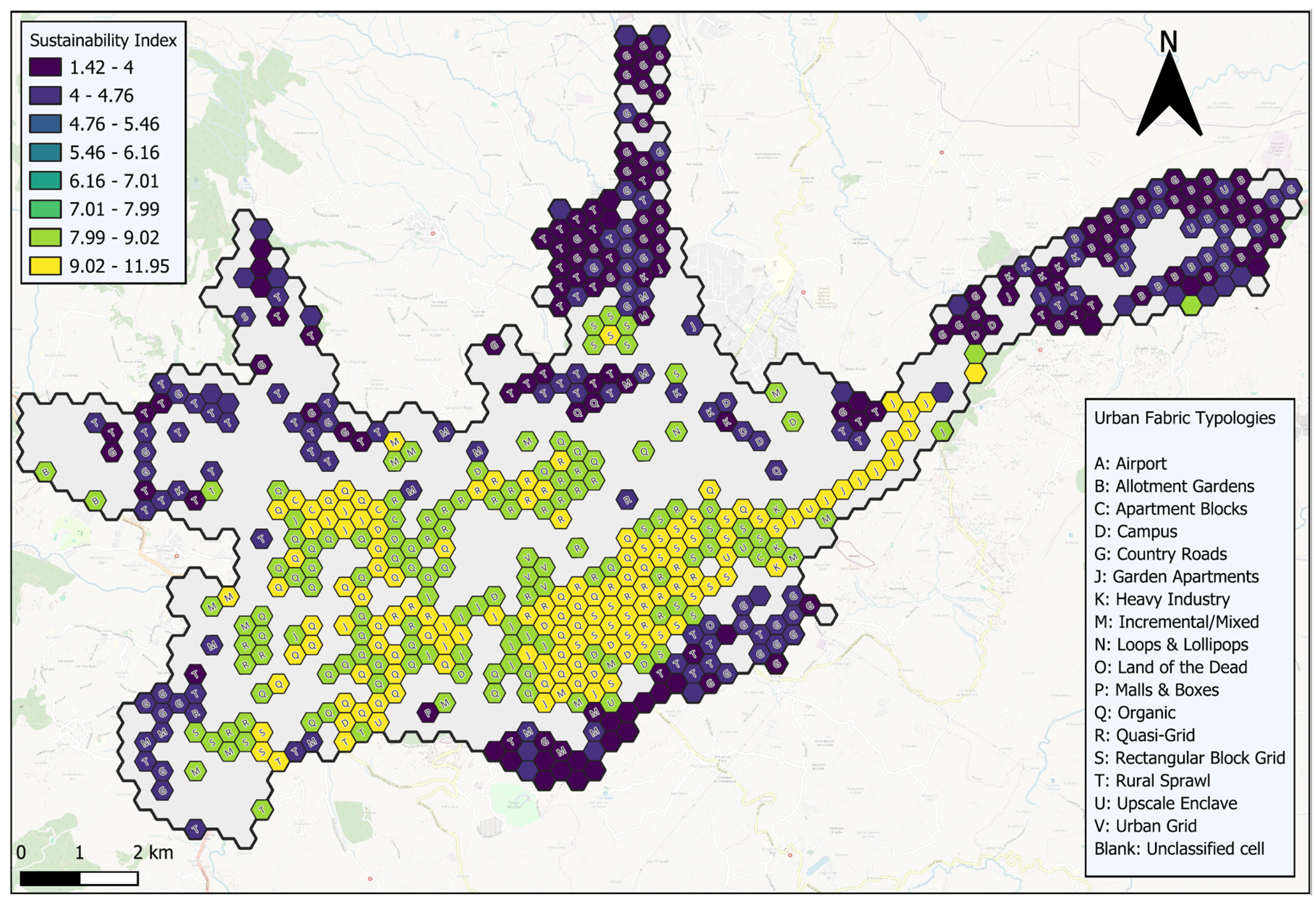
Figure 9.
Spatial patterns for each high-level sustainability dimension.
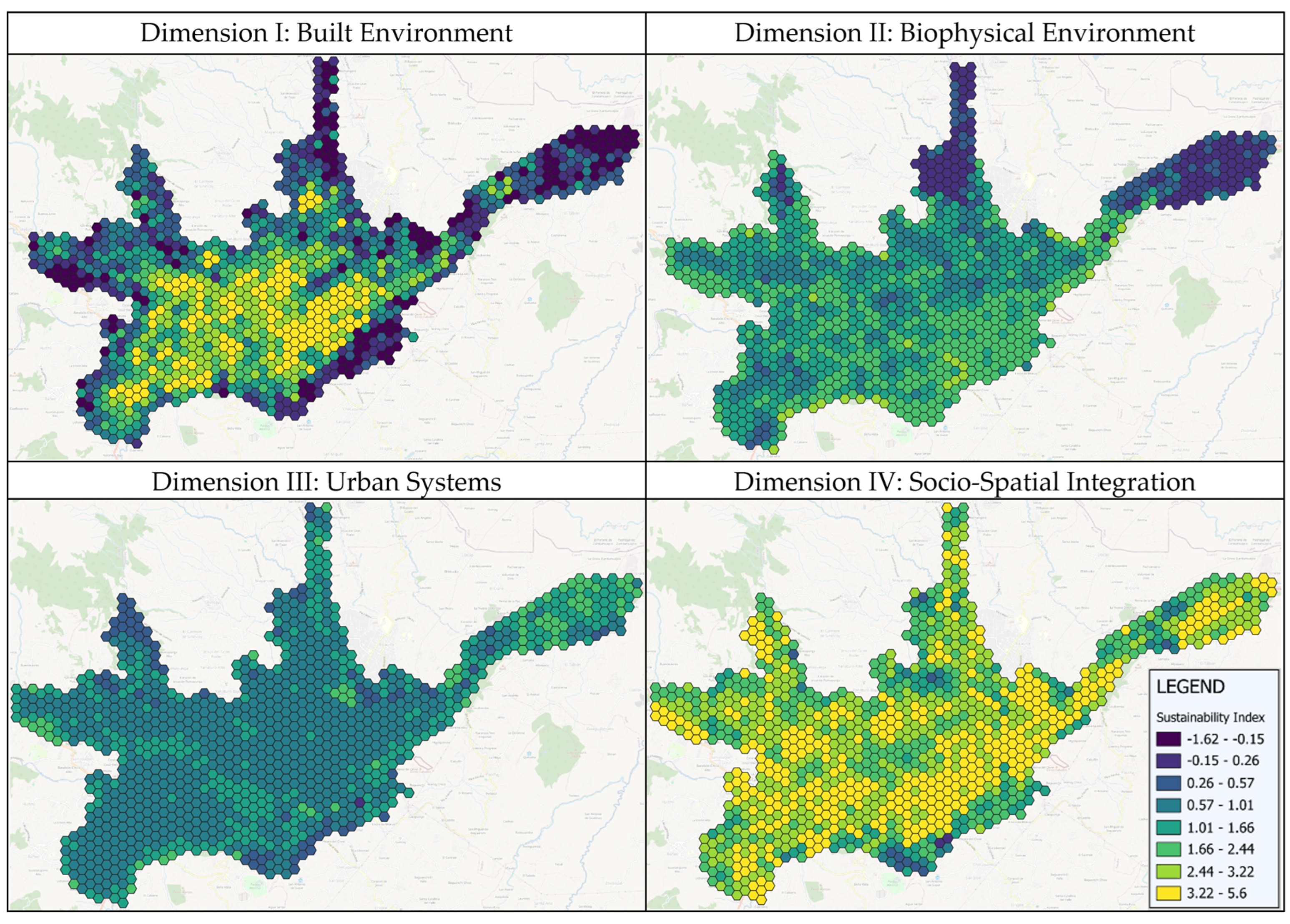

Table 1.
Characteristics of the study area.
| Study Area: Cuenca (as of 2022, the latest national census)1 | |
| Area | 7248.23 ha |
| Inhabitants | 361524 |
| Households | 115477 |
| Population Density | 49.87 inh/ha |
| Household Density | 15.93 households/ha |
Table 2.
Sustainability indicators for the city of Cuenca.
| No. | Name | Description |
| Dimension I: Built Environment | ||
| A01 | Net population density | Number of Inhabitants per hectare. |
| A02 | Net housing density | Number of houses per hectare. It evidences the consumption of residential land. |
| A03 | Absolute compactness | Building intensity equivalent to building volume on a given surface. |
| A05 | Empty lot areas | Percentage of unused land or buildings on the block. |
| A07 | Proximity to basic urban facilities | Percentage of households with simultaneous access within 500m to all types of basic urban facilities. |
| A08 | Proximity to open public space | The percentage of households within a 5-minute walk of at least one type of open public space (park, plaza, sports field, riverbank, open market). |
| A09 | Accessibility to purchasing basic daily supplies. | Percentage of households with simultaneous coverage within a 300m radius of different basic supplies necessary for daily life. |
| A10 | Relation between activity and residence | Urban variety and equilibrium are measured by the proportion of non-residential economic activities (commerce, services, offices) and the number of households. This indicator reflects a territory’s capacity to be self-contained in terms of mobility. |
| A11 | Urban complexity | Diversity and frequency of land uses. It relies on Shannon´s formula of entropy [32] to evidence the mixture of activities. |
| A12 | Pedestrian crossings density | Pedestrian connectivity of a territory, as the proportion of street pedestrian crossings to the whole study area. |
| A13 | Synergy | Degree to which the internal structure of an observational unit relates to a higher scale at the system level, according to spatial syntax theory. |
| Dimension II: Biophysical Environment | ||
| B01 | Air quality index | Amount of population not exposed to emission levels beyond the maximum permitted by Ecuadorian normative. Contaminants considered simultaneously (NO2, CO, SO2, O3, MP2.5, and MP10). |
| B02 | Nocturnal illumination of public streets | Proportion of the number of illumination devices to the lineal kilometres of public streets. Measures the perception of safety associated with illumination. |
| B03 | Acoustic comfort | Amount of population not exposed to noise levels beyond the maximum permitted by Ecuadorian normative. Max noise levels are 70dB at day and 65dB at night. |
| B04 | Proximity to green spaces | Closeness of the population to the nearest green space. |
| B05 | Green area per inhabitant | Ratio of public green space and the number of inhabitants. |
| B07 | Soil permeability | Area of permeable soil with respect to total area. It relates to loss of permeability caused by urban expansion, in terms of buildings and pavement. |
| Dimension III: Urban Systems | ||
| C03 | Public roads per inhabitant | Ratio of public road lanes (lineal metres) and population. |
| C04 | Proximity to alternative transport networks | Percentage of the population with simultaneous access to at least three alternative transport networks within 300m (bus, public bike share, bike paths, pedestrian paths; 500m for tram). |
| C09 | Electricity consumption of the household | Ratio of electricity consumption of the household by the number of residents in the household. |
| C13 | Wastewater coverage | Percentage of households connected to the public wastewater system. |
| Dimension IV: Socio-Spatial Integration | ||
| D01 | Households fully covered by basic services | Percentage of households with simultaneous access to drinkable water, electricity, wastewater and solid waste disposal. |
| D02 | Households with critical construction defects | Percentage of households with critical construction defects (that can endanger residents). |
| D03 | Dwellings located at risk zones | Percentage of households located at risk zones (landslide, flooding, topographically compromised, geologically compromised, agricultural zones, forestry zones, natural protection zones). |
| D05 | Internet access | Percentage of households that can connect to internet services by computer or mobile. |
| D06 | Use of time | Average time spent on personal activities within a working week (Mon-Fri), for the population aged 12 years and older. |
| D07 | Life conditions index | Level of scarcity or abundance of the following household variables: a) physical characteristics; b) basic services; c) education of residents aged 6 years and older ; d) access to health insurance. |
| D08 | Closeness and access to food | Spatial distribution of the city in terms of food purchasing locations (understood as: within 10 minutes from a public market). |
| D09 | Thefts per year | Ratio of thefts to people, households, institutions, retail and vehicles in the study area, to the total thefts in the city. |
| D10 | Housing security | Percentage of households with secured access to a dwelling (owned or rented). |
| D11 | Unemployment rate | Percentage of the economically active population (aged 15 and older) that is unemployed. |
| D12 | Women at paid workforce | Percentage of paid women in the workforce with respect to total employment (excluding agriculture). |
| D13 | Economically active population with a university degree | Percentage of the economically active population (aged 15 and older) with a completed university degree. |
| D14 | Stability of community | Percentage of the population living in the same place (parish) for 5 or more years. |
| D15 | Unsafety perception | Percentage of citizens that feel unsafe in their neighbourhoods. |
| D16 | Population ageing index | Quantitative ratio of older-adult population (aged 65 and more) to infant-young population (aged 0 to 15). |
| D17 | Spatial segregation | Level of exclusion, cohesion or segregation of the population with greater shortcomings (who fall within the first quartile of the Life Quality Index). |
Table 3.
Urban fabrics for the city of Cuenca.
| UFT | Code | Description |
| Airports | A | Large access roads, landing strips or parking spaces for transport buses. Land use is commercial, with large-scale terminal buildings and parking. Few green spaces. |
| Allotment gardens | B | Lane access is generally narrow and not paved. Housing units have ample green or recreational spaces; they may also have small agriculture fields. Parking is usually external to the garden area. |
| Apartment blocks | C | Medium and large blocks with moderate connectivity. Multifamily residences with shops or offices on the ground floor. Buildings are relatively tall (at least three stories). Parking lots and scarce green spaces. |
| Campus | D | Internal circulation routes. Single-use large plot (institutional, corporate or recreational). Buildings are scattered on the site, with parking lots and green areas. |
| Country roads | G | Develops linearly following rural paths. Connectivity is deficient, intersections are infrequent and there is no formal block pattern. Long and narrow plots. Single-family homes, small multi-family buildings and some shops. Agricultural fields and open spaces. |
| Garden apartments | J | Access roads to the apartment buildings; however, connectivity is deficient. Large plots of multifamily residences, with parking spaces, and many green and recreational areas. |
| Heavy industry | K | Access roads are irregular, and blocks are large. Land use is intended for heavy manufacturing. Large-scale buildings, warehouse spaces and parking. Vegetation is minimal. |
| Incremental/mixed | M | Generally rectilinear streets with disordered patterns and bad connectivity. Block’s size and shape vary. Single family homes, some multifamily buildings and shops. Density varies between low and moderate. There may be plantations and random green spaces. |
| Loops & lollipops | N | Curvilinear and irregular streets. Land use is mainly single-family residential, there may be multifamily buildings and shops. Plots are homogeneous, and dwellings are usually row houses. Parking is on the street or at the entrance. There may be neighbourhood parks. |
| Land of the dead | O | Usually fenced to restrict access from the outside. Single-use large plot (burial). Small services and parking buildings. Abundant green area and trees. |
| Malls & boxes | P | Usually connected to main streets, avenues or highways. Large plot of commercial use with typically low but large buildings. Parking lots and minimal vegetation. |
| Organic | Q | Street patterns are irregular and according to the topography with moderate connectivity. Land use is mixed, and density varies from moderate to high. Buildings are diverse in form and scale. Parking lots can be on the street, and there are occasional parks. |
| Quasi-grid | R | Street patterns are rectilinear but irregular, with high connectivity. Block’s size and shape vary, and plots are small to medium size. Building’s shape is diverse and present small retreats. Green spaces and occasional parking lots. |
| Rectangular block grid | S | Streets form a regular grid of rectangular blocks, with high connectivity. Homogeneous plots of residential and commercial use. Row houses, and some multifamily or duplex buildings may exist. Parking lots are in the street or at the entrances. Occasional small parks. |
| Rural sprawl | T | Few discernible blocks and low connectivity, it is located near urban access roads. Land use is mostly residential, there may be small shops, offices and multifamily residences. Buildings size vary and retreats are present. Lot of vegetation and original ecosystem remnants. |
| Upscale enclave | U | Usually a closed set, with varied street patterns and bad connectivity. Low density. Plots are generally large with exclusive single-family homes. Parking lots are located in adjacent garages or at the houses’ entrance. Gardens and communal recreational areas. |
| Urban grid | V | Well-connected rectilinear streets that form a grid pattern. Blocks are small and have a mixed land use. Buildings’ size and scale vary and may have interior patios. There are lots and parking buildings. Formal parks and plazas (civic squares). |
Table 4.
Results from individual one-way ANOVA tests.
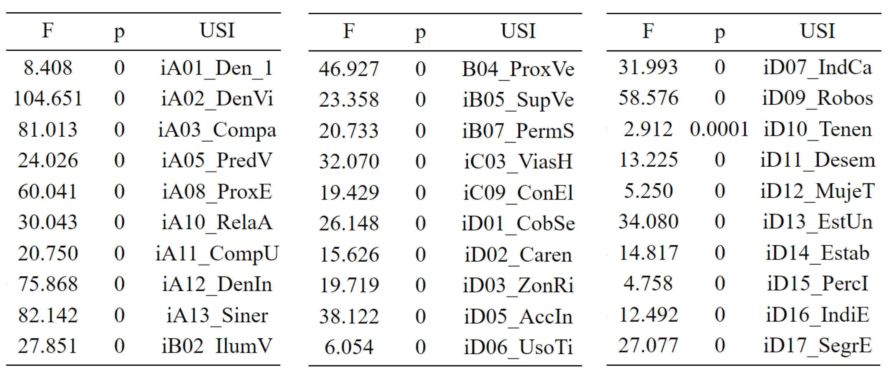
Table 5.
Results from Tukey’s Honest Significant Differences test.
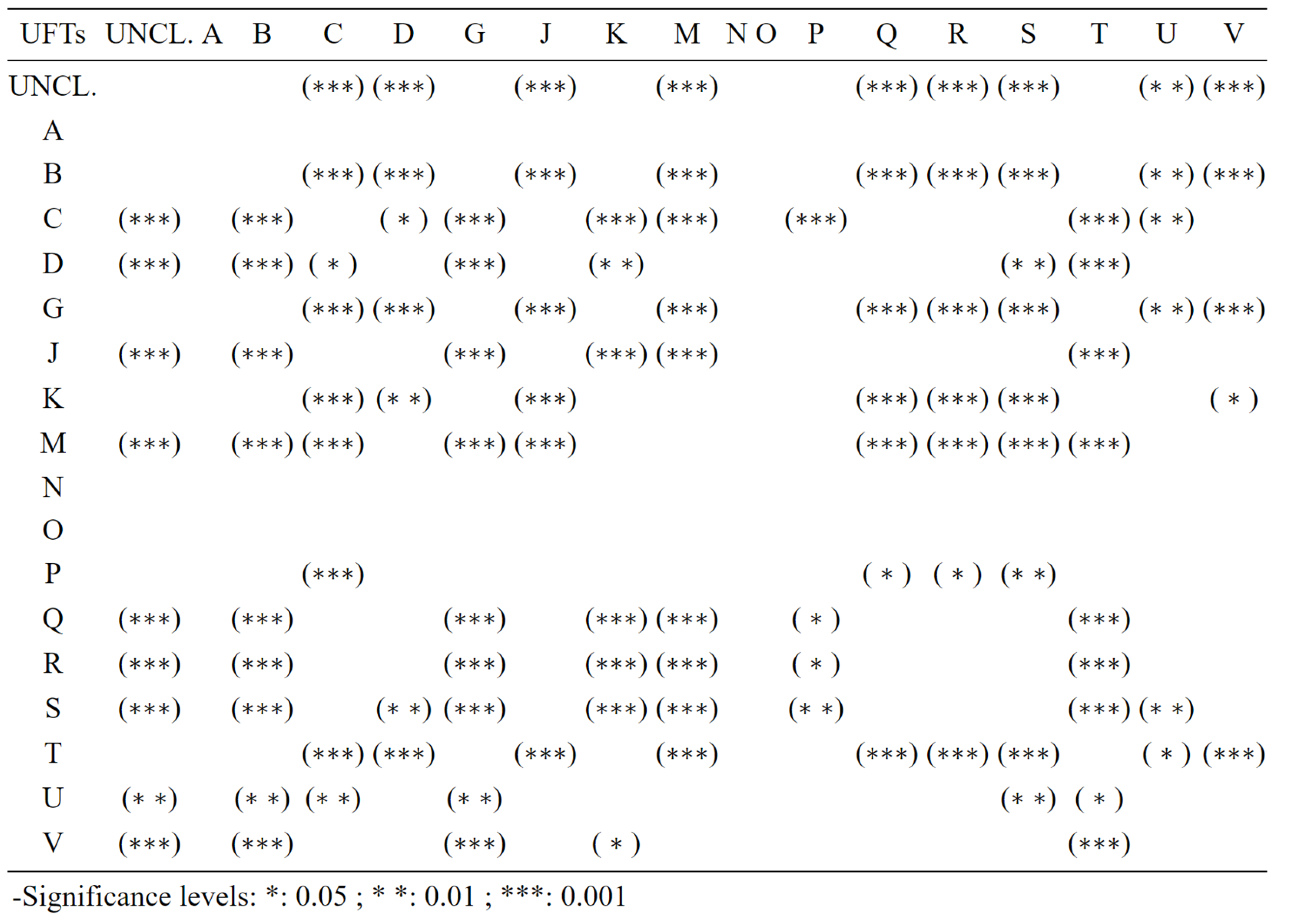
Disclaimer/Publisher’s Note: The statements, opinions and data contained in all publications are solely those of the individual author(s) and contributor(s) and not of MDPI and/or the editor(s). MDPI and/or the editor(s) disclaim responsibility for any injury to people or property resulting from any ideas, methods, instructions or products referred to in the content. |
© 2024 by the authors. Licensee MDPI, Basel, Switzerland. This article is an open access article distributed under the terms and conditions of the Creative Commons Attribution (CC BY) license (http://creativecommons.org/licenses/by/4.0/).
Copyright: This open access article is published under a Creative Commons CC BY 4.0 license, which permit the free download, distribution, and reuse, provided that the author and preprint are cited in any reuse.


