
Submitted:
27 July 2024
Posted:
30 July 2024
You are already at the latest version
Abstract
This paper investigates the long-run relationship between the U.S. dollar and Canadian dollar by defragmenting the bilateral exchange rate induced by nominal and real shocks. The methodology centers on a structural vector autoregressive (SVAR) model, including the analysis of impulse response and variance decomposition to account for the impact of nominal and real shocks on exchange rate movements. The study also decomposes the real shocks into demand and supply factors from both Canada and U.S. and compare their impact on the nominal and real exchange rate. Results are compared to shocks driven by country specific nominal factors. The study is conducted using quarterly based data over December 1972 – December 2023. Findings suggest that the real shocks have a permanent impact on both the nominal and real exchange, compared with nominal shocks which have a temporary impact. Country-specific real supply-side factors have a more discerning impact than country-specific real demand-side factors. Country-specific nominal barely impacted the nominal and real exchange between U.S. and Canada.
Keywords:
long-run relationship
; structural VAR
; U.S. dollar
; Canadian dollar
; shocks
1. Background to Study
Five keywords are making the buzz in the headlines nowadays. Dubbed as the 5D’s, they are namely deglobalization, decarbonization, demographics, debt, and dovish policies [1]. These secular factors are directly contributing to inflation, at a structural level, in major developed economies, including Canada and U.S. Since COVID-19, deglobalization and decarbonization have added to volatility of prices globally. For instance, while the consumer price index (CPI) changed from 1.2% in 2020 to 8% in 2022, before dropping by 4.1% on a year-to-year percentage change; Canada also experienced a similar trend with CPI changing from 1.4% in 2020 to 6.8% in 2022, before falling by 3.9% in 2023. During the same period, the trade balance relative to the Gross Domestic Product (GDP), ranged between -3.9% (2023) and -4.6% (2022) in the U.S. Comparatively, Canada has, after 10 years of witnessing negative values, started to continuously report positive trade balances, ranging between 0.4% and 1.2% of the nation’s GDP. Post COVID-19, both developed economies reported real GDP which were increasing, on a year-to-year basis, at a decreasing rate, with U.S. (Canada) real GDP increasing at 2.5% (1.1%) respectively [2]. Further, while the wholesale price indices (WPI) for both countries are positive correlated, the nominal exchange rate between the Canadian dollar fluctuated between 0.7 U.S. dollar (USD) per Canadian dollar (CAD) to 0.8 U.S. during the period 2020-early 2024. Finally, imports have been dropping for both developed entities, with U.S. (Canada) experiencing a fall of 4.9% (2.2%) in 2023. In the same vein, exports dropped in U.S. (Canada) by 2.2% (5%) respectively. Energy commodities such as crude oil have not been spared either, with the West Texas Intermediate WTI) crude oil futures price fluctuating between $20 per barrel in 2020, reaching a settlement price of $103.89 in March 2022, and trading around $80 per barrel in early 2024 [3].
One of the major causes of price volatilities in commodities can be attributed to government actions regarding climate change and the investors gradually orienting their investments towards sustainable equity finance [4]. While government-based initiatives on pushing for faster decarbonization and reduced greenhouse emissions are plentiful, with sometimes globalized cooperation among various key global players such as U.S. and Canada [5], the mechanism towards a green transition has also led to a more localized focus. For instance, the rise of carbon pricing implementations and increased interest in local renewable energies led to various countries adopting protectionist measures, as a fuel to deglobalization. While globalization brought a delocalization of production to geographical areas with lower costs of production and lower environmental standards, policy makers in the U.S. are promoting the adoption of strategies met to bring production back to the leading nation. As an example, the Inflation Reduction Act necessitates part of a product to be U.S. made. [6] posits that while on-shoring or near-shoring the production of strategic goods such as minerals can allow countries to benefit from lower transportation costs and avoid supply-chain issues, multilateralism is recommended by sanctioning countries who pursue aggressive trade policies or wars against other countries.
Alternatively stated, post COVID-19 supply chain disruptions, the Russian-Ukraine war, and US-China trade war can be attributed as major causes of fluctuations in current trade activities and commodity prices globally. Price increases in energy commodities, particularly in crude oil and natural gas, affect each nation differently, based on whether the economy is an importer or exporter of commodities in general [7]. For instance, it was found that exchange rate fluctuations for commodity currencies such as the Australian dollar was mostly due to gas price shocks caused by the ongoing war in Ukraine [8].
Canada is of particular interest, as it is a major consumer, producer, and exporter of energy. Specifically, Canada is among the top ten producer of natural gas, oil, hydropower, uranium, nuclear power, biofuels, and wind. Energy contributes to 10% of the country’s GDP, with the petroleum and electricity industry contributing 7.2% and 1.7% [9]. The energy sector also represents a major stream of capital investments and trade flows [10]. Even though the country has a broad range of free trade agreements with about 70% of the global economy, demand for exports has been mostly driven by the U.S. While it can be argued that the termination of the North American Free Trade Agreement (NAFTA) had a negative impact on Canadian exports, the effect was offset by the Canada-United States-Mexico Agreement (CUSMA) in mid-2020 [11]. With major industries based in the primary sector, Canada is the fourth (fifth) largest producer of crude oil (natural gas) globally, with also the third largest oil reserves. More than 95% of its oil is exported to the U.S. [12]. Conversely, 60% of U.S. imports come from Canada [9]. In addition to its huge reserves of natural gas, Canada is the fourth largest metallurgical coal exporter, after Australia, Russia, and the U.S. [13]. 100% of Canada’s exported electricity is destined for U.S., with 92% of U.S. imported electricity coming from Canada. Finally, Canada is the second largest exporter of uranium globally [14], with 64% of its exports heading to the U.S, Europe [15].
In light of the above background on the critical importance of the energy sector in Canada, the trade dynamics between Canada and U.S., and several additional factors which are currently affecting the global financial markets including deglobalization; localized decarbonization with Canada’s sustained commitment to the phase-out conventional coal-fired electricity nationally by 2030 [10]; the Russia-Ukraine war; and U.S-China trade war, it is imperative to investigate the relationship between the Canadian dollar and U.S dollar. Specifically, it is added-value to understand which country-specific factors drives the exchange rate between the two countries, especially given that they are important trading partners to each other; both countries are leading consumers, producers, and exporters of energy globally; and the Canadian dollar per U.S. dollar is one of the most actively traded currency pairs.
While it is expected that a structural model constructed to determine exchange rates should be able to shed light on variables which contribute to nominal and exchange rates changes, evidence from the extant literature is mixed. For instance, while [16,17] find no cointegrating relationships between bilateral exchange rates and various macroeconomic indicators. Comparatively, more recently, [18,19] found more significant relationships between macroeconomic factors such as oil price, and interest rates differentials and exchange rates. Importantly, [20,21] support that macroeconomic models can be limited in terms of the information included in exchange rate determination.
Instead of regressing macroeconomic variables onto exchange rates, we borrow and extend [22] by adopting the technique proposed by [23] to defragment exchange rates movement into the changes induced by nominal and real factors. Alternatively stated, for the purpose of our study, we decompose the Canadian dollar relative to the U.S. dollar into movements caused by nominal shocks compared to those caused by real shocks. Our primary contribution is to further understand the long-run relationship between the Canadian dollar and U.S. dollar in an unprecedented period backed by deglobalization and decarbonization. Specifically, we showcase the differential impacts of real and nominal shocks using impulse responses and variance decompositions on nominal and exchange rates. In line with prior literature, we further decompose the real shocks into demand and supply driven factors and analyze the impact of these country-specific factors onto the nominal and real exchange rate. This also enables us to compare country-specific real demand and supply shocks to country-specific nominal shocks on the exchange rate. We differ from [22] in two important aspects. Firstly, we are extending the data analysis from 1973-1992 to December 1972- December 2023, thereby giving us a more important gauge of the long-run relationship between the two countries’ currencies. Secondly, we are analyzing the effect of real government expenditure, real GNP, and nominal money supply onto the nominal and real exchange rate, compared to the earlier study which analyze the impact of the ratio of log real government expenditure in one country relative to the other country, the ratio of log real GNP between both countries, and the ratio of log nominal money supply between the two countries. Since we are more interested in the impact of country-specific shocks onto the real and nominal exchange rate, we retained the use of the log of demand/supply variables and money supply factors from Canada and U.S.
The rest of the paper is organized as follows: Section 2 provides some literature reviews on exchange rate determination, commodity currencies, real and nominal exchange rates, and the demand and supply factors affecting exchange rates. Section 3 summarizes the methodologies and data used. Section 4 provides the data and some preliminary analysis. Section 5 provides the research findings. We rest our case with some conclusive remarks.
2. Literature Review
2.1. Exchange Rate Determination
The US and Canadian dollars are major world currencies and as such have drawn a significant amount of attention in academia. There exist swathes of research that examine the relationship between the two currencies using different methodologies. The effects of oil shocks on the US exchange rate have been well-documented [24,25]. A new adjusted relative strength index was employed to study the connection between energy markets and exchange rates in [26]. The findings suggest an inverse relationship between energy and currency markets. Other commodities such as gold have also impacted the currency exchange rates [27].
Trade is a major factor in determining exchange rate. [28] have shown the role of the balance of trade in determining the exchange rates. Covered interest parity and contractions of cross-border bank lending in dollars were shown to go hand in hand with strong US dollar [29]. The authors reveal the role of the dollar as a key barometer of risk-taking capacity in global capital markets. [30] show that quantity elasticities are significantly below one and export prices are significantly affected by exchange rate changes. [31] shows the interaction between the US dollar and international trade. The study reveals a novel channel of exchange rate transmission that goes in the opposite direction to the competitiveness channel.
Monetary and fiscal policy have been studied as major drivers of exchange rate. The effects of monetary policy regime on the relative importance of nominal exchange rates were studied by [32] who find that the current real exchange rate predicts future changes in the nominal exchange rate. The effects of monetary policy announcements on exchange rate dynamics in the US has been studied by [33]. The results suggest that while the short-run effects on the exchange rate are mainly due to policy shocks, the medium-run response is guided by information effects. Similarly, the effect of monetary policy surprises on the exchange rate behavior was studied by [34] who found that conditioning on possible information effects driving longer term interest rates, there appear to be additional drivers of exchange rates. Fiscal shocks such government spending has been shown to affect the real exchange rate. The study by [35] implies that the impact of public sector expenditure changes across different types of spending, with shocks to public investment generating larger and more persistent real appreciation than shocks to government consumption.
Global shocks have also been shown to affect the exchange rates. The effects of extreme events such as Covid-19 and the war in Ukraine have been studied [36,37,38] develops a model in which specialized bond investors must absorb shocks to the supply and demand for long-term bonds in two currencies. The proposed model matches several important empirical patterns, including the co-movement between exchange rates and term premia. The study also finds that central banks’ quantitative easing policies affect exchange rates.
2.2. Real and Nominal Shocks
[39] study documented the sensitivity of exchange rate and trade balance to the real shocks such as supply and demand disruptions. In case of highly interconnected economies like Canada and the USA the demand shocks may lead to a substantial fluctuation in the bilateral exchange rate due to changes in import and export levels. This also applies to the supply shocks like the change in natural resources availability, geopolitical stability, natural disasters, or technological advancement that directly affect the production capacity and trade flow between countries, such issues can significantly and immediately affect the bilateral exchange rate [40]. For instance, the fluctuation in oil price may cause immediate and significant demand shock. In details, the increase in oil prices will lead to an appreciation of the CAD relative to the USD since the Canadian economy relies on oil export [41]. On the supply side, unexpected and sudden changes in the production level due to technological advancement or disruptions in supply chains (e.g. COVID 19) or natural disaster can cause a supply shock. These shocks have a variant impact on the currencies exchange rates through the change in the prices of goods and services between the two countries.
On the other hand, the monetary approach to exchange rate theory is the main source of information about the link between money supply and exchange rates. According to this theory, a currency's supply and demand, which are impacted by variables like interest rates, inflation forecasts, and economic growth, determine its price [42]. This theory states that, all else being equal, a rise in a nation's money supply raises inflation and decreases demand for that nation's currency, which causes it to weaken. Thus, when the money supply is reduced, foreign capital tends to be attracted to higher interest rates and lower inflation rates, which leads to currency appreciation [43,44]. This perspective also empirically approved, studies utilizing structural Vector Auto-Regression (VAR) models and cointegration analysis indicate that demand and supplies shocks can raise significant and long-term changes in the behavior and dynamics of currency exchange rates [45].
The exchange rates fluctuation also might be affected due to nominal shocks, typically arise from the change in money supply and countries monetary policy. For instance, the inflation expectations and interest rate are directly and positively associated with the money supply, causing increase of inflation and depreciating the currency value. This depreciation can initially have a negative impact on countries’ trade balance, as imports become more expensive, and exports increase without experience a corresponding growth in foreign demand. However, the long-term effects of these nominal shocks can vary depending on the elasticities of demand for traded goods and the speed at which prices adjust in both local and foreign markets. These effects are vital to explore and understand the nominal dynamics between the CAD and USD. In the context of CAD and USD, [46] delves deeply into this dynamic, explaining how policy differences between the Federal Reserve and the Bank of Canada can cause notable fluctuations in exchange rates. Research has indicated that significant swings in the CAD/USD exchange rate might result from divergences in the monetary policy outlook between the Federal Reserve and the Bank of Canada. For instance, the U.S. dollar is likely to depreciate in relation to the Canadian dollar if the Canadian monetary policy is contractionary and the U.S. monetary policy is expansionary [47].
Other literature discussed the impact of real government expenditure and currency demand shocks and documented that these two factors are pivotal in determining the exchange rate dynamics between the CAD and USD [48]. In this regard, real domestic currency depreciation is typically the result of expansionary fiscal policy, which is shown in more government expenditure. This is because such spending usually results in more aggregate demand than supply, which drives up local prices in comparison to overseas prices and lowers the actual exchange rate. Particularly, the government spending, monetary policy, and the real exchange rate align with the above discussion, as the government purchases increase leads to decline in the currency exchange rate due to the change in the country balance of payments and the goods and market equilibrium conditions [49].
2.3. Structural Vector Autoregressions
Recently, machine learning has been actively applied to model financial asset movements [50,51]. Particularly, it has been widely used to model exchange rate time series. [52] compared the performance of ten machine learning algorithms to forecast instances of significant fluctuations in currency exchange rates. The study finds that the proposed outlier detection methods substantially outperform traditional machine learning and finance techniques. Similarly, [53] compared several machine learning models to explore the predictability of exchange rate trends and found that a combination of long short-term model and convolutional neural network outperformed the Transformer model.
Structural vector autoregressions (SVARs) are a key type of time series model widely utilized for macroeconomic analysis. It is a well-established approach with solid theoretical underpinnings and wide range of applications [54,55]. This model includes multiple linear autoregressive equations that capture the combined movements of economic variables. The residuals from these equations are blends of fundamental structural economic shocks, which are presumed to be orthogonal [56]. With a limited number of assumptions, it is possible to estimate these relationships—known as shock identification—and describe the variables through linear equations of both current and past structural shocks [57]. The coefficients in these equations, termed impulse response functions, depict how the variables in the model react dynamically to shocks. Various methods for identifying structural shocks have been discussed in the academic community, including short-run restrictions, long-run restrictions, and sign restrictions [58,59,60]
SVAR models are frequently used to explore how macroeconomic shocks affect economies and to evaluate economic theories. [57] uses SVAR with a less restrictive formulation to analyze the impact of shocks to oil supply and demand. The author find that supply disruptions are a bigger factor in historical oil price movements and inventory accumulation a smaller factor than implied by earlier estimates. SVAR models have been particularly focused on examining the impacts of monetary and fiscal policy shocks, along with other nonpolicy shocks such as those related to technology and finance. [61] employed SVAR to study the response of asset prices to monetary policy shock in Indonesia. These results suggest that an increase in monetary policy interest rate appreciates exchange rate, lowers the stock price, and reduces bond yield. The SVAR model was used to investigate structural shocks in monetary policy, exchange rates, and stock prices in Iran. The results suggest that structural shock on the exchange rate does not affect the stock price, but the monetary policy's structural shock positively impacts the real exchange rate. Recently, the effects of Covid-19 on the price of SP500 were investigated by using a SVAR model. The results imply that a 1% increase in cumulative daily COVID-19 cases in the US leads to an approximately 0.01% cumulative reduction in the S&P 500 Index after 1 day [62].
3. Methodology
3.1. Nominal and Real Exchange Rate
While a nominal exchange rate reflects the price of one currency against another, the real exchange rate (RER) attempts to measure the value of a country’s goods against those of another country, a group of countries, or the rest of the world at the prevailing nominal exchange rate [63,64,65]. RER is expressed as follows:
where is the real exchange rate between 2 countries (x and y); is the nominal exchange rate, and is the wholesale price ratio between the 2 countries. For example, the real exchange rate between US and Canada would be The wholesale price index (WPI), as opposed to the consumer price index (CPI), focuses on the price of goods traded by corporations [66].
3.2. Structural VAR Model
Assume and are the zero-mean mutually uncorrelated real and nominal shocks, respectively. Formally, a 2 x 1 vector of the first differences in real and nominal exchange rates, , can be illustrated with a bivariate moving average representation as follows:
where is the real exchange rate at time period t ; is the nominal exchange rate at time t; = is the real shock at time t ; is the nominal shock at time t ; (L) for i, j=1, 2 is an infinite-order polynomial in the lag operator L ; is the first-difference operator ;and the innovations are normalized such that Var(= I. The time paths of the effects of the various shocks on the real and nominal exchange rates are implied by the coefficients of the polynomials (L). The restriction that the nominal shocks have no long-run effect on the real exchange rate is represented by the restriction that the sum of the coefficients in sum to zero; thus if (k) is the kth coefficient in (L):
Since (j) is the effect of on after j periods, is the cumulative effect of on over time. Similarly, because = is the effect of on in the long run . Subsequently, the restriction that implies that the cumulative effect of on over time is zero, and that is the long run effect of on r is zero. Alternatively stated, the nominal shock has only short-run effects on real exchange rate, whereas the real shock may have long run effects.
4. Data
In addition to the important role Canada plays on the global arena and with its U.S. counterpart, it is important to understand the two countries’ relative importance in trades. Consistent with [67], the Canadian dollar and U.S. dollar are among the most actively traded currency pairs as per the Bank of International Settlements triennial 2022 survey [68]. Specifically, Figure 1 reports that, during the 2001-2022 period, the Canadian dollar represented between 4%-5% of all foreign currency trades, with a noticeable increase to 6.2% in 2022. Comparatively, the U.S. dollar remains the dominant currency globally, being present in between 85% and 90% of all trades.
Figure 2 displays the RER for Canada relative to the U.S. Due to the wholesale price index in Canada being always higher than in the US, this resulted in a lower RER. While this relationship has been maintained during the whole period under study, the spread between the NER and RER displays less (more) volatility in the short-run (long-run). From Figure 2, we interpret there are two kinds of shocks which we dub as nominal and real shocks. While the real shock affect both NER and RER in a similar way, the nominal shock affects the two rates distinctively. Consistent with the concept of long run neutrality [69], we assume the nominal shocks to have a temporary effect on RER. Alternatively stated, permanent changes in nominal variables have no effect on real variables in the long run.
This serves as the identification restriction to defragment the exchange rates time series. To remove the effect of outliers in the data, we use the log of US Real GNP to CAD real GNP as a supply shock measure (y), the log of US real government expenditure to CAD real government expenditures to capture demand shock, and the log of US nominal money supply (M1) relative to CAD nominal money supply as a proxy for nominal shock. All data were sourced from Factset.
4.1. Preliminary Analysis
Descriptive statistics including mean, median, standard deviation, skewness, kurtosis, the Jarque-Bera test for normality, the Augmented Dickey-Fuller (ADF) test, and the number of counts in each sample series are reported into Table 1 for the period of 29th December 1972 to 29th December 2023. We use M2 as a measure of money supply in line with [70] who finds the indicator, compared to other money supply indicators, to have a significant impact on economic growth in the short run. GNP, as opposed to Gross Domestic Product (GDP), as the size of the commodities sector and export orientation are two critical factors which could render GNP to be significantly different from GDP [71]. The average of WPI for Canada was higher than its US counterpart, resulting in wholesale price ratios which pushed the real exchange rate (RER) between the US and Canadian dollar to be lower than the nominal exchange rate (NER).
Although the average real government expenditure from US is almost 9 times that of Canada, normalizing each country's average with its own standard deviation, results in an average/standard deviation value of 4.11 and 3.97 for US and Canada respectively. Apart from the money supply for both countries, all variables exhibited negative kurtosis, with US real government expenditure and US real expenditure have the lowest kurtosis values. WPI for Canada (US) was negatively (positively) skewed. The nominal (real) exchange rate for USDCAD was positively (negatively) skewed. Except for US real government expenditure, all other government expenditure, real GNP, and money supply were positively skewed, with the latter exhibiting highest skewness. The p-value under the Jarque-Bera test reject the hypothesis of normality for all series, except for WPI for both countries and the nominal exchange rate for USDCAD. Except for the RER and wholesale price indices ratios, the p-values under the Augmented-Dickey-Fuller (ADF) test at 10% significance level, support that all the series are non-stationary at 5% significance level. This is in line with [72], where long-run restrictions in a structural vector requires at least one non-stationary variable. All variables were stationary after one-time differencing.
Table 2 reports the Pearson pairwise correlation coefficients and corresponding p-values. Both countries' wholesale price indices were strongly positively correlated with each other (0.988), and other macroeconomic indicators including real government expenditures, real GNP, and money supply, with correlation values ranging between 0.905 and 0.968. This supports the globalized impact of these two partner countries where their inflation policies (represented by WPIs), economic activity (real GNP) and monetary policy (money supply) measures are strongly positively linked with each other. While both WPI shared moderate positively correlations with the nominal and real USDCAD, both countries' inflationary measures were negatively correlated with the wholesale price ratio. More importantly, the nominal USDCAD was strongly negatively correlated with the wholesale price ratio (-0.795), with the real USDCAD also witnessing a negative correlation of -0.421 with the wholesale price ratio. Both real government expenditures were positively correlated with the nominal and real exchange rate. The wholesale price ratio was however negatively correlated with both US and Canada's real government expenditure, real GNPs, and money supply. However, the relationship between the wholesale price ratio and Canada's real GNP, and both countries' money supply were insignificant. Except for the abovementioned negative correlation between nominal USDCAD and the wholesale price ratio, NER had a weak but positive relationship with all other variables. Similarly, this was observed for the RER, which has a weak but positive relationship with real government expenditure, real GNP, and money supply. This can be explained by the strong positive relationship between the nominal and real exchange rate for the USDCAD. While both countries share the strongest positive correlation of 0.998 in their money supply values, money supply from each country had a smaller effect on the wholesale price indices for each country, compared to real government expenditure and real GNP. In light of the above preliminary analysis, we decompose NER and RER movements into the components produced by nominal and real shocks. While nominal shocks can only affect the USDCAD in the short run, real shocks can cause permanent effects on the USDCAD in the long run.
Prior to running the structural VAR model, we transform our data into log and check for stationarity using correlograms and the Augmented-Dickey-Fuller test, in line with [22]. From the correlograms of the nominal and real USDCAD illustrated in Figure 3, the autocorrelation function decays slowly supporting both level series are non-stationary. This is in line with [70], where long-run restrictions in a structural vector requires at least one non-stationary variable. Although not reported here, both NER and RER were stationary after one-time differencing.

Table 3.
Autocorrelations for December 1972- December 2023.
| ρ(k) | k = 1 | 2 | 3 | 4 | 5 |
| Without first order differencing | |||||
| NER | 0.961 | 0.916 | 0.879 | 0.838 | 0.796 |
| RER | 0.93 | 0.856 | 0.801 | 0.737 | 0.663 |
| With first order differencing | |||||
| NER | 0.081 | -0.101 | 0.036 | 0.016 | -0.057 |
| RER | 0.025 | -0.137 | 0.06 | 0.075 | -0.056 |
Note: ρ(k) represents the autocorrelation between and . NER (RER) denotes the nominal (real) exchange rate for USDCAD, where the latter represents the exchange rate for Canadian dollar per US dollar. Variables are in logs.
5. Research Findings
5.1. Lag Optimization
We first estimate a standard VAR model using both nominal and real exchange rates. Appropriate lag length is selected based on the lag length criteria recommended by Schwarz (SC), Hannan-Quinn (HQ) and Akaike information criteria (AIC). A lag of 1 is selected based on AIC and HQ information criterion. Although not reported here, correlograms show that the autocorrelations between differenced variables lies within 2 standard error bounds.
Table 4.
Standard VAR lag selection.
| Lag | LogL | LR | FPE | AIC | SC | HQ |
| 0 | 999.609 | NA | 1.300E-07 | -10.180 | -10.146 | -10.166 |
| 1 | 1010.102 | 20.663 | 1.220E-07 | -10.246 | -10.145 | -10.205 |
| 2 | 1012.760 | 5.181 | 1.230E-07 | -10.232 | -10.064 | -10.164 |
| 3 | 1015.074 | 4.462 | 1.260E-07 | -10.215 | -9.981 | -10.120 |
| 4 | 1019.371 | 8.201 | 1.250E-07 | -10.218 | -9.917 | -10.096 |
| 5 | 1021.178 | 3.411 | 1.280E-07 | -10.195 | -9.983 | -10.046 |
Note: Table 4 displays the lag order selection for a standard VAR model, based on Schwarz (SC), Hannan-Quinn (HQ) and Akaike information criteria (AIC). The VAR model uses the differenced of log nominal exchange rate for USDCAD and the differenced of log real exchange rate for USDCAD. LR is the sequential modified LR test statistic (each test at 5% level). FPE is the final prediction error. Values in italic denotes lag order selected by the criterion.
5.2. Structural VAR
In line with equations 2 and 3, we impose a long run restriction on the VAR model so that the cumulative effects of nominal shocks on real exchange rates are zero. The structural VAR is conditioned so that real shocks are still positioned to have a permanent effect on both nominal and real exchanges using structural factorization. The regression output is as follows:
where and represents the first difference of real and nominal exchange rates for the USDCAD. and represent the real and nominal shocks. Although not reported here, all the non-zero coefficients are significantly different from zero.
5.3. Impulse Responses
Figure 3 reports the accumulated response of the real and nominal exchange rate of USDCAD to real and nominal shocks. As witnessed below, the effect of nominal shock on the real USDCAD quickly dissipates. Nominal shocks have a similar short-lasting effect on the nominal exchange rate. However, the effect of real shocks on the nominal and real exchange rate between the Canadian dollar and US dollar is permanent. Specifically, while we observe a sudden increase for both NER and RER following a real shock, the effect of the real shock overshoots before stabilizing at a higher than before RER. Comparatively, for the NER, the effect of a real shock is a sudden and permanent increase. This suggests that while real shocks have a more long-lasting effect on the nominal and real exchange rate, real shocks tend to lead to an overshooting in the short-run which however corrects itself as the market converges to its new long-run equilibrium. This is consistent with [72] overshooting model where for a real shock (e.g. an expansion in demand for output) leads to an increase in demand for money which in turn is accompanied by rising interest rates and appreciation of the local currency. This process lingers until output returns to its initial level and price level and exchange rate converge to their new long run equilibrium. For the nominal exchange rate, real shocks lead to a permanent effect on the nominal exchange rate as observed above. These results are consistent with findings of [22].
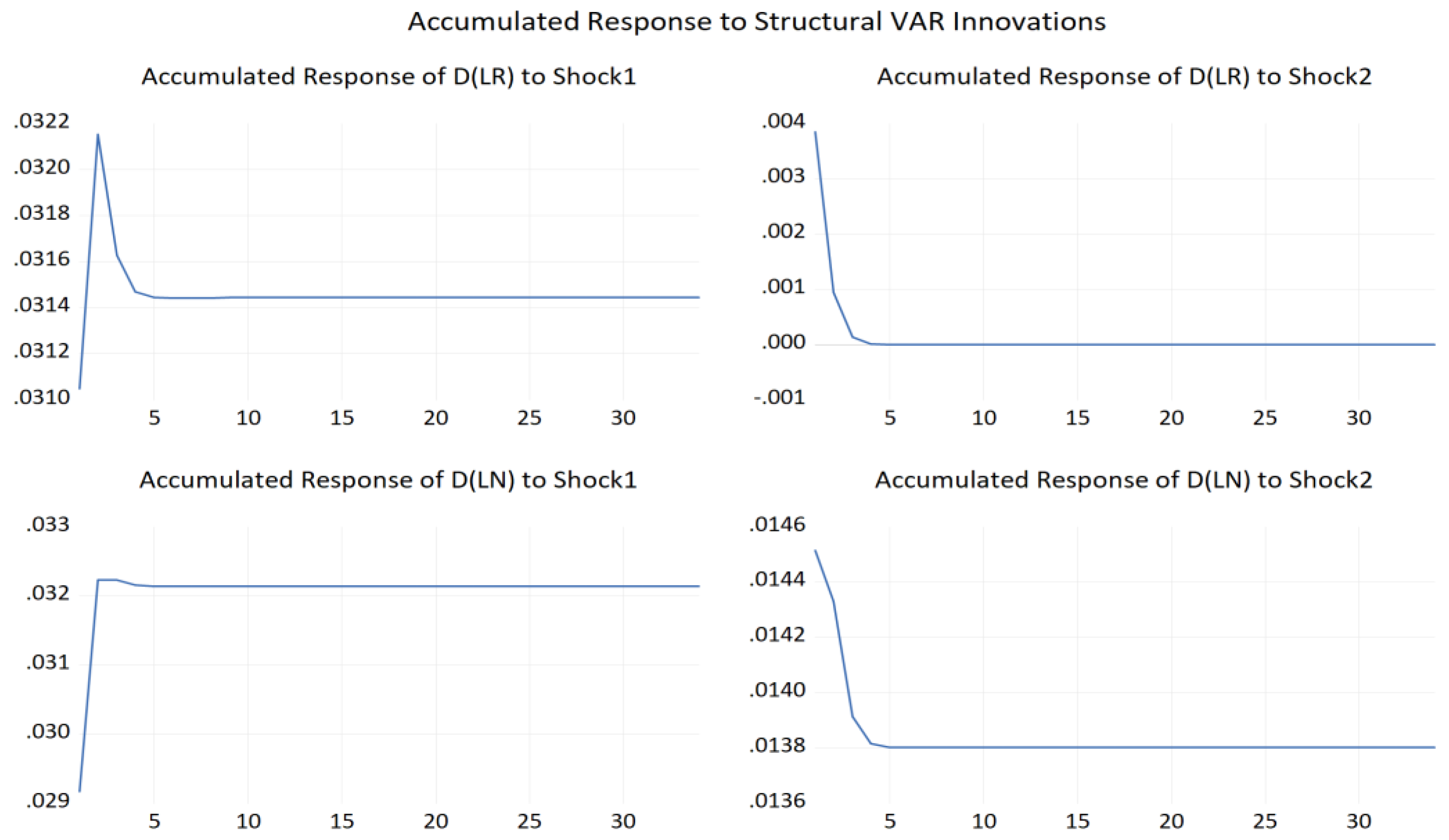
Figure 3.
Response of RER and NER to nominal and real shocks. Note: Figure 3 displays the accumulated response of real USDCAD (RER) and nominal USDCAD (NER) to real shocks (shock 1) and nominal shocks (shock 2).
Figure 3.
Response of RER and NER to nominal and real shocks. Note: Figure 3 displays the accumulated response of real USDCAD (RER) and nominal USDCAD (NER) to real shocks (shock 1) and nominal shocks (shock 2).
To complement the above analysis, variance decomposition analysis is included to analyze the impact of the real and nominal shocks on both real and nominal exchange rates. For brevity, Table 5 includes only the first 5 quarters. Consistent with earlier findings from Figure 3, nearly 98% of the variability in real CADUSD is explained by the real shocks, with the remaining 2% from nominal shocks. Similarly, for the nominal CADUSD, most of the variation (80%) is attributed to real shocks, with the remaining 20% attributed to nominal shocks.
5.4. Real and Nominal Shocks
While the above analysis support that real and nominal shocks have some discernable impact on the real and nominal USDCAD, the above analysis does not identify the real and nominal shocks as specific macroeconomic or financial variable. To this effect, we test, in line with existing literature review, for real shocks, using real government expenditure as a measure of demand shock and real GNP as a supply shocks. Money supply (M2) is used as a nominal shock. Impulse response analysis is carried out for each of the shock, from both Canada and US, on the NER and RER respectively, with results reported in Figure 4. Differenced log of real government expenditure and differenced log of real GNP were used as real demand and supply shocks, and nominal log of money supply (M2) was used as a measure of nominal shock. Accumulated responses for 30 first quarters following the shocks are reported, using the Cholesky (degree of freedom adjusted) decomposition method. All variables were stationary after first order differencing using ADF stationary test. Based on maximizing Schwarz, Hannan-Quinn, and Akaike information criteria, 1 lag & 4 lags were used in VAR models with US and Canadian shock variables respectively. A few observations can be made as follows.
First, both US and Canadian money supply have a marginal decrease on both the real and nominal USDCAD. A slower decay was noticed on the NER following a shock from the Canadian money supply. This is in line with earlier findings that nominal shocks have only a temporary effect on real and nominal exchange rate.
Secondly, supply shocks from real GNP from both countries resulted in a noticeable increase in the real and nominal USDCAD, before stabilizing at a higher rate after 5 quarters. This is consistent with earlier findings that real shocks have permanent effect on both NER and RER. A less significant response was observed on the NER following a shock from US real GNP, compared to a similar shock from the Canadian real GNP.
Results for the demand-side shocks were mixed. A shock from the Canadian's real government expenditure resulted in an increase and permanent impact on the RER. This is in line with earlier findings that real shocks cause a permanent effect on RER. Comparatively, a shock from Canadian's real government expenditure also resulted in an increase in the NER, before returning to its original state within 5 quarters.
Further, a shock from US real government expenditure resulted in lower NER and RER and stabilizing at a new rate after 5 quarters. Last, but not least, a self-shock resulted in an initial increase in the RER, before falling to stabilize at a lower but positive increase in the RER. This was also the case, for a self-shock in the RER in a system involving Canadian shocks. Comparatively, a self-shock resulted in an increase and permanent impact for NER, in a system involving US shocks. Although not reported here, self-shocks for both NER and RER contributed mostly to the variance decompositions of NER and RER.
6. Conclusive Remarks
Deglobalization and decarbonization are important drivers of inflation globally, and more particularly for countries like Canada and U.S. which are among the leading consumers, producers, and exporters of energy. COVID-19 can be attributed as a root cause of deglobalization, with a rise in volatility of prices in the last 4 years. After a decade, Canada has begun to witness sustained positive trade balances. Post COVID-19, both countries yielded real GDP which were increasing at a decreasing rate. While both economies’ wholesale price indices are positive correlated, the nominal exchange rate ranged between 0.7 U.S. dollar (USD) per Canadian dollar (CAD) to 0.8 U.S. during the period 2020-early 2024. Last, but not least, both exports and imports have been falling in 2023. With this backdrop of events, triggers and facts, this study sheds light on the long-run relationship between the Canadian dollar and U.S. dollar, by (i) showcasing that real shocks affect both the nominal and real exchange rate of USDCAD and that nominal shocks have only a temporary effect on the USDCAD; (ii) how real demand and supply shocks impact the nominal and real exchange rate, compared with a shock from nominal factors; (iii) how country-specific (US and Canada) factors affect the USDCAD in the long-run.
Both US and Canada are strong partners in trade, with their inflation policies (represented by WPIs), economic activity (real GNP) and monetary policy (money supply) measures being strongly positively linked with each other. Both economies' inflation measures were negatively correlated with the wholesale price ratio, with the higher WPI for Canada, leading to the real rate being lower than the nominal exchange rate. The nominal USDCAD was strongly negatively correlated with the wholesale price ratio. Although both countries share a strongest positive correlation in their money supplies, money supply from each country had a reduced effect on the wholesale price indices for each country, compared to real government expenditure and real GNP.
Accumulated responses of the real and nominal exchange rate to nominal and nominal shocks support that the effect from nominal shocks quickly vanishes. Conversely, the effect of real shocks on the nominal and real exchange rate between the Canadian dollar and US dollar is permanent. Specifically, although we observe a sudden increase for both NER and RER following a real shock, on one hand, the effect of the real shock overshoots before stabilizing at a higher than before RER. On the other hand, the effect of a real shock is a sudden and permanent increase. This result suggests that while real shocks have a more long-lasting effect on the nominal and real exchange rate, real shocks tend to lead to an overshooting in the short-run which however corrects itself as the market congregates to its new long-run equilibrium. Most of the variation in real (nominal) USDCAD is explained by real (nominal) shocks.
Using real government expenditure from Canada and US as demand factors; both countries’ real GNP as supply factors, and both nations’ nominal money supply as nominal factors, we carry an analysis of the response of these impulse on NER and RER. Both US and Canada’s money supply have an insignificant decrease in both real and nominal USDCAD. This is consistent with our earlier findings nominal shocks have only a temporary effect on real and nominal exchange rate. Supply shocks from both countries’ real GNP led to a rise in both real and nominal USDCAD, before stabilizing at a higher rate after 5 quarters. This is also aligned with earlier findings that real shocks have permanent effect on both NER and RER. A less significant response was detected on the NER following a shock from US real GNP, compared to a similar shock from Canada’s real GNP. Findings for demand-side factors were mixed. A shock from Canada’s real government expenditure led to a rise and permanent impact on the RER. This is consistent with earlier findings that real shocks cause a permanent effect on RER. Conversely, a shock from Canadian's real government expenditure also yielded a rise in the NER, before however returning to its original state within 5 quarters. Overall findings, support that real shocks have a permanent impact on both the real and nominal USDCAD exchange rate. Supply-side (real GNP) factors support this concluding remark more than demand-side (real government expenditure) factors, with nominal money supply barely impacting the long-run relationship between the U.S. dollar and Canadian dollar.
Overall, the results have some key policy implications can be summarized as follows. First, policy makers need to be aware that wholesale price indices in Canada are higher than those in the US. This is particularly important, as this result in real exchange rate being lower than its nominal counterpart. Monetary policy actors need to consider this price information when deciding how inflation across borders can affect trade between the two nations. Second, findings support, that real factors tend to affect nominal and real exchange rates permanently compared to nominal based factors such as money supply. It takes roughly five quarters for the effect to stabilize permanently. Specifically, real supply-side factors, in the form of real GNP, tend to be the advocate of a permanent shock on real and nominal exchange rate. Only Canada’s real government expenditure, as a demand-factor, tend to have a positive long-lasting impact on the USDCAD. This suggests that this news announcement from Canada plays a critical role in the relationship between the two North American currencies.
A future avenue of research can tap into exploring how this relationship cognates with other key partner countries as part of the de/globalized world, especially when it comes to the leading foreign currency pairs actively traded globally.
References
- Moulle-Berteaux, C. (2023). Global Multi-Asset Viewpoint: The Five Forces of Secular Inflation. Morgan Stanley Investment Management. https://www.morganstanley.com/im/publication/insights/articles/article_thefiveforcesofsecularinflation.pdf.
- Factset (2024). Investment Research. https://www.factset.com/solutions/investment-research.
- Chicago Mercantile Exchange Group. (2024). Crude oil futures and options. CME Group. https://www.cmegroup.com/markets/energy/crude-oil/light-sweet-crude.html.
- Gurrib, I.; Kamalov, F.; Starkova, O.; Makki, A.; Mirchandani, A.; & Gupta, N. (2023). Performance of Equity Investments in Sustainable Environmental Markets. Sustainability, 15(9), 7453. [CrossRef]
- Plotnick, A.R. (1963). Oil Imports: Protectionism Vs. National Security, Challenge, 11(6), 28-32. https://www.jstor.org/stable/40718665.
- Sánchez, J.J.G. (2023, August 16). American Protectionism: Can It Work? Epicenter At the Heart of Research and Ideas, Harvard University. https://epicenter.wcfia.harvard.edu/blog/american-protectionism-can-it-work.
- Lee, C.C., & Hussain, J. (2023). An assessment of socioeconomic indicators and energy consumption by considering green financing, Resources Policy, 81, Article 103374. [CrossRef]
- Sokhanvar, A., & Lee, C.-C. (2023). How do energy price hikes affect exchange rates during the war in Ukraine?. Empirical economics, 64(5), 2151-2164. [CrossRef]
- Natural Resources Canada (2023). Energy Factbook 2023-2024. https://energy-information.canada.ca/sites/default/files/2023-10/energy-factbook-2023-2024.pdf.
- International Energy Agency. (2022). Canada 2022: Energy Policy Review. https://www.iea.org/reports/canada-2022.
- Global Affairs Canada (2020, February 26). The Canada-United States-Mexico Agreement: Economic impact assessment. https://www.international.gc.ca/trade-commerce/assets/pdfs/agreements-accords/cusma-aceum/cusma-impact-repercussion-eng.pdf.
- Canadian Association of Petroleum Producers. (n.d.). Oil and Natural Gas in Canada. https://www.capp.ca/energy/canadas-energy-mix/.
- Government of Canada (2024). Coal facts. https://natural-resources.canada.ca/our-natural-resources/minerals-mining/mining-data-statistics-and-analysis/minerals-metals-facts/coal-facts/20071.
- Canada Nuclear Safety Commission (2023). Regulatory Action. https://www.cnsc-ccsn.gc.ca/eng/acts-and-regulations/regulatory-action/impala-canada-ltd/.
- Canada Action (2024). Environmental Leadership in Natural Resources. https://www.canadaaction.ca/climate_action.
- Kim, J. O. and Enders, W. (1991). Real and monetary causes of real exchange rate movements in the Pacific rim. Southern Economic Journal, 57, 1061-1070. [CrossRef]
- Baillie, R.T., & McMahon, P.C. (1989) The foreign exchange market: theory and econometric evidence. Cambridge: Cambridge University Press.
- Dibooglu, S. & Enders, W. (1995) Multiple cointegrating vectors and structural economic models: an application to the French Franc/US Dollar exchange rate. Southern Economic Journa, 61(4), 1098-1116. [CrossRef]
- Butt, S., Ramzan, M., Wong, W-K., Chohan, M. A., & Ramakrishnan, S. (2023). Unlocking the secrets of exchange rate determination in Malaysia: A Game-Changing hybrid model. Heliyon, 9, Article e19140. [CrossRef]
- Meese, R.A., & Rogoff, K. (1983). Empirical exchange rate models of the seventies: do they fit out of sample? Journal of International Economics, 14(1–2), 3–24. [CrossRef]
- Frankel, J.A., & Rose, A.K. (1995). Empirical research on nominal exchange rates, Handbook of International Economics, 3, 1689–1729. [CrossRef]
- Enders, W., & Lee, B.-S. (1997). Accounting for real and nominal exchange rate movements in the post-Bretton Woods period. Journal of International Money and Finance, 16(2), 233-254. [CrossRef]
- Blanchard, O.J., & Quah, D. (1988). The Dynamic Effects of Aggregate Demand and Supply Disturbances (Working paper No. 2737). National Bureau of Economic Research. https://www.nber.org/system/files/working_papers/w2737/w2737.pdf.
- Ji, Q., Shahzad, S. J. H., Bouri, E., & Suleman, M. T. (2020). Dynamic structural impacts of oil shocks on exchange rates: lessons to learn. Journal of Economic Structures, 9(20), 1-19. [CrossRef]
- Malik, F., & Umar, Z. (2019). Dynamic connectedness of oil price shocks and exchange rates. Energy Economics, 84, Article 104501. [CrossRef]
- Gurrib, I., & Kamalov, F. (2019). The implementation of an adjusted relative strength index model in foreign currency and energy markets of emerging and developed economies, Macroeconomics and Finance in Emerging Market Economies, 12(2), 105-123. [CrossRef]
- Jia, Y., Dong, Z., & An, H. (2023). Study of the modal evolution of the causal relationship between crude oil, gold, and dollar price series. International Journal of Energy Research, 2023, Article 7947434. [CrossRef]
- Dogru, T., Isik, C., & Sirakaya-Turk, E. (2019). The balance of trade and exchange rates: Theory and contemporary evidence from tourism. Tourism Management, 74, 12-23. [CrossRef]
- Avdjiev, S., Du, W., Koch, C., & Shin, H. S. (2019). The dollar, bank leverage, and deviations from covered interest parity. American Economic Review: Insights, 1(2), 193-208. [CrossRef]
- Bussière, M., Gaulier, G., & Steingress, W. (2020). Global trade flows: Revisiting the exchange rate elasticities. Open Economies Review, 31, 25-78. [CrossRef]
- Bruno, V., & Shin, H. S. (2023). Dollar and exports. The Review of Financial Studies, 36(8), 2963-2996. [CrossRef]
- Eichenbaum, M. S., Johannsen, B. K., & Rebelo, S. T. (2021). Monetary policy and the predictability of nominal exchange rates. The Review of Economic Studies, 88(1), 192-228. [CrossRef]
- Gründler, D., Mayer, E., & Scharler, J. (2023). Monetary policy announcements, information shocks, and exchange rate dynamics. Open Economies Review, 34(2), 341-369. [CrossRef]
- Gürkaynak, R. S., Kara, A. H., Kısacıkoğlu, B., & Lee, S. S. (2021). Monetary policy surprises and exchange rate behavior. Journal of International Economics, 130, Article 103443. [CrossRef]
- Bénétrix, A. S., & Lane, P. R. (2013). Fiscal shocks and the real exchange rate. 32nd issue of the International Journal of Central Banking. 1-32. https://www.ijcb.org/journal/ijcb13q3a1.htm.
- Hanif, W., Mensi, W., Alomari, M., & Andraz, J. M. (2023). Downside and upside risk spillovers between precious metals and currency markets: Evidence from before and during the COVID-19 crisis. Resources Policy, 81, Article 103350. [CrossRef]
- Sokhanvar, A., Çiftçioglu, S., & Lee, C.-C. (2023). The effect of energy price shocks on commodity currencies during the war in Ukraine, Resources Policy, 82, Article 103571. [CrossRef]
- Greenwood, R., Hanson, S.G., Stein, J. C., & Sunderam, A. (2023). A quantity-driven theory of term premia and exchange rates. The Quarterly Journal of Economics, 138(4), 2327-2389. [CrossRef]
- Fisher, L. A., & Huh, H.-S. (2002). Real exchange rates, trade balances and nominal shocks: evidence for the G-7. Journal of International Money and Finance, 21(4), 497-518. [CrossRef]
- Sarangi, P. K., Chawla, M., Ghosh, P., Singh, S., & Singh, P. K. (2022). FOREX trend analysis using machine learning techniques: INR vs USD currency exchange rate using ANN-GA hybrid approach. Materials Today: Proceedings, 49, 3170-3176. [CrossRef]
- Youssef, M., & Mokni, K. (2020). Modeling the relationship between oil and USD exchange rates: Evidence from a regime-switching-quantile regression approach. Journal of Multinational Financial Management, 55, Article 100625. [CrossRef]
- Adaramola, A. O., & Dada, O. (2020). Impact of inflation on economic growth: evidence from Nigeria. Investment Management & Financial Innovations, 17(2), 1-13. [CrossRef]
- Mussa, M. (1976). Adaptive and regressive expectations in a rational model of the inflationary process. Journal of Monetary Economics, 1(4), 423-442. [CrossRef]
- Frenkel, J. A. (1976). Inflation and the Formation of Expectations. Journal of Monetary Economics, 1(4), 403-421. [CrossRef]
- Zhou, S. (1995). The response of real exchange rates to various economic shocks. Southern Economic Journal, 936-954. [CrossRef]
- Sarno, L., & Taylor, M. P. (2001). Official intervention in the foreign exchange market: is it effective and, if so, how does it work?. Journal of Economic Literature, 39(3), 839-868. [CrossRef]
- Lane, P. R., & Milesi-Ferretti, G. M. (2007). The external wealth of nations mark II: Revised and extended estimates of foreign assets and liabilities, 1970–2004. Journal of international Economics, 73(2), 223-250. [CrossRef]
- Lavoie, M., & Seccareccia, M. (2006). The Bank of Canada and the modern view of central banking. International Journal of Political Economy, 35(1), 44-61. [CrossRef]
- Bouakez, H., & Eyquem, A. (2015). Government spending, monetary policy, and the real exchange rate. Journal of International Money and Finance, 56, 178-201. Get rights and content. [CrossRef]
- Gurrib, I., & Kamalov, F. (2022). Predicting bitcoin price movements using sentiment analysis: a machine learning approach. Studies in Economics and Finance, 39(3), 347-364. [CrossRef]
- Kamalov, F., Gurrib, I., & Rajab, K. (2021). Financial forecasting with machine learning: price vs return. Journal of Computer Science, 17(3), 251-264. [CrossRef]
- Kamalov, F., & Gurrib, I. (2022). Machine learning-based forecasting of significant daily returns in foreign exchange markets. International Journal of Business Intelligence and Data Mining, 21(4), 465-483. [CrossRef]
- Mao, Y., Chen, Z., Liu, S., & Li, Y. (2024). Unveiling the potential: Exploring the predictability of complex exchange rate trends. Engineering Applications of Artificial Intelligence, 133, Article 108112. [CrossRef]
- Arias, J. E., Rubio-Ramírez, J. F., & Waggoner, D. F. (2018). Inference based on structural vector autoregressions identified with sign and zero restrictions: Theory and applications. Econometrica, 86(2), 685-720. [CrossRef]
- Carriero, A., Clark, T. E., & Marcellino, M. (2019). Large Bayesian vector autoregressions with stochastic volatility and non-conjugate priors. Journal of Econometrics, 212(1), 137-154. [CrossRef]
- Kilian, L. (2013). Structural vector autoregressions. In N. Hashimzade & M. A. Thornton (Eds.),.
- Handbook of research methods and applications in empirical macroeconomics (pp. 515-554). Edward Elgar Publishing. [CrossRef]
- Baumeister, C., & Hamilton, J. D. (2019). Structural interpretation of vector autoregressions with incomplete identification: Revisiting the role of oil supply and demand shocks. American Economic Review, 109(5), 1873-1910. [CrossRef]
- Charfeddine, L., & Barkat, K. (2020). Short-and long-run asymmetric effect of oil prices and oil and gas revenues on the real GDP and economic diversification in oil-dependent economy. Energy Economics, 86, Article 104680. [CrossRef]
- Liu, D., Meng, L., & Wang, Y. (2020). Oil price shocks and Chinese economy revisited: New evidence from SVAR model with sign restrictions. International Review of Economics & Finance, 69, 20-32. [CrossRef]
- Yıldız, B. F., Hesami, S., Rjoub, H., & Wong, W. K. (2021). Interpretation of oil price shocks on macroeconomic Aggregates of South Africa: Evidence from SVAR. Journal of Contemporary Issues in Business and Government, 27(1), 279-287. https://cibgp.com/au/index.php/1323-6903/article/view/558/526.
- Suhendra, I., & Anwar, C. J. (2022). The response of asset prices to monetary policy shock in Indonesia: A structural VAR approach. Banks and Bank Systems, 17(1), 104-114. [CrossRef]
- Yilmazkuday, H. (2023). COVID-19 effects on the S&P 500 index. Applied Economics Letters, 30(1), 7-13. [CrossRef]
- Carrière-Swallow, Y., Magud, N.E., & Yépez, J.F. (2021). Exchange rate flexibility, the real exchange rate, and adjustment to terms-of-trade shocks. Review of International Economics; 29 (2): 439–483. [CrossRef]
- Kelesbayev, D., Myrzabekkyzy, K., Bolganbayev, A., & Baimaganbetov, S. (2022). The impact of oil prices on the stock market and real exchange rate: The case of Kazakhstan. International Journal of Energy Economics and Policy, 12(1), 163-168. https://www.econjournals.com/index.php/ijeep/article/view/11880/6201. [CrossRef]
- Ahmad, A. H., Pentecost, E. J., & Stack, M.M. (2023). Foreign aid, debt interest repayments and Dutch disease effects in a real exchange rate model for African countries. Economic Modelling, 126, Article 106434. [CrossRef]
- Demir, F., & Razmi, A. (2022). The real exchange rate and development theory, evidence, issues and challenges. Journal of Economic Surveys, 36(2), 386-428. [CrossRef]
- Gurrib, I. & F. Kamalov (2019). The implementation of an adjusted relative strength index model in foreign currency and energy markets of emerging and developed economies, Macroeconomics and Finance in Emerging Market Economies, 12:2, 105-123. [CrossRef]
- Bank for International Settlements (2022). Triennial Central Bank Survey. Bank of International Settlements. https://www.bis.org/statistics/rpfx22.htm.
- King, R.G., & Watson, M.W. (1992). Testing Long Run Neutrality., (Working paper No. 4156). National Bureau of Economic Research. [CrossRef]
- Huang, C. (2020, November, 20-22). Research on the linkage relationship between different levels of money supply and economic growth based on VAR model. 2020 2nd International Conference on Economic Management and Model Engineering (ICEMME), Chongqing, China. [CrossRef]
- Tan, E. C., Tang, C. F., & Palaniandi, R. D. (2022). What could cause a country’s GNP to be greater than its GDP?. The Singapore Economic Review, 67(02), 557-566. [CrossRef]
- Dornbusch, R. (1976). Expectations and exchange rate dynamics. Journal of political Economy, 84(6), 1161-1176. [CrossRef]
Figure 1.
Presence of Canadian dollar and USD in foreign currency trades. Note: Figure 1 reports the average daily turnover of Over-The-Counter (OTC) foreign exchange instruments for the Canadian dollar (CAD) and U.S. dollar (USD) for 2001-2022. Source: [68, author].
Figure 1.
Presence of Canadian dollar and USD in foreign currency trades. Note: Figure 1 reports the average daily turnover of Over-The-Counter (OTC) foreign exchange instruments for the Canadian dollar (CAD) and U.S. dollar (USD) for 2001-2022. Source: [68, author].
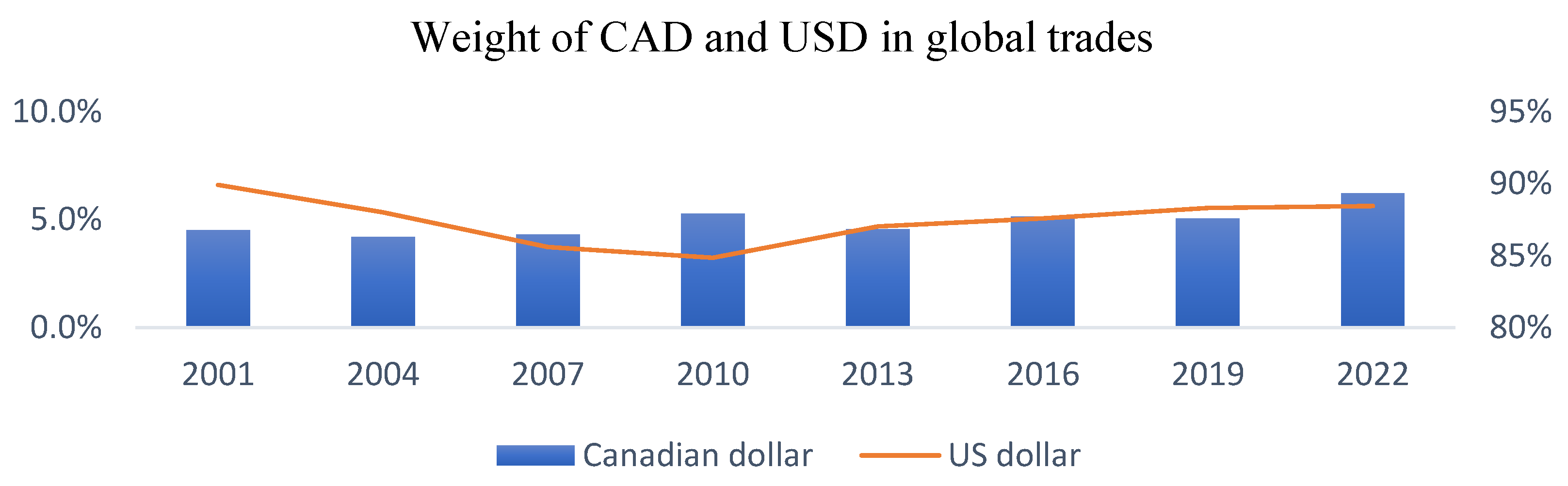
Figure 2.
NER and RER for Canada (Dec 1972-Dec 2023). Note: Figure 2 displays the nominal exchange rates (NER) and real exchange rates (RER) for Canada, using quarterly wholesale price ratios for the period December 1972- December 2023.
Figure 2.
NER and RER for Canada (Dec 1972-Dec 2023). Note: Figure 2 displays the nominal exchange rates (NER) and real exchange rates (RER) for Canada, using quarterly wholesale price ratios for the period December 1972- December 2023.
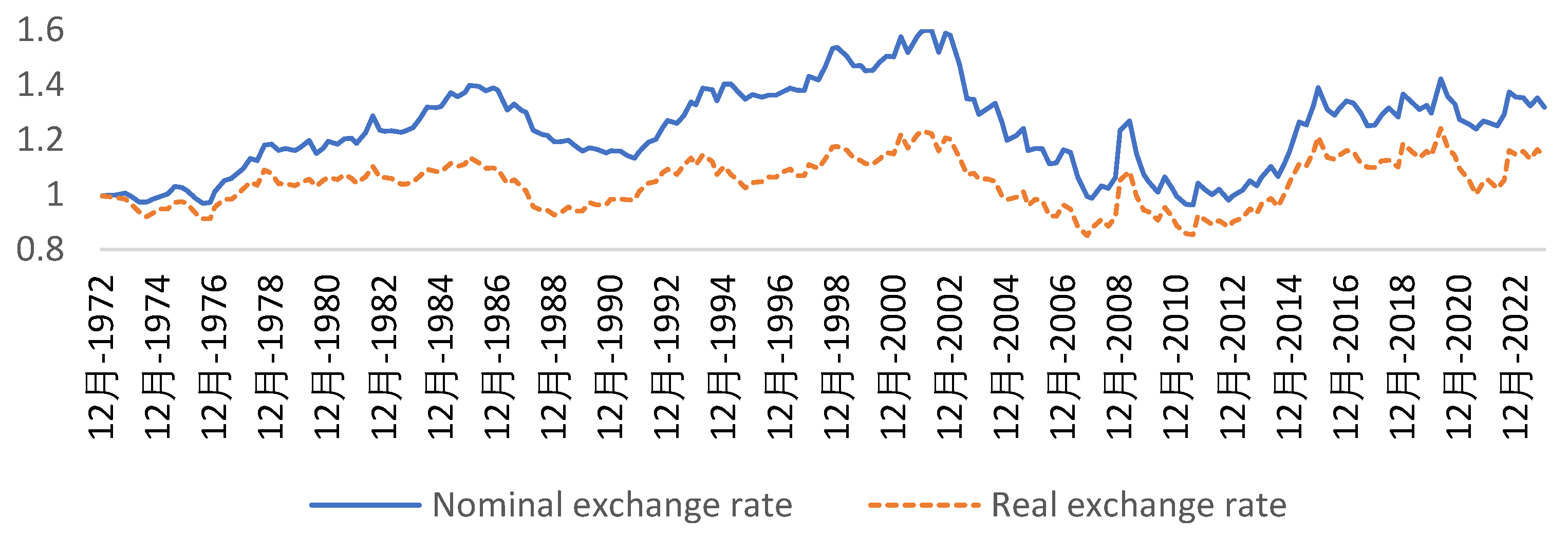
Figure 4.
Impulse responses of real and nominal shocks from US and Canada on NER and RER (December 1972 - December 2023). Note: Figure 4 displays the response of the real and nominal USDCAD to real and nominal shocks from Canada & US. Differenced log of real government expenditure and differenced log of real GNP were used as real demand and supply shocks, and money supply (M2) was used as a measure of nominal shock. Accumulated responses for 30 first quarters following the shocks are reported, using Cholesky (degree of adjusted) decomposition. All variables were stationary after first order differencing using ADF stationary test. Based on maximizing Schwarz, Hannan-Quinn, and Akaike information criteria, 1 lag & 4 lags were used in VAR models with US and Canadian shock variables respectively. Period of study is December 1972- December 202.
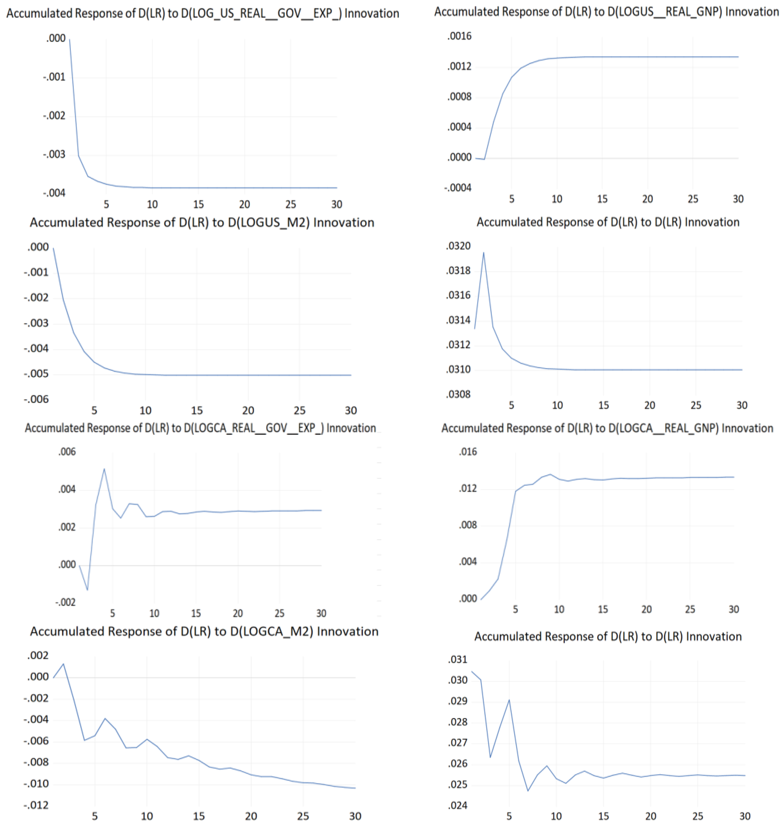
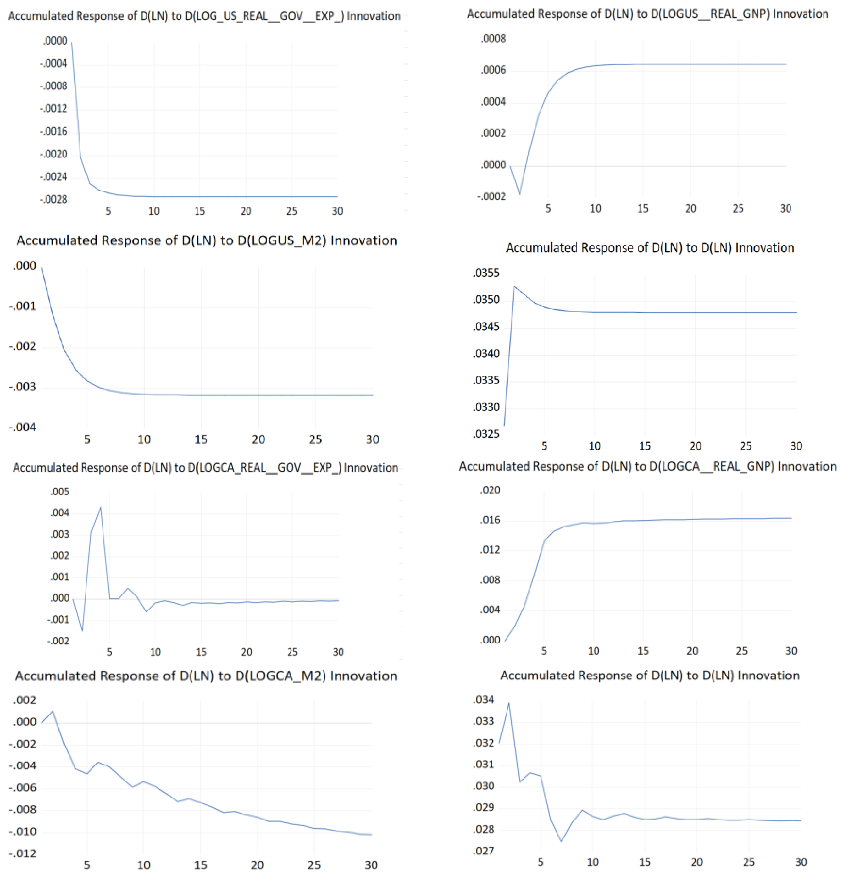
Table 1.
Descriptive Statistics.
| WPI_CA | WPI_US | Nominal USDCAD | Real USDCAD |
WPI-US/ WPI-CA |
||
|---|---|---|---|---|---|---|
| Mean | 391.678 | 330.030 | 1.237 | 1.043 | 0.849 | |
| Median | 401.115 | 310.709 | 1.244 | 1.052 | 0.856 | |
| Standard deviation | 142.439 | 121.213 | 0.158 | 0.088 | 0.057 | |
| Kurtosis | -0.331 | -0.602 | -0.650 | -0.783 | -0.549 | |
| Skewness | -0.049 | 0.190 | 0.083 | -0.075 | 0.250 | |
| Jarque-Bera | 1.019 | 4.319 | 3.843 | 5.427 | 4.713 | |
| p-value | 0.601 | 0.115 | 0.146 | 0.066 | 0.095 | |
| ADF | -0.358 | 0.244 | -0.1250 | -2.5970 | -2.6080 | |
| p-value | 0.9124 | 0.9747 | 0.2350 | 0.0953 | 0.0930 | |
| Observations | 205 | 205 | 205 | 205 | 205 | |
| US Real Gov. Exp. | CA Real Gov. Exp. | US Real GNP | CA Real GNP | US Money Supply |
CA Money Supply |
|
| Mean | 2,752 | 336 | 13.230 | 1.120 | 6,483.614 | 706.313 |
| Median | 2,709 | 313 | 12 | 0.905 | 4,184.100 | 449.658 |
| Standard deviation | 669 | 84 | 5 | 0.750 | 5,543.982 | 639.924 |
| Kurtosis | -1.267 | -0.864 | -1.265 | -0.766 | 0.765 | 0.639 |
| Skewness | -0.199 | 0.353 | 0.186 | 0.546 | 1.258 | 1.229 |
| Jarque-Bera | 15.068 | 10.634 | 14.853 | 15.187 | 59.052 | 55.070 |
| p-value | 0.001 | 0.005 | 0.001 | 0.001 | 0.000 | 0.000 |
| ADF | -0.4620 | 1.5730 | 1.4430 | 2.9980 | 2.7830 | 3.7530 |
| p-value | 0.8946 | 0.9995 | 0.9991 | 1.0000 | 1.0000 | 1.0000 |
| Observations | 205 | 205 | 205 | 205 | 205 | 205 |
Note: Table 1 summarizes the descriptive statistics for the US and Canadian wholesale price indices (WPI_US and WPI_CA), wholesale price ratio for USDCAD, nominal exchange rate (NER) and real exchange (RER) for the Canadian dollar relative to the US dollar (USDCAD), real government expenditures for US and Canada, and the real GNP and money supply for US and Canada. Real government expenditures, real Gross National Product (GNP) and money supply are in billion. M2 is used as the measure of money supply. 205 quarterly based observations are collected from Factset for December 1972-December 2023.
Table 2.
Correlation analysis.
| WPI_CA | WPI_US | Nominal USDCAD | Real USDCAD | WPI-US/WPI-CA | US Real Gov. Exp. | CA Real Gov. Exp. | US Real GNP | CA Real GNP | US Money supply | |
|---|---|---|---|---|---|---|---|---|---|---|
| WPI_US | 0.988 | 1.000 | ||||||||
| p-value | 0.000 | 0.000 | ||||||||
| Nominal USDCAD | 0.301 | 0.183 | 1.000 | |||||||
| p-value | 0.000 | 0.000 | 0.000 | |||||||
| Real USDCAD | 0.238 | 0.174 | 0.881 | 1.000 | ||||||
| p-value | 0.000 | 0.012 | 0.000 | 0.000 | ||||||
| WPI-US/WPI-CA | (0.328) | (0.187) | (0.795) | (0.421) | 1.000 | |||||
| p-value | 0.000 | 0.000 | 0.000 | 0.000 | 0.000 | |||||
| US Real Gov. Exp. | 0.957 | 0.955 | 0.196 | 0.130 | (0.256) | 1.000 | ||||
| p-value | 0.000 | 0.000 | 0.000 | 0.063 | 0.000 | 0.000 | ||||
| CA Real Gov. Exp. | 0.968 | 0.988 | 0.135 | 0.155 | (0.118) | 0.961 | 1.000 | |||
| p-value | 0.000 | 0.000 | 0.054 | 0.026 | 0.092 | 0.000 | 0.000 | |||
| US Real GNP | 0.965 | 0.975 | 0.184 | 0.187 | (0.159) | 0.973 | 0.982 | 1.000 | ||
| p-value | 0.000 | 0.000 | 0.000 | 0.000 | 0.022 | 0.000 | 0.000 | 0.000 | ||
| CA Real GNP | 0.962 | 0.982 | 0.133 | 0.169 | (0.089) | 0.945 | 0.991 | 0.988 | 1.000 | |
| p-value | 0.000 | 0.000 | 0.058 | 0.016 | 0.206 | 0.000 | 0.000 | 0.000 | 0.000 | |
| US Money supply | 0.905 | 0.930 | 0.123 | 0.216 | (0.013) | 0.857 | 0.952 | 0.928 | 0.966 | 1.000 |
| p-value | 0.000 | 0.000 | 0.078 | 0.000 | 0.855 | 0.000 | 0.000 | 0.000 | 0.000 | 0.000 |
| CA Money supply | 0.906 | 0.934 | 0.117 | 0.215 | (0.002) | 0.858 | 0.955 | 0.927 | 0.967 | 0.998 |
| p-value | 0.000 | 0.000 | 0.096 | 0.000 | 0.978 | 0.000 | 0.000 | 0.000 | 0.000 | 0.000 |
Table 5.
Variance decomposition (December 1972-December 2023).
| Variable | ∆RER | ∆RER | ∆NER | ∆NER |
| Shock | ||||
| 1-quarter | 98.489 | 1.511 | 80.153 | 19.847 |
| 3-quarters | 97.589 | 2.411 | 80.311 | 19.689 |
| 5-quarters | 97.588 | 2.412 | 80.311 | 19.689 |
| 7-quarters | 97.588 | 2.412 | 80.311 | 19.689 |
| 9-quarters | 97.588 | 2.412 | 80.311 | 19.689 |
Note: Table 5 represents the variance decomposition analysis of real and nominal shocks on ∆RER and ∆NER, where ∆RER (∆NER) is the first difference of real (nominal) Canadian dollar per US dollar. ( denotes the real (nominal) shocks. 5 quarters are reported. Values are in percentages.
Disclaimer/Publisher’s Note: The statements, opinions and data contained in all publications are solely those of the individual author(s) and contributor(s) and not of MDPI and/or the editor(s). MDPI and/or the editor(s) disclaim responsibility for any injury to people or property resulting from any ideas, methods, instructions or products referred to in the content. |
© 2024 by the authors. Licensee MDPI, Basel, Switzerland. This article is an open access article distributed under the terms and conditions of the Creative Commons Attribution (CC BY) license (http://creativecommons.org/licenses/by/4.0/).
Copyright: This open access article is published under a Creative Commons CC BY 4.0 license, which permit the free download, distribution, and reuse, provided that the author and preprint are cited in any reuse.


