Submitted:
24 July 2024
Posted:
25 July 2024
You are already at the latest version
Abstract
Photoplethysmography (PPG) signals, which measure blood volume changes through light absorption, are increasingly used for non-invasive Cardiovascular Disease (CVD) detection. Analyzing PPG signals can help identify irregular heart patterns and other indicators of CVD. This research involves a thorough analysis of CVD classification using the Capnobase dataset, which includes data from 20 CVD subjects and 21 normal subjects. In the initial stage, heuristic optimization algorithms, such as ABC-PSO, the Cuckoo Search algorithm (CSA), and the Dragonfly algorithm (DFA), were applied to reduce the dimension of the PPG data. Next, these Dimensionally Reduced (DR) PPG data are then fed into various classifiers such as Linear Regression(LR), Linear Regression with Bayesian Linear Discriminant Classifier (LR-BLDC), K-Nearest Neighbors (KNN), PCA-Firefly, Linear Discriminant Analysis (LDA), Kernel LDA (KLDA), Probabilistic LDA (ProbLDA), SVM-Linear, SVM-Polynomial, SVM-RBF, to identify CVD. Classifier performance is evaluated using Accuracy, Kappa, MCC, F1 Score, Good Detection Rate(GDR), Error rate, and Jaccard Index(JI). The SVM-RBF classifier for ABC PSO dimensionality reduced values outperforms other classifiers, achieving an accuracy of 95.12% with a MCC of 0.90.
Keywords:
CVD
; Dimensionality Reduction
; LR
; KNN
; LDA
; SVM
Introduction
Cardiovascular disease continues to be the leading cause of death globally, significantly burdening healthcare systems and economies. It accounts for approximately 17.9 million deaths annually, necessitating urgent advancements in prevention, diagnosis, and treatment strategies. Globally, life expectancy is on the rise due to significant advancements in healthcare, medicine, and a heightened awareness of personal hygiene and environmental hygiene [1]. Optimizing Computeraided diagnosis holds immense potential for healthcare. It fosters a more objective and consistent diagnostic approach, ultimately benefiting patient outcomes. Photoplethysmography (PPG) technology has the potential to revolutionize early detection of cardiovascular issues, aimed at increasing life expectancy and reducing healthcare costs [2,3]. It can be easily incorporated into wearable medical technology to measure various health-related metrics. Due to its diagnostic capabilities, PPG is widely utilized in clinical practices. Over the past decades, there has been a swift increase in the implementation of Wireless Patient Monitoring (WPM) and Internet of Things (IoT) models worldwide [4]. Cutting edge smart home automation and e-healthcare system technologies now enable in-home medical services, reducing the need for hospital visits [5]. Digital health has increasingly been integrated into daily life through digital health tools like smartwatches and health apps, facilitating real-time monitoring and diagnostics [6]. High blood pressure is a significant threat to developing cardiovascular diseases (CVDs) [7]. The World Health Organization (WHO) identifies cardiovascular disease as the leading chronic illness globally, significantly contributing to the overall disease burden and responsible for 31% of deaths worldwide [8]. PPG technology, highlighted as versatile and cost-effective [9], utilizes a photoelectric sensor to detect changes in light transmitted or reflected by blood vessels in the skin [10]. PPG does not require specific placement of sensors at predetermined locations on the body [11]; Measurements can be easily taken from the finger, wrist, or even earlobe [12]. This user-friendly approach makes PPG a popular biosignal for wearables, especially for monitoring heart rate during exercise and physical activity.
One of the most widely used technologies for monitoring a patient's physiological conditions is PPG. It is popular due to its non-invasive nature and low cost. Additionally, PPG's ability to provide continuous readings makes it ideal for use in pulse oximetry [13]. PPG signals require minimal hardware compared to traditional ECG monitoring systems, making them more accessible [14]. Shintomi et al. [15] investigated the effectiveness of compensating for heartbeat errors in mobile and wearable sensor data to improve heart rate variability (HRV) analysis. PPG sensors do not require a reference signal, making them ideal for integration into wristbands. This enhances their application, utility, and clinical applicability, making them highly effective for various research purposes in the analysis and diagnosis of CVD [16]. Moshawrab et al. [17] explored the use of smart wearable devices for detecting and predicting CVDs. The authors also reviewed the development and use of these wearables, which demonstrate their high effectiveness in managing CVDs. Reisner et al. [18] developed the use of the PPG for circulatory monitoring.
PPG signals are mostly preferred for CVD analysis because they are non-invasive and inexpensive while still offering valuable insights into blood flow variations that might indicate cardiovascular issues. Researchers have explored a diverse range of techniques for diagnosing CVD from PPG signals. Below are some of the notable works focusing on the exploration of PPG signals and their applications in various biomedical fields. Neha et al. [19] explored the use of PPG signals for arrhythmia detection. In this way, artifacts from the PPG signals are eliminated by employing the low-pass Butterworth filtering technique. After extracting informative features from the PPG data, machine learning algorithms were used to categorize pulses as normal or abnormal. Among the classifiers tested, SVM showed the strongest performance in identifying arrhythmic pulses, with an accuracy of 97.674%. Paradkar et al. [20] proposed a method for detecting coronary artery disease (CAD) by analyzing the characteristic points and temporal positions of the diastolic and systolic phases of PPG signals. Temporal features are extracted using Gaussian curve fitting, followed by singular value decomposition (SVD) and wavelet decomposition. Extracted temporal features are then fed to a SVM classifier to differentiate between individuals with coronary artery disease and healthy people. The proposed technique successfully classified CAD with a specificity of 78% and a sensitivity of 85%. Prabhakar et al. [21] proposed metaheuristic-based optimization algorithms to reduce the dimension of PPG signals obtained from the Capnobase dataset, and this dimensionality reduced PPG data is applied to different classifiers for CVD classification. Among the classifiers, the artificial neural network (ANN) achieved the highest classification accuracy of 99.48% for normal subjects when optimized with the chi-squared probability density function. On the other hand, the logistic regression classifier achieved the highest classification accuracy of 99.48% for CVD cases. Sivamani et al. [22] propose two different DR methods, such as heuristic and transformation based to reduce the dimension of the PPG signals and utilized twelve different classifiers to identify CVD using PPG data. The Hilbert transform DR method with the harmonic search classifier demonstrated superior performance, reaching an accuracy of 98.31% compared to other techniques. Rajaguru et al. [23] propose a method for cardiovascular disease detection based on statistical features extracted from PPG signals. Then the extracted features were classified using a linear regression classifier, resulting in an improved accuracy of 65.85%. Al Fahoum et al. (2024) presented a method for identifying cardiorespiratory disorders that utilizes PPG signals and classifiers that select the most relevant features through time-domain feature extraction. Data from 360 healthy individuals and CVD patients was analyzed, covering five types of CVD. The classification involved a cascade approach. Stage one performed a binary classification of healthy versus unhealthy subjects. Stage two focused on the unhealthy group, performing a multi-class classification to identify the specific disease type. Seven classifiers were tested, with the Naïve Bayes classifier achieving the maximum accuracy: 94.44% in the initial stage and 89.37% in the second stage. Prabhakar et al. (2025) leveraged a fuzzy-based approach to optimize parameters derived from PPG signals. These optimized features were then employed in a fuzzy model to predict cardiovascular disease (CVD) risk. The fuzzy model achieved its best performance when combined with Animal Migration Optimization (AMO) compared to four other optimization techniques. In this case, the SVM-RBF classifier achieved the highest accuracy of 95.05% in identifying CVD risk levels. Ihsan et al. [26] investigated methods for extracting informative features from PPG data to identify coronary heart disease. They focused on features capturing different aspects of the signal, including respiratory rate, heart rate variability, and other characteristics measured over time. Their approach using heart rate variability features achieved an accuracy of 94.4% in detecting coronary heart disease with a decision tree classifier. Liu et al. [27] classified the different heart rhythms from PPG signals by applying a deep convolutional neural network. They trained the system on PPG signals obtained from 45 patients, achieving an accuracy value of 85% in distinguishing multiple heart rhythms.
This research work makes the following key contributions:
- The study proposes an early detection and intervention method for cardiovascular diseases using PPG signals.
- Three metaheuristic optimization algorithms are used as DR techniques to reduce the dimension of the high-dimensional PPG data.
- The dimensionality-reduced PPG data was then analyzed using ten different classification algorithms to detect the presence of CVD. The classifiers' performance is evaluated using parameters such as accuracy, GDR, MCC, Kappa, error rate, F1 score, and Jaccard index.
The structure of this article is as follows: Section 1 presents the introduction, followed by the methodology in Section 2. Heuristic dimensionality reduction techniques are discussed in Section 3. Section 4 covers the ten different classifiers based on learning and selection parameters used to differentiate between normal and CVD-related segments within the PPG signal data. The findings of the work are thoroughly examined and interpreted in Section 5, and the conclusion of the work is provided in Section 6.
2. Materials and Methods
CVD analysis using PPG signals is crucial due to the rising prevalence of cardiovascular diseases globally. PPG technology offers a non-invasive, cost-effective, and easily deployable method for continuous heart health monitoring, facilitating early detection and timely intervention. This can reduce the burden on healthcare systems and improve patient outcomes. The integration of PPG analysis with wearable devices and advanced machine learning algorithms enhances diagnostic accuracy and efficiency. As healthcare shifts towards personalized and preventive models, PPG-based CVD analysis becomes a pivotal tool in the fight against CVDs. Therefore, CVD detection from PPG signals is considered in this research work. The main objective of this work is to enhance CVD diagnosis through more precise classification systems. Effectively categorizing CVD data not only ensures patients receive appropriate care at reduced costs but also lowers their risk of developing the disease. Classifier accuracy tends to decrease when unimportant and noisy signals are present in recorded signals. To enhance the quality of the recorded PPG signals, an efficient filtering technique is implemented to eliminate unwanted noise and artifacts. PPG data recordings with diverse wave shapes from the CapnoBase database have been used in this work. This database is a publicly available online resource that adheres to the IEEE TMBE pulse oximeter standard [25]. This article explores the CapnoBase dataset, utilizing the complete IEEE benchmark (41 records) for the experiment, with 20 records representing CVD and 21 representing normal conditions. The PPG signals are digitized at a rate of 200 samples per second. For analysis purposes, each one-second interval of the PPG signal is defined as a segment. Therefore, each patient has 720 individual segments for further examination. Consequently, each patient has 144,000 samples (720 segments × 200 samples per segment). The total number of CVD segments is [20 x 720 = 14400], and in normal cases, the total number of segments is [21 x 720 = 15120]. Therefore, in total, 29,520 one-second segments are available for analysis from the 41 cases. The PPG signals are analyzed based on signal segments across the patients. Beat-to-beat analysis is not included in this study. Noise components from the PPG signals were removed by utilizing Independent Component Analysis (ICA). Figure 1 shows a normal PPG signal, and Figure 2 depicts the PPG signal obtained from a CVD person.
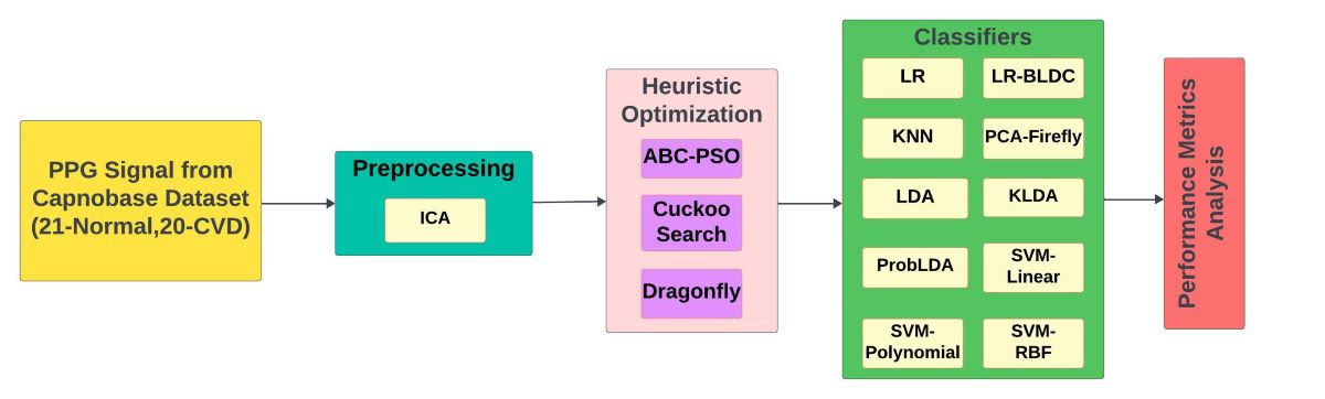
This research utilizes heuristic dimensionality reduction (DR) techniques as the initial step to reduce the dimensionality of the PPG data. Specifically, the research incorporates methods such as ABC-PSO (Artificial Bee Colony-Particle Swarm Optimization), the cuckoo search algorithm, and the dragonfly algorithm. In the second stage, the optimized PPG data were input into ten different classifiers to detect Cardiovascular disease from PPG signals. The classifiers' performance is evaluated and differentiated using parameter metrics for heuristically optimized PPG values. Figure 3 provides a detailed illustration of the workflow.
3. Dimensionality Reduction Techniques:
Now, each person has 144,000 samples of PPG signals (720 × 200). The objective of dimensionality reduction in PPG signals is to decrease the number of variables, thereby improving computational efficiency and reducing the risk of overfitting. High-dimensional data can be noisy and redundant, making it difficult for classifiers to accurately identify patterns associated with CVD. By extracting the most relevant features, dimensionality reduction techniques such as ABC-PSO, Cuckoo Search, and Dragonfly are employed to enhance the performance of machine learning models.
3.1. ABC-PSO (Artificial Bee Colony-Particle Swarm Optimization)
ABC-PSO is a hybrid dimensionality reduction technique that combines the global search capabilities of the ABC algorithm with the local exploitation abilities of Particle Swarm Optimization (PSO). ABC emphasizes exploration through employed and onlooker bees, where solutions are iteratively improved. PSO, inspired by social behavior, optimizes by updating particle velocities based on personal best and global best solutions. By integrating these approaches, the hybrid algorithm aims to enhance exploration-exploitation balance, leveraging ABC's local search capability and PSO's global search efficiency.This synergy enhances the efficiency of handling large datasets and improving the performance of data analysis[28].
ABC-PSO Algorithm Steps:
- Initialization: Initialize bee and particle populations with random solutions. Set the number of employed bees, onlooker bees, and scout bees, as well as particle positions and velocities
- Employed Bee Phase: Each employed bee explores new food sources (solutions) using:where is a random number and is a neighboring solution.
- Onlooker Bee Phase: Onlooker bees in the algorithm choose their food sources probabilistically:where is the fitness of solution
- Scout Bee Phase: Abandon poor solutions and have scout bees search for new random solutions.
- PSO Update: Update particle velocities and positions using:where is the personal best position, is the global best position, is the inertia weight, and are random numbers, and are acceleration coefficients.
- Evaluation and Selection: Evaluate new solutions and select the best ones based on fitness.
- Convergence Check: Repeat the steps until stopping criteria, such as maximum iterations or a convergence threshold are met.
3.2. Cuckoo Search Algorithm (CSA)
It is a nature-inspired metaheuristic optimization technique established by Xin-She Yang and Suash Deb in 2009[29]. Figure 4 illustrates the methodology of the CSA. It's effective for dimensionality reduction by finding optimal feature subsets. The feature subset is chosen that optimizes a performance metric, specifically aiming for the lowest MSE. This algorithm draws inspiration from the reproductive strategy of cuckoo birds. It simulates the unique behavior of cuckoos, which lay their eggs in the nests of other bird species. The algorithm employs both randomization and local search techniques to guide the cuckoos towards the optimal solution. A notable characteristic of CSA is its utilization of Levy flights, which are random walks characterized by a heavy-tailed distribution. This method regulates the movement of cuckoos, enabling efficient exploration of the feature space while swiftly navigating towards promising regions. Therefore, CSA is selected as a DR technique for its capability to balance exploration and exploitation and effectively manage high-dimensional data. The CSA commences its process by generating an initial population of cuckoos with random positions in the feature space. The position of each cuckoo in the population is then updated using the following equation.
Where, the cuckoo's previous position is represented by , while its updated position is denoted as .where α is a scaling factor, and Levy(λ) represents a step drawn from a Levy distribution.
The cuckoos' random search patterns are modeled by a concept called the Lévy flight, described by the following equation.
Here, '' represents the step size, is a parameter that dictates the scale of the Levy flight, and shape of the Levy flight is determined by the parameter μ. A random number chosen uniformly between 0 and 1. The optimal nest in the population is chosen based on the fitness value. MSE is used to derive the fitness value, and the best nest serves as the starting point for the next iteration of the algorithm. Also, abandon a fraction of the worst nests and generate new solutions to replace them. This process helps keep the search space varied, allowing the algorithm to explore new potential solutions. By using to periodically introduce new random solutions, the algorithm maintains a balance between exploration and exploitation, which is crucial for effective dimensionality reduction and optimization.
3.3. Dragonfly Algorithm
The Dragonfly Algorithm (DFA) is a heuristic optimization technique inspired by the fascinating static and dynamic swarming behaviors of dragonflies. DFA is developed by Seyedali Mirjalili in 2015[30], this algorithm mimics the way dragonflies search for food and avoid predators. Figure 5 presents the DFA flowchart. Dragonflies display two main behaviors: static, where they gather in small groups and hover around a target, and dynamic, where they collectively move towards a distant target. These behaviors are translated into mathematical models that help in exploring and exploiting the search space efficiently. It is effective for dimensionality reduction by finding optimal feature subsets through exploration and exploitation of the search space. As represented by Rahman et al. [31], separation, alignment, cohesion, attraction to food and distraction from the enemy are the important features of the DFA. In the following equations, represents the current positionof an individual dragonfly, denotes the position of the dragonfly, and ‘M’ indicates the total number of neighboring dragonflies.
Separation: It prevents dragonflies from crowding together by maintaining a minimum distance from each other.
The symbol represents the motion of separation exhibited by the individual.
Alignment: It refers to the tendency of dragonflies to match their velocity with that of their neighbors.
where represents the alignment motion for the individual, indicates neighboring individual dragon velocity.
Cohesion: is the behavior that drives dragonflies to move towards the center of their neighboring individuals.
Attraction: It is the tendency of dragonflies to move towards food sources
where represents the attraction of nutrition source for the individual flyand the position of the food source is denoted as .
Distraction: It is the tendency of dragonflies to move away from enemies.
where represents the distraction motion caused by the enemy for the individual and the location of the enemy is denoted as .
The positions of artificial dragonflies inside the designated search area are revised using the current position vector (q) and the step vector (∆q). The direction of their movement is determined by the step vector (∆q), and it is calculated as,
where iteration number is denoted as ‘t’, 'ω' denotes the inertia weight and weights assigned to separation, alignment, cohesion, attraction, and enemy, are denoted as s, a, c, f, and e respectively. The exploitation and exploration phases can be achieved by modifying the weights, once the step vector calculation is completed, calculation of the position vectors commences as below:
Statistical metrics such as Pearson correlation Coefficient (PCC), Sample Entropy, and Canonical Correlation Analysis (CCA), mean, variance, kurtosis, and skewness were employed to identify distinct characteristics in the PPG signals between the different classes, allowing for faster analysis as presented in Table 2.
It is perceived from the table 2 that the calculated mean values are notably lower for both normal and CVD cases under ABC PSO DR technique and also for cuckoo search normal category. For cuckoo search CVD class, a higher mean value is attained. Under dragon fly optimization, negative mean values are achieved for both Normal and CVD. Skewness and kurtosis values are considerably skewed for both normal and CVD for all three DR techniques. Table 2 indicates that the sample entropy values are same across classes with the exception of the cuckoo search DR technique in the CVD case. Table 2 further illustrates that the low PCC values suggest that the optimized features exhibit nonlinearity and lack correlation across different classes. If CCA values exceed 0.5, significant correlation between the classes can be expected. Table 2 shows that the dragon fly optimization is highly related to all of the classes compare to other DR techniques. It also shows that the ABC PSO DR technique has lower correlation with the other classes.
Figure 6 dipicts the histogram plot of ABC PSO DR values for normal person and it gives that the histogram with higher peaks in the middle and lower at either end. Figure 7 displays the histogram plot of ABC PSO DR values for CVD patient and it provides that the histogram isnormal and Gaussian nature.The scatter plot of ABC PSO DR values of normal and CVD data is depicted in Figure 8, which clearly indicates that the DR features are highly merged among the classes at the center and lesser overlapping at the end.The scatter plot of Dragon Fly DR values is portrayed in Figure 9. It shows that the lesser overlapping is present among the normal and CVD classes.
4. Classifiers for Classification of CVD from Dimensionality Reduced Values
4.1. Linear Regression as a Classifier
Linear regression(LR) falls under the category of supervised learning techniques. It is primarily employed to forecast continuous numerical outcomes. This algorithm establishes a linear relationship between input features and the target variable, allowing it to make predictions on new, unseen data based on the patterns learned from the training set. The linear equation is defined by a set of coefficients that are estimated using the training data. Linear regression is is primarily designed for predicting continuous numerical outcomes, it demonstrates versatility in its application. Through appropriate modifications, this algorithm can be effectively repurposed to address classification problems. The basic linear regression model is defined as[32]:
Where ,,…, are independent variables, is the dependent variable, is the intercept ,the coefficients are ,,…, and the error term is . For classification, the predicted values can be thresholded to determine class membership. In this research, we set a threshold of 0.5 to classify PPG data as either normal or CVD. Predictions greater than 0.5 are classified as CVD, while those less than 0.5 are considered normal. This approach is simple but can be limited by linear regression's assumptions and the nature of classification problems.
4.2. Linear Regression with BLDC
LR and LR-BLDC models use the same linear relationship, however LR is used for regression tasks with continuous outputs, whereas LR-BLDC adapts this relationship for binary classification by applying a threshold to the predicted values. The Bayesian Linear Discriminant Classifier operates as a probabilistic generative model specifically tailored for classification challenges. It involves estimating the class-conditional probability distribution of the input variables for each class and using Bayes' rule to calculate the posterior Probability of each class based on the input variables [33]. To combine linear regression and BLDC, the predicted output of the LR model as input to the BLDC model. The linear regression classifier output is used to estimate the mean of the class-conditional probability distribution for each class in the BLDC model.
4.3. K-Nearest Neighbor as a Classifier
The KNN algorithm compares the input point's distance to that of the K-nearest points in the training set. After identifying the K number of nearest neighbors, it allots the input point to the class with the maximum frequency among its K-nearest neighbors. It doesn't need a different phase for training. Instead, the algorithm retains the complete training dataset and employs it to classify new data points. Weighted KNN is a classification algorithm that assigns weights to the neighbors based on their distance to the query point. In the KNN algorithm, for a given point , the algorithm finds the K data points closest to a new point by measuring their distance using a metric like Euclidean distance. [34]:
In weighted KNN, each neighbor is assigned a weight inversely proportional to its distance from :
where is a small constant to avoid division by zero. The algorithm predicts the class of the query point by considering the most frequent class among its K closest neighbors:
where denotes the set of K nearest neighbors, the class label of neighbor is and the indicator function is I(⋅). This method improves the classification accuracy by giving more influence to closer neighbors.
4.4. PCA-Firefly
The hybrid PCA firefly technique is used to choose the most relevant features while removing irrelevant ones, thereby optimizing accuracy to its fullest extent. The PPG dataset undergoes dimensionality reduction using the PCA algorithm, which effectively reduces the quantity of stochastic variables to a concise group of primary variables. This approach greatly enhances the accuracy of the prediction results [35]. To further optimize the process, the firefly optimization algorithm is utilized to select the most appropriate attributes from this refined reduced dataset.
PCA simplifies data by finding a new set of features that are not related to each other by solving the eigenvalue problem:
where is the data matrix, are the eigenvectors (principal components), and λ are the eigenvalues.
The Firefly Algorithm is a clever problem-solving method that mimics how fireflies communicate with their flashes, optimizes the selection of principal components. Each firefly represents a potential solution with an intensity I proportional to its fitness. The attractiveness between fireflies and is given by:
where is the attractiveness at =0, is the light absorption coefficient, and is the distance between fireflies and . Fireflies are drawn to brighter ones, constantly adjusting their location:
where is a randomization parameter, and is a random vector. This process iteratively refines the feature selection, enhancing classification performance [36].
4.5. Linear Discriminant Analysis as a Classifier
Linear Discriminant Analysis (LDA) is a dimensionality reduction technique used for classification, aiming to find the best way to combine features to distinguish between different groups. LDA assumes that each class follows a Gaussian distribution with a shared covariance matrix. The steps of LDA involve [37]:
- Calculate the mean vector for each class
- Calculate the within-class scatter matrix
- Calculate the between-class scatter matrixWhere is the overall mean of the data set.
- Solve the generalized eigenvalue problem
The eigenvectors corresponding to the largest eigenvalues λ form the transformation matrix. Project the data onto this lower-dimensional space to maximize class separability. In classification, the new data point is projected and assigned to the class with the closest mean in this reduced space.
4.6. Kernel LDA as a Classifier
Kernel Linear Discriminant Analysis(KLDA) is an extension of LDA that incorporates the kernel trick to handle nonlinear data. The objective of this technique is to identify an optimal projection of the data in a high-dimensional feature space, which is created through the application of a kernel function. This projection is designed to simultaneously maximize the separation between different classes (between-class scatter) and minimize the spread within each individual class (within-class scatter).
The objective function of KLDA is formulated as:
where is the between-class scatter matrix and is the within-class scatter matrix in the kernel space. The solution corresponds to the eigenvector associated with the largest eigenvalue of the generalized eigenvalue problem .KLDA is effective for nonlinear data leveraging a kernel function to implicitly project the original input space into a higher-dimensional feature space, where data separation is potentially easier to achieve. It has found applications in various fields where nonlinear relationships among data features are prevalent [38].
4.7. Probabilistic LDA as a Classifier
Probabilistic Linear Discriminant Analysis (ProbLDA) is an extension of Linear Discriminant Analysis (LDA) that models class distributions probabilistically. ProbLDA assumes that each class follows a Gaussian distribution and utilizes Bayesian principles for classification [39]. The class mean, within-class scatter matrix and between-class scatter matrix are computed as per the equations 21,22 and 23.Then for each class Gaussian distributions can be assumed as follows:
Where is the Shared covariance matrix estimated as .
To calculate the posterior probabilities for classification, Bayes’ theorem can be used as per below equation.
Here ) prior probability of class and is the marginal probability of .Assign the new data point to the class with the highest posterior probability.
ProbLDA integrates the strengths of LDA with probabilistic modeling, providing a robust framework for classification.
4.8. Support Vector Machine as a Classifier
The Support Vector Machine (SVM) is a sophisticated supervised learning technique primarily employed for classification purposes. Its core principle involves identifying the most effective hyperplane that creates the widest possible margin between distinct classes within the feature space. It is used in the hyperplane to establish decision boundaries, distinguish between relevant and irrelevant vectors, and categorize data points into different classifications [40]. In SVM, input data is mapped to a higher-dimensional feature space using kernel functions to address multiclass classification problems. SVM aims to achieve high generalization by effectively separating classes based on the training data. Consider a binary classifier where a feature is associated with label‘h’ that belong to the set (−1,1). The classifier's decision is defined using parameters and b instead of the vector θ, the classification expression is,
Here K(y) =1 if y ≥ 0 and k(y)= -1 otherwise. The term ‘b’ is separated from other parameters using ‘z,b’. In this research, SVM with three different kernels are used: Radial Basis Function (RBF), linear, and polynomial [41].
SVM-Linear:
SVM-Polynomial:
where the degree of polynomial kernel is denoted as q and ‘ϒ’ denotes the gamma term in the kernel function.
SVM-RBF:
where, is Euclidean distance between two input vectors and .
These kernel functions operate by projecting the input data into a space of increased dimensionality. This transformation facilitates the identification of an optimal hyperplane that effectively delineates between different classes.
5. Results and Discussion
This research work employed a data partitioning strategy wherein 90% of the available dataset was dedicated to the model's training process, while the remaining 10% was set aside for subsequent testing and validation. To assess the classifier's efficacy and reliability, we implemented a ten-fold cross-validation approach. A True Positive (TP) occurs when the classifier correctly identifies a positive sample, while a True Negative (TN) is when it accurately labels a negative sample. A False Positive (FP) occurs when the model erroneously classifies a negative instance as positive, whereas a False Negative (FN) happens when the model incorrectly identifies a positive instance as negative. The Mean Squared Error (MSE) is defined by the following mathematical formula:
where M denotes the complete set of data points within the PPG dataset and it is assumed as 1000. The target value of model is designated by ,where the range of varies from 1 to 15; at a specific time, represents the observed value. The training was conducted in a manner that significantly reduced the classifier's Mean square error to a minimal value.
Table 3 presents the testing and training MSE for classifiers using three different DR techniques. The training MSE ranges from to , in contrast, the testing phase yielded MSE values ranging from to .The SVM-RBF classifier under the ABC-PSO dimensionality reduction method achieved the lowest training of 1.92 X and testing MSE value of 2.45 X . The DFA DR method yields somewhat reduced MSE values for both training and testing phases across the classifiers, when compared to the alternative DR approaches evaluated in this work. Similarly, for Cuckoo Search DR features the LR classifier yields the minimal testing MSE value of 1.37E-08, due the correct labelling of PPG signal for both CVD and normal subjects. The PCA Firefly classifier is plugged with a high number of FP and FN cases, resulting in the highest testing MSE of 6.08E-03. Similarly, for Dragon Fly DR values, the SVM-RBF classifier achieves the minimum testing Mean square error of 3.62E-09. This superior performance is attributed to its accurate labeling of PPG signals for both CVD and normal subjects. Conversely, the SVM-Linear classifier shows poorer performance, resulting in a much higher testing MSE of 9.03E-03. This higher error rate is due to the SVM-Linear misclassifying a significant number of cases, producing both false negatives and false positives.
5.1. Optimal Parameters Selection for Classifiers
When selecting the target values for the binary classification of PPG dataset (CVD and Normal class), a deliberate choice is made to assign the target ( values towards the upper end of the 0 to 1 range. The criteria used to select is as follows:
The complete set of CVD PPG data features, denoted as (Y), underwent a normalization process with mean . For the target values, a deliberate choice is made to assign them towards the lower end of the 0 to 1 range. The selection criteria for determining the value of are governed by the following parameters:
The complete set of normal PPG data features, denoted as (Y), underwent a normalization process with mean . For optimal categorization,
Based on the condition provided in (3), in this research work, the targets have been set at 0.1 for normal and 0.85 for CVD. Table 4 details the iterative process of selecting optimal parameters for the classifier during its training phase. A maximum of 1000 iterations is allowed to control the convergence criteria.
5.2. Performance Analysis of the Classifier
The classifiers' effectiveness is assessed using a comprehensive set of metrics, such as Accuracy, Good Detection Rate (GDR), F1 Score, Kappa, Matthews Correlation Coefficient (MCC), Error rate, and Jaccard Index. The following formula used for evaluating the overall effectiveness of the classification method.
Table 5 presents the results of the performance analysis for classifiers with three dimensionality reduction techniques. The results in Table 5 reveal that the classifier SVM-RBF for ABC PSO dimensionality reduction technique achieved very high scores on all benchmark metrics, including a superior accuracy of 95.12%, a F1 score and GDR of 95%, and a lowest error rate of 4.88%. Furthermore, the high Kappa and MCC are 0.90, with a Jaccard Index of 98.48%. The result demonstrates that the SVM-RBF classifier is outperforming for the ABC-PSO dimensionality reduction technique. Conversely, the KLDA classifier for the ABC-PSO dimensionality reduction method and the PCA-Firefly classifier for the Cuckoo Search dimensionality reduction technique demonstrated poor performance across all parameter values. This was evident from the lowest accuracy and F1 score of 53.66%, a GDR of 38.71%, and the highest error rate of 46.34%. Also, the low Kappa and MCC are 0.07, with a Jaccard Index of 36.67%. Upon analyzing individual dimensionality reduction techniques, the SVM (RBF) classifier performs better than other classifiers for the ABC-PSO DR technique, with a F1 score and GDR of 95% and a Jaccard Index of 98.48%. On the other hand, KLDA is the lowest performing classifier due to a higher error rate of 46.34% and reduced Kappa and MCC values of 0.07. Similarly, for the CSA DR method, the linear regression classifier achieved better accuracy at 90.24%, with a strong F1 score of 90% and a lower error rate of 9.76%. Meanwhile, for the Dragon Fly DR technique, the SVM-RBF classifier attained a higher accuracy of 92.68%, a GDR of 92.50%, and a high Matthews correlation coefficient of 0.85 due to a lower error rate of 7.32%.
Figure 10 illustrates the comparison of accuracy performance among classifiers using ABC PSO, Cuckoo Search, and Dragon Fly DR techniques.
Figure 10 presents the performance evaluation of classifiers across various DR techniques based on accuracy. Figure 10 reveals that the SVM-RBF classifier reigns supreme with an accuracy of 95.12%. Conversely, the KLDA classifier yields the lowest accuracy, at 53.66% for the ABC PSO DR method. Similarly, with CSA dimensionality reduced values, the LR classifier achieves the highest accuracy of 90.24%, while PCA-Firefly exhibits the lowest accuracy at 53.66%. The SVM-RBF classifier exhibited robust performance, achieving a notable accuracy of 92.68% when paired with the Dragonfly DR method. In contrast, the SVM with linear kernel struggled comparatively, yielding a considerably lower accuracy of 58.54%. Additionally, Figure 10 shows that the LR classifier performed well across all three DR techniques, achieving an accuracy of 90.24%.
Figure 11 shows that all classifiers using the three different DR techniques achieve an F1 score of around 60% or higher, indicating they are performing significantly better than random guessing. This indicates a notable alignment between the model's forecasts and the true class labels. It is also perceived that the maximum error rate observed is 46%, while the highest F1 score is 95%.
Figure 12 presents the histogram of accuracy and the Jaccard index for the classifiers. It is perceived that the maximum accuracy reaches 95%, while the highest Jaccard index is 90%. The accuracy histogram is left-skewed, indicating that the classifier's accuracy does not drop below 50% for any of the DR techniques. The Jaccard index histogram spans the entire spectrum, with values below 50% attributed to the classifiers' high false-positive rates.
5.3. Analysis of the Computational Complexity of Classifiers
Computational complexity is an important performance metric for classifiers. It is evaluated by considering the input size, denoted as . The computational complexity remains very low when the input size is . However, the computational complexity increases with the number of inputs. In this research, the computational complexity is independent of input size, which is a highly desirable characteristic for any algorithm. The term denotes the logarithmic rise in computational complexity with respect to .
The computational complexity of classifiers across different DR techniques is presented in Table 6. From table 6, the results clearly demonstrate that the SVM-RBF classifier has the highest computational complexity when used with the ABC-PSO and dragonfly DR techniques. Consequently, SVM-RBF achieves the highest accuracy, with 95.12% for the ABC-PSO dimensionality reduction technique and 92.68% for the dragonfly DR technique. Conversely, the KLDA classifier for the ABC-PSO dimensionality reduction technique and the PCA-Firefly classifier for the cuckoo search DR values produce the lowest accuracy of 53.66% while also having high computational complexity. This is attributed to their high false-positive rate and low Jaccard index.
As seen in Table 7, various machine learning classifiers, such as LR, NB, RBF NN, DCNN, KNN, DNN, ELM, ANN and SVM (RBF) have been utilized for classification of CVD from clinical database. The performance spectrum of these classifiers spans from a moderate 65% to an impressive 95% in terms of accuracy. However, this study specifically targets CVD detection using Capnobase dataset, with SVM (RBF) achieving the highest accuracy of 95.12%.
6. Conclusion
The main objective of this work is to classify PPG signals as either normal or indicative of cardiovascular disease. High-quality PPG samples were obtained by extracting useful features using heuristic-based DR methods such as ABC-PSO, Cuckoo Search, and Dragon Fly techniques. Ten classifiers were used for this purpose: LR, LR-BLDC, KNN, PCA-Firefly, LDA, KLDA, ProbLDA, SVM-Linear, SVM-Polynomial, and SVM-RBF. The SVM-RBF classifier, combined with the hybrid ABC-PSO dimensionality reduction technique, demonstrated superior performance. This approach achieved a remarkable accuracy of 95.12% while maintaining a minimal error rate of just 4.88%. Furthermore, it exhibited robust reliability, as evidenced by its high Matthews correlation coefficient and Kappa values, both reaching 0.90. Again, the second highest accuracy of 92.62% was achieved by the SVM-RBF classifier for Dragon Fly optimized values. The third highest accuracy of 90.24% was obtained by the LR classifier across all three DR techniques. Future research is focusing on convolutional neural networks (CNNs) and deep neural networks (DNNs) to swiftly detect cardiovascular disease.
References
- Centers for Disease Control and Prevention. The State of Aging and Health in America 2013; Centers for Disease Control and Prevention, US Department of Health and Human Services: Atlanta, GA, USA, 2013. [Google Scholar]
- Kranjec, J, Beguš, S, Geršak, G & Drnovšek, J 2014, ‘Non-contact heart rate and heart rate variability measurements: A review’, Biomedical signal processing and control, vol.13, pp.102-112.
- Miranda, E, Irwansyah, E, Amelga, AY, Maribondang, MM & Salim, M 2016, ‘Detection of cardiovascular disease risk's level for adults using naive Bayes classifier’, Healthcare informatics research, vol.22, no.3, pp.196.
- Majumder S., Mondal T., and Deen M. J., Wearable sensors for remote health monitoring, Sensors. (2017) 17, no. 12, https://doi.org/10.3390/s17010130, 2-s2.0-85009999439. [CrossRef]
- Manogaran G., Shakeel P. M., Fouad H., Nam Y., Baskar S., Chilamkurti N., and Sundarasekar R., Wearable IoT smart-log patch: an edge computing-based bayesian deep learning network system for multi access physical monitoring system, Sensors. (2019) 19, no. 13, https://doi.org/10.3390/s19133030, 2-s2.0-85070464464. [CrossRef]
- Norgeot B., Glicksberg B. S., and Butte A. J., A call for deep-learning healthcare, Nature Medicine. (2019) 25, no. 1, 14–15. [CrossRef]
- Al-Zaben A., Fora M., and Obaidat A., Detection of premature ventricular beats from arterial blood pressure signal, Proceedings of the 2018 IEEE 4th Middle East Conference on Biomedical Engineering (MECBME), 28-30 March 2018, Tunis, Tunisia, IEEE, 17–19.
- Hindia M. N., Rahman T. A., Ojukwu H., Hanafi E. B., and Fattouh A., Enabling remote health-caring utilizing iot concept over LTE-femtocell networks, PLoS One. (2016) 11, no. 5, e0155077, https://doi.org/10.1371/journal.pone.0155077, 2-s2.0-84968677659. [CrossRef]
- Savkar A., Khatate P., and Patil C., Study on techniques involved in tourniqueteless blood pressure measurement using PPG, Proceedings of the 2018 Second International Conference on Intelligent Computing and Control Systems (ICICCS), 14-15 June 2018, Madurai, India, IEEE, 170–172.
- Elgendi M., Fletcher R., Liang Y., Howard N., Lovell N. H., Abbott D., Lim K., and Ward R., The use of photoplethysmography for assessing hypertension, NPJ digital medicine. (2019) 2, no. 1, https://doi.org/10.1038/s41746-019-0136-7. [CrossRef]
- Allen J., Photoplethysmography and its application in clinical physiological measurement, Physiological Measurement. (2007) 28, no. 3, R1–R39, https://doi.org/10.1088/0967-3334/28/3/r01, 2-s2.0-34247467602. [CrossRef]
- Gu-Young J., Yu K.-H., and Nam-Gyun K., Continuous blood pressure monitoring using pulse wave transit time, Proceedings of the ICCAS 2005 International conference on Control, June 2-5, Gyeonggi-Do, Korea, Automation and systems, 834–837.
- Shin, H.; Min, S. Feasibility study for the non-invasive blood pressure estimation based on ppg morphology: normotensive subject study. Biomed. Eng. Online 2017, 16, 10. [Google Scholar] [CrossRef] [PubMed]
- J.L. Moraes, M.X. Rocha, G.G.Vasconcelos, J.E. Vasconcelos Filho, de Albuquerque V.H.C. de Albuquerque, A.R. Alexandria, Advances in photopletysmography signal analysis for biomedical applications, Sensors 18(6) (2018) 1–26. [CrossRef]
- Shintomi, A.; Izumi, S.; Yoshimoto, M.; Kawaguchi, H. Effectiveness of the heartbeat interval error and compensation method on heart rate variability analysis. Healthc. Technol. Lett. 2022, 9, 9–15. [Google Scholar] [CrossRef] [PubMed]
- Rubins, U. Finger and ear photoplethysmogram waveform analysis by fitting with Gaussians. Med Biol. Eng. 2008, 46, 1271–1276. [Google Scholar] [CrossRef] [PubMed]
- Moshawrab, M.; Adda, M.; Bouzouane, A.; Ibrahim, H.; Raad, A. Smart Wearables for the Detection of Cardiovascular Diseases: A Systematic Literature Review. Sensors 2023, 23, 828. [Google Scholar] [CrossRef] [PubMed]
- Reisner, A., Shaltis, P.A., McCombie, D., Asada, H.H. (2008). Utility of the photoplethysmogram in circulatory monitoring. Anesthesiology, 108 (5), 950- 958.
- Neha; Kanawade, R.; Tewary, S.; Sardana, H.K. Photoplethysmography based arrhythmia detection and classification. In Proceedings of the 6th International Conference on Signal Processing and Integrated Networks (SPIN), Noida, India, 7–8 March 2019; pp. 944–948. [CrossRef]
- Paradkar, N.; Chowdhury, S.R. Coronary artery disease detection using photoplethysmography. In Proceedings of the 39th Annual International Conference of the IEEE Engineering in Medicine and Biology Society (EMBC), Jeju, Republic of Korea, 11–15 July 2017; pp. 100–103. [Google Scholar] [CrossRef]
- Prabhakar, S.K.; Rajaguru, H.; Lee, S.W. Metaheuristic-based dimensionality reduction and classification analysis of PPG signals for interpreting cardiovascular disease. IEEE Access 2019, 7, 165181–165206. [Google Scholar] [CrossRef]
- Palanisamy, Sivamani, and Harikumar Rajaguru. "Machine learning techniques for the performance enhancement of multiple classifiers in the detection of cardiovascular disease from PPG signals." Bioengineering 10.6 (2023): 678.
- Rajaguru, H.; Shankar, M.G.; Nanthakumar, S.P.; Murugan, I.A. Performance analysis of classifiers in detection of CVD using PPG signals. In AIP Conference Proceedings; AIP Publishing LLC: Melville, NY, USA, 2023; Volume 2725, p. 020002. [Google Scholar] [CrossRef]
- Al Fahoum, A.S.; Abu Al-Haija, A.O.; Alshraideh, H.A. Identification of Coronary Artery Diseases Using Photoplethysmography Signals and Practical Feature Selection Process. Bioengineering 2023, 10, 249. [Google Scholar] [CrossRef] [PubMed]
- Prabhakar, S.K.; Rajaguru, H.; Kim, S.H. Fuzzy-inspired photoplethysmography signal classification with bioinspired optimization for analyzing cardiovascular disorders. Diagnostics 2020, 10, 763. [Google Scholar] [CrossRef] [PubMed]
- Ihsan, M.F.; Mandala, S.; Pramudyo, M. Study of Feature Extraction Algorithms on Photoplethysmography (PPG) Signals to Detect Coronary Heart Disease. In Proceedings of the International Conference on Data Science and Its Applications (ICoDSA), Bandung, Indonesia, 6–7 July 2022; pp. 300–304. [Google Scholar] [CrossRef]
- Liu, Z.; Zhou, B.; Jiang, Z.; Chen, X.; Li, Y.; Tang, M.; Miao, F. Multiclass Arrhythmia Detection and Classification from Photoplethysmography Signals Using a Deep Convolutional Neural Network. J. Am. Heart Assoc. 2022, 11, e023555. [Google Scholar] [CrossRef] [PubMed]
- Limon, M. F. A., Shiblee, M. F. H., Rouf, A., & Iqbal, M. S. (2023, December). Hybrid ABC-PSO Algorithm based Static Synchronous Compensator for Enhancing Power System Stability. In 2023 10th IEEE International Conference on Power Systems (ICPS) (pp. 1-6). IEEE.
- Yang, Xin-She, and Suash Deb. "Cuckoo search via Lévy flights." In 2009 World congress on nature & biologically inspired computing (NaBIC), pp. 210-214. Ieee, 2009.
- Mirjalili, S. Dragonfly algorithm: A new meta-heuristic optimization technique for solving single-objective, discrete, and multi-objective problems. Neural Comput. Appl. 2016, 27, 1053–1073. [Google Scholar] [CrossRef]
- Rahman, C. M., & Rashid, T. A. (2019). Dragonfly algorithm and its applications in applied science survey. Computational Intelligence and Neuroscience, 2019(1), 9293617.
- Hasan, M. A., Hasan, M. K., & Mottalib, M. A. (2015). Linear regression–based feature selection for microarray data classification. International journal of data mining and bioinformatics, 11(2), 167-179.
- Zhou W, Liu Y, Yuan Q, Li X,2013, ‘Epileptic seizure detection using lacunarity and Bayesian linear discriminant analysis in intracranial EEG. IEEE Transactions on Biomedical Engineering, vol. 60, no. 12, pp. 3375-3381.
- Pandey, A., & Jain, A. (2017). Comparative analysis of KNN algorithm using various normalization techniques. International Journal of Computer Network and Information Security, 10(11), 36. Pandey, A., & Jain, A. (2017). Comparative analysis of KNN algorithm using various normalization techniques. International Journal of Computer Network and Information Security, 10(11), 36.
- Granato, D, Santos, JS,Escher, GB, Ferreira, BL & Maggio, RM 2018,‘Use of principal component analysis (PCA) and hierarchical cluster analysis (HCA) for multivariate association between bioactive compounds and functional properties in foods: A critical perspective’, Trends in Food Science & Technology,vol. 72, pp. 83-90.
- Moazenzadeh, R, Mohammadi, B, Shamshirband, S & Chau, KW 2018, ‘Coupling a firefly algorithm with support vector regression to predict evaporation in northern Iran’, Engineering Applications of Computational Fluid Mechanics, vol. 12, no. 1, pp. 584-597.
- Zhao, H., Lai, Z., Leung, H., Zhang, X. (2020). Linear Discriminant Analysis. In: Feature Learning and Understanding. Information Fusion and Data Science. Springer, Cham. [CrossRef]
- Li, S., Zhang, H., Ma, R., Zhou, J., Wen, J., & Zhang, B. (2023). Linear discriminant analysis with generalized kernel constraint for robust image classification. Pattern Recognition, 136, 109196.
- Ioffe, S. (2006). Probabilistic Linear Discriminant Analysis. In: Leonardis, A., Bischof, H., Pinz, A. (eds) Computer Vision – ECCV 2006. ECCV 2006. Lecture Notes in Computer Science, vol 3954. Springer, Berlin, Heidelberg. [CrossRef]
- Srunitha, K & Padmavathi, S 2016, ‘Performance of SVM classifier for image based soil classification’, In 2016 International Conference on Signal Processing, Communication, Power and Embedded System (SCOPES), pp. 411-415, IEEE.
- Ramamoorthy, K.; Rajaguru, H. Exploitation of Bio-Inspired Classifiers for Performance Enhancement in Liver Cirrhosis Detection from Ultrasonic Images. Biomimetics 2024, 9, 356. [Google Scholar] [CrossRef] [PubMed]
- Hosseini, Z.S.; Zahedi, E.; Attar, H.M.; Fakhrzadeh, H.; Parsafar, M.H. Discrimination between different degrees of coronary artery disease using time-domain features of the finger photoplethysmogram in response to reactive hyperemia. Biomed. Signal Process. Control 2015, 18, 282–292. [Google Scholar] [CrossRef]
- Miao, K.H.; Miao, J.H. Coronary heart disease diagnosis using deep neural networks. Int. J. Adv. Comput. Sci. Appl. 2018, 9, 1–8. [Google Scholar] [CrossRef]
- Shobitha, S.; Sandhya, R.; Ali, M.A. Recognizing cardiovascular risk from photoplethysmogram signals using ELM. In Pro-ceedings of the Second International Conference on Cognitive Computing and Information Processing (CCIP), Mysore, In-dia, 12–13 August 2016; pp. 1–5. [CrossRef]
- Soltane, M.; Ismail, M.; Rashid, Z.A. Artificial Neural Networks (ANN) approach to PPG signal classification. Int. J. Comput. Inf. Sci. 2004, 2, 58–65. [Google Scholar]
Figure 1.
PPG signals for Normal Subject.
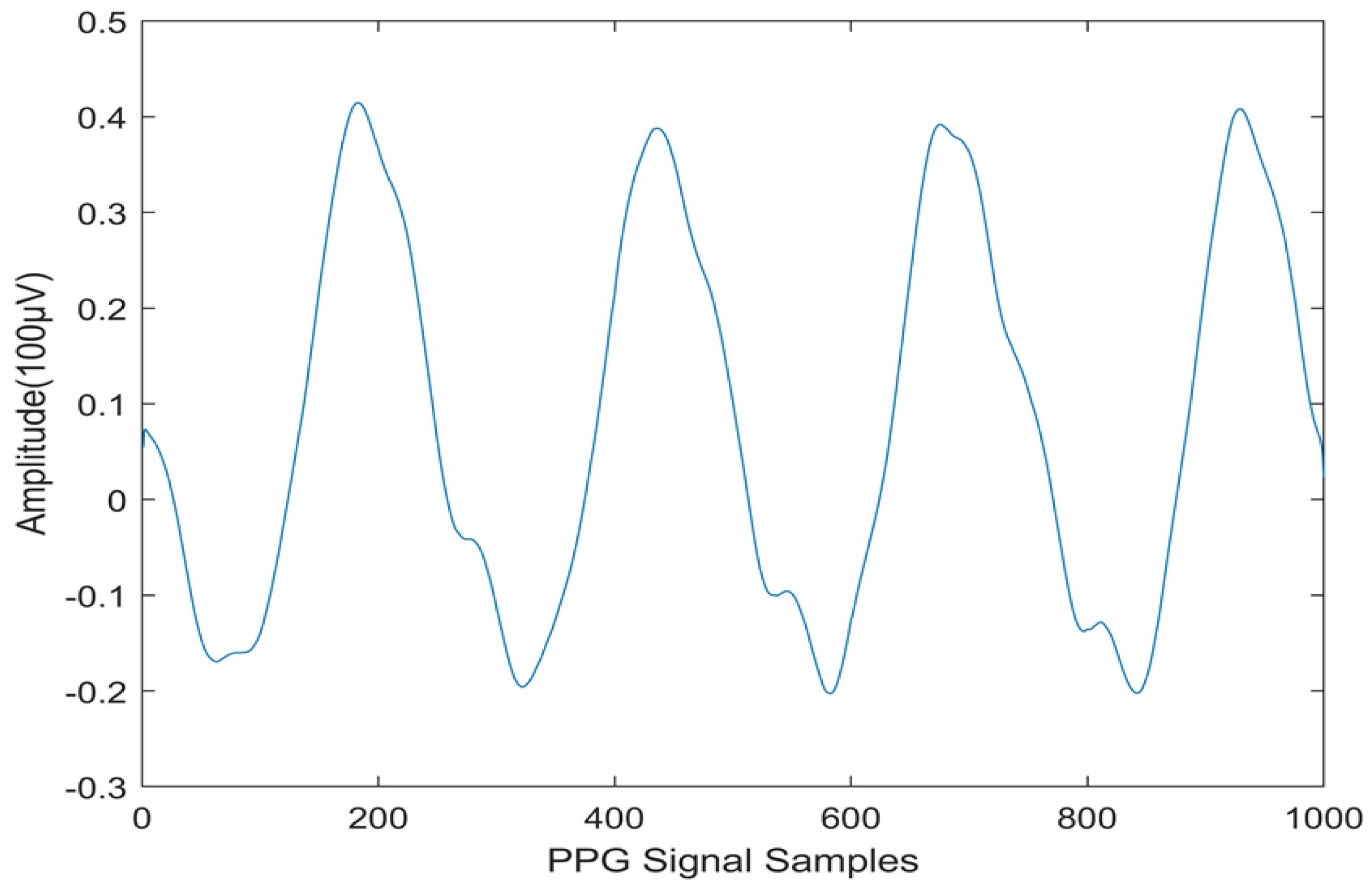
Figure 2.
PPG signals for CVD Subject.
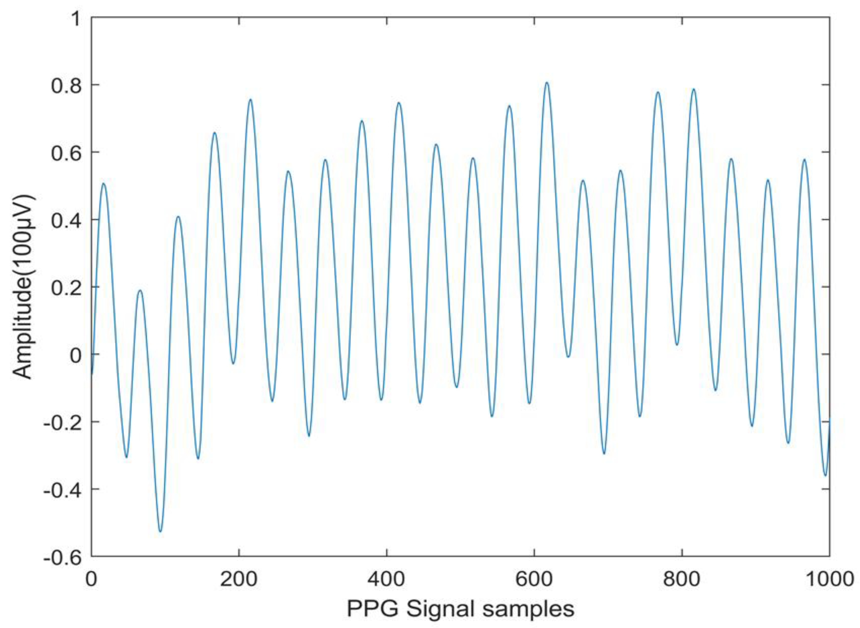
Figure 3.
Detailed illustration of the workflow.
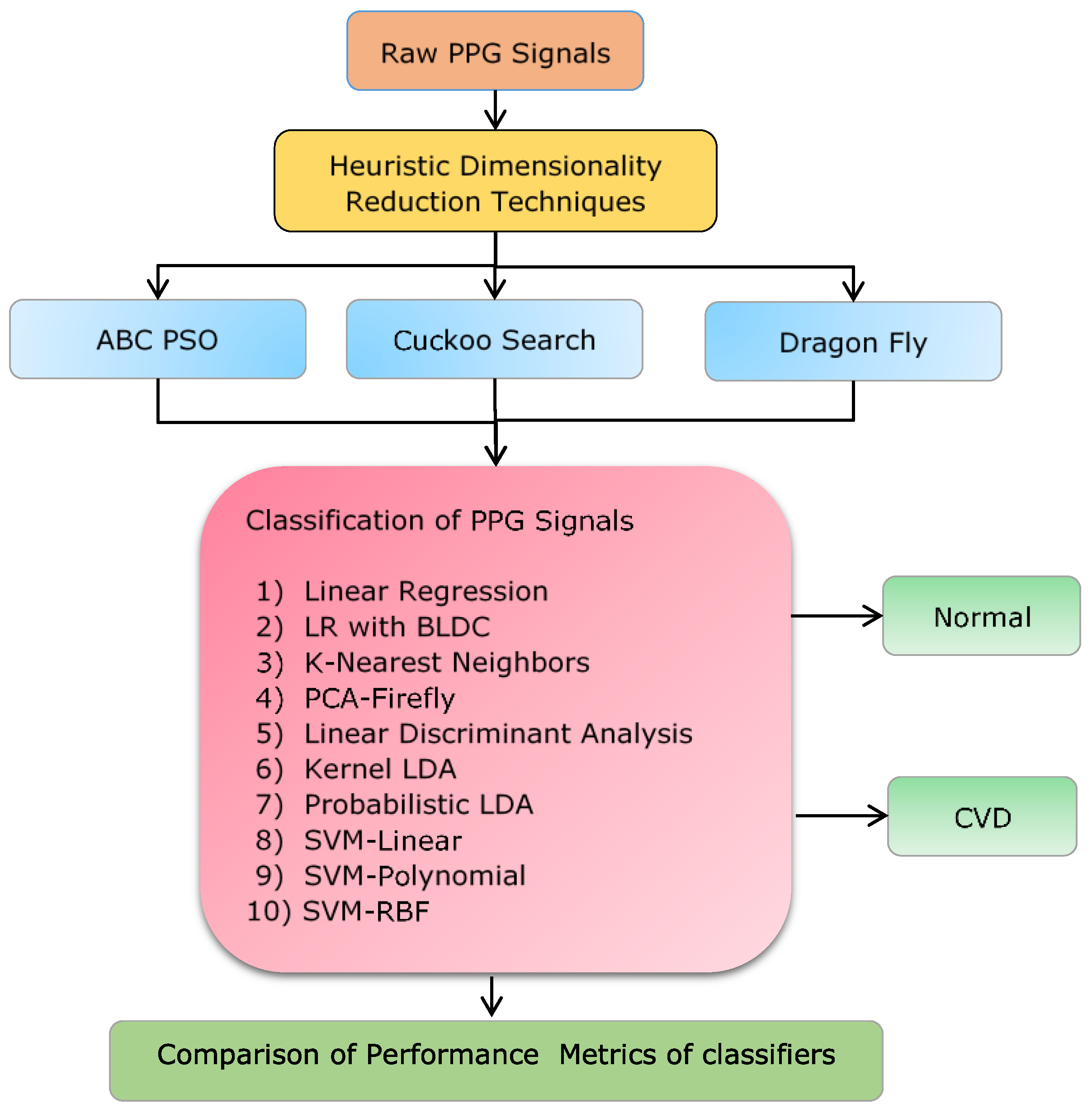
Figure 4.
Flowchart of the Cuckoo Search Algorithm.
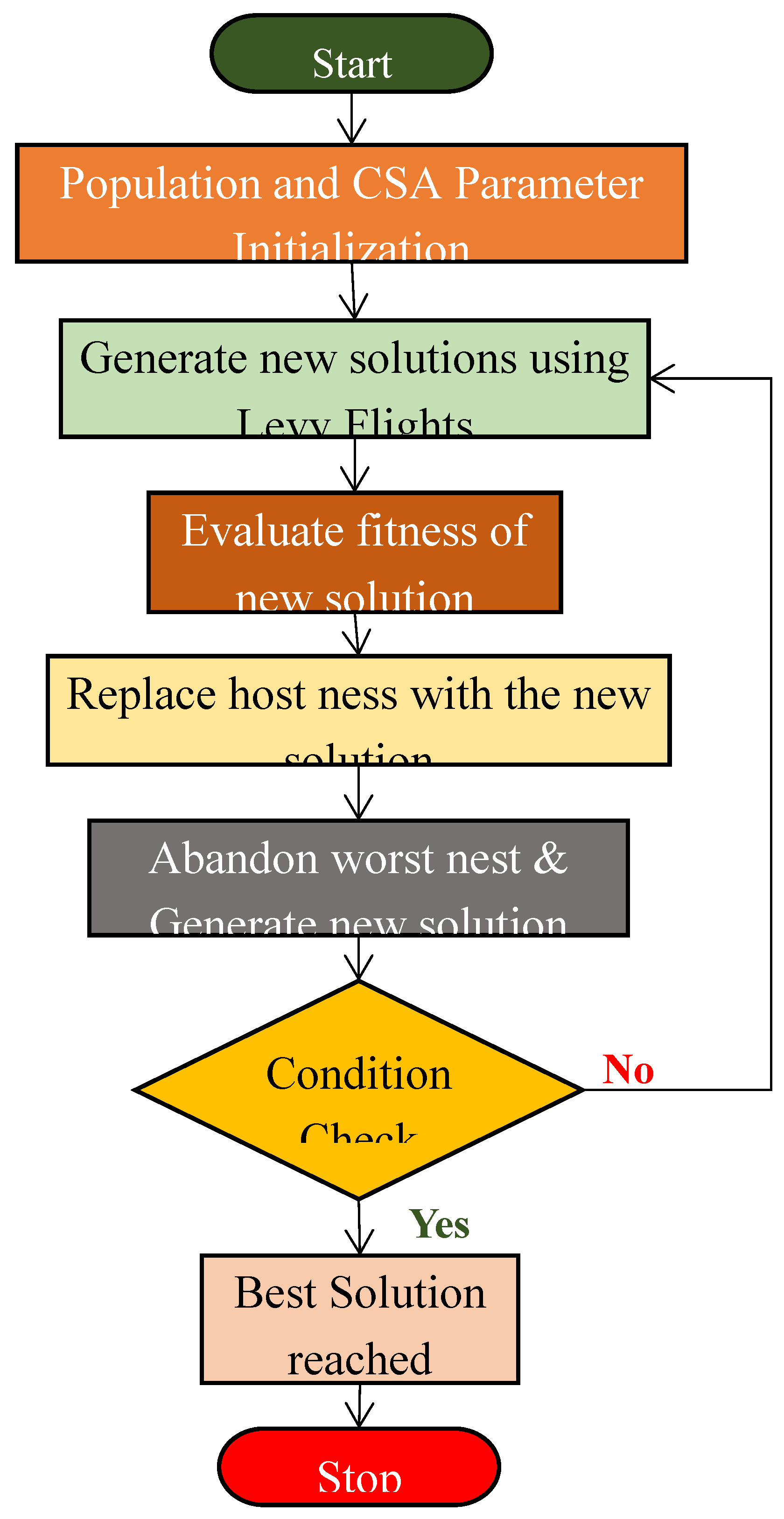
Figure 5.
Flow Chart representation of the Dragonfly Algorithm.
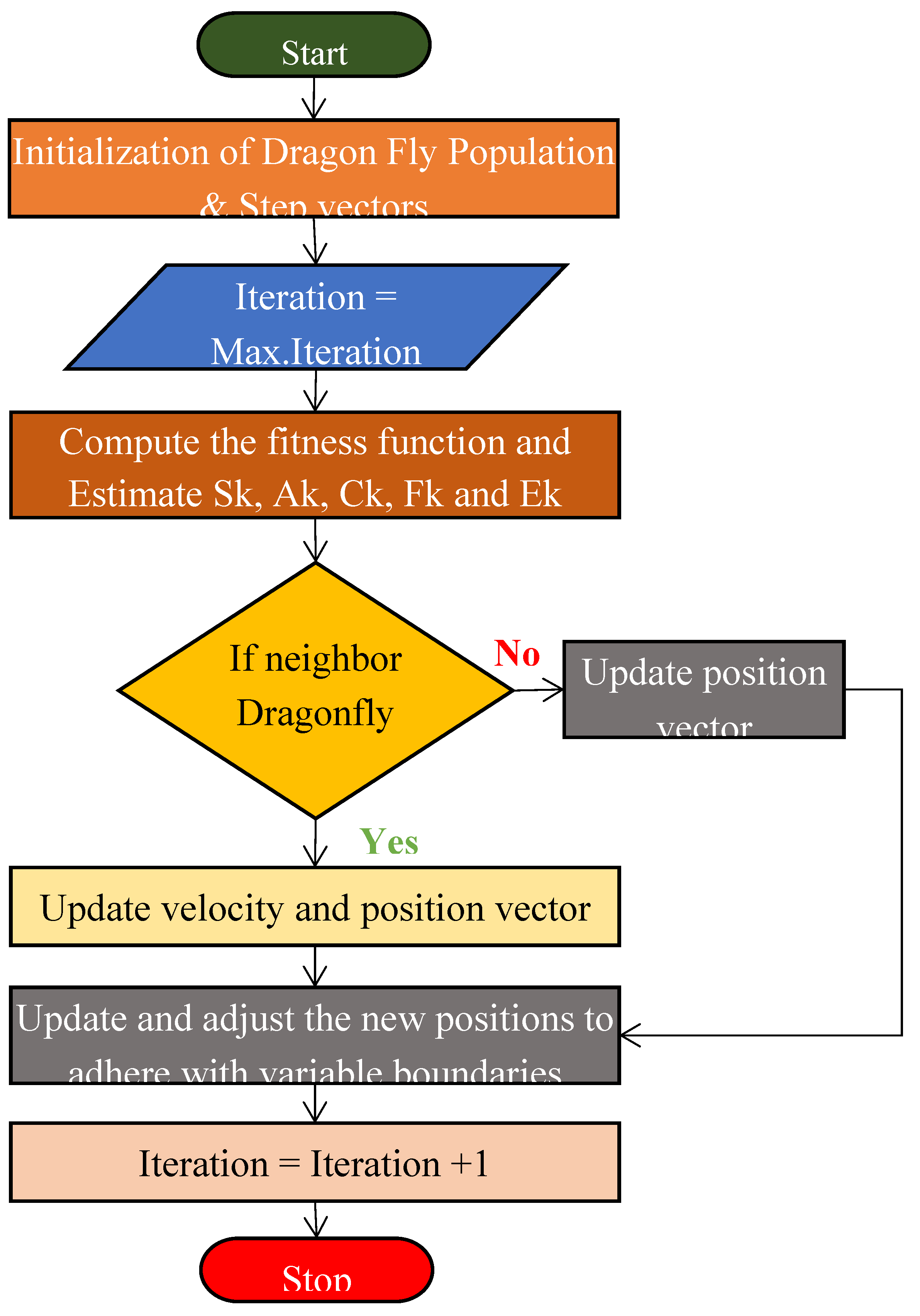
Figure 6.
Histogram of ABC PSO DR PPG signals for Normal Person.
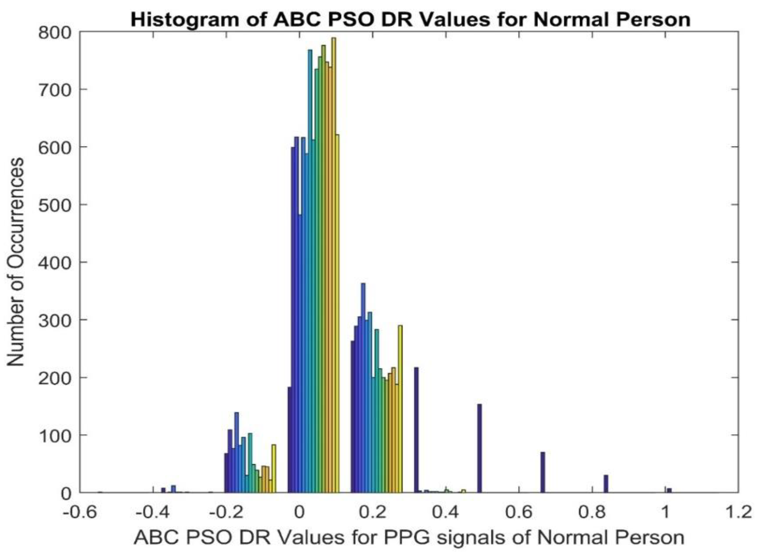
Figure 7.
Histogram of ABC PSO DR PPG signals for CVD Patient.
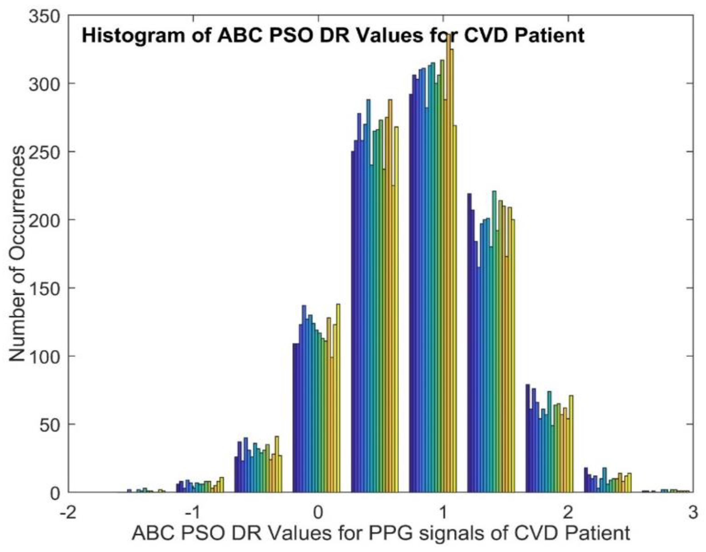
Figure 8.
Scatter Plot of ABC PSO based DR values of PPG signals.
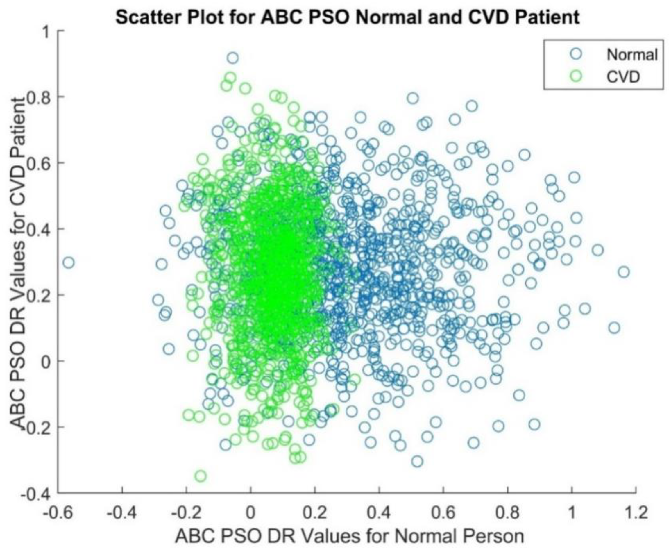
Figure 9.
Scatter Plot of Dragon Fly based DR values of PPG signals.
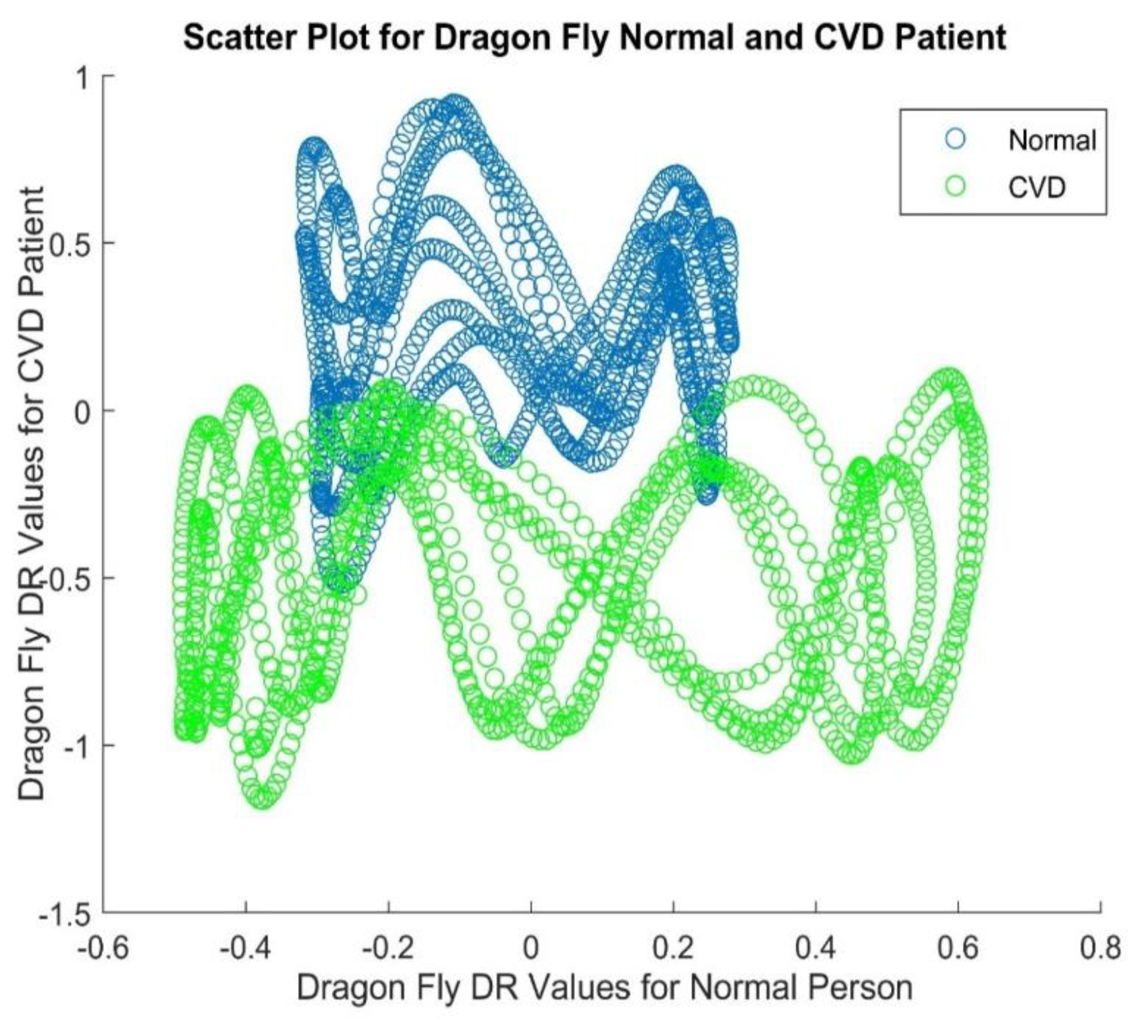
Figure 10.
Accuracy performance across various classifiers with DR Techniques.
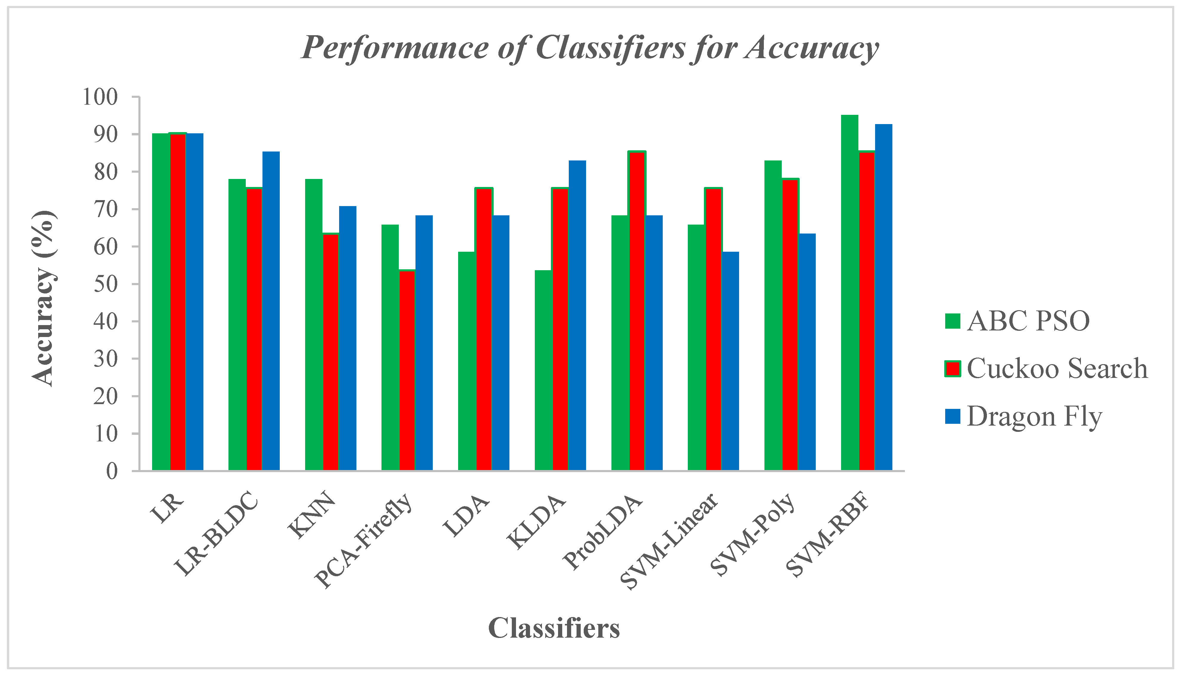
Figure 11.
Significance of Error Rate and F1 Score Performance of Classifiers for different DR Techniques .
Figure 11.
Significance of Error Rate and F1 Score Performance of Classifiers for different DR Techniques .
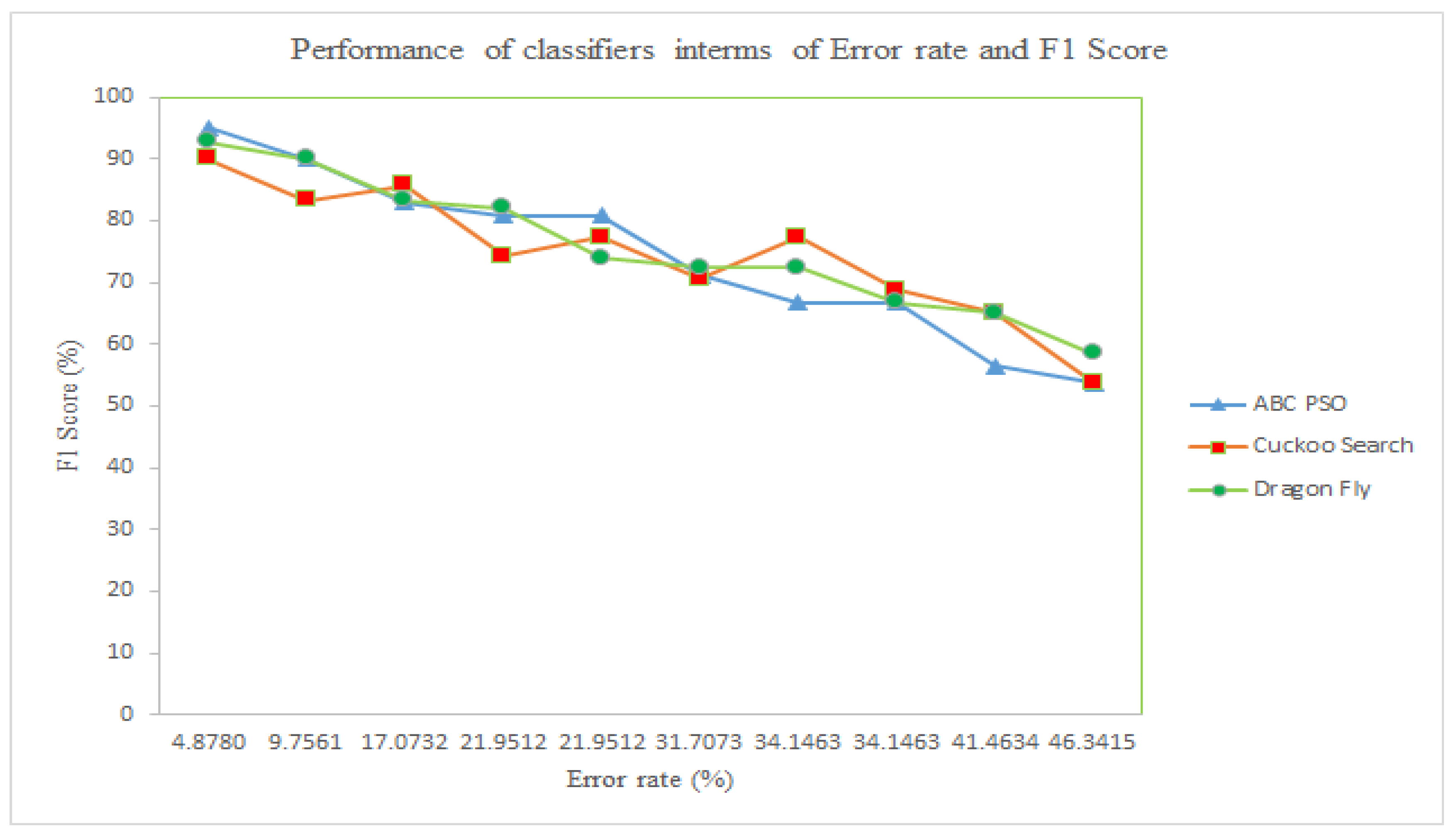
Figure 12.
Significance of Accuracy and Jaccard Index Performance of Classifiers.
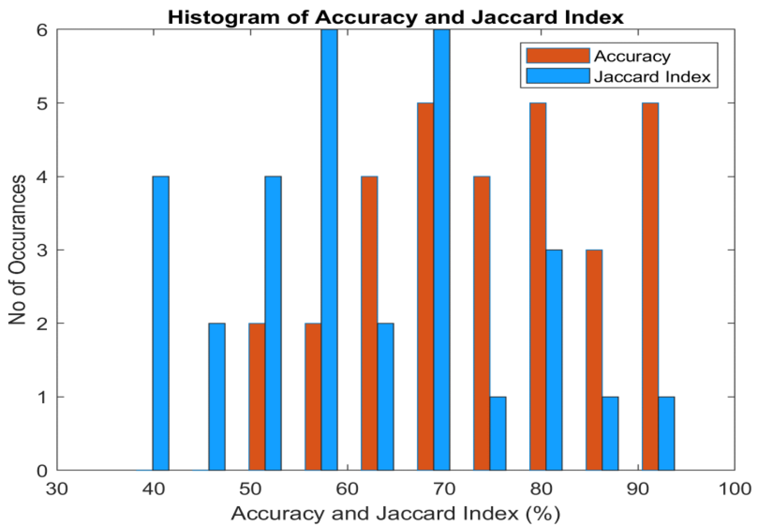

Table 1.
Selection of parameters for heuristic Algorithms.
| Parameters | Heuristic Algorithms | ||
| ABC-PSO | CSA | DFA | |
| Population Size | 200 | 200 | 200 |
| Control parameters | Inertia weight :0.45 Acceleration coefficients and |
Probability =0.4 Step Size α=1.5 |
Separation alignment cohesion Attraction Distraction |
| Algorithm | Swarm intelligence With Hybrid | Levy flight | Swarm intelligence |
| Stopping Criteria | Training MSE of 10-5 | Training MSE of 10-5 | Training MSE of 10-5 |
| Number of iteration | 200 | 200 | 200 |
| Local Minima Problem | Available in ABC. With proper selection of and in the PSO algorithm through trial and error method. The local minima problem will be solved. | No local minima problem | No local minima problem |
| Over fitting | Over fitting is available due to α and β values of ABC. This can be overcome with the proper selection of Weight (w) of PSO Algorithm | Over fitting is not presented | Over fitting is not presented |
Table 2.
Average Statistical Metrics of ABC-PSO, Cuckoo Search, and Dragonfly Dimensionality Reduction Methods for Normal and CVD Patients.
Table 2.
Average Statistical Metrics of ABC-PSO, Cuckoo Search, and Dragonfly Dimensionality Reduction Methods for Normal and CVD Patients.
|
Dimensionality Reduction Techniques |
Category | Statistical Metrics | ||||||
|---|---|---|---|---|---|---|---|---|
| Mean | Variance | Skewness | Kurtosis | PCC | Sample Entropy | CCA | ||
| Normal | 0.0732 | 0.0063 | -0.1165 | 0.2713 | -0.0597 | 9.9494 | 0.1066 | |
| CVD | 0.7872 | 0.3353 | -0.1000 | 0.1435 | 0.0133 | 9.9473 | ||
| Cuckoo search | Normal | 0.5236 | 0.0475 | 0.1575 | -0.4556 | 0.3393 | 9.9494 | 0.3674 |
| CVD | 7.8931 | 34.5391 | -0.0901 | -1.7290 | 0.2294 | 4.9919 | ||
| Dragon Fly | Normal | -1.5850 | 378.4756 | -0.0243 | -0.9585 | -0.2145 | 9.9499 | 0.4621 |
| CVD | -3.4728 | 271.9735 | 0.0381 | -0.6919 | 0.1044 | 9.9522 | ||
Table 3.
Comparative Analysis of Training and Testing Mean Square Error Across Various Dimensionality Reduction Approaches.
Table 3.
Comparative Analysis of Training and Testing Mean Square Error Across Various Dimensionality Reduction Approaches.
| Classifiers | ABC PSO | Cuckoo Search | Dragon fly | |||
|---|---|---|---|---|---|---|
| Training MSE | Testing MSE | Training MSE | Testing MSE | Training MSE | Testing MSE | |
| Linear Regression | 3.52E-09 | 2.92E-07 | 5.69E-09 | 1.37E-08 | 5.99E-09 | 1.44E-06 |
| Linear Regression with BDLC | 2.32E-06 | 1.10E-04 | 9.69E-08 | 8.65E-06 | 6.03E-08 | 2.72E-06 |
| KNN (weighted) | 5.72E-08 | 1.44E-06 | 4.60E-06 | 2.81E-03 | 7.02E-08 | 3.24E-06 |
| PCA firefly | 6.65E-07 | 3.80E-05 | 8.45E-06 | 6.08E-03 | 8.69E-06 | 6.25E-05 |
| LDA | 6.69E-05 | 5.48E-03 | 5.05E-06 | 1.44E-05 | 5.54E-06 | 2.70E-05 |
| KLDA | 7.34E-06 | 4.84E-03 | 4.63E-08 | 1.69E-06 | 6.63E-06 | 1.22E-05 |
| ProbLDA | 5.83E-06 | 3.06E-05 | 7.97E-08 | 6.76E-06 | 5.99E-07 | 1.68E-05 |
| SVM (Linear) | 4.05E-06 | 1.69E-04 | 4.85E-08 | 1.82E-06 | 7.89E-06 | 9.03E-03 |
| SVM (Polynomial) | 8.29E-08 | 6.76E-06 | 6.74E-08 | 1.44E-06 | 8.20E-07 | 7.29E-06 |
| SVM(RBF) | 1.92E-10 | 2.45E-09 | 5.38E-07 | 1.85E-05 | 2.45E-10 | 3.62E-09 |
Table 4.
Optimal Parameter Selection for Classifiers.
| Classifiers | Optimal Parameters of the Classifiers |
|---|---|
| Linear Regression (LR) | Uniform weight w=0.451, bias:0.003, Criterion: MSE |
| LR with BLDC | The cascading configuration of LR with the following BLDC parameters: Class mean and , Prior probability P(x): 0.5 |
| K-Nearest Neighbors (KNN) | Number of clusters = 2 |
| PCA Firefly |
PCA: A threshold value of 0.72 and decorrelated Eigen vector , using a trial and error training approach Firefly: Initial conditions of = 0.65, = 0.1 For both PCA and firefly, consider MSE of or reaching a maximum of 1000 iterations, whichever comes earliest. Criterion: MSE |
| Linear Discriminant Analysis (LDA) | Weight w=0.56,bias:0.0018 |
| Kernel LDA (KLDA) | Number of clusters:2, w1:0.38, w2:0.642, bias:0.0026±0.0001 |
| Probabilistic LDA(ProbLDA) | Weight w=0.56,bias:0.0018,Assigned Probability>0.5 |
| SVM-Linear | Class weights:0.4 Parameter for Regularization [C]:0.85 Criteria for Convergence : MSE |
| SVM-Polynomial | Parameter for Regularization [C]:0.76 Class weights:0.5 Kernel Function Coefficient [Gamma]:10 Criteria for Convergence : MSE |
| SVM-RBF | Parameter for Regularization [C]:1 Class weights:0.86 Kernel Function Coefficient [Gamma]:100 Criteria for Convergence : MSE |
Table 5.
Comparative Analysis of Classifiers on Dimensionality Reduced Features.
| DR Techniques |
Classifiers | Accuracy (%) |
GDR (%) | Error rate (%) | Kappa | MCC | F1 Score (%) |
JI (%) |
|---|---|---|---|---|---|---|---|---|
| ABC-PSO | Linear Regression | 90.24 | 89.74 | 9.76 | 0.80 | 0.80 | 90.00 | 81.82 |
| LR-BLDC | 78.05 | 72.73 | 21.95 | 0.56 | 0.60 | 80.85 | 67.86 | |
| K-Nearest Neighbors | 78.05 | 72.73 | 21.95 | 0.56 | 0.60 | 80.85 | 67.86 | |
| PCA Firefly | 65.85 | 57.58 | 34.15 | 0.32 | 0.32 | 66.67 | 50.00 | |
| Linear Discriminant Analysis | 58.54 | 48.48 | 41.46 | 0.17 | 0.17 | 56.41 | 39.29 | |
| Kernel LDA | 53.66 | 38.71 | 46.34 | 0.07 | 0.07 | 53.66 | 36.67 | |
| Probabilistic LDA | 68.29 | 59.38 | 31.71 | 0.37 | 0.38 | 71.11 | 55.17 | |
| SVM-Linear | 65.85 | 57.58 | 34.15 | 0.32 | 0.32 | 66.67 | 50.00 | |
| SVM-Polynomial | 82.93 | 81.08 | 17.07 | 0.66 | 0.66 | 82.93 | 70.83 | |
| SVM-RBF | 95.12 | 95.00 | 4.88 | 0.90 | 0.90 | 95.00 | 90.48 | |
| Cuckoo Search | Linear Regression | 90.24 | 89.74 | 9.76 | 0.80 | 0.80 | 90.00 | 81.82 |
| LR-BLDC | 75.61 | 70.59 | 24.39 | 0.51 | 0.52 | 77.27 | 62.96 | |
| K-Nearest Neighbors | 63.41 | 53.13 | 36.59 | 0.27 | 0.27 | 65.12 | 48.28 | |
| PCA Firefly | 53.66 | 38.71 | 46.34 | 0.07 | 0.07 | 53.66 | 36.67 | |
| Linear Discriminant Analysis | 75.61 | 74.36 | 24.39 | 0.51 | 0.53 | 70.59 | 54.55 | |
| Kernel LDA | 75.61 | 70.59 | 24.39 | 0.51 | 0.52 | 77.27 | 62.96 | |
| Probabilistic LDA | 85.37 | 85.00 | 14.63 | 0.71 | 0.72 | 83.33 | 71.43 | |
| SVM-Linear | 75.61 | 75.00 | 24.39 | 0.51 | 0.55 | 68.75 | 52.38 | |
| SVM-Polynomial | 78.05 | 76.92 | 21.95 | 0.56 | 0.58 | 74.29 | 59.09 | |
| SVM-RBF | 85.37 | 83.78 | 14.63 | 0.71 | 0.71 | 85.71 | 75.00 | |
| Dragon Fly | Linear Regression | 90.24 | 89.74 | 9.76 | 0.80 | 0.80 | 90.00 | 81.82 |
| LR-BLDC | 85.37 | 85.00 | 14.63 | 0.71 | 0.72 | 83.33 | 71.43 | |
| K-Nearest Neighbors | 70.73 | 62.50 | 29.27 | 0.42 | 0.44 | 73.91 | 58.62 | |
| PCA Firefly | 68.29 | 58.06 | 31.71 | 0.37 | 0.39 | 72.34 | 56.67 | |
| Linear Discriminant Analysis | 68.29 | 58.06 | 31.71 | 0.37 | 0.39 | 72.34 | 56.67 | |
| Kernel LDA | 82.93 | 81.58 | 17.07 | 0.66 | 0.66 | 82.05 | 69.57 | |
| Probabilistic LDA | 68.29 | 62.86 | 31.71 | 0.36 | 0.37 | 66.67 | 50.00 | |
| SVM-Linear | 58.54 | 46.88 | 41.46 | 0.17 | 0.17 | 58.54 | 41.38 | |
| SVM-Polynomial | 63.41 | 53.13 | 36.59 | 0.27 | 0.27 | 65.12 | 48.28 | |
| SVM-RBF | 92.68 | 92.50 | 7.32 | 0.85 | 0.85 | 92.68 | 86.36 |
Table 6.
Computational complexity for all classifiers across different DR methods.
| Classifiers | Heuristic dimensionality reduction techniques | ||
|---|---|---|---|
| ABC-PSO | CSA | DFA | |
| Linear Regression (LR) | |||
| LR with BLDC | |||
| K-Nearest Neighbors (KNN) | |||
| PCA Firefly | |||
| Linear Discriminant Analysis (LDA) | |||
| Kernel LDA (KLDA) | |||
| Probabilistic LDA(ProbLDA) | |||
| SVM-Linear | |||
| SVM-Polynomial | |||
| SVM-RBF | |||
Table 7.
Comparison of previous works on CVD classification using PPG signals.
| Sl.no | Authors | Dataset | Number of Subjects | Classifiers | Classes | Accuracy (%) |
|---|---|---|---|---|---|---|
| 1 | Rajaguru et al. [23] 2023 |
Capnobase dataset | Single patient | LR | CVD, Normal | 65.85% |
| 2 | Al Fahoum et al. [24] 2023 |
Internal medicine clinic of Princess Basma Hospital | 200 healthy and 160 with CVD | NB | Normal and abnormal | 89.37% |
| 3 | Prabhakar et al. [25] 2020 |
Capnobase dataset | 28 CVD 14 Normal |
SVM–RBF RBF NN |
CVD, Normal | 95.05% 94.79% |
| 4 | Liu et al. [27] 2022 |
GitHub https://github.com/zdzdliu/PPGArrhythmiaDetection |
45 Subjects | DCNN | CVD, Normal | 85% |
| 5 | Hosseini et al. [42] 2015 |
Tehran Heart Center | 18 Normal 30 CVD |
KNN | Low risk High risk |
81.5% |
| 6 | Miao and Miao [43] 2018 |
Cleveland Clinic Foundation | 303 patients | DNN | CVD, Normal | 83.67% |
| 7 | Shobita et al. [44] 2016 |
Biomedical Research Lab | 30 healthy 30 pathological | ELM | Healthy Risk of CVD |
89.33% |
| 8 | Soltane et al. [45] 2005 |
Seremban Hospital | 114 healthy 56 pathological | ANN | CVD, Normal | 94.70% |
| 9 | This research | Capnobase dataset | 21 Normal 20 CVD |
SVM-RBF | CVD, Normal | 95.12% |
LR-Linear regression; NB- Naive Bayes; DCNN-Deep Convolutional Neural Network; SVM-RBF- Support Vector Machine-Radial Basis Function; RBF NN-Radial Basis Function Neural Network; KNN- K-Nearest Neighbor; ELM- Extreme learning machine; DNN-Deep Neural Network; ANN-Artificial Neural Network;.
Disclaimer/Publisher’s Note: The statements, opinions and data contained in all publications are solely those of the individual author(s) and contributor(s) and not of MDPI and/or the editor(s). MDPI and/or the editor(s) disclaim responsibility for any injury to people or property resulting from any ideas, methods, instructions or products referred to in the content. |
© 2024 by the authors. Licensee MDPI, Basel, Switzerland. This article is an open access article distributed under the terms and conditions of the Creative Commons Attribution (CC BY) license (http://creativecommons.org/licenses/by/4.0/).
Copyright: This open access article is published under a Creative Commons CC BY 4.0 license, which permit the free download, distribution, and reuse, provided that the author and preprint are cited in any reuse.


