
Submitted:
06 July 2024
Posted:
08 July 2024
You are already at the latest version
Abstract
Environmental, social, and governance (ESG) investment has become a common trend in capital markets, and many institutional investors have publicly declared their long-term ESG investment target (ESGIT). This study focuses on investors who conduct strategic asset allocation (SAA) using composite indices but establish their ESGIT outside the SAA process. A mismatch could arise between investors’ planned and actual portfolios because they must pursue their ESGIT by asset selection, which inevitably makes the constituents of their portfolios different from those of composite indices. To scrutinize the potential existence of a misalignment between their SAA and ESGIT, this study analyzes actual stock and bond indices over the past decade using traditional mean-variance optimization. The results reveal significant differences between the expected and realized performances, and the misalignment is more significant when the analysis period is divided into two sub-periods: stable and volatile. Specifically, the results indicate that the efficient frontier constructed using ESG indices significantly differs from that constructed using composite indices, and that the difference between these two efficient frontiers becomes more significant during volatile periods. Furthermore, the results show that investors cannot meet their targets if their ESGIT is established outside the SAA process.
Keywords:
ESG Investment
; Sustainable Investment
; Strategic Asset Allocation
; ESG Investment Target
; Misalignment
1. Introduction
As sustainability has become an important issue globally, more investors have adopted environmental, social, and governance (ESG) investment. ESG investment is crucial for institutional investors such as pension funds, sovereign wealth funds, and insurance companies because their investment horizons are long, and investment performance is closely linked to overall economic growth. Government policies also drive institutional investors towards ESG investment. Thus, most governments have enacted regulations and incentives to promote ESG management of companies and real assets. Declaring a long-term ESG Investment target (ESGIT) is the first step in ESG integration, and institutional investors are no exception. Typical forms of ESGIT include the target year for achieving net-zero investments and the target proportion of sustainable assets in their portfolios. Since the Paris Agreement of 2015, most global investors have declared ESGIT. However, few investors have realistic plans for achieving their targets, which may lead to inefficient investment.
The investment processes of institutional investors are divided into two phases: asset allocation and asset selection. Strategic asset allocation (SAA), the long-term part of the asset allocation phase, determines the proportion of each asset class in the investment universe. Existing studies show that SAA plays a significant role in the overall investment performance. (Brinson et al. [1], Ibbotson and Kaplan [2]) However, the ESGIT and SAA of some institutional investors are established through separate processes. Many institutional investors establish their SAA based on quantitative methods, such as traditional mean-variance optimization (MVO), but determine their ESGIT through top-down approaches independent of their SAA processes. This practice is problematic, because it leads to inefficient investment performance. Most institutional investors establish their SAA using benchmark indices, such as composite indices, that reflect the average performance of each asset class. This supposes that in the subsequent asset selection phase, they aim to replicate the proportion of constituents of each composite index. However, when ESGIT is set separately and imposed in a top-down manner, investors must achieve the target during the asset selection phase. In other words, to increase the proportion of ESG investment, they must construct portfolios that differ from those suggested by their SAA.
This study analyzes the misalignment between SAA and ESGIT using actual stock and bond indices over the past decade. The analysis comprises two steps. First, portfolio optimization (SAA) is conducted using representative composite and ESG indices. Here, the efficient frontier derived from ESG indices is the result of integrating ESG factors into the SAA. Second, the performance of the optimized portfolio using composite indices (expected performance) is compared with realized performance that would be achieved by an investor. Realized performance is calculated by multiplying the weights of the constituents in the composite efficient frontier by the average returns of the ESG indices. This approach assumes that investors construct portfolios using the constituents of ESG indices during the asset selection process. These comparisons reveal the extent and pattern of misalignment between SAA and ESGIT, which is then applied to the entire decade and segmented periods before and after the COVID-19 outbreak to account for fundamentally different market conditions.
The remainder of this paper is organized as follows. Section 2 presents a literature review and specifies the unique features of this study. Section 3 introduces the materials and methods used in the study. Section 4 presents the portfolio optimization and performance analyses results. Lastly, Section 5 discusses the study’s findings and implications.
2. Literature Review
The most actively researched area concerning institutional investors’ ESG investment is the financial performance of sustainable portfolios. Considering that the greatest obstacle to adopting ESG investment is the concerns over investment return and risk, this can be seen as a natural phenomenon. Many studies have been conducted on ESG investment performance, and some address the performance of portfolios rather than individual assets.
Renneboog et al. [3] examine the investment performance and investor behavior of socially responsible investments (SRI). They compare the risk-adjusted returns of SRI funds with those of conventional funds and find that SRI funds perform well in some markets, but may underperform in some markets, such as those outside the US and the UK. Marlowe [4] uses financial econometrics to assess public pension funds’ involvement in SRI by leveraging data from thirteen large state government pension plans and finds significant SRI integration without compromising financial performance. Furthermore, he illustrates a shift in pension fund strategies towards incorporating ethical and social governance criteria. Becchetti et al. [5] evaluate the profitability of portfolios comprising socially responsible firms using advanced analytical techniques such as rolling window wavelets. They find that SRI funds exhibit low correlation with each other, suggesting that the funds provide beneficial diversification effects. Their findings support the inclusion of diverse SRI assets in portfolios to optimize returns and reduce risks. Rehman and Vo [6] scrutinize the profitability of investing in socially responsible firms by employing correlation and causality analyses across various SRI funds. They underscore that while SRI funds are generally profitable and offer substantial risk-adjusted returns, SRI funds’ performance relative to traditional funds vary. More importantly, they highlight SRI’s potential to attract more risk-averse investors, thereby broadening the appeal of ethical investments. Whelan et al. [7] conduct a comprehensive meta-analysis of the link between ESG factors and financial performance, aggregating over thousand studies from 2015 to 2020. They discover that most studies find a positive relationship between robust ESG practices and superior financial performance at both the corporate and investment levels, reinforcing the financial viability of responsible investing. Gomes [8] explores the dynamics of optimal growth under SRI using a theoretical model that encapsulates the tradeoffs between financial gains and emotional rewards. He introduces the ‘warm glow’ effect concept, in which investors derive satisfaction from ethically sound investments. His findings suggest that investors are willing to accept lower financial returns due to the perceived social and ethical benefits of their investments.
Unlike in the 1990s when opinions on the financial performance of ESG investment are sharply divided, most studies since the late 2000s argue that ESG investment performance is not inferior to that of traditional investment. This shift has led to advancements in the research on methodologies for sustainable SAA. Some studies have focused on SAA methodologies that consider ESG factors. Notably, studies, such as that of Gomes [6], focus not only on financial returns and risk but also on the utility derived from ethical values. In other words, they address techniques for quantitatively incorporating ESG factors into portfolio optimization.
Hallerbach et al. [9] introduce a method in which social responsibility attributes are measured and integrated into the asset allocation process. This framework uses a multi-attribute portfolio model to systematically compare portfolios based on ESG attributes, enabling dynamic interaction between investment manager preferences and portfolio outcomes. It allows customized portfolios to balance financial returns with social impacts. Jessen [10] extends the utility theory and mean-variance analysis by incorporating ESG preferences directly into investors’ utility functions. This integration allows for the adjustment of portfolio weights to reflect investors’ ESG preferences, ensuring that portfolios align with both financial and ethical objectives. Jin [11] explores the implications of ESG factors on US equity mutual funds by employing an enhanced five-factor model that incorporated an ESG factor. He reveals that ESG factors are systematically priced in the market, suggesting that responsible investing can be financially advantageous. Klement [12] focuses on the practical applications of ESG integration into asset allocation by employing a resampled efficient frontier optimizer to better handle estimation errors. He demonstrates how ESG factors can be incorporated into traditional portfolio optimization without significantly affecting the risk-return profile. Zerbib’s [13] sustainable capital asset pricing model (S-CAPM) modifies the traditional CAPM to include ESG factors. S-CAPM differentiates conventional from sustainable investors, illustrating how ESG integration affects asset pricing and provides a hedge against specific risks. Anatoly [14] incorporates ESG considerations into Dow Jones Index portfolios using an expanded mean-variance framework that introduces an ESG tilted Sharpe ratio, allowing for the optimization of portfolios that consider financial returns, risks, and ESG factors. Pedersen et al. [15] develop the concept of an ESG efficient frontier by adapting the traditional efficient frontier to include ESG scores as constraints. Their method facilitates the exploration of trade-offs between traditional financial returns and ESG performance, providing a robust framework for constructing portfolios that meet specific ESG criteria without sacrificing financial efficiency. Grim et al. [16] propose a framework that quantifies non-pecuniary utility from ESG features using investors’ willingness to pay for ESG compliance to adjust asset allocation in a portfolio. Their model balances financial objectives with ESG goals, allowing for highly customizable asset allocation.
The abovementioned methodologies highlight the trend toward more sophisticated asset allocation strategies that incorporate ESG criteria along with traditional financial metrics. These frameworks vary in complexity and application but collectively advance the integration of sustainability into financial decision-making. However, they are currently under development and most institutional investors still use traditional optimization techniques. Consequently, the risk mismatch between an actual investment portfolio and its strategic asset allocation becomes inevitable [17]. Unfortunately, existing studies that quantitatively test the existence of such mismatches are scarce. This study differs from previous studies as it quantitatively measures the possible loss of financial utility when an investor using traditional SAA sets and pursues ESGIT independently of SAA.
3. Materials and Methods
3.1. Analysis Data
This study utilizes widely used return indices for portfolio optimization because representative indices are relatively free from data selection bias. Aside from being well-known, the return indices should satisfy two additional requirements. First, the indices should have a long history, as the analysis period is 10 years. Second, the indices should be paired into the composite and ESG indices. In addition to the proportion of constituent assets, the other conditions between the two indices should be almost identical.
Table 1 lists the selected indices. We create a portfolio with four asset classes: stocks in advanced markets, stocks in emerging markets, treasury bonds in global markets, and corporate bonds in global markets. For stocks, Dow Jones and MSCI provide paired index sets with composite and ESG indices. For bonds, Bloomberg and MSCI provide ESG indices that correspond to the composite indices. Then, we conduct SAA with two data groups, Dow Jones–Bloomberg and MSCI–Bloomberg, and compare the performances of the composite and ESG efficient frontiers in each data group.
Figure 1 shows the stock market trends. According to the Dow Jones Indices, stock markets have been stable before the COVID-19 outbreak in 2020 but have become volatile after 2020. From 2020 to 2023, stock markets in developed markets have significantly increased, while those in emerging markets have struggled. The difference between the performance of the ESG and composite indices is greater in emerging markets. Figure 2 shows that the trends of the MSCI indices are similar.
Figure 3 shows the trends in bond markets. According to Bloomberg Indices, bond markets have also been stable before the COVID-19 outbreak in 2020; however, they have become extremely volatile immediately after 2020, similar to stock markets. From 2020 to 2023, the bond markets have faced difficult challenges such as interest rate hikes. Both treasury and corporate bond markets have significantly decreased during the period.
Figure 4 and Table 2 summarize the performances of all the selected indices. We find that stocks in developed markets have performed better than those in emerging markets, and that corporate bonds have performed better than treasury bonds over the last 10 years. Table 3 presents the correlations between these indices. Because of asset price synchronization in a volatile market, all correlations are positive.
3.2. Analysis Model
As described in Section 1, the analysis comprises two steps: portfolio optimization and a performance comparison between the expected and realized efficient frontiers. Both steps are applied to the entire 10 years and the segmented periods before and after the COVID-19 outbreak. Since MVO’s introduction in the 1950s, many quantitative models have been developed for portfolio optimization. To overcome the weakness of MVO, they employ multiple factors aside from market return, they use consumption or production beta rather than the wealth-based beta, and they analyze multiple or continuous periods instead of a single period. However, this study adopts the traditional MVO for two reasons. First, although practical advances have been made, no model has been perfect. In contrast, the MVO is straightforward and easy to understand. Second, this analysis does not aim to develop a better optimization model, but rather to compare the performance of portfolios constructed using composite and ESG indices. As suggested by Occam’s razor, applying the simplest model in such comparisons helps minimize the bias caused by unnecessary variables. This study applies no constraints other than full investment without short selling.
The performances are compared in three ways: First, we use standard deviation to measure risk. The range of risk investors can take is fundamental to performance. If this range is wide, investors can enjoy more portfolio choices. Second, we compare the returns of efficient frontiers for the same risk level. If an efficient frontier exhibits higher returns than another in the same risk range, we conclude that it performs better. Third, We conduct a t-test using returns within the same risk range to know the significance of the difference between returns.
4. Results
4.1. Whole Period: 2014~2023
4.1.1. Portfolio Optimization
To compare the risk-return characteristics of the portfolios constructed by composite and ESG indices, we conduct traditional MVO with the constraint of positive full investment of funds, which does not allow both short selling and idle money. The achievable return ranges are first calculated. Then, portfolios with minimum standard deviations are calculated for the 100 return levels between the minimum and maximum returns. Here, the minimum return is the return of the minimum variance portfolio, and the maximum return is the return of the portfolio that contains only one asset class with the highest return. We compare 20,000 portfolios for each return level.
Figure 5 presents the portfolio optimization results. Four types of efficient frontiers are presented. The portfolio optimization is divided into two groups by stock index provider: Dow Jones and MSCI. Then, each group is further divided into two sub-groups based on the characteristics of the composite and ESG indices. The upper panel shows the composite and ESG efficient frontiers constructed using the Dow Jones stock indices and Bloomberg bond indices. As revealed by the risk-return coordinate plane on the left, the two efficient frontiers have different risk-return characteristics. Broadly speaking, investors can achieve lower-risk asset allocation using ESG portfolios and higher-return asset allocation using composite portfolios. The risk-adjusted returns of the ESG portfolios are better in low-risk areas and those of the composite portfolios are better in high-risk areas. The weights of the asset classes are significantly different in low-risk areas, as shown in the bar charts on the right. The stocks in emerging markets are excluded. The weights of treasury and corporate bonds change dramatically in low-risk areas, and the weights of stocks in developed markets dominate high-risk areas. Practically, the portfolios in extremely high-risk areas are meaningless because the highest-risk portfolio is set as 100% developed market stocks.
The lower panel shows the composite and ESG efficient frontiers constructed using the MSCI stock indices and Bloomberg bond indices. Most results are similar to those in the upper panel, except that the risk-adjusted returns of the ESG portfolios are slightly better, even in high-risk areas. This might be because ESG stock indices and composite stock indices have similar performances in developed markets, as shown in the lower panel of Figure 2.
Table 4 shows that the risk range of the ESG efficient frontier is wider than that of the composite efficient frontier. The ESG efficient frontier expands far to lower-risk areas, while it is less risky in high-risk areas.
To compare the risk-adjusted financial performance of the two efficient frontiers, we select portfolios of the same risk range from the two efficient frontiers, which is the intersection of the two efficient frontiers in terms of risk level. Table 5 presents the return statistics. In Dow Jones efficient frontiers, the return of the ESG efficient frontier is higher than that of the composite efficient frontier in low-risk areas, and vice versa in high-risk areas. However, in MSCI efficient frontiers, the return of the ESG efficient frontier is higher than that of the composite efficient frontier in all risk areas. Table 6 presents the significance of these differences. The difference is significant in the MSCI indices at the 5% level but not in the Dow Jones indices.
4.1.2. Expected and Realized Performances
The main reason for the misalignment between institutional investors’ SAA and ESGIT is the current practice, in which the SAA is conducted with composite indices while establishing the ESGIT outside their SAA processes. The degree of misalignment can be measured using the difference between the expected and realized efficient frontiers. For the abovementioned investors, the expected efficient frontier is that of the composite indices, because they conduct optimization with those indices in the asset allocation stage. In contrast, their realized efficient frontier is the product of the weights of asset classes in the portfolios of the composite efficient frontier and the returns of the ESG indices because they select ESG stocks and bonds while allocating their funds according to SAA.
Realized performance may be better or worse than expected. During the last decade, it is similar to the ESG efficient frontier, as shown in Figure 6. Consequently, the misalignment is almost the same as the difference between the composite and ESG efficient frontiers reviewed above, indicating that the weights of the asset classes in the portfolios of the composite and ESG efficient frontiers are not significantly different across all risk areas.
Table 7 shows that the realized risk range is wider than the expected risk range. The realized efficient frontier expands far into lower-risk areas, whereas it is less risky in high-risk areas. This result implies that investors achieve lower risks and returns than expected if they pursue sustainability during the asset selection phase.
Table 8 shows the return statistics for intersection risk levels. In the Dow Jones efficient frontiers, realized returns are higher than the expected returns in low-risk areas, and vice versa in high-risk areas. However, in the MSCI efficient frontiers, realized returns are higher than expected returns in all risk areas. Table 6 presents the significance of these differences. The misalignment is significant in the MSCI indices at the 5% level but not in the Dow Jones indices. Although the misalignment is not consistent among the index providers, we conclude that it is not negligible.
The results meet the general expectations. Over the last decade, ESG portfolios have provided better results for risk-averse investors. However, the COVID-19 outbreak could have affected these results. A deeper understanding of the difference between the composite and ESG portfolios may be captured by conducting the same analysis during stable and volatile periods.
4.2. Before the COVID-19 Outbreak: 2014~2019
4.2.1. Portfolio Optimization
The financial performance of all asset classes is stable before the COVID-19 outbreak. Therefore, we can define this period as normal in contrast to the later period. Table 10 presents the statistics of selected indices during this period.
Figure 7 shows that the results of the traditional MVO significantly differ from those of the entire period. In the upper panel, the Dow Jones stock indices and the Bloomberg bond indices show that the ESG efficient frontier has a broader risk range in both low- and high-risk areas (Table 11), and the composite efficient frontier achieves higher returns at all intersection risk levels. The composite portfolios are constructed using only two asset classes, stocks in the developed market and corporate bonds, whereas the ESG portfolios also include treasury bonds. In the lower panel, MSCI stock indices and Bloomberg bond indices show different patterns from the others. The ESG efficient frontier achieves a lower return in low-risk areas, and vice versa in high-risk areas. One distinct result is the weights of the asset classes. Stocks in emerging markets dominate asset allocations in high-risk areas, indicating that the financial performance of this asset class before the COVID-19 outbreak is significantly better than that after the outbreak.
Table 12 presents the return statistics for the intersection risk ranges. In the Dow Jones and Bloomberg efficient frontiers, the composite portfolios achieve higher returns in all risk levels. However, in the MSCI and Bloomberg efficient frontiers, the composite portfolios perform better in low-risk areas, and vice versa in high-risk areas. Table 13 shows that the difference between Dow Jones and Bloomberg efficient frontiers is significant but that between the MSCI and Bloomberg efficient frontiers is insignificant.
4.2.2. Expected and Realized Performances
Figure 8 and Table 14 presents the difference between expected and realized efficient frontiers. Despite the difference in return gaps, the two index sets exhibit the same pattern. The realized efficient frontiers perform worse than expected. This result may be due to the low risk-adjusted performance of the ESG investment under normal market conditions.
4.3. After the COVID-19 Outbreak: 2020~2023
4.3.1. Portfolio Optimization
The period between 2020 and 2023 is considered volatile. ESG or sustainable assets are expected to perform better than others under such conditions because they normally have a strong defense against ESG issues, and the empirical analysis using portfolio optimization confirms the assumption. Table 17 presents the statistics of selected indices during this period.
Figure 9 and Table 18 present the results of the portfolio optimization during the volatile period using the data in Table 17. ESG efficient frontiers are higher than composite efficient frontiers for all risk levels in the two index sets, and the weights of the asset classes are similar to those of the entire period. This indicates that asset allocations for the entire period are mainly affected by the volatility in this period.
In contrast to the results for the entire period, the difference between the composite and ESG efficient frontiers are significant. The results presented in Table 19 and Table 20 indicate that the difference is significant at the 1% and 5% levels for the Dow Jones and Bloomberg efficient frontiers and the MSCI and Bloomberg efficient frontiers, respectively.
4.3.2. Expected and Realized Performances
Similar to the results for the entire period, the differences between the expected and realized performances are comparable to those between the composite and ESG efficient frontiers. Figure 10 and Table 21 illustrates that the realized performances for the two index sets are better than expected, indicating that ESG or sustainable assets perform better than others in terms of risk-adjusted returns during turbulent conditions.
Table 22 and Table 23 present the results for the returns of expected and realized efficient frontiers after the COVID-19 outbreak. The difference between the expected and realized efficient frontiers during this volatile period is slightly less significant than that between the composite and ESG efficient frontiers. The difference is significant at the 5% and 10% levels for the Dow Jones and Bloomberg efficient frontiers and the MSCI and Bloomberg efficient frontiers, respectively. Thus, investors who adopted ESG investments during this period may have achieved better performance than expected.
4.4. Results Summary
This study makes two comparisons. First, this study compares efficient frontiers using composite and ESG indices. Specifically, it focuses on the difference between composite and ESG portfolios. The comparison shows the extent to which the SAA may differ according to the choice of indices. Second, this study compares the performance of expected and realized efficient frontiers. This comparison reveals the misalignment between the SAA and ESGIT of investors who conduct the SAA with composite indices and set the ESGIT outside of their SAA processes. The two comparisons are applied to three periods: the last ten years, stable period (2014-2019), and volatile period (2020-2023). Table 24 presents the results for these three periods.
During the entire period, ESG portfolios are less risky than composite portfolios. For Dow Jones and Bloomberg indices, the ESG portfolio returns are higher than composite portfolio returns in low-risk areas and vice versa in high-risk areas. For the MSCI and Bloomberg indices, ESG portfolio returns are higher than composite portfolio returns in all risk areas. Similar patterns are observed between expected and realized portfolios. However, the significance of these differences remains unclear. The differences is insignificant in the Dow Jones and Bloomberg efficient frontiers but significant at the 5% level in the MSCI and Bloomberg efficient frontiers.
During the stable period (2014-2019), the ESG portfolios show a wider risk range than the composite portfolios. In particular, the risk of ESG portfolios using the MSCI and Bloomberg indices is much higher than that of the composite portfolios. The returns also show different patterns according to the index set. In the Dow Jones and Bloomberg efficient frontiers, the ESG portfolios achieve much lower returns than the composite portfolios. In MSCI and Bloomberg efficient frontiers, the ESG portfolios achieve lower returns than the composite portfolios in low-risk areas, and vice versa in the higher-risk area in the MSCI and Bloomberg efficient frontiers. A similar pattern is observed between the expected and realized portfolios, except that the risk ranges of the realized portfolios are similar to that of the expected portfolios, and the returns of the realized portfolios are slightly lower than that of the expected portfolios in the MSCI and Bloomberg efficient frontiers. Overall, these differences are statistically significant.
During the volatile period (2020-2023), ESG portfolios perform better than composite portfolios. Their risk ranges are similar to those of the composite portfolios, and their returns are higher than those of the composite portfolios in the two index sets. A similar pattern is observed between the expected and realized portfolios. The difference is significant, indicating that ESG investment addresses market turbulence better than composite investment. Despite the better performance of ESG investment, this difference is also proves the existence of misalignment between the SAA and ESGIT.
5. Discussion
Pursuing sustainability has become a common trend for institutional investors such as pension funds, sovereign wealth funds, and insurance companies. Thus, professional services that support ESG investment such as ESG indices, ESG ratings, and ESG reporting have been developed. However, most developments have focused on asset selection during the investment process. Consequently, institutional investors may be exposed to inefficient SAA. This study focuses on institutional investors who conduct SAA using composite indices of asset classes but establish their ESGIT outside of the SAA process. This could lead to a mismatch between the portfolios that are planned in the SAA and those actually possessed because investors must pursue their ESGIT through asset selection, which makes the constituents of their portfolio different from those of composite indices. To scrutinize the misalignment between the SAA and ESGIT, this study analyzes actual stock and bond indices over the past decade. We conduct portfolio optimization using representative composite and ESG indices. Then, we compare the performance of the optimized portfolio or expected performance with realized performance using a top-down ESGIT. The results indicate a significant misalignment. The misalignment is more significant when the analysis period is divided into the stable period and volatile period.
Specifically, this study has three main findings. First, the results indicate that ESG investment has different risk-return characteristics from composite or ordinary investment. Therefore, the efficient frontier constructed using the ESG indices also differs from that constructed using the composite indices. Second, the results show that the difference between the two efficient frontiers becomes more significant during volatile periods. In particular, ESG portfolios provide better risk-adjusted returns than do composite portfolios. Third, the study suggests that investors cannot meet their financial targets if their ESGIT are established outside the SAA process. Regardless of the comparative advantage of ESG investment, a misalignment can cause inefficiencies in portfolio management. Therefore, investors should develop a methodology for integrating the SAA and ESGIT processes.
This study has several limitations. First, this study uses representative return indices. However, only pairs consisting of ESG and composite indices are selected. To generalize the results of this study, future analyses should use diverse sets of indices. Second, this study adopts the traditional MVO to control for possible bias caused by multiple variables. However, other optimization methods have advantages and can also control for bias. Therefore, to make the study’s results robust, future analyses must adopt other advanced models.
Conflicts of Interest
The authors declare that this study received funding from Mastern Investment Management Co. Ltd. The funder was not involved in the study design, collection, analysis, interpretation of data, the writing of this article or the decision to submit it for publication.
References
- Brinson, G.P.; Hood, L.R.; Beebower, G.L. Determinants of Portfolio Performance, Financial Analysts J. 1986, 42, 4.
- Ibbotson, R.G.; Kaplan, P.D. Does Asset Allocation Policy Explain 40, 90, or 100 Percent of Performance, Financial Analysts J. 2000, .56, 1.
- Renneboog, L.; Ter Horst, J.; Zhang, C. Socially responsible investments: Institutional aspects, performance, and investor behavior. J. Banking Fin. 2008, 32, 1723–1742. [CrossRef]
- Marlowe, J. Socially responsible investing and public pension fund performance. Public Perform. Manag. Rev. 2014, 38, 337–358. [CrossRef]
- Becchetti, L.; Ciciretti, R.; Dalò, A.; Herzel, S. Socially responsible and conventional investment funds: Performance comparison and the global financial crisis. Appl. Econ. 2015, 47, 2541–2562. [CrossRef]
- Rehman, M.U.; Vo, X.V. Is a portfolio of socially responsible firms profitable for investors? J. Sustain. Fin. Invest. 2020, 10, 191–212. [CrossRef]
- Whelan, T.; Atz, U.; Van Holt, T.; Clark, C. ESG and financial performance. Uncovering Relat. Aggregating Evid. from 2021, 1, 2015–2020.
- Gomes, O. Optimal growth under socially responsible investment: A dynamic theoretical model of the trade-off between financial gains and emotional rewards. Int. J. Corp. Soc. Respons. 2020, 5, 5. [CrossRef]
- Hallerbach, W.; Ning, H.; Soppe, A.; Spronk, J. A framework for managing a portfolio of socially responsible investments. Eur. J. Oper. Res. 2004, 153, 517–529. [CrossRef]
- Jessen, P. Optimal responsible investment. Appl. Financ. Econ. 2012, 22, 1827–1840. [CrossRef]
- Jin, I. Is ESG a systematic risk factor for US equity mutual funds? J. Sustain. Fin. Invest. 2018, 8, 72–93. [CrossRef]
- Klement, J. Does ESG matter for asset allocation? SSRN Journal 2018, Available at SSRN 3213134. [CrossRef]
- Zerbib, O.D. A Sustainable Capital Asset Pricing Model (S-CAPM): Evidence from green investing and sin stock exclusion (Working Paper). SSRN Journal 2020. [CrossRef]
- Anatoly, B.S. Optimal ESG portfolios: an example for the Dow Jones Index, J. Sustainable Finance & Investment, 2020. [CrossRef]
- Pedersen, L.H.; Fitzgibbons, S.; Pomorski, L. Responsible investing: The ESG-efficient frontier. J. Financ. Econ. 2021, 142, 572–597. [CrossRef]
- Grim, D.M.; Renzi-Ricci, G.; Madamba, A. Asset allocation with nonpecuniary ESG preferences: Efficiently blending value with values. In J. Invest. Manag. 2022.
- Lagerweij, Z.A. Detecting a Risk Mismatch Between Actual Investment Portfolio and Its Strategic Asset Allocation, 2012.
- Schmidt, A.B. Optimal ESG portfolios: An example for the Dow Jones Index. J. Sustain. Fin. Invest. 2022, 12, 529–535. [CrossRef]
Figure 1.
Dow Jones Stock Indices.
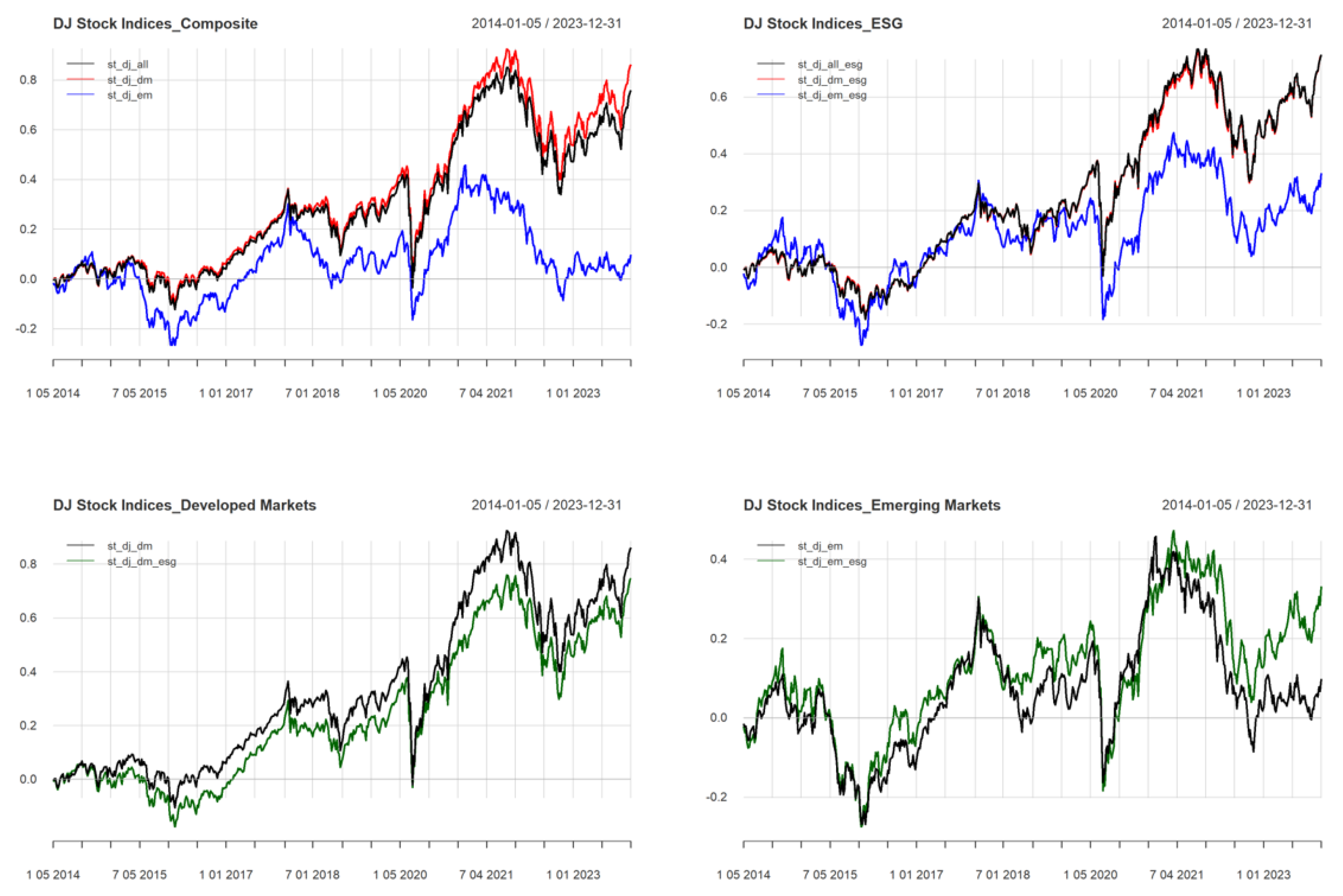
Figure 2.
MSCI Stock Indices.
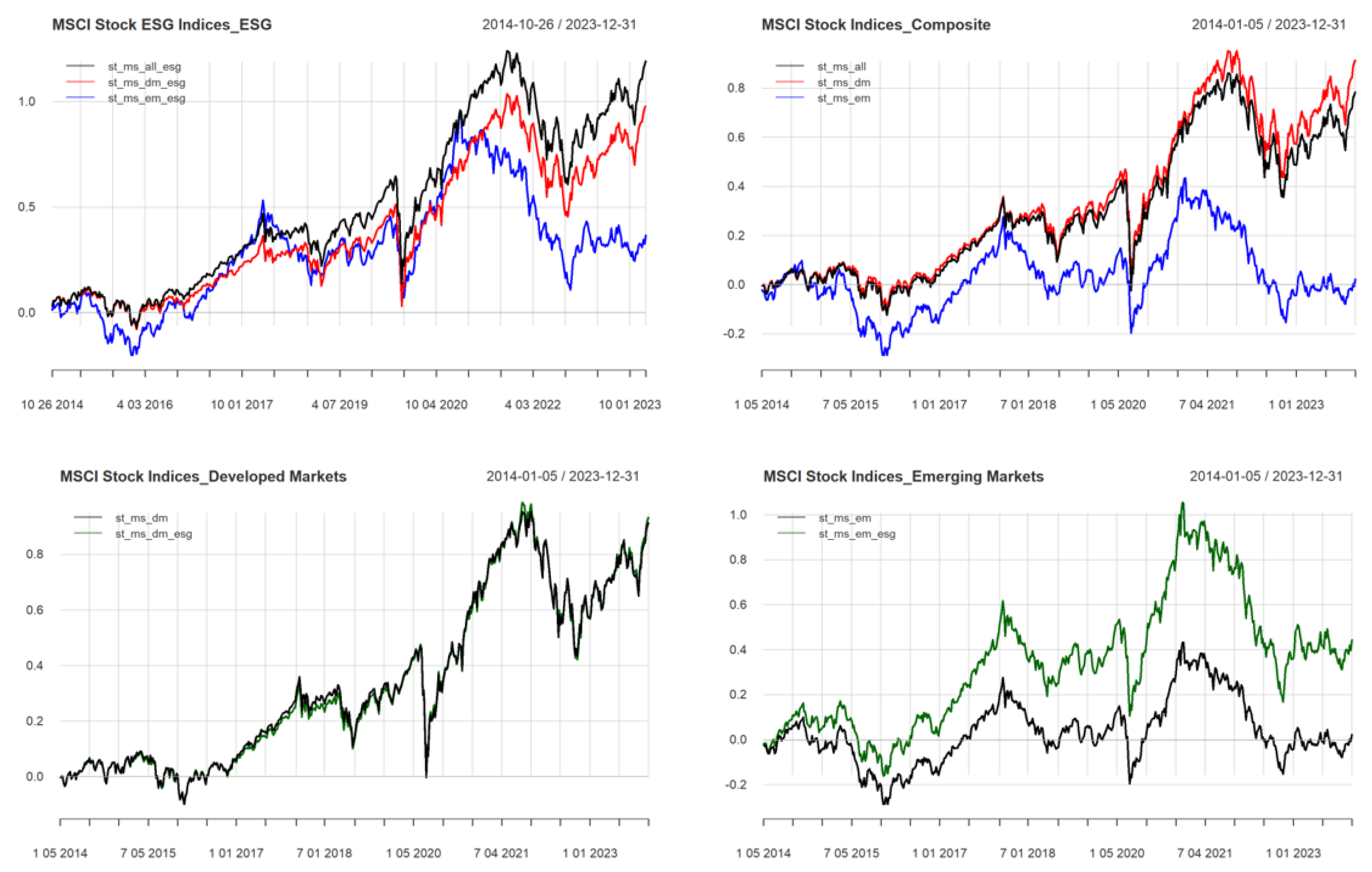
Figure 3.
Bloomberg Bond Indices.
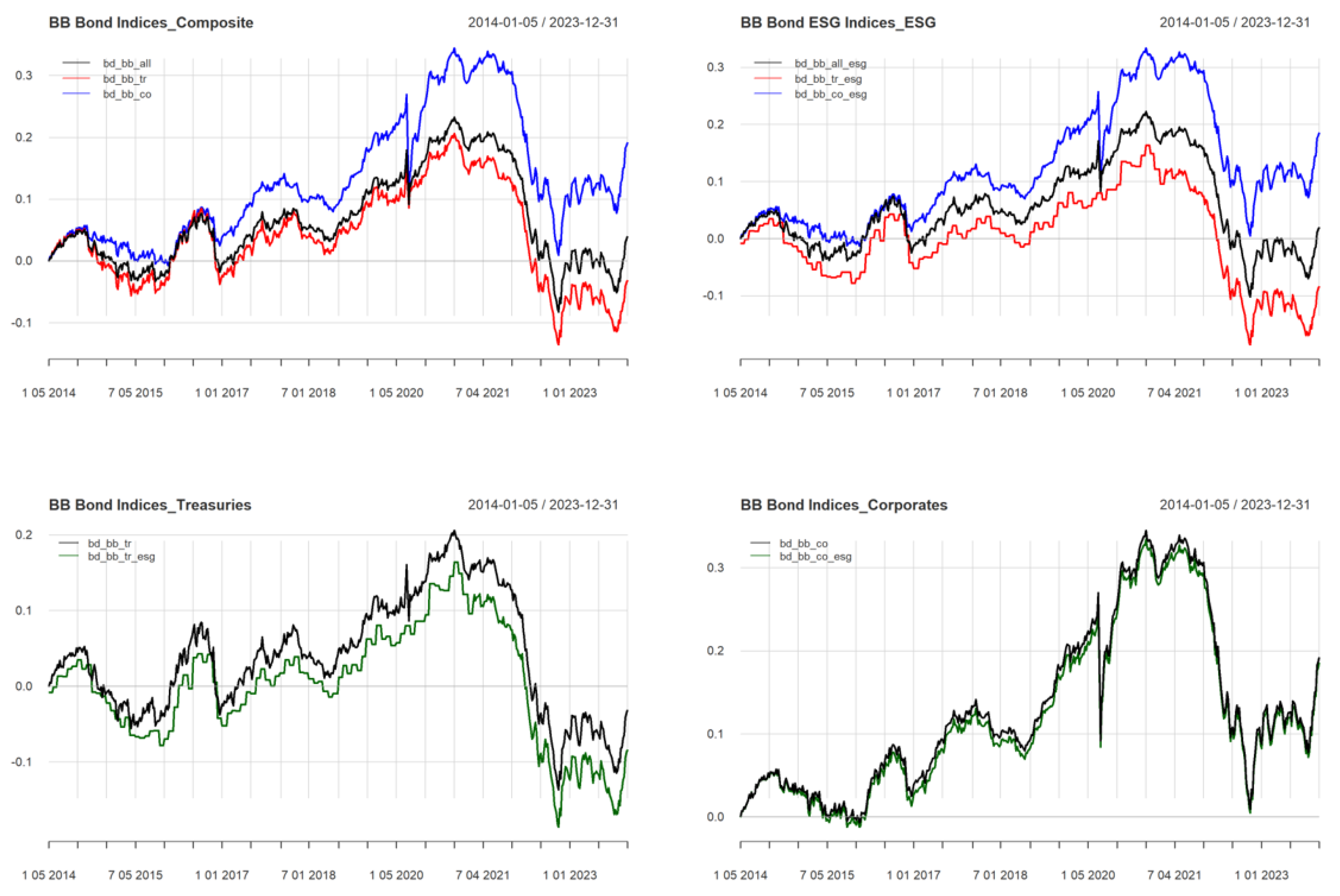
Figure 4.
Risk-Return of Selected Indices.
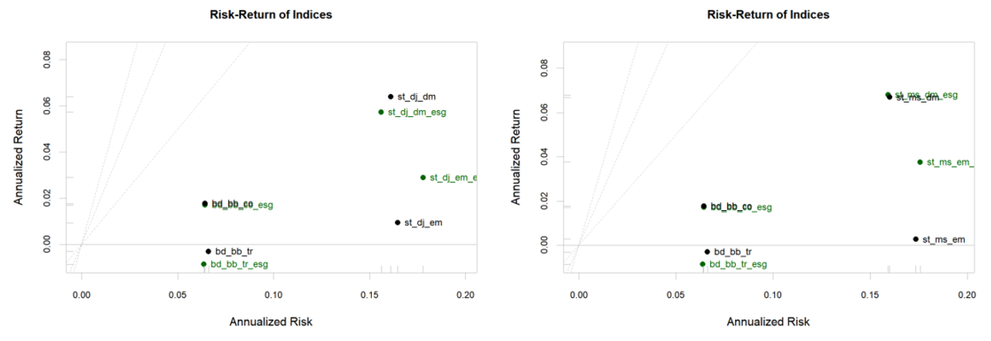
Figure 5.
Portfolio Optimization of the Whole Period.
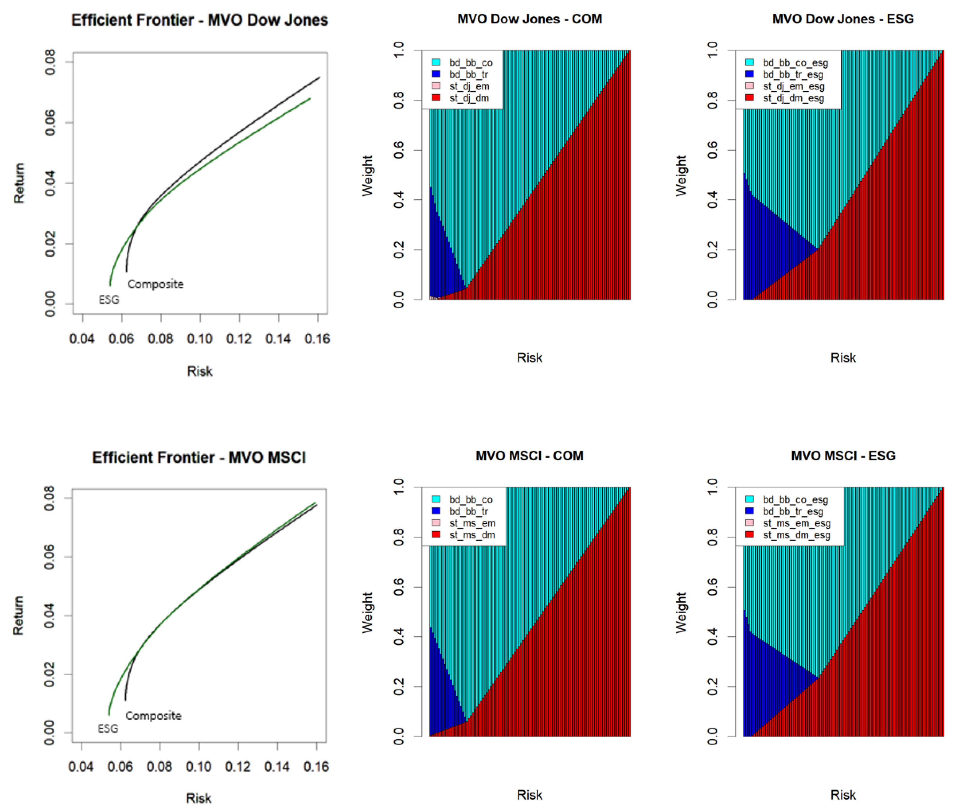
Figure 6.
Comparison of Expected and Realized Performances.
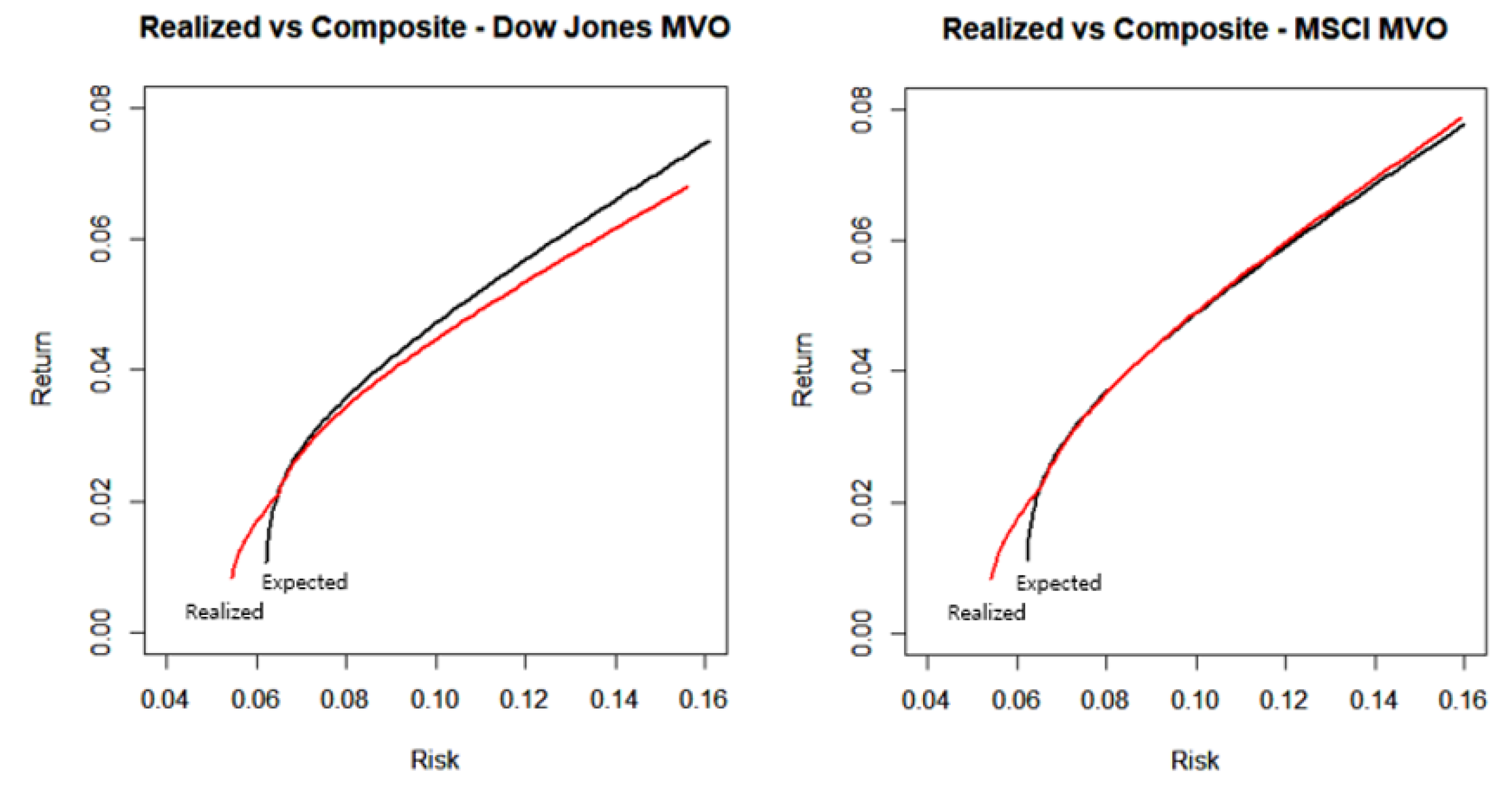
Figure 7.
Portfolio Optimization before the COVID-19 Outbreak.
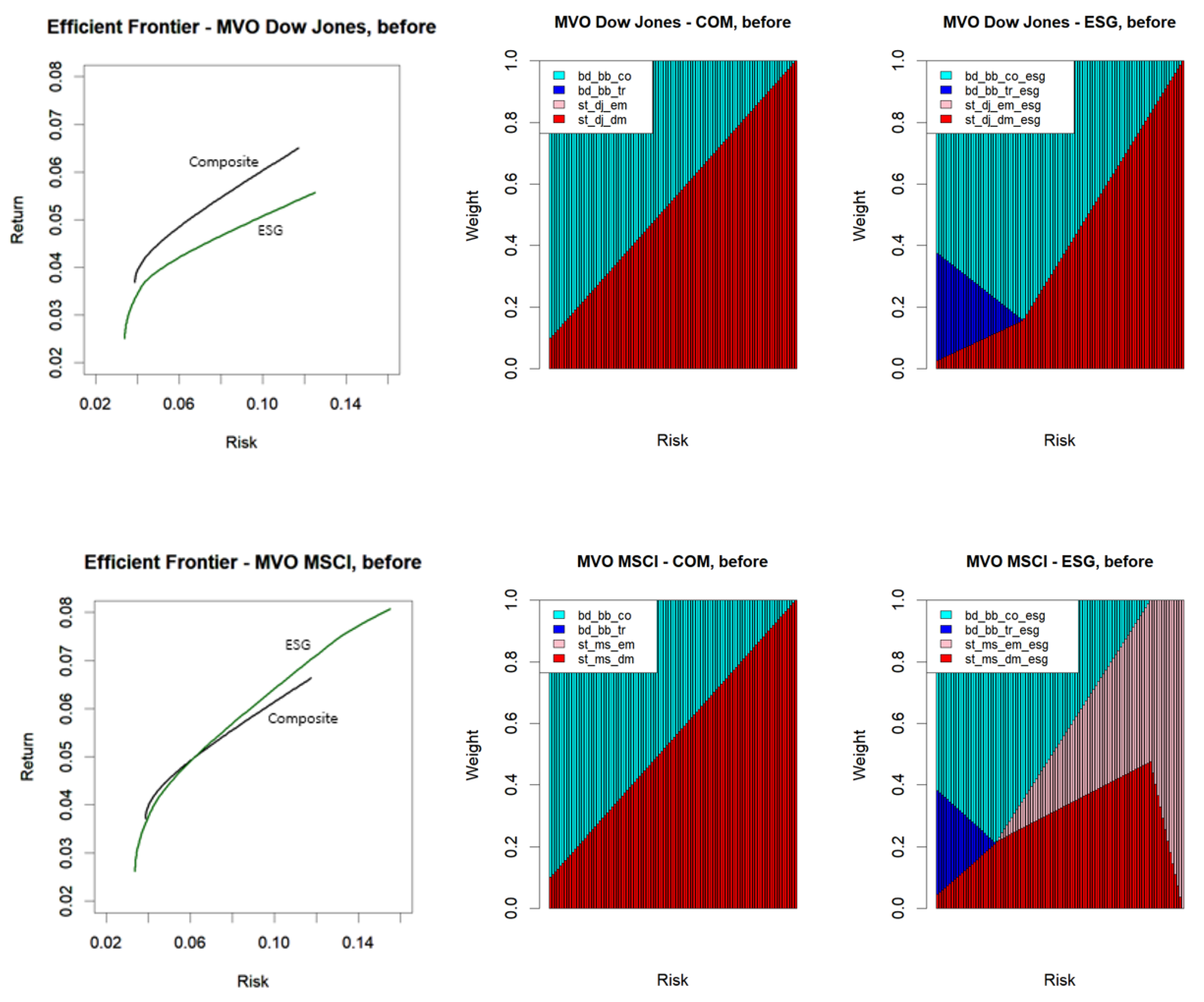
Figure 8.
Comparison of Expected and Realized Performance before the COVID-19 Outbreak.
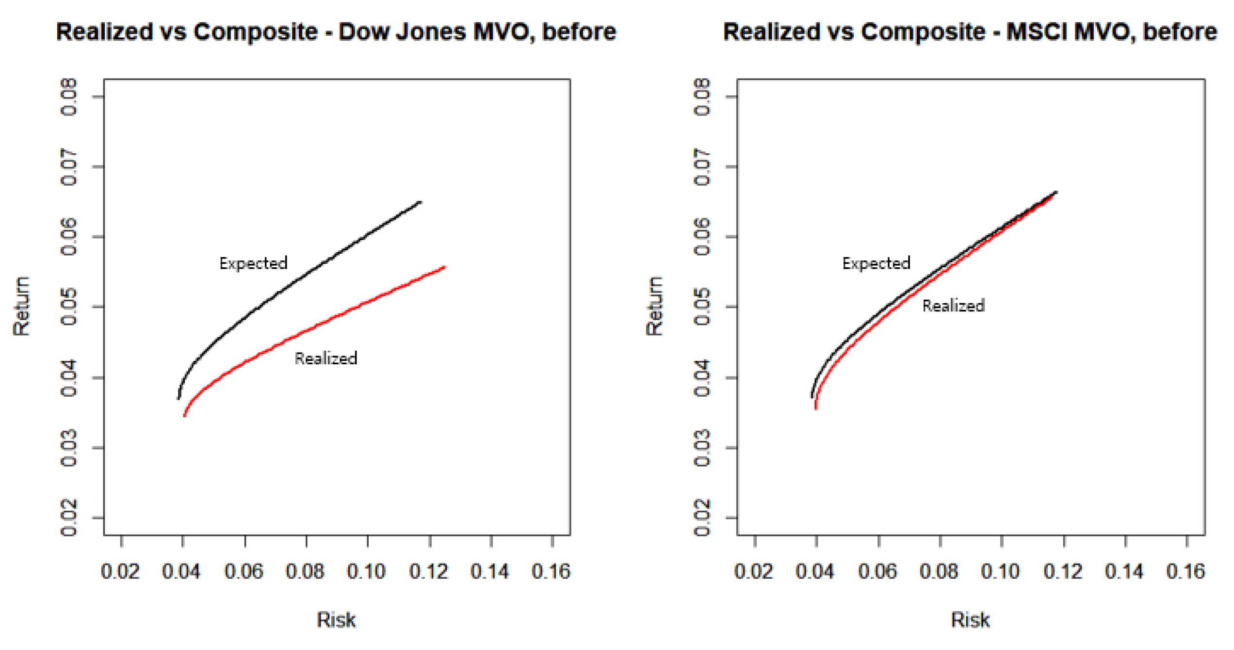
Figure 9.
Portfolio Optimization – Composite and ESG after the COVID-19 Outbreak.
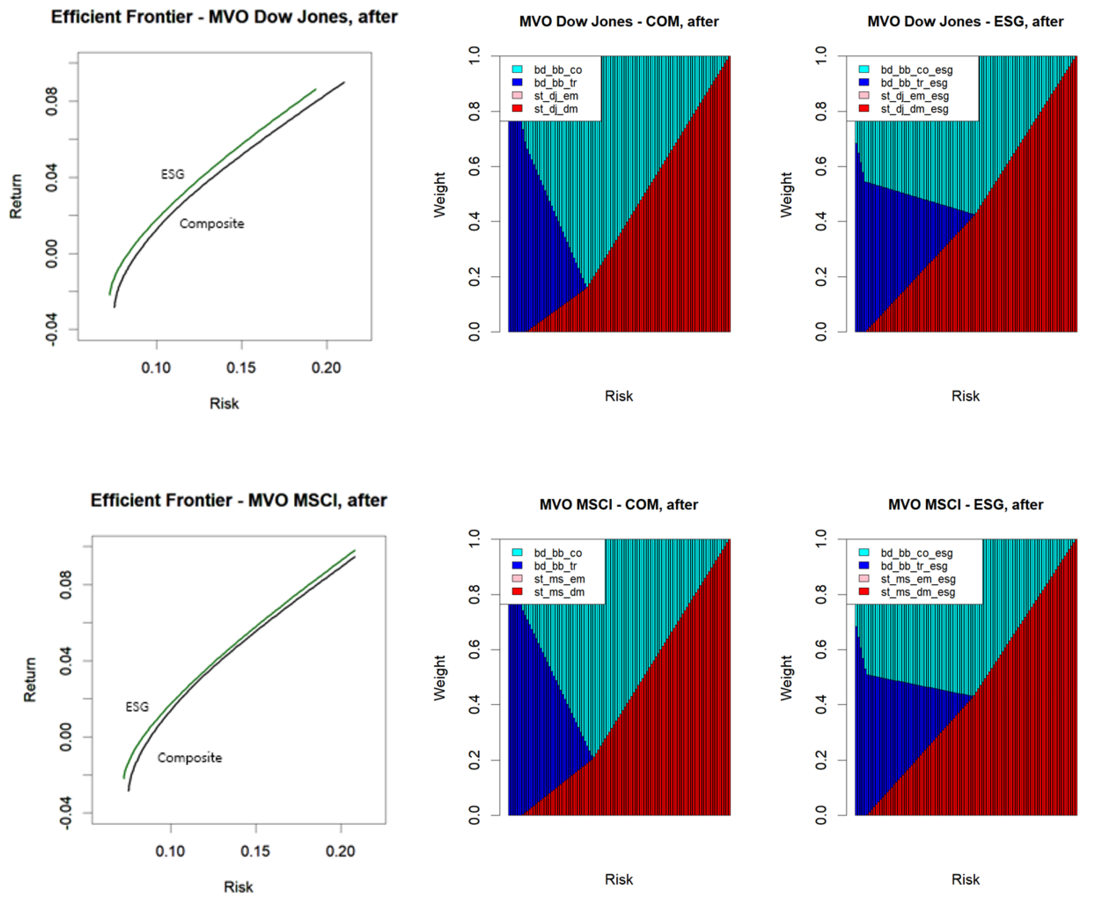
Figure 10.
Comparison of Expected and Realized Performances after the COVID-19 Outbreak.
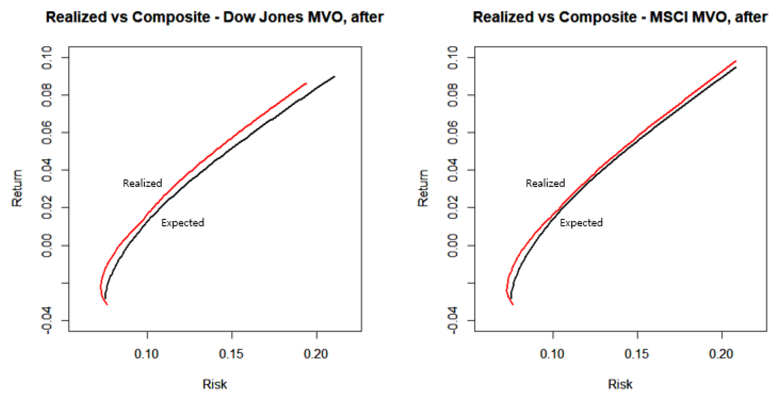

Table 1.
Selected Indices.
| Sector | Category | Name | Notation |
|---|---|---|---|
| Stock | Composite | Dow Jones Developed Markets | st_dj_dm |
| Dow Jones Emerging Markets | st_dj_em | ||
| ESG | Dow Jones Sustainability Developed Markets | st_dj_dm_esg | |
| Dow Jones Sustainability Emerging Markets | st_dj_em_esg | ||
| Composite | MSCI World | st_ms_dm | |
| MSCI Emerging Markets | st_ms_em | ||
| ESG | MSCI World ESG Leaders | st_ms_dm_esg | |
| MSCI Emerging Markets ESG Leaders | st_ms_em_esg | ||
| Bond | Composite | Bloomberg Global-Aggregate Treasuries TR | bd_bb_tr |
| Bloomberg Global Aggregate Corporate TR | bd_bb_co | ||
| ESG | Bloomberg MSCI Global Treasury ESG | bd_bb_tr_esg | |
| Bloomberg MSCI Global Corporate ESG | bd_bb_co_esg |
Table 2.
Statistics of Selected Indices.
| Min | Mean | Median | Max | SD | |
|---|---|---|---|---|---|
| st_dj_dm | -0.1292 | 0.0014 | 0.0023 | 0.1117 | 0.0223 |
| st_dj_dm_esg | -0.1254 | 0.0013 | 0.0024 | 0.0973 | 0.0216 |
| st_dj_em | -0.1156 | 0.0004 | 0.0023 | 0.0734 | 0.0228 |
| st_dj_em_esg | -0.1363 | 0.0009 | 0.0016 | 0.0965 | 0.0247 |
| st_ms_dm | -0.1245 | 0.0015 | 0.0023 | 0.1098 | 0.0222 |
| st_ms_dm_esg | -0.1235 | 0.0015 | 0.0020 | 0.1074 | 0.0221 |
| st_ms_em | -0.1194 | 0.0003 | 0.0020 | 0.0777 | 0.0241 |
| st_ms_em_esg | -0.1107 | 0.0010 | 0.0024 | 0.0770 | 0.0244 |
| bd_bb_tr | -0.0349 | 0.0000 | 0.0000 | 0.0437 | 0.0092 |
| bd_bb_tr_esg | -0.0473 | -0.0001 | 0.0000 | 0.0460 | 0.0089 |
| bd_bb_co | -0.0802 | 0.0004 | 0.0008 | 0.0475 | 0.0089 |
| bd_bb_co_esg | -0.0791 | 0.0004 | 0.0008 | 0.0485 | 0.0089 |
Table 3.
Correlations between Selected Indices.
| DJ-BB com | st_dj_dm | st_dj_em | bd_bb_tr | bd_bb_co |
|---|---|---|---|---|
| st_dj_dm | 1.0000 | 0.7536 | 0.2126 | 0.4937 |
| st_dj_em | 0.7536 | 1.0000 | 0.2201 | 0.4199 |
| bd_bb_tr | 0.2126 | 0.2201 | 1.0000 | 0.8358 |
| bd_bb_co | 0.4937 | 0.4199 | 0.8358 | 1.0000 |
| DJ-BB esg | st_dj_dm_esg | st_dj_em_esg | bd_bb_tr_esg | bd_bb_co_esg |
| st_dj_dm_esg | 1.0000 | 0.7259 | 0.2770 | 0.4717 |
| st_dj_em_esg | 0.7259 | 1.0000 | 0.2934 | 0.4567 |
| bd_bb_tr_esg | 0.2770 | 0.2934 | 1.0000 | 0.4191 |
| bd_bb_co_esg | 0.4717 | 0.4567 | 0.4191 | 1.0000 |
| MSCI-BB com | st_ms_dm | st_ms_em | bd_bb_tr | bd_bb_co |
| st_ms_dm | 1.0000 | 0.7418 | 0.2037 | 0.4845 |
| st_ms_em | 0.7418 | 1.0000 | 0.2418 | 0.4325 |
| bd_bb_tr | 0.2037 | 0.2418 | 1.0000 | 0.8358 |
| bd_bb_co | 0.4845 | 0.4325 | 0.8358 | 1.0000 |
| MSCI-BB esg | st_ms_dm_esg | st_ms_em_esg | bd_bb_tr_esg | bd_bb_co_esg |
| st_ms_dm_esg | 1.0000 | 0.7085 | 0.2814 | 0.4930 |
| st_ms_em_esg | 0.7085 | 1.0000 | 0.2726 | 0.4310 |
| bd_bb_tr_esg | 0.2814 | 0.2726 | 1.0000 | 0.4191 |
| bd_bb_co_esg | 0.4930 | 0.4310 | 0.4191 | 1.0000 |
Table 4.
Risk Ranges of Composite and ESG Efficient Frontiers.
| Min_risk | Max risk | Risk range | |
|---|---|---|---|
| dj_com | 0.0624 | 0.1610 | 0.0986 |
| dj_esg | 0.0540 | 0.1561 | 0.1021 |
| difference | 0.0084 | 0.1070 | 0.0986 |
| ms_com | 0.0624 | 0.1600 | 0.0976 |
| ms_esg | 0.0540 | 0.1593 | 0.1053 |
| Difference | 0.0084 | 0.1060 | 0.0976 |
Table 5.
Returns of Composite and ESG Efficient Frontiers.
| dj_com | dj_esg | ms_com | ms_esg | |
|---|---|---|---|---|
| Min | 0.0107 | 0.0211 | 0.0111 | 0.0214 |
| q1 | 0.0261 | 0.0328 | 0.0276 | 0.0357 |
| Median | 0.0416 | 0.0445 | 0.0441 | 0.0500 |
| q3 | 0.0570 | 0.0562 | 0.0606 | 0.0643 |
| Max | 0.0724 | 0.0680 | 0.0770 | 0.0786 |
Table 6.
T-test of the Returns of Composite and ESG Efficient Frontiers.
| DJ | MS | |
|---|---|---|
| t | -1.2090 | -2.1978 |
| df | 169.7911 | 174.6112 |
| P-value | 0.2283 | 0.0293 |
Table 7.
Risk Ranges of Expected and Realized Efficient Frontiers.
| Min_risk | Max_risk | Risk range | |
|---|---|---|---|
| dj_com | 0.0624 | 0.1610 | 0.0986 |
| dj_real | 0.0546 | 0.1561 | 0.1015 |
| difference | 0.0078 | 0.1063 | 0.0985 |
| ms_com | 0.0624 | 0.1600 | 0.0976 |
| ms_real | 0.0544 | 0.1593 | 0.1049 |
| difference | 0.0080 | 0.1056 | 0.0976 |
Table 8.
Returns of Expected and Realized Efficient Frontiers.
| dj_com | dj_real | ms_com | ms_real | |
|---|---|---|---|---|
| Min | 0.0107 | 0.0193 | 0.0111 | 0.0204 |
| q1 | 0.0261 | 0.0318 | 0.0276 | 0.0352 |
| Median | 0.0416 | 0.0439 | 0.0441 | 0.0497 |
| q3 | 0.0570 | 0.0559 | 0.0606 | 0.0642 |
| Max | 0.0724 | 0.0680 | 0.0770 | 0.0786 |
Table 9.
T-test of the Returns of Expected and Realized Efficient Frontiers.
| DJ | MS | |
|---|---|---|
| t | -0.9594 | -2.0833 |
| df | 176.4231 | 181.8612 |
| P-value | 0.3387 | 0.0386 |
Table 10.
Statistics of Selected Indices before the COVID-19 Outbreak.
| Min | Mean | Median | Max | SD | |
|---|---|---|---|---|---|
| st_dj_dm | -0.0603 | 0.0013 | 0.0023 | 0.0423 | 0.0163 |
| st_dj_dm_esg | -0.0661 | 0.0011 | 0.0023 | 0.0483 | 0.0174 |
| st_dj_em | -0.0686 | 0.0007 | 0.0023 | 0.0696 | 0.0207 |
| st_dj_em_esg | -0.0781 | 0.0009 | 0.0010 | 0.0921 | 0.0228 |
| st_ms_dm | -0.0609 | 0.0013 | 0.0023 | 0.0424 | 0.0163 |
| st_ms_dm_esg | -0.0585 | 0.0013 | 0.0019 | 0.0416 | 0.0161 |
| st_ms_em | -0.0715 | 0.0006 | 0.0021 | 0.0688 | 0.0218 |
| st_ms_em_esg | -0.0693 | 0.0016 | 0.0030 | 0.0713 | 0.0215 |
| bd_bb_tr | -0.0321 | 0.0003 | 0.0004 | 0.0228 | 0.0082 |
| bd_bb_tr_esg | -0.0473 | 0.0002 | 0.0000 | 0.0412 | 0.0075 |
| bd_bb_co | -0.0195 | 0.0006 | 0.0007 | 0.0144 | 0.0056 |
| bd_bb_co_esg | -0.0204 | 0.0006 | 0.0006 | 0.0149 | 0.0058 |
Table 11.
Risk Ranges of Composite and ESG Efficient Frontiers before the COVID-19 Outbreak.
| Min_risk | Max_risk | Risk range | |
|---|---|---|---|
| dj_com1 | 0.0388 | 0.1173 | 0.0785 |
| dj_esg1 | 0.0339 | 0.1252 | 0.0913 |
| difference | 0.0049 | 0.0834 | 0.0785 |
| ms_com1 | 0.0387 | 0.1175 | 0.0788 |
| ms_esg1 | 0.0337 | 0.1551 | 0.1164 |
| Difference | 0.0050 | 0.0838 | 0.0788 |
Table 12.
Returns of Composite and ESG Efficient Frontiers before the COVID-19 Outbreak.
| dj_com1 | dj_esg1 | ms_com1 | ms_esg1 | |
|---|---|---|---|---|
| Min | 0.0369 | 0.0335 | 0.0371 | 0.0367 |
| q1 | 0.0439 | 0.0386 | 0.0444 | 0.0451 |
| Median | 0.0510 | 0.0438 | 0.0517 | 0.0535 |
| q3 | 0.0580 | 0.0490 | 0.0590 | 0.0619 |
| Max | 0.0650 | 0.0542 | 0.0663 | 0.0702 |
Table 13.
T-test of the Returns of Composite and ESG Efficient Frontiers before the COVID-19 Outbreak.
Table 13.
T-test of the Returns of Composite and ESG Efficient Frontiers before the COVID-19 Outbreak.
| DJ | MS | |
|---|---|---|
| T | 6.4257 | -1.1640 |
| Df | 164.7584 | 115.4165 |
| P-value | 0.0000 | 0.2468 |
Table 14.
Risk Ranges of Expected and Realized Efficient Frontiers before the COVID-19 Outbreak.
| Min_risk | Max_risk | Risk range | |
|---|---|---|---|
| dj_com1 | 0.0388 | 0.1173 | 0.0785 |
| dj_real1 | 0.0405 | 0.1252 | 0.0847 |
| difference | -0.0017 | 0.0768 | 0.0803 |
| ms_com1 | 0.0387 | 0.1175 | 0.0788 |
| ms_real1 | 0.0397 | 0.1162 | 0.0765 |
| difference | -0.0010 | 0.0778 | 0.0788 |
Table 15.
Returns of Expected and Realized Efficient Frontiers before the COVID-19 Outbreak.
| dj_com1 | dj_real1 | ms_com1 | ms_real1 | |
|---|---|---|---|---|
| Min | 0.0400 | 0.0344 | 0.0394 | 0.0355 |
| q1 | 0.0463 | 0.0393 | 0.0460 | 0.0430 |
| Median | 0.0525 | 0.0442 | 0.0526 | 0.0506 |
| q3 | 0.0588 | 0.0491 | 0.0592 | 0.0581 |
| max | 0.0650 | 0.0540 | 0.0658 | 0.0657 |
Table 16.
T-test of the Returns of Expected and Realized Efficient Frontiers before the COVID-19 Outbreak.
Table 16.
T-test of the Returns of Expected and Realized Efficient Frontiers before the COVID-19 Outbreak.
| DJ | MS | |
|---|---|---|
| T | 8.4482 | 1.6846 |
| Df | 166.4667 | 187.8459 |
| P-value | 0.0000 | 0.0937 |
Table 17.
Statistics of Selected Indices after the COVID-19 outbreak.
| Min | Mean | Median | Max | SD | |
| st_dj_dm | -0.0603 | 0.0013 | 0.0023 | 0.0423 | 0.0163 |
| st_dj_dm_esg | -0.0661 | 0.0011 | 0.0023 | 0.0483 | 0.0174 |
| st_dj_em | -0.0686 | 0.0007 | 0.0023 | 0.0696 | 0.0207 |
| st_dj_em_esg | -0.0781 | 0.0009 | 0.0010 | 0.0921 | 0.0228 |
| st_ms_dm | -0.0609 | 0.0013 | 0.0023 | 0.0424 | 0.0163 |
| st_ms_dm_esg | -0.0585 | 0.0013 | 0.0019 | 0.0416 | 0.0161 |
| st_ms_em | -0.0715 | 0.0006 | 0.0021 | 0.0688 | 0.0218 |
| st_ms_em_esg | -0.0693 | 0.0016 | 0.0030 | 0.0713 | 0.0215 |
| bd_bb_tr | -0.0321 | 0.0003 | 0.0004 | 0.0228 | 0.0082 |
| bd_bb_tr_esg | -0.0473 | 0.0002 | 0.0000 | 0.0412 | 0.0075 |
| bd_bb_co | -0.0195 | 0.0006 | 0.0007 | 0.0144 | 0.0056 |
| bd_bb_co_esg | -0.0204 | 0.0006 | 0.0006 | 0.0149 | 0.0058 |
Table 18.
Risk Ranges of Composite and ESG Efficient Frontiers after the COVID-19 Outbreak.
| Min_risk | Max_risk | Risk range | |
|---|---|---|---|
| dj_com2 | 0.0751 | 0.2104 | 0.1353 |
| dj_esg2 | 0.0724 | 0.1937 | 0.1213 |
| difference | 0.0027 | 0.1380 | 0.1353 |
| ms_com2 | 0.0751 | 0.2083 | 0.1332 |
| ms_esg2 | 0.0724 | 0.2082 | 0.1358 |
| difference | 0.0027 | 0.1360 | 0.1333 |
Table 19.
Returns of Composite and ESG Efficient Frontiers after the COVID-19 Outbreak.
| dj_com2 | dj_esg2 | ms_com2 | ms_esg2 | |
|---|---|---|---|---|
| Min | -0.0285 | -0.0120 | -0.0285 | -0.0122 |
| q1 | -0.0015 | 0.0125 | 0.0020 | 0.0154 |
| Median | 0.0254 | 0.0371 | 0.0325 | 0.0429 |
| q3 | 0.0523 | 0.0617 | 0.0630 | 0.0705 |
| max | 0.0793 | 0.0863 | 0.0935 | 0.0981 |
Table 20.
T-test of the Returns of Composite and ESG Efficient Frontiers after the COVID-19 Outbreak.
Table 20.
T-test of the Returns of Composite and ESG Efficient Frontiers after the COVID-19 Outbreak.
| DJ | MS | |
|---|---|---|
| T | -2.6185 | -2.1212 |
| df | 178.5326 | 188.8750 |
| P-value | 0.0096 | 0.0352 |
Table 21.
Risk Ranges of Expected and Realized Efficient Frontiers after the COVID-19 Outbreak.
| Min_risk | Max_risk | Risk range | |
|---|---|---|---|
| dj_com2 | 0.0751 | 0.2104 | 0.1353 |
| dj_real2 | 0.0724 | 0.1937 | 0.1213 |
| difference | 0.0027 | 0.1380 | 0.1353 |
| ms_com2 | 0.0751 | 0.2083 | 0.1332 |
| ms_real2 | 0.0726 | 0.2082 | 0.1356 |
| difference | 0.0024 | 0.1357 | 0.1333 |
Table 22.
Returns of Expected and Realized Efficient Frontiers after the COVID-19 Outbreak.
| dj_com2 | dj_real2 | ms_com2 | ms_real2 | |
|---|---|---|---|---|
| Min | -0.0285 | -0.0319 | -0.0285 | -0.0319 |
| q1 | -0.0015 | 0.0131 | 0.0020 | 0.0147 |
| Median | 0.0254 | 0.0376 | 0.0325 | 0.0427 |
| q3 | 0.0523 | 0.0620 | 0.0630 | 0.0704 |
| Max | 0.0793 | 0.0863 | 0.0935 | 0.0981 |
Table 23.
T-test of the Returns of Expected and Realized Efficient Frontiers after the COVID-19 Outbreak.
Table 23.
T-test of the Returns of Expected and Realized Efficient Frontiers after the COVID-19 Outbreak.
| DJ | MS | |
|---|---|---|
| t | -2.4597 | -1.8620 |
| df | 175.9949 | 184.2963 |
| P-value | 0.0149 | 0.0642 |
Table 24.
Summary of Results.
| Efficient Frontier |
Financial Performance |
Whole Period |
Before COVID-19 |
After COVID-19 |
| Composite or Expected |
Risk | D: 0.0624~0.1610 M: 0.0624~0.1600 |
D: 0.0388~0.1173 M: 0.0387~0.1175 |
D: 0.0751~0.2104 M: 0.0751~0.2083 |
| Return | D: 0.0107~0.0724 M: 0.0111~0.0770 |
D: 0.0369~0.0650 M: 0.0371~0.0663 |
D: -0.0285~0.0793 M: -0.0285~0.0935 |
|
| ESG | Risk | D: 0.0540~0.1561 M: 0.0540~0.1593 |
D: 0.0339~0.1252 M: 0.0337~0.1551 |
D: 0.0724~0.1937 M: 0.0724~0.2082 |
| Return | D: 0.0211~0.0680 M: 0.0214~0.0786 |
D: 0.0335~0.0542 M: 0.0367~0.0702 |
D: -0.0120~0.0863 M: -0.0122~0.0981 |
|
| Difference |
D: Insignificant M: Sig. at 5% |
D: Sig. at 1% M: Insignificant |
D: Sig. at 1% M: Sig. at 5% |
|
| Realized | Risk | D: 0.0546~0.1561 M: 0.0544~0.1593 |
D: 0.0405~0.1252 M: 0.0397~0.1162 |
D: 0.0724~0.1937 M: 0.0726~0.2082 |
| Return | D: 0.0193~0.0680 M: 0.0204~0.0786 |
D: 0.0344~0.0540 M: 0.0355~0.0657 |
D: -0.0319~0.0863 M: -0.0319~0.0981 |
|
| Difference |
D: Insignificant M: Sig. at 5% |
D: Sig. at 1% M: Sig. at 10% |
D: Sig. at 5% M: Sig. at 10% |
*D: Dow Jones and Bloomberg; M: MSCI and Bloomberg.
Disclaimer/Publisher’s Note: The statements, opinions and data contained in all publications are solely those of the individual author(s) and contributor(s) and not of MDPI and/or the editor(s). MDPI and/or the editor(s) disclaim responsibility for any injury to people or property resulting from any ideas, methods, instructions or products referred to in the content. |
© 2024 by the authors. Licensee MDPI, Basel, Switzerland. This article is an open access article distributed under the terms and conditions of the Creative Commons Attribution (CC BY) license (http://creativecommons.org/licenses/by/4.0/).
Copyright: This open access article is published under a Creative Commons CC BY 4.0 license, which permit the free download, distribution, and reuse, provided that the author and preprint are cited in any reuse.


