Enhancing Camouflage Object Detection Through Milky Way Filament Structure Detection Algorithms

1. Introduction

1.1. Introduction

There are multiple approaches where Camouflaged objects can be detected by first training models after careful labeling of training data, spending up-to 60 minutes of labeling time per image [3], to get 0.2 second in inference time or by only focusing on accuracy while using a lot of compute (2 NVIDIA GeForce RTX 3090 GPUs with 24 GB memory per card) [4]. To enable real-time detection of camouflaged objects in rescue scenarios (low power and compute environment on headup display, with changing requirements of fire (smoke filled), storms (white-snow covered), flooding (low visibility due to muddy waters)), it is essential to distinguish objects from both their background and foreground, as they may be concealed by smoke or obstructed by other structures and not spend too much time, performing careful labeling each time a new challenge presents it-self. When edges are obscured by shrubs, trees, or leaves, we integrated shape detection using cosmic filament structure identifying algorithm (FtBg) to improve detection accuracy. Camouflaged objects concealed behind tree trunks, undergrowth, or underwater necessitate delineating shape contours to identify specific forms. Given the real-time detection requirement (milli-second detection), we opted to utilize the YOLOv8s model. Despite generating complex number outputs from FFT transforms of High-pass filter and FtBG algorithms, we refrained from employing Complex Valued Neural Nets i.e. CVNN [5] to leverage pre-trained object detection weights of YOLOv8s, focusing solely on real-number data and disregarding the complex component, a common method that is used across multiple domains, such as transferring data from Hilbert spaces using spherical harmonics as basis, to Euclidean spaces in ${\mathcal{R}}^3$ domain.

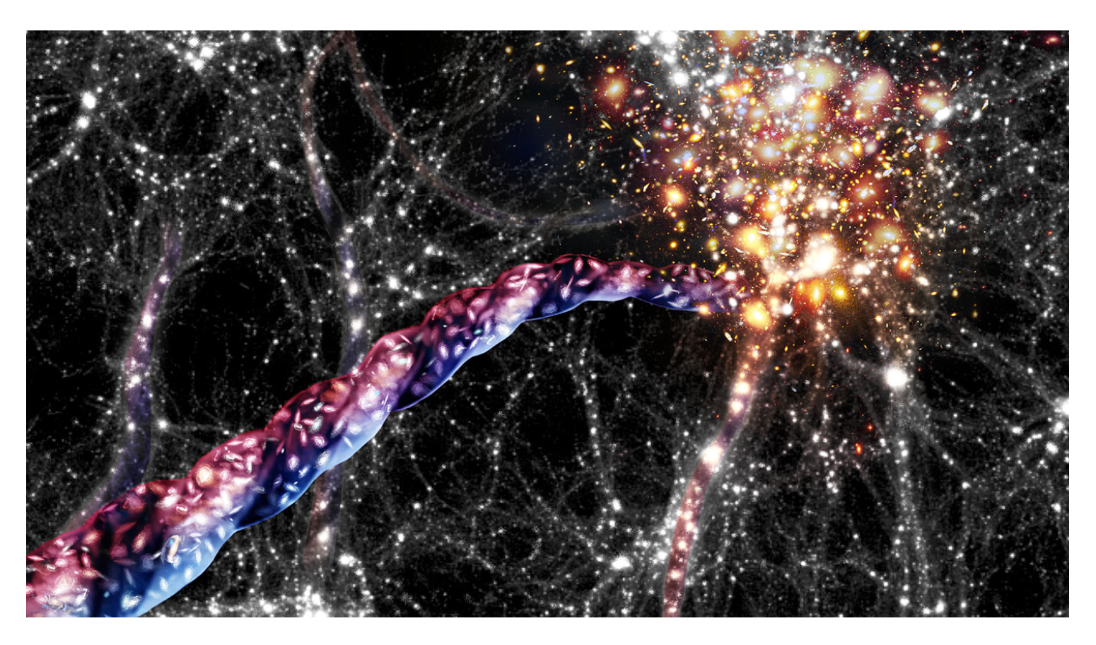
Figure 1. Cosmic Filaments Connecting Galaxies, shown as white dots : Image Source ScienceNewsExplores Cosmic filaments by Jaime Chambers [1].

Figure 1. Cosmic Filaments Connecting Galaxies, shown as white dots : Image Source ScienceNewsExplores Cosmic filaments by Jaime Chambers [1].

Recent updates in PyTorch (version 1.7) have introduced support for complex-valued designs via torch.complex64, and TensorFlow also accommodates numerous libraries that facilitate designs involving complex-valued numbers. Nevertheless, training such networks to achieve comparable performance could require over seven days and involve four times more parameters, which was not pursued in our approach.

In future work, we anticipate that employing complex-valued transformations within upstream CNN layers will effectively suppress image backgrounds, enabling YOLOv8 to accurately detect the structural characteristics of camouflaged objects, even when they blend in with their surroundings in terms of texture, color and edges defining object shape. We intend to explore this direction further.

Our current approach to camouflaged object detection revolves around edge detection and shape separation. The YOLOv8 architecture tends to attenuate edge features as data passes through its layers, necessitating data augmentation to mitigate this effect. While detecting the shapes of camouflaged objects by working within the CVNN domain (Complex Value Neural Networks) could aid in identifying occluded structures, this paper exclusively utilized real-numbered data derived from FtBg.

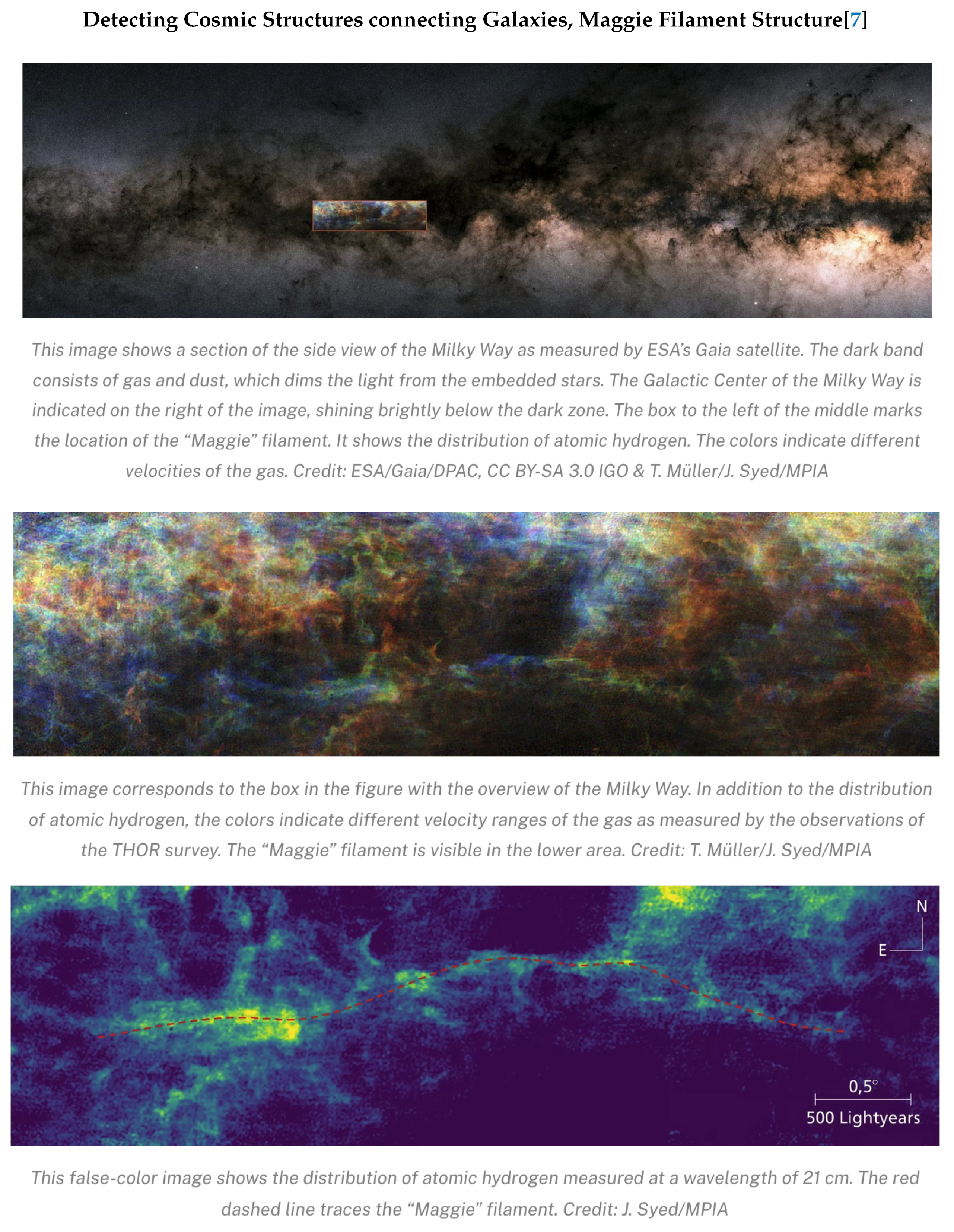
1.2. FtBg [6] Milkyway Filament Separation Approach

Filament structures are large and complex and are often obscured by light noise, infrared radiation from other stars and can only be seen against high contrasting backgrounds in FITS[1] images, following morphological, temperature, and by following the curvature (velocity coherence) [6]

Here is an example of what Astronomers call a "big discovery" a Maggie (named after a river in Colombia by Dr Juan D. Soler) filament, 3900 light years long. FtBg program used data from Herschel Space Observatory [6]. This program uses FFT power spectrum analysis to isolate structures of high contrast by separating regions of low spatial frequency (from high ones), by performing an inverse Fourier Transform. The separation between low and high spatial frequencies is determined from the power spectrum [6]. In our case we set our cutoff threshold to 80 percent instead of what FtBg used as default 90 percent. This is an hyper-parameter for us.

Figure 2. 3900 Light years long Maggie Filament[7]

Figure 2. 3900 Light years long Maggie Filament[7]

1.3. Weaknesses of Other Research Approaches

One of the primary obstacles encountered in the detection of camouflaged objects relates to practical applications of image segmentation techniques deploying pixel level annotations, particularly in object detection tasks targeting camouflaged objects and not utilizing other structural features present in obscured/camouflaged objects. The challenge arises from the inherent nature of using bounding boxes as true labels for camouflaged objects, which introduces a surplus of redundant background information (as at times entire image could contain a large camouflaged object), effectively acting as "noise." Consequently, researchers have encountered difficulties in advancing camouflage detection further while utilizing YOLOv8.

Another complication arises when multiple camouflaged objects cluster together in their natural environments. In future efforts, we intend to utilize spatial separation algorithms like FtBg to extract cluster structures for identifying such objects.

An additional challenge includes the loss of texture information when reducing image dimensions[3,4], needing them to train model with larger images so that more information about hidden features can be extracted.

Our approach addresses these shortcomings by also looking at hidden structures that become visible when signal-processing techniques are deployed, in order to extract information about edges (high-pass filter) and structure (FtBg - milkyway filament extraction algorithm). Data from telescopes arrives in multiple channels carrying information in infra-red and ultraviolet radiation spectrum level "color space" where image is not defined by its edges but by its spectrum. We are feeding this data to YOLO backbone, separating out foreground spectrum from background, requiring no information about "edges" as image and its color-space are really returning waves analyzed through their FFT like spectra (screen stretch [8] is somewhat technical term it).

1.4. Related Work

YOLOv8 with augmented CNNs is currently detecting about 70 percent of the objects in COD10K dataset [9]. Anabranch[10] network for camouflaged object detection [10], reported 66 percent correct identification (segmentation only) as these objects are large, and at time cover, more that 70 percent of picture (Stingray submerged under sandy ocean, large coiled python over dried leaves etc..), YOLOv8 in general, will find these dataset challenging, due to its limitation of not carrying edge features deep into its neural net layers.

2. Dataset

We used Yolov8 small pre-trained model as backbone and then used COD10K and CAMO datasets. We did not pre-process data in any super structured way, just gave it bounding box information that YOLO expects, requiring no human effort of careful labeling. Our Github repository has converter.tgz (FtBg modified for RGB), edge-shape.tgz (highpass filter) scripts used for this work at https://github.com/LilyLiu0719/CS231N-final-project.

2.1. Data Pre-Processing

We utilized CVAT.ai and custom scripts to convert our existing data into YOLO 1.1 format, which includes class labels, center coordinates, width, and height values for object detection. However, we encountered an issue with accurately identifying the centers of bounding boxes containing camouflaged objects using our scripts, leading to lower-than-expected training accuracy due to difficulties in precise bounding box delineation.

While CVAT.AI supports various data formats, creating a custom dataset compatible with YOLOv8 for object detection involves a manual process. Although there are services available that can annotate bounding boxes on our 1250-image CAMO dataset, we opted against using them to gain firsthand familiarity with the data, including different shapes, lighting conditions, and various types of camouflage occlusions in natural settings. This approach allows us to properly augment our data and implement effective strategies for object and shape separation.

We initially explored Roboflow for tagging our camouflaged dataset using the foundational model "grounding DINO," but it successfully tagged non-camouflaged objects while encountering difficulties with camouflaged ones.

Ultimately, we adopted data conversion scripts from the GitHub repository https://github.com/SYED-M-HUSSAIN/COD/, which utilize the imutils Python package to draw bounding boxes based on segmentation masks. This method provided us with a more reliable approach to handling our dataset annotations.

We encountered a challenge with bounding boxes when multiple zebras stood together, where each zebra’s stripes were identified as contours, resulting in incorrect bounding box assignments. To address this issue, we employed PyTorch’s mask-based APIs to draw bounding boxes. This approach was chosen because our dataset already included color labels for each object individually (such as red and green labels).

3. Methodology

3.1. Model Selection

Several recently developed object detection models, including Sparse R-CNN, Anabranch, YOLOv8, and Vision Transformers with mask separable attention, face challenges in real-time detection of occluded camouflaged objects. As precision requirements increase, these models demand more computation time for object classification, resulting in object detection times of up to 20 seconds, albeit with high accuracy. The challenges stem from the dynamic and extensive nature of these objects, often spanning nearly the entire image, which complicates edge detection as there are lot few signals for background and foreground separation .

Our objective is to enhance precision while maintaining low modeling and training costs, enabling exploration of various approaches using datasets like COD10K (accessible at https://dengpingfan.github.io/pages/COD.html) and CAMO (available at https://sites.google.com/view/ltnghia/research/camo).

Full survey of various concealed object detection methods can be found here. https://github.com/ChunmingHe/awesome-concealed-object-segmentation

Figure 3. Results from Zero-Shot Object Detection by Haoran, Li et al (Ours is Heron Li’s data [4], see Table 8 for 3 YOLO.

Figure 3. Results from Zero-Shot Object Detection by Haoran, Li et al (Ours is Heron Li’s data [4], see Table 8 for 3 YOLO.

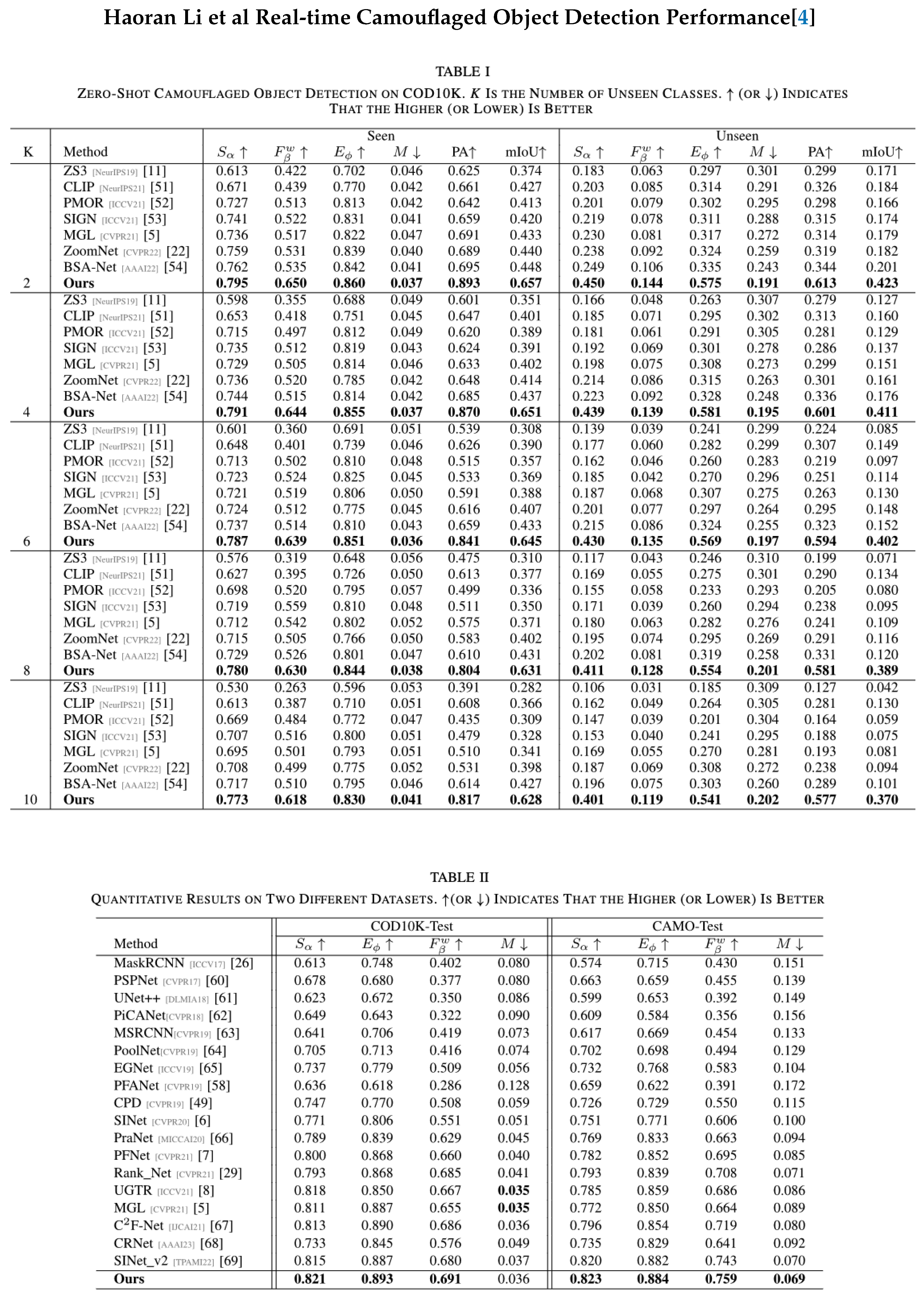
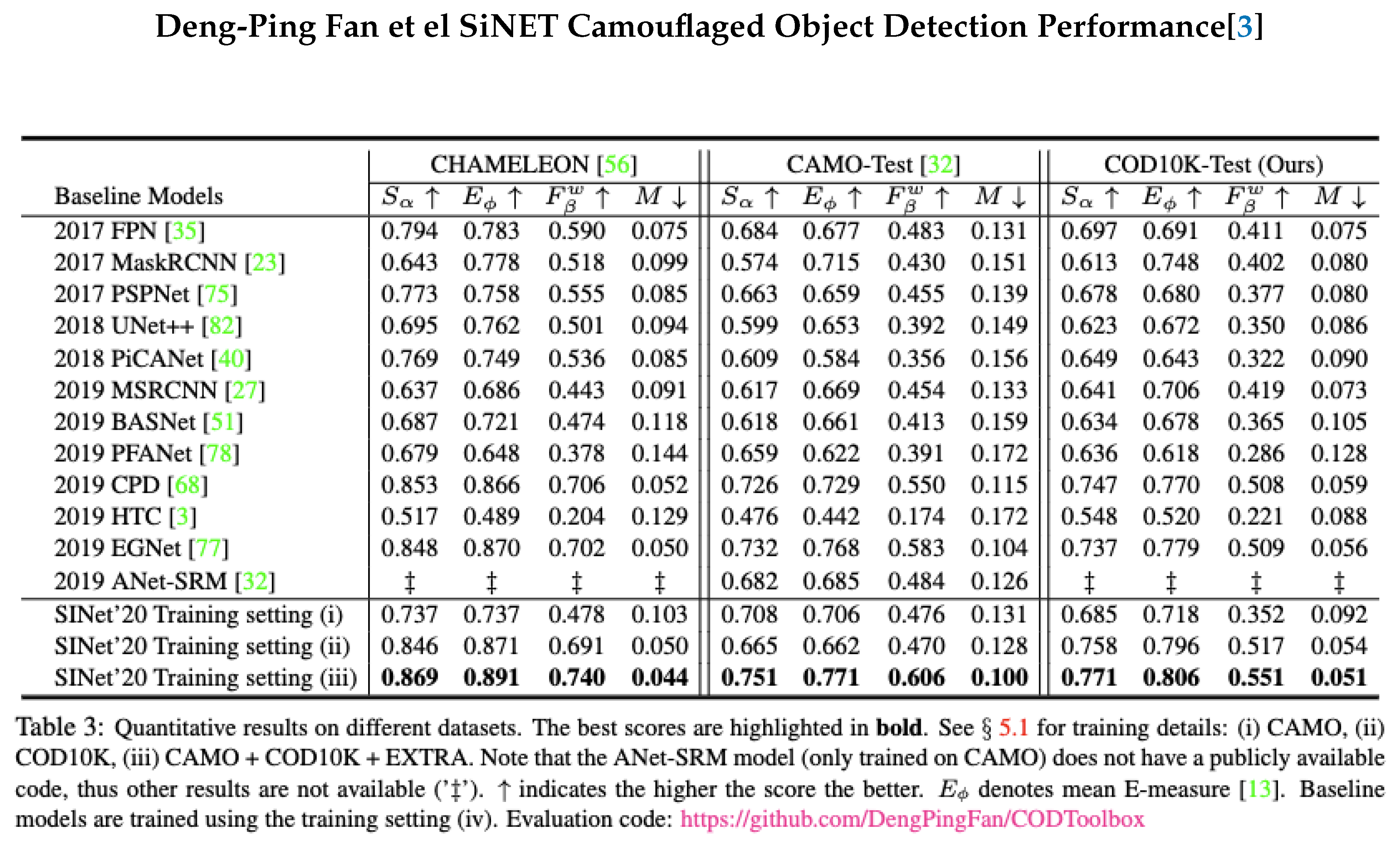
Figure 4. SiNET Performance by Deng-Ping Fan et al[3], see Table 8 for 3 YOLO.

Figure 4. SiNET Performance by Deng-Ping Fan et al[3], see Table 8 for 3 YOLO.

3.2. YOLOv8 Baseline

Pre-trained YOLOv8 model with CAMO dataset, did not perform well, giving only about 3.96% on mAP(50:95). We attribute this to:

1. Smaller model (YOLOv8 nano) not being able to capture occluded, camouflaged edges and shapes and

2. Training with dataset of 152 images.

3.3. YOLOv8 COCO Data Format Alignment

Initially, we trained the YOLOv8x (largest model) for 120 epochs but encountered issues with incorrect bounding box centers, resulting in an average precision of about 18.2

To draw bounding boxes, we initially used the OpenCV findContours method, which proved ineffective for datasets like COD10K. This method inaccurately identified contours, treating each stripe on zebras as separate camouflaged objects, thereby severely impacting our training accuracy, which remained in single digits.

Figure 5. Highlighting failing cases of various bounding box scripting based methods.

Figure 5. Highlighting failing cases of various bounding box scripting based methods.

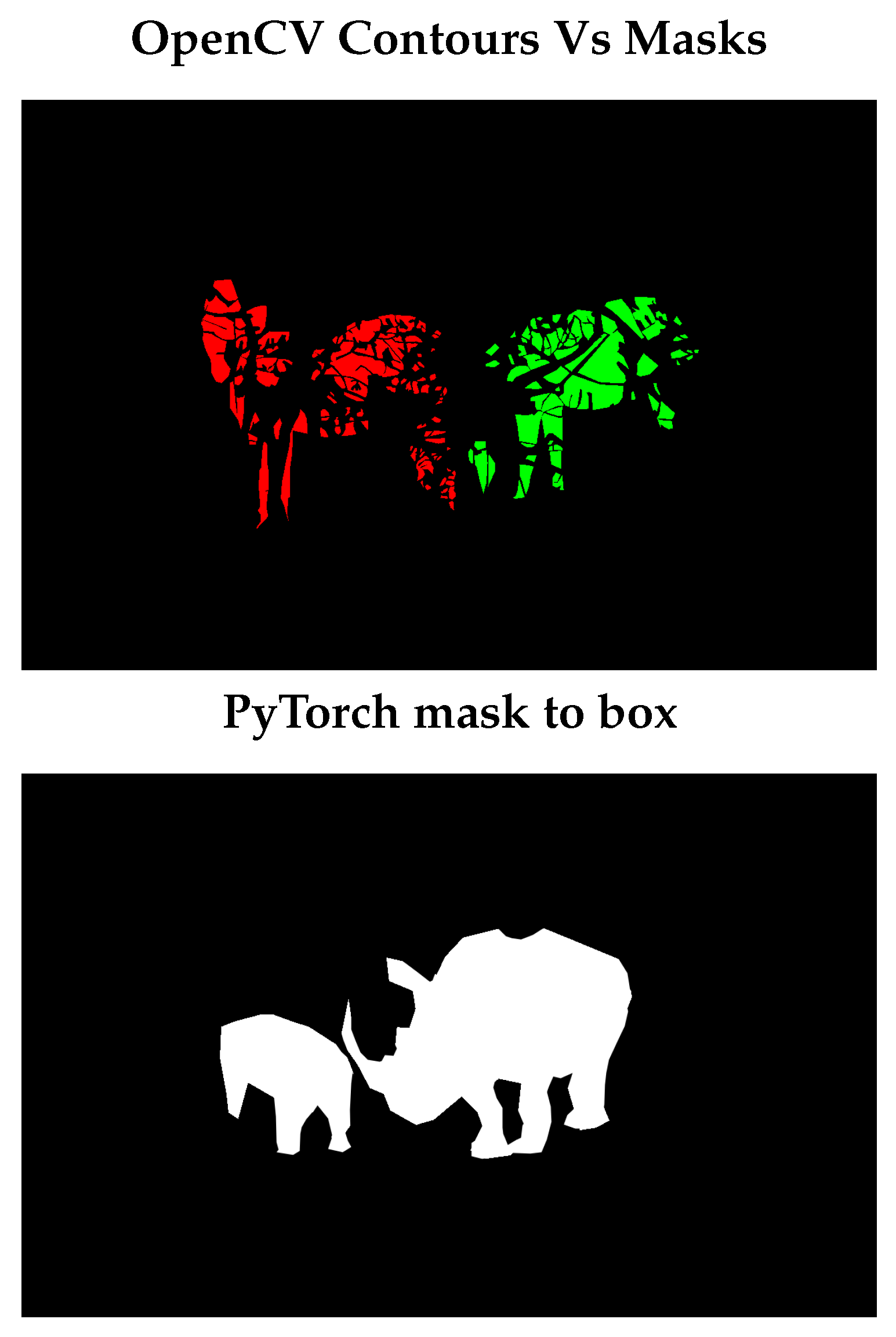
While investigating the YOLOv8s model’s poor performance on the COD10K dataset, we observed that certain label files contained numerous bounding boxes. Training on images with multiple instances was consuming up to 7.8 GB of GPU memory. Specifically, we focused on patched objects such as Giraffes, Zebras, and Shrimps that were failing detection. We used PyTorch method ( torchvision.utils : draw_bounding_boxes ) to draw bounding boxes. Whole process only took few seconds for CAMO and COD10K, compared to 60 minutes/image spent by some approaches such as SiNET, while trying to gain deeper [3] understanding about algorithm.

We identified that the OpenCV findContours method, which worked adequately for simpler objects in the CAMO-COCO dataset (without intricate patterns like stripes), failed to recognize entire objects as single entities. Transitioning to PyTorch’s torchvision.ops "mask to box" method rectified this issue, enabling accurate bounding box generation. Subsequently, we fed these correct bounding boxes into a fresh run of the YOLO pretrained model, resulting in training precision in the range of 50% for mAP50 and 25% for the mAP50-95 metric, similar to the performance achieved on the CAMO-COCO dataset.

Figure 6. Correct Bounding boxes on Patchy objects.

Figure 6. Correct Bounding boxes on Patchy objects.

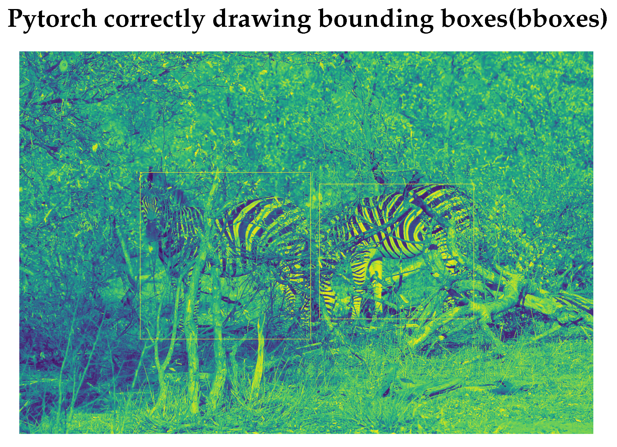
Table 1. YOLO Models Complexity and Performance.

Models	Size	Param.	Speed (ms)	mAP(50:95)
YOLOv8n	640	3.2 M	0.99	37.3
YOLOv8s	640	11.2 M	1.2	44.9
YOLOv8m	640	25.9 M	1.83	50.2
YOLOv8l	640	43.7 M	2.39	52.9
YOLOv8x	640	68.2 M	3.53	53.9

Table 1. YOLO Models Complexity and Performance.

Models	Size	Param.	Speed (ms)	mAP(50:95)
YOLOv8n	640	3.2 M	0.99	37.3
YOLOv8s	640	11.2 M	1.2	44.9
YOLOv8m	640	25.9 M	1.83	50.2
YOLOv8l	640	43.7 M	2.39	52.9
YOLOv8x	640	68.2 M	3.53	53.9

We selected the YOLOv8s model as our foundation to conduct numerous experiments and deliver a solution for performing real-time object detection in field operations, particularly for rescue missions. Our goal is to avoid the lengthy detection times (up to 40 seconds in R-CNNs) required for high precision. This capability is crucial for firefighters and first responders who rely on our model to swiftly respond during rescue missions. Therefore, we prioritize faster speed over absolute accuracy.

3.4. Loss Function

We have opted to design our loss function as a combination of three losses (object detection, edge enhancement and Shape enhancement), mirroring the approach used in the Vision Transformer (ViT) paper for detecting camouflaged objects[11]: https://ieeexplore.ieee.org/stamp/stamp.jsp?tp=&arnumber=10207675. This approach is not yet implemented as we are working on modifying YOLO to have these convolutions upfront, reducing 3 pipelines to one.

1. Classification Loss:

Currently, we are categorizing objects as either camouflaged or non-camouflaged using a single class representation. As we continue refining our datasets for compatibility with YOLOv8, we plan to incorporate fine-grained classification identifiers that represent various object classes.

2. Objectness Loss - based on edge:

This metric determines whether our neural network successfully distinguished the object from its background. This loss quantifies the deviation between our detection and the ground truth bounding box, reflecting the accuracy of our edge detection and shape separation. It encapsulates the effectiveness of our texture pre-processing, achieved through initial CNN layers that apply high-pass filters or wavelet processing to separate the edges and shapes of camouflaged objects from their backgrounds.

3. Regression Loss - Shape:

This loss quantifies the disparity between the predicted class and the true class. In the context of single-class identification, it is equivalent to the classification loss mentioned earlier. However, for multi-class identification, we plan to utilize this loss to accurately differentiate between different categories. It will determine whether our model correctly identifies whether there is a camouflaged bird, insect, or fish in the picture. The same method will also be used to identify multiple objects.

$$L=L_{classification}+L_{object}+L_{regression}$$

3.5. Training Budget

YOLO - A week of training results in 88% accuracy on non camouflaged objects.https://arxiv.org/pdf/1506.02640

ViT - 30 Days of training

Ours - 2 hrs/dataset (< 250 epochs on A100). This constraint enables us to evaluate our model on two distinct datasets: one featuring small objects (CAMO-COCO) and the other comprising larger, more intricate objects. These objects exhibit occlusion, blurred edges, and multiple instances, all under varying lighting conditions and reflections in water. To achieve this evaluation, we employed FFT-based color frequency separation ratios, specifically utilizing a separation ratio of 0.8 for foreground and background spatial frequencies.

3.6. Metrics

We intend to add CNN layers to YOLO model and may transform some layers to transformer like architecture supplying some context about camouflage (such as leaves, trees, occlusion, when edges are blurred, rely on shape by adjusting biases given to prediction coming from shape vs edge based features).

YOLOv8 reports F1 scores and mean average precision mAP50 and mAP(50:95), we intend to keep this metric for our classification.

$$F{1}_{score}={\displaystyle \frac{TP}{TP+\frac{1}{2}(FP+FN)}}$$

$$mAP={\displaystyle \frac{1}{c}}\sum _{K=i}^{N}P\left(K\right).\Delta R\left(K\right)$$

In above equations, TP is True positive, FP is false positive, FN is false negative, c represents object categories, K represents Intersection over Union (IoU) threshold. P(K) is precision and R(K) is recall.

These metrics are standard in object detection and classification literature.

3.7. Transfer Learning

In addition to training the entire YOLO network, we implemented transfer learning by freezing weights in specific layers of the YOLO backbone model while updating the remaining layers using the CAMO dataset. This approach provides an efficient method to fine-tune the YOLO model for detecting occluded objects without requiring high computational resources. We conducted training on a CPU for 50 epochs, totaling 17 hours, using the COD10K CAMO dataset and achieved an mAP50 score of 0.411.

We froze 123 out of 184 layers (15 out of 22 in the module view) in the YOLOv8 nano model, reducing the number of parameters for gradient calculation from 3,157,200 to 1,420,880. This reduction enabled feasible training on CPU machines. The performance of both the transfer learning model and the fully-trained model will be detailed in the results section.

4. Ensemble Learning Using 3 Models

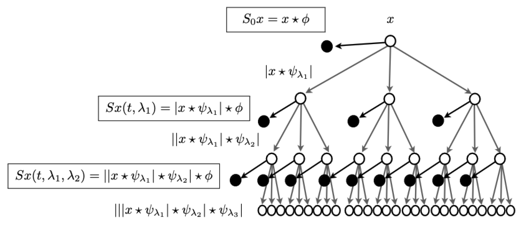
To explore texture information analysis, we aimed to transition to the complex domain using Fourier Transforms. We explored the scattering transform, which is described as a complex-valued convolutional neural network utilizing wavelets as filters. This framework allows certain signals to propagate across longer distances in the network while restricting others to shorter distances, thereby limiting their influence. This approach was chosen based on extensive literature suggesting that texture processing can effectively utilize FFTs[12,13,14]. Wavelet CNNs[15] can be viewed as detailed in the source: https://www.di.ens.fr/data/publications/papers/1304.6763v1.pdf.

We chose not to investigate deeper models [16] because our experiments indicated that, despite a fourfold increase in training budgets, the improvement in accuracy was marginal when using Yolo Large/X-Large models.

We observed improved results by separating the foreground and background through FFT-based texture processing for camouflaged objects[17].

Figure 7. Wavelets traversing CNNs, source: https://www.di.ens.fr/data/publications/papers/1304.6763v1.pdf.

Figure 7. Wavelets traversing CNNs, source: https://www.di.ens.fr/data/publications/papers/1304.6763v1.pdf.

Pytorch has support for complex valued tensors and YOLOv5 has a port supporting complex valued CNNs.

We investigated use of direct cosine transforms for camouflage detection as outlined in https://openaccess.thecvf.com/content/CVPR2022/papers/Zhong_Detecting_Camouflaged_Object_in_Frequency_Domain_CVPR_2022_paper.pdf to separate foreground and background distances, however we realized that biggest gains in highly camouflaged objects were made by edge enhancements and shape separations (specially for human shapes with buildings in background).

These approaches employed modified loss functions that utilized discrete cosine transform (DCT) based norms instead of Euclidean norms to determine whether a given image tile resembled or differed from others, thereby enabling camouflaged object detection. These changes also necessitated adjustments in the dot product implementation and softmax function, requiring a complete retraining of the network since the pre-trained weights from the YOLOv8s model were not directly applicable.

Due to our restricted seven-day training budget, we opted to integrate insights from space image data processing. Specifically, we utilized only the real part of complex numbers after FFT operations for image refinements.

We developed three YOLOv8s models to facilitate ensemble learning. One operated in base mode using the dataset as provided. Another specialized in edge detection by employing high-pass filters, while the third focused on shape detection by separating high and low spatial frequencies in the Fourier domain, inspired by techniques used in processing data from space telescopes[6] (source: https://arxiv.org/pdf/1504.00647). Initially, we planned to apply these filters as convolutions in the complex domain throughout the YOLO architecture. However, we found that processing the real part of numbers was sufficient to increase mAP50 and mAP(50:95) scores by 10 percentage points when using shape-related wavelet transforms with tuned hyper-parameters. Our approach utilized YOLOv8s and YOLOv8n models, acknowledging their limitations in expressing complex features.

Table 2. High Pass filter transform, extracting edges, Original image is on left, extracted edges are on the right.

Table 2. High Pass filter transform, extracting edges, Original image is on left, extracted edges are on the right.

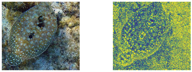
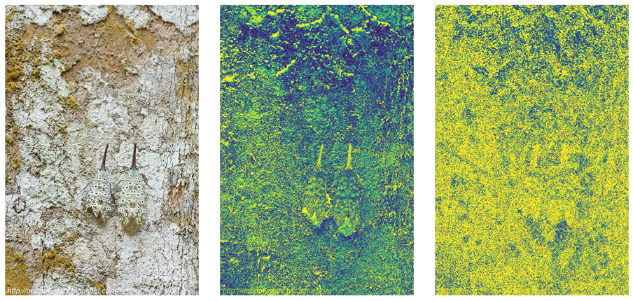
The third model explored two approaches. Initially, we implemented the Kymatio wavelet scattering network (available at https://www.kymat.io/), which is differentiable, allowing these layers to be integrated into the general YOLO pipeline. This approach generated two sets of Scattering2D coefficients aimed at enhancing object shape detection (refer to Table 2 above). However, we encountered significant computational challenges with these wavelet transforms when running on CPU, taking between 20 to 30 seconds per image on a machine with 56 cores.

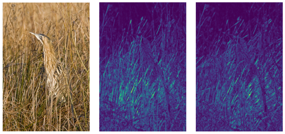
Table 3. Scatter2D wavelet differentiable transforms. Original heron image (L), Scatter2D transform with scatter scattering coefficient=1 (M), Scatter2D transform with scatter scattering coefficient=2 (R).

Table 3. Scatter2D wavelet differentiable transforms. Original heron image (L), Scatter2D transform with scatter scattering coefficient=1 (M), Scatter2D transform with scatter scattering coefficient=2 (R).

We attempted to utilize GPU acceleration, but encountered instability with the CuPy package necessary for GPU processing. This instability caused the system to crash twice, resulting in complete data loss due to CUDA version mismatches between PyTorch 11.8 and CuPy 12.2. Consequently, we decided to discontinue the use of wavelet Scattering2D for this application.

Our primary objective remains real-time detection of camouflaged objects to support firefighters and other emergency responders. This capability is essential for integrating such systems into head-up displays, enabling quick identification of individuals in scenarios involving smoke, underwater conditions, or other visually challenging environments.

We then embarked on extracting shape information using foreground/background processing, using Ftbg algorithm https://ui.adsabs.harvard.edu/abs/2017ascl.soft11003W/abstract. We converted the package to handle images in .jpg and .png format as it only handled images in FITS format as most of the data from space telescopes comes in, in this format or processed in this format.

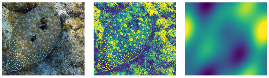
Table 4. Fourier Transforms isolating foreground (structure), by separating high spatial signals from low ones. Original, Enhanced foreground, leftover background.

Table 4. Fourier Transforms isolating foreground (structure), by separating high spatial signals from low ones. Original, Enhanced foreground, leftover background.

We produced predictions in all 3 models separately and then looked at failing cases in base models, to check whether FFT/wavelet processing could have helped in further detection, from other two models. We found out that in some cases, shape detection produced camouflaged object detection, where other two methods have failed.

We also found that edge detection triggered camouflaged object detection with low IOU (i.e. bounding box was away from the object).

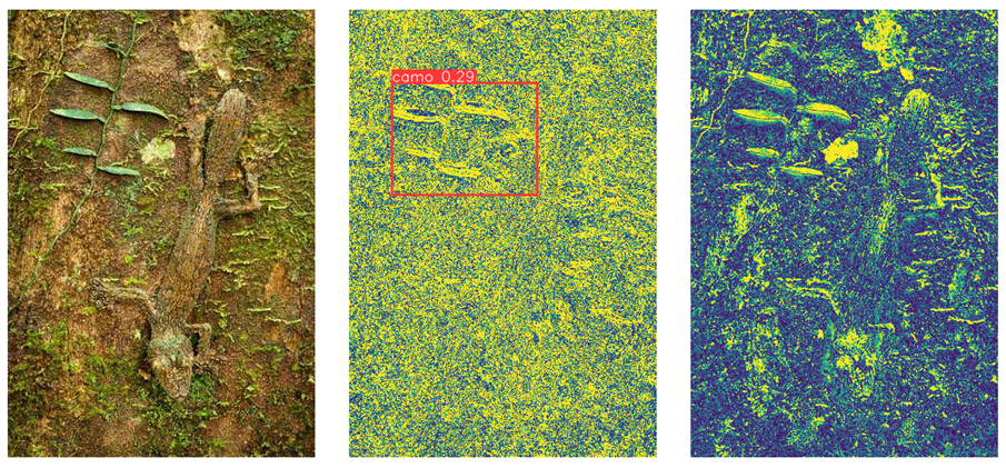
Table 5. Edge enhanced CAMO object detection, 3rd picture shows shape based detection failed.

Table 5. Edge enhanced CAMO object detection, 3rd picture shows shape based detection failed.

We also noticed that shape based detection, increase our mAP50 to 0.56 and mAP(50:95) to 0.30 from earlier mAP50 of 0.5 and mAP(50:95) of 0.25.

We intend to combine all the models to create one final prediction as we noticed that each model has its own strengths in isolating camouflaged objects where other two might have failed.

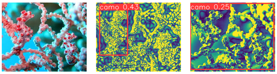
Table 6. Ensemble Model detecting camouflaged object, Model that did not use fourier transforms failed to detect camouflage object, other two models (Edge enhanced, Shape enhanced) were able to detect. Edge enhanced did best.

Table 6. Ensemble Model detecting camouflaged object, Model that did not use fourier transforms failed to detect camouflage object, other two models (Edge enhanced, Shape enhanced) were able to detect. Edge enhanced did best.

5. A comparison of YOLO Architectures

YOLOv1 - Single CNN to perform real time object detection, by dividing image into GRID, making multiple predictions about existence of an object and then picking one with highest probability after removing overlapping boxes.

YOLOv2 - Darknet-19 backbone, used anchor boxes idea from Faster R-CNN and batch norm in all its convolution layers, increasing prediction accuracy.

YOLOv3 - Darknet 53 backbone, utilizing residual connections, up-sampling and logistic classifiers achieving 3x speed with comparable accuracy to RetinaNet.

YOLOv4 - This YOLO deployed spatial attention.

YOLOR - Added 2 pipelines to provide explicit knowledge and implicit knowledge to Discriminator thus adding capability to handle multiple tasks.

YOLOX - Deployed Anchor Free, CIOU loss giving moderate increase in precision. CIOU loss not only penalizes incorrect bounding box co-ordinates but also considers the aspect ratio and center distance of the box.

Table 7. CAMO-COCO and COD10K Dataset Validation-Set Results, Fine tuned YOLO, without edge and shape enhanced additions.

Dataset	Img.	Box(P	R	mAP50	mAP(50+)
	Val
CAMO	250	0.58	0.468	0.473	0.211
COD10K	2026	0.655	0.481	0.52	0.255

Table 7. CAMO-COCO and COD10K Dataset Validation-Set Results, Fine tuned YOLO, without edge and shape enhanced additions.

Dataset	Img.	Box(P	R	mAP50	mAP(50+)
	Val
CAMO	250	0.58	0.468	0.473	0.211
COD10K	2026	0.655	0.481	0.52	0.255

YOLOv6 - Deployed DIOU loss. Distance IOU loss incorporates normalized distance between the predicted box and the target box which converges much faster than generalized IOU (GIOU) loss.

YOLOv7 - Added Leaky ReLU activation and CSPDartnet-Z Backbone. CSPNet partitions the feature map of base layer into two parts and then merges them through a cross stage hierarchy. Use of split and merge allows for more gradient to flow through the network, giving 1% increase in mAP.

YOLOv8 - This adds Exponential Linear Unit (ELU) for activation, multi-scale object detection and new backbone architecture called CSPDarkNet + C2F module which combines high level features with contextual information. ELU is added to address vanishing gradient problem using CIOU and DFL (Binary cross entropy for classification loss) loss (over Generalized Intersection over Union loss https://giou.stanford.edu/) addressing how close shapes are to each other (i.e if no intersection, so intersection over union (IOU) is not helpful), central point difference between predicted box and ground truth and aspect ratio difference in predicted box to ground truth box. https://encord.com/blog/yolo-object-detection-guide/, https://arxiv.org/html/2304.00501v6.

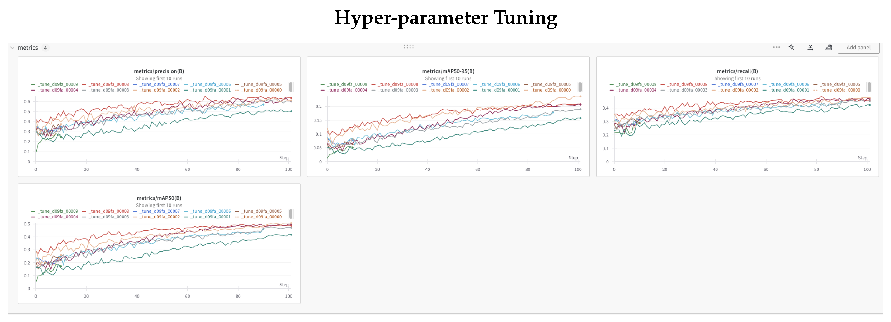
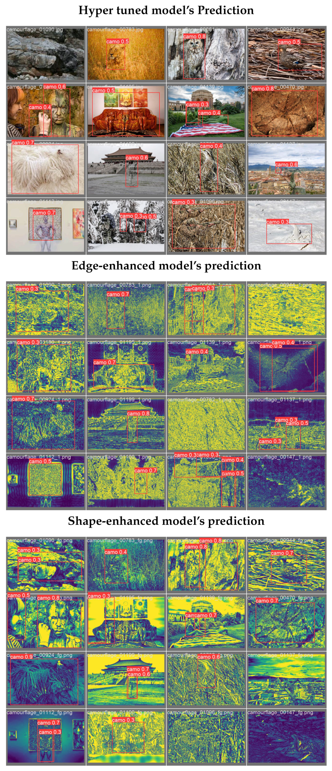
6. Hyper Parameter Tuning

We used Ray-Tune and Weights and Biases to fine tune our model. Ray-tune performed a grid search, on 30 or so available YOLO hyper parameters, resulting in most optimal set after running for 100 epochs. These runs are very costly as they run for typically 6-8 hours on NVIDIA Dual A100 GPUs.

We then used these best hyper-parameters to further train/tune our shape and base models.

Figure 8. Ray-tune and Weights and Bias based hyper parameter tuning for 100 epochs

Figure 8. Ray-tune and Weights and Bias based hyper parameter tuning for 100 epochs

7. Results/Evaluation

We trained YOLOv8s (pretrained) using CAMO dataset for 289 epochs and then used this trained model on COD10K dataset for 500 epochs.

Figure 9. base line model prediction example after training for 500 epochs

Figure 9. base line model prediction example after training for 500 epochs

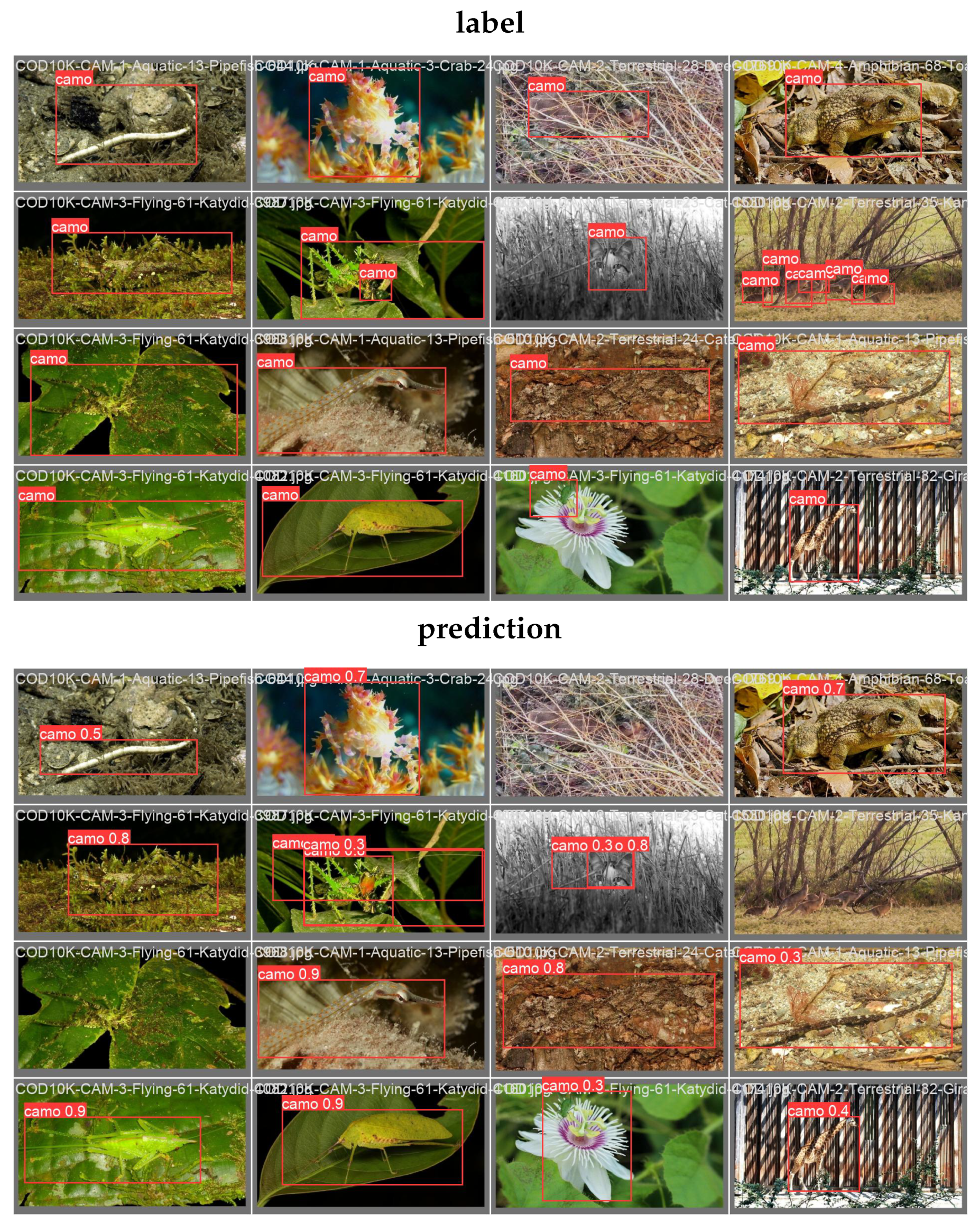
We have been experimenting with various features on model performance to fine-tune the best approach.

We achieved 50 % accuracy (mAP50) on both of these datasets.

We conducted training on the CAMO-COCO dataset for 289 epochs followed by further training on the COD10K dataset for 500 epochs. This approach resulted in achieving a validation set accuracy of 50% for mAP50 and 25% for mAP(50-95). Interestingly, we observed nearly identical results on both datasets, despite challenges with the YOLO model’s performance on large objects where the bounding box spans the entire image. We also trained YOLO for background information by passing background images coming without bounding boxes using Milkyway filament extraction based foreground, background separation algorithm. See detailed results in Table 8 below.

Ensemble Learning by Feature Fusion

We integrate weights from multiple models by combining them equally before making predictions. YOLO facilitates this integration through APIs that enable feature fusion from different models (source: https://github.com/ultralytics/yolov5/issues/7905).

Table 8. Incremental Performance increase.

Model	mAP50	mAP(50:95)	#p(M)
Pretrained YOLOv8s	0.0396	0.076	11.2
Finetuned YOLOv8s	0.520	0.655	11.2
Transfer learning	0.411	0.180	3.2
Edge-enhanced	0.441	0.232	11.2
Shape-enhanced-Hyper	0.556	0.309	11.2
3 YOLO (F + E + S)	0.888

Table 8. Incremental Performance increase.

Model	mAP50	mAP(50:95)	#p(M)
Pretrained YOLOv8s	0.0396	0.076	11.2
Finetuned YOLOv8s	0.520	0.655	11.2
Transfer learning	0.411	0.180	3.2
Edge-enhanced	0.441	0.232	11.2
Shape-enhanced-Hyper	0.556	0.309	11.2
3 YOLO (F + E + S)	0.888

Table 9. Comparison of CAMO Object detection using YOLO, Highpass Filters and Milkyway Filament based structure isolation schemes.

Table 9. Comparison of CAMO Object detection using YOLO, Highpass Filters and Milkyway Filament based structure isolation schemes.

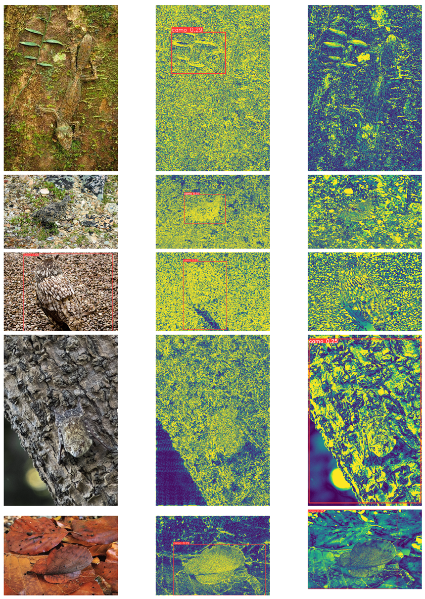
Table 10. Comparison of CAMO Object detection using YOLO (failed), Highpass Filters and Milkyway Filament based structure isolation schemes.

Table 10. Comparison of CAMO Object detection using YOLO (failed), Highpass Filters and Milkyway Filament based structure isolation schemes.

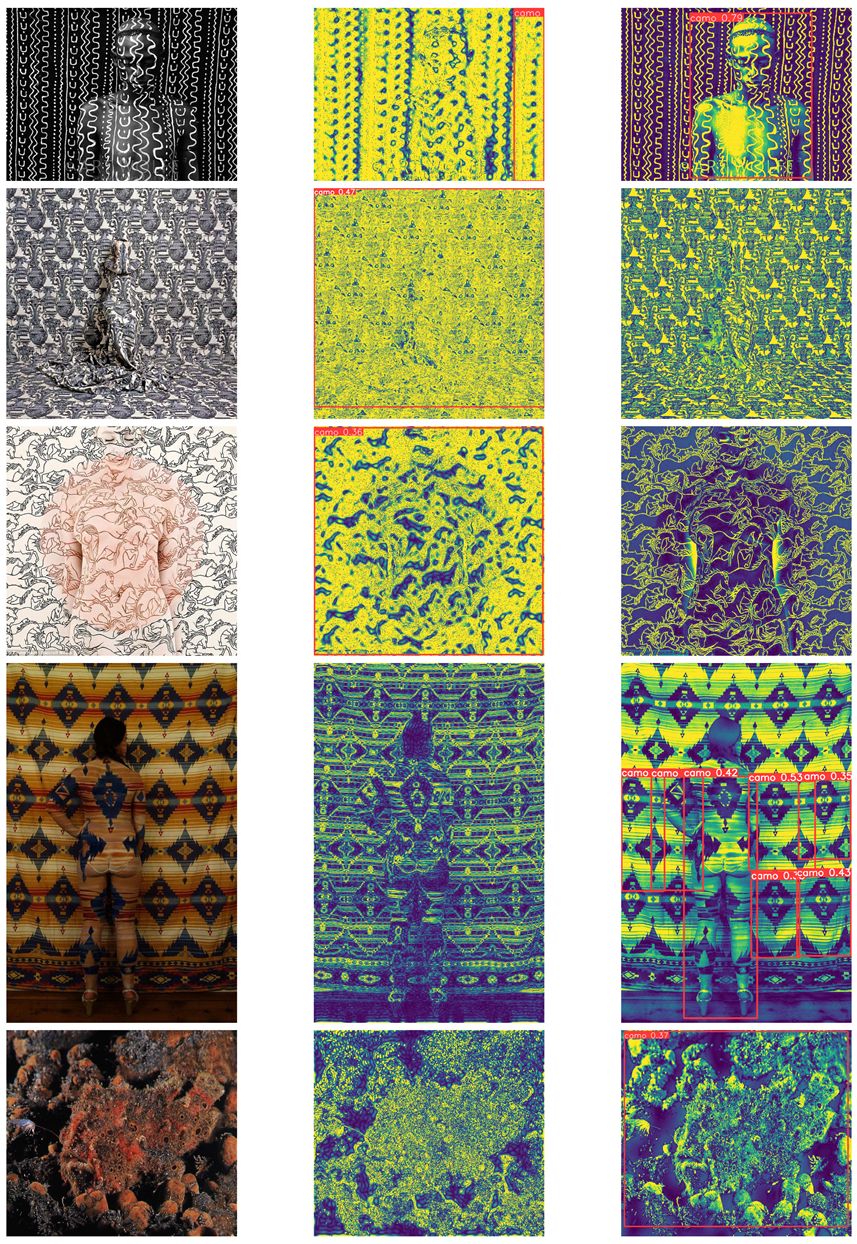
Table 11. Comparison of CAMO Object detection using YOLO (failed), Highpass Filters and Milkyway Filament based structure isolation schemes.

Table 11. Comparison of CAMO Object detection using YOLO (failed), Highpass Filters and Milkyway Filament based structure isolation schemes.

Figure 10. Ensemble Model for Feature fusion based prediction

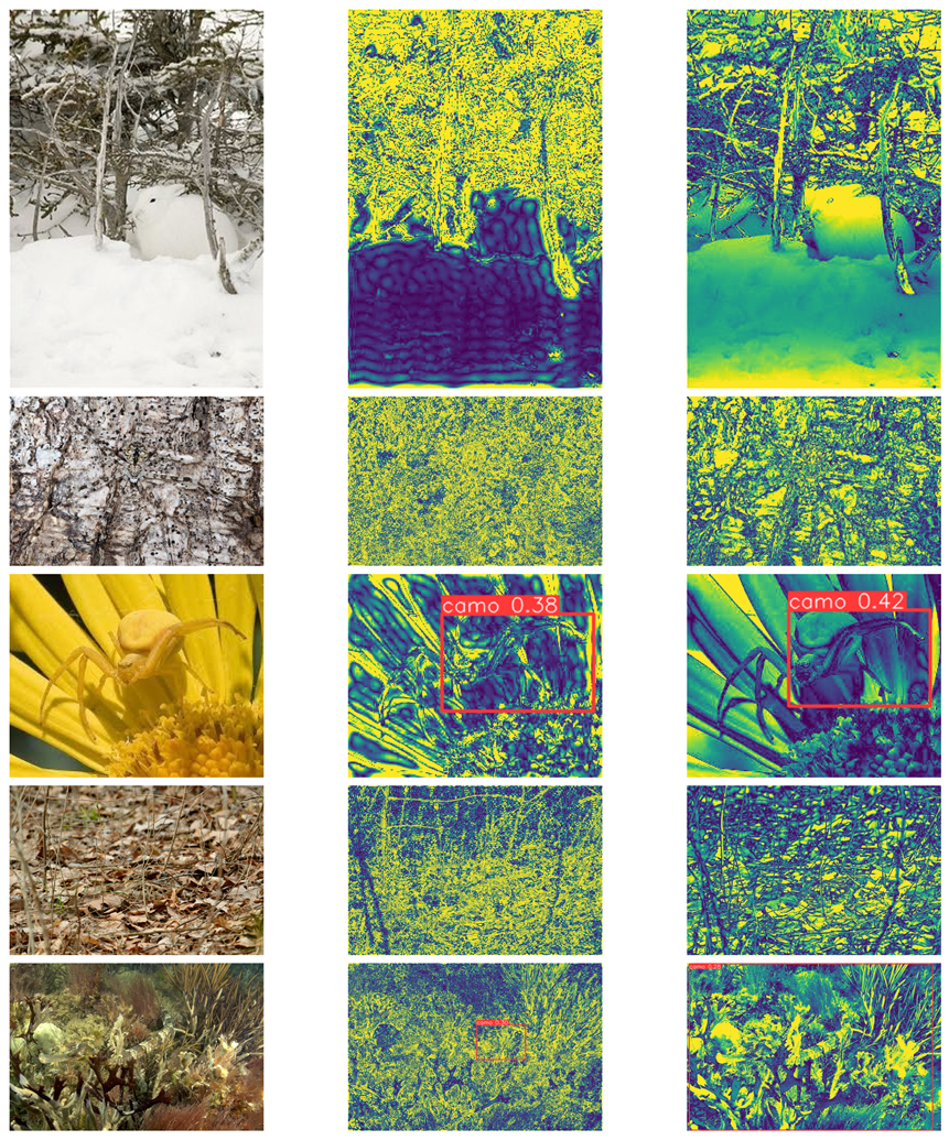
Figure 10. Ensemble Model for Feature fusion based prediction

Transfer Learning

For the transfer learning model, we conducted training on the COD10K dataset for 50 epochs using a pretrained YOLO nano model. This approach yielded a mean precision of 41% (mAP50) on the validation set. While slightly lower than training the entire model from scratch, this method notably enhances the performance of the original pretrained model. Given considerations such as computational cost, model size, training data availability, and time constraints, these results underscore the feasibility and effectiveness of employing transfer learning with a pretrained YOLO model on constrained devices and limited training resources.

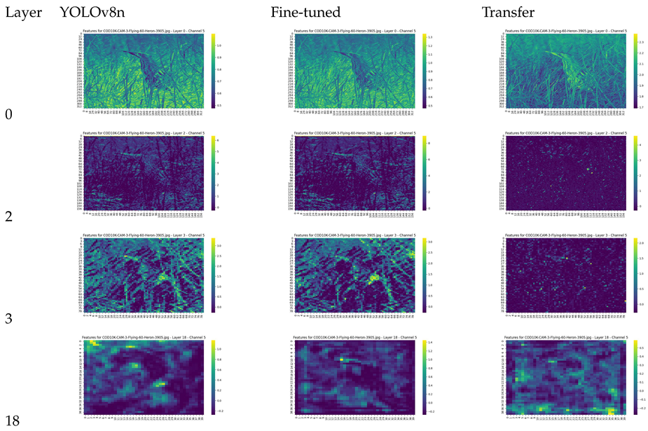
7.1. Feature Visualization

To gain a deeper understanding of how object detection works for camouflaged objects, we implemented feature map visualization on the convolution layers in YOLO models.

The backbone network of the YOLOv8 nano and small models consists of 22 convolution layers. We sampled feature maps from the output of several layers to compare the differences between the models See Fig 10.

Table 12. Test image of hidden heron and prediction, last image is shape enhanced with 0.8 fg/bg spatial frequency separation.

Table 12. Test image of hidden heron and prediction, last image is shape enhanced with 0.8 fg/bg spatial frequency separation.

Table 13. Feature Map Visualization.

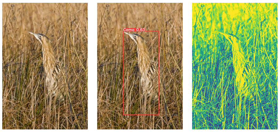
Table 13. Feature Map Visualization.

8. Failing Cases

YOLO does not do well when multiple objects are clustered together. This issue can only be fixed by applying multiple dense layers at the start of neural net to extract relevant features as reported by SINethttps://github.com/DengPingFan/SINet?tab=readme-ov-file See Fig 11 below.

Table 14. YOLO fails to detect multiple objects (Fine-tuned, Edge enhanced, Shape Enhanced).

Table 14. YOLO fails to detect multiple objects (Fine-tuned, Edge enhanced, Shape Enhanced).

9. Conclusions

We believe we have a straightforward solution for a head-up display capable of detecting occluded and camouflaged objects by employing cost-effective transformations. These transformations are adaptable across different environments for various rescue missions. Drawing inspiration from wavelet transforms used to enhance space telescope images of the Milky Way, we can directly apply similar techniques to identify camouflaged objects without incurring the high computational overhead associated with Scatter2D wavelet transforms.

10. Future Direction

We want to explore wavelet transforms and its integration paths into the YOLO framework to facilitate real-time object detection while adhering to low training budgets. This approach combines long-chain wavelet transforms with short-chain convolutions. We aim to leverage FFT transforms to extract textural information and evaluate the similarity among different image patches, akin to methods used in ViT vision transformers. Simultaneously, a traditional convolutional network will utilize the GIOU-based loss function to detect camouflaged objects effectively.

References

- Khalatyan, J.C. Cosmic Filaments may have the biggest spin in outer space. ScienceNewsExplores 2021, 8. [Google Scholar]
- Iris Santiage-Bautiste, César A. Caretta2, H.B.A.E.P. Identification of filamentary structures in the environment of superclusters of galaxies in the Local Universe. Astronomy and Astrophysics 2020, 637, 26. [Google Scholar] [CrossRef]
- Deng-Ping Fan, G.P.J. Camouflaged Object Detection. CVPR 2020, http://dpfan.net/Camouflage/ 2020, 1. [Google Scholar]
- Haoran Li, Chun-Mei Feng, Y. X. Zero-Shot Camouflaged Object Detection. IEEE TRANSACTIONS ON IMAGE PROCESSING 2023, 32, 5126–5136. [Google Scholar] [CrossRef] [PubMed]
- Joshua Bassey, X.L. A survey of Complex Valued Neural Networks. ARXIV https://arxiv.org/pdf/2101.12249 2021, 2101, 234–778. [Google Scholar]
- Ke, W. Large-scale filaments associated with Milky Way spiral arms. https://ui.adsabs.harvard.edu/abs/2015MNRAS.450.4043W/abstract 2015, 1. [Google Scholar]
- Dr. Markus Nielbock, J.S. Raw Material for New Stars. Max-Planck-Gesellschaft, https://www.mpg.de/17979140/raw-material-for-new-stars 2021, 12. [Google Scholar]
- Jr. , R.S.W. Astro-Imaging: Stretching the Truth. Sky & Telescope, https://skyandtelescope.org/astronomy-blogs/imaging-foundations-richard-wright/astro-imaging-stretch/ 2019, 2. [Google Scholar]
- Han, T. Improving the Detection and Position of Camouflaged Objects in YOLOv8. MDPI Electronics 2023, 12, 234–778. [Google Scholar] [CrossRef]
- Le, T.N. Anabranch network for camouflaged object segmentation. Computer Vision and Image Understanding 2019, 184, 45–56. [Google Scholar] [CrossRef]
- Rohan Putatunda, M.A.K. Vision Transformer-based Real-Time Camouflaged Object Detection System at Edge. 2023 IEEE International Conference on Smart Computing 2023, 1, 234–778. [Google Scholar] [CrossRef]
- Joakim Anden, S.G.M. Deep Scattering Spectrum. Transactions on Signal Processing 2014, 2014. [Google Scholar] [CrossRef]
- Mardani, M. Neural FFTs for Universal Texture Image Synthesis. NeurIPS 2020, 2020. [Google Scholar] [CrossRef]
- Aittala, M. Reflectance moideling by neural texture synthesis. ACM Transactions on Graphics (ToG) 2016, 35, 1–13. [Google Scholar] [CrossRef]
- Mallat, S.G. A Theory for Multiresolution Signal Decomposition: A Wavelet Representation. IEEE Transactions On Pattern Analysis and Machine Intelligence 1989, 11. [Google Scholar] [CrossRef]
- Karen Simonyan, A.Z. Very Deep Convolutional Networks For Large-Scale Image Recognition. ICLR 2015, 0. [Google Scholar]
- Yun Wang, P.H. Comparisons between fast algorithms for the continuous wavelet transform and applications in cosmology: the 1D case. RAS Techniques and Instruments 2023, 2. [Google Scholar] [CrossRef]
Disclaimer/Publisher’s Note: The statements, opinions and data contained in all publications are solely those of the individual author(s) and contributor(s) and not of MDPI and/or the editor(s). MDPI and/or the editor(s) disclaim responsibility for any injury to people or property resulting from any ideas, methods, instructions or products referred to in the content. |
© 2025 by the authors. Licensee MDPI, Basel, Switzerland. This article is an open access article distributed under the terms and conditions of the Creative Commons Attribution (CC BY) license (http://creativecommons.org/licenses/by/4.0/).
Copyright: This open access article is published under a Creative Commons CC BY 4.0 license, which permit the free download, distribution, and reuse, provided that the author and preprint are cited in any reuse.