Submitted:
19 June 2024
Posted:
20 June 2024
You are already at the latest version
Abstract
This paper presents the fabrication and characterization of cylindrical capacitors utilizing magnetodielectric materials composed of magnetizable microfibers dispersed within a silicone oil matrix. The microfibers, ranging in diameter from 0.25 to 2.20 μm, comprise hematite (α-Fe2O3), maghemite (γ-Fe2O3), and magnetite (Fe3O4). The study investigates the electrical behavior of these capacitors under the influence of an external magnetic field superimposed on a medium-frequency alternating electric field, across four distinct volume concentrations of microfibers. Electrical capacitance and resistance measurements are conducted every second over a 60-second interval, revealing significant dependencies on both the quantity of magnetizable phase and the applied magnetic flux density. Furthermore, the temporal stability of the capacitors’ characteristics is demonstrated. The obtained data are analyzed to determine the electrical conductance and susceptance of the capacitors, elucidating their sensitivity to variations in microfiber concentration and magnetic field strength. To provide theoretical insight into the observed phenomena, a model based on dipolar approximations is proposed. This model effectively explains the underlying physical mechanisms governing the electrical properties of the capacitors. These findings offer valuable insights into the design and optimization of magnetodielectric-based capacitors for diverse applications in microelectronics and sensor technologies.
Keywords:
electrical capacitors
; silicone oil
; iron oxide microfibers
; magnetic field
; electrical conductance
; electrical susceptance
1. Introduction
Advancements in capacitor technology are pivotal for the development of modern electronic devices and systems [1,2,3,4,5]. Electrical capacitors are essential components in a wide range of applications, from energy storage systems [6,7,8] to advanced sensors [9,10,11] and transducers [12,13,14]. The performance and functionality of capacitors are significantly influenced by the properties of the dielectric materials used, which has led to ongoing research and innovation in this field [15,16]. They form components of an electrical circuit that consist of two or more electrodes with a dielectric material placed between them.
Various types of electrical capacitors are known, each defined by the dielectric material used. For instance, some capacitors utilize dielectric materials such as oil-impregnated paper [17], mineral oil [18], or nonlinear dielectric materials [19,20]. Another category includes electrolytic capacitors, where both the electrodes and the dielectric material are produced using nanotechnology processes [21,22]. These capacitors are specifically designed for storing electrical energy [23]. Additionally, there are capacitors based on silicon oil (SO) and magnetizable nano-microparticles. In these capacitors, the equivalent electrical components can be adjusted magnetically [24,25,26,27,28].
Andrei et al. [24], manufactured capacitors using suspensions based on SO, iron microparticles, and stearic acid with varying mass ratios. These capacitors are characterized by an increase in electrical conductance with the increase in the ratio of stearic acid to the magnetizable phase in a magnetic field. Conversely, the duration for establishing electrical conduction decreases slightly with the increasing intensity of the applied magnetic field. The capacitors detailed in Refs. [25,26] are based on commercially available cotton fabrics impregnated with liquid suspensions that include carbonyl iron microparticles and varying ratios of honey and turmeric powder. When studied in an alternating electric field with frequencies ranging from 25 Hz to 1 MHz, superimposed on a static magnetic field, the equivalent electrical capacitance and resistance of the capacitors are measured. These properties are coarsely adjusted by the ratios of honey to turmeric powder and the values of magnetic flux density, while fine adjustments are achieved through the frequency of the alternating electric field. The capacitors described by Bica et al. [27] are constructed from medical-grade cotton gauze impregnated with liquid composites containing multifloral honey, carbonyl iron microparticles, and varying amounts of turmeric powder. In these capacitors, electrical conductance is coarsely adjusted by the ratio of honey to turmeric quantities and finely tuned by the intensity of the electric field. Iacobescu et al. [28] produced capacitors using cotton fabric impregnated with a magnetic liquid based on mineral oil and magnetite nanoparticles. By maintaining a constant quantity of magnetic liquid, it was observed that the electrical conductance of the composite can be coarsely adjusted by applying compressive stress and finely tuned by the values of the magnetic flux density.
Following this research direction, the present study describes the manufacturing method of capacitors based on SO and microfibers containing -FeO, -FeO, and FeO. The study investigates the electrical behavior of these capacitors under the influence of an external magnetic field superimposed on an alternating electric field, across four distinct volume concentrations of microfibers. Electrical capacitance and resistance measurements are conducted every second over a 60-second interval, revealing significant dependencies on both the quantity of magnetizable phase and the applied magnetic flux density. The obtained data are analyzed to demonstrate that in a medium-frequency electric field, both electrical conductance and susceptance can be coarsely adjusted by varying the ratio of SO to microfibers and finely tuned by the magnetic flux density. Compared to the capacitors produced in [24,25,26,27,28], this study shows that the presence of semiconductor iron oxides in the microfibers alters the behaviour of electrical conductance when a magnetic field is applied. A theoretical model based on dipolar approximations is proposed to explain the underlying physical mechanisms governing the electrical properties of the capacitors.
By providing valuable insights into the design and optimization of magnetodielectric-based capacitors, our findings can influence the development of advanced microelectronic devices and sensor technologies. Improved capacitors with adjustable electrical properties have the potential to enhance the performance and efficiency of energy storage systems, leading to more reliable and scalable renewable energy solutions. Additionally, the ability to fine-tune the electrical characteristics of capacitors through magnetic fields can lead to innovations in electronic circuits, allowing for more adaptable and multifunctional electronic components. This research contributes to the advancement of composites based on iron microfibers and SO, paving the way for new applications and improvements in existing technologies.
This paper is structured as follows: Section 2 provides a detailed description of the materials and methods used in the study, including the preparation of magnetodielectric materials and the manufacturing process of electrical capacitors. Section 3 presents the results of the experimental investigations, analyzing the dependencies of electrical capacitance, resistance, conductance, and susceptance on the volume concentration of microfibers and the applied magnetic flux density. Section 4 discusses the implications of the findings, comparing them with previous studies and theoretical models. Finally, Section 5 concludes the paper by summarizing the key outcomes and suggesting potential directions for future research. The appendices provide additional technical details and supporting data for the experimental and theoretical analyses conducted in the study.
2. Materials and Methods
2.1. Preparation of Magnetodielectric Materials
The materials used for preparation of the magnetodielectric materials are the following:
- SO, from Silicone Comerciale SpA (Italia), with a mass density of g/cm and dynamic viscosity mPa·s at K.
- The iron oxide microfibers (mFe) are obtained in microwave microplasma, following a procedure described in Ref. [29]. They contain oxides of the type (12 % by mass), (62 % by mass), and (26 % by mass). The mass density of the microfibers is at and they exhibit a specific saturation magnetization, A·m/kg, at a magnetic field intensity, . A structural analysis of these microfibers based on SEM, is presented in Appendix A. The average diameter of the nano-microparticles in the microfibers is (see Figure A1).
The magnetodielectric materials consist of mixtures of mFe and SO at four different concentrations, in the form of composite liquids (CL), as listed in Table 1. Each mixture () is mechanically homogenized for a duration of about 300 s at a temperature K. The homogenization of the samples continues until the mixtures are brought to ambient temperature ( K).
In the study of the magnetic properties of composite materials, the relationship used to determine the specific saturation magnetization is [30], where is the vacuum magnetic permeability, is the volume fraction of the mFe microfibers, and is the specific saturation magnetization. For A·m/kg and the values from Table 1, when introduced into the specified relationship above, the values (see Table 1) of the specific saturation magnetization of the liquids CL are obtained. It is observed from Table 1 that increasing the amount of mFe microfibers results in increased values of .
2.2. Manufacturing Cylindrical Electrical Capacitors
The materials used for manufacturing the cylindrical electrical capacitors (CECs) are the liquids CL () and a textolite plate, single-sided with copper foil. The printed circuit board (PCB), type LMM 100x210E1, is purchased from Electroniclight. The actual board is made from FR4 type epoxy resin, reinforced with fiberglass. On one side of the actual board, an electrolytic copper foil, with a thickness of 35 m, is deposited (Figure 1a, pos. 1).
Two PCB boards are used to manufacture the CEC. On the copper foil (pos. 1 in Figure 1b), an insulating material ring (pos. 2 in Figure 1b) is fixed with an adhesive. At the end of this procedure, a cylinder with dimensions 28 mm mm is formed. In the cylinder from Figure 1(b), the liquids CL () are introduced one by one. On top of the cylinder, filled with CL (Figure 2a), the copper-faced side of the second PCB board is fixed by sliding. At the end of this step, the CEE is obtained as shown in Figure 2(b). This assembly is then consolidated with a medical adhesive tape (Figure 2c).
2.3. Experimental Setup and Measurement Protocol
The experimental setup designed for studying the susceptance and electrical conductance of CECs has the overall configuration shown in Figure 3. The setup includes a handmade electromagnet (EM) with a coil connected to a direct current source (DCS), type RXN3020D (made in China). Between the N and S poles of the electromagnet, the CECs and the Hall probe (h) of the gaussmeter (GS), type DX-102 (made in China), are fixed by turn. The CEC is connected to the RLC bridge, type CHY 41R (made in Taiwan). The CHY 41R bridge, set at a frequency of 1 kHz, is used to measure the equivalent electrical capacitance and the equivalent electrical resistance of CECs, which are connected in parallel. The measured values, taken at intervals of s, are transmitted and recorded by the computing unit (CU) via the RS232 interface.
3. Results
The CEC is placed between the N and S poles of the electromagnet shown in Figure 3. Using measurements from the h connected to the DX-102 gaussmeter, the magnetic flux densities are adjusted to values mT. The terminals of the CEC are connected to the input of the CHY 41R bridge, set at a frequency of kHz. The equivalent electrical capacitance C and the equivalent electrical resistance R are measured and recorded, considering the electrical representation of the CECs as an electric dipole consisting of an ideal capacitor connected in parallel with an ideal resistor. Measurements are recorded at time intervals s over a period of 60 s, for magnetic flux density values B adjusted in steps of mT up to a maximum of 400 mT. After recording the values of C and R, the magnetic flux density B is adjusted to a new value, without reverting to the initial value, and measurements of C and R continue at one-second intervals until the 60-second period is exhausted. This procedure is then repeated.
Using this method, for the four capacitors, we obtain the functions and graphically represented in Appendix B (Figure A2 and Figure A3). Knowing that the electrical susceptance and conductance of the CECs are defined by the relationships and respectively , we then obtain the functions and , graphically represented in Figure 4 and Figure 5.
It can be observed from Figure 4 and Figure 5 that the quantities and are stable over time. This stability is related to the fact that during the preparation of the CLs, nano-microparticles of hematite, maghemite, and magnetite detach from the mFe microfibers. The hematite nano-microparticles instantly polarize magnetically and form stable aggregates in the absence of the magnetic field [31,32]. These aggregates, based on reports in [31], exhibit high friction when moving in the SO, thus eliminating or at least reducing the sedimentation of the solid phase. This effect is observed by noting that the values and the are stable over time. Figure 4 and Figure 5 also show that the quantities and increase with the increasing values of in the CLs of CECs (see Appendix C).
On the other hand, while the functions increase with the increasing values B of the magnetic flux density in accordance with relation (A21) in Appendix F, the functions show values that decrease with the increasing values of the same magnetic flux density, contrary to relation (A23) in Appendix F. This discrepancy is due to the semiconductor properties of the hematite nano-microparticles [33]. As the values of the magnetic flux density increase, the thickness of the layer formed by the hematite nano-microparticles increases in the vicinity of the magnetite and maghemite microparticles. The effect is the reduction of electrical conductivity and the increase in the relative dielectric permittivity of the liquids due to the concentration of electric charges in the volume of the CLs. The observed effects are the increase in the value of and the decrease in the values of with the increasing magnetic flux density.
Using the functions from Figure 4 for , the average values are calculated as a function of the values B of the magnetic flux density. The functions , for , are obtained and shown in Figure 6(a). Proceeding identically, but using the functions from Figure 5, the functions are obtained and shown in Figure 6(b).
It is observed from Figure 6(a) that the functions have the form:
where is the initial electric susceptibility and is the slope. By fitting data in Figure 6(a) with Equation 1, one obtains the values of the parameters and , as listed in Table 2.
From Figure 6(b), we observe that the functions have the form:
where is the initial electric conductance and is the slope. By fitting data in Figure 6(b) with Equation 2, one obtains the values of the parameters and , as listed in Table 2.
It can be observed from Figure 6 that the dependence of the quantities and on the values B of the magnetic flux density is linear, in accordance with Equation (A21) from Appendix F. This result is due to hematite nano-microparticles which form aggregates that cannot be broken down by thermal energy [31,32,33]. On the other hand, the viscosity of the liquids CL () increases with the increasing values of B of the magnetic flux density, accompanied by the formation of new aggregate structures [31,32]. From Figure 6, we observe that the values of the quantities and of the capacitors CEC are coarsely adjusted by the choice of liquids CL and finely by the values of B of the magnetic flux density.
The dynamic viscosity of the liquids CL () in the absence of a magnetic field can be approximated using the relation [34,35]:
where is the dynamic viscosity of SO at a temperature of . For the volume fractions given in Table 1, the dynamic viscosity of the liquids CL in the absence of a magnetic field has the following values:
From the set of values in Equation 3, it can be observed that the dynamic viscosity increases with the increase in the volume fractions of microfibers.
It is well-known that in a magnetic field, the solid phase, in the form of ferri-ferromagnetic nano-microparticles, forms aggregates within the liquid matrix [24,27,28]. This effect transforms the liquid from Newtonian to non-Newtonian [36,37]. To determine the viscosity of the liquids in a magnetic field, we use Equation (A21) from Appendix F, from which we obtain:
where and are the average values of the susceptance of the capacitors CEC at the initial moment and at time t, respectively. The latter one is the average duration of maintaining the capacitors CEC in the magnetic field (see above).
For , , and the values of () from Table 1, when substituted in Equation (5), we obtain the following expressions for the viscosity of the liquids CL in a magnetic field:
In these expressions, we substitute the functions () from Figure 6(a), and obtain the functions as shown in Figure 7(a). It can be observed from this figure and the group of values in Equation (3) that the viscosity increases by up to three orders of magnitude in a magnetic field and remains stable over time, as the liquids CL do not sediment. From the same Figure 7(a), it is observed that the viscosity of the liquids depends on the amount of magnetizable phase used and is significantly influenced by the values of B of the magnetic flux density. The obtained results are due to the formation of aggregates in the SO, an effect also demonstrated in Refs. [36,37]. In Ref. [36], a composite liquid consisting of SO with carbonyl iron microparticles stabilized with silicon nanoparticles is used. The dynamic viscosities of these composites, as with those in the present work, depend on the volume fractions of the magnetizable phase and stabilizing additives, and are significantly influenced by the magnetic field. The values obtained for the dynamic viscosity with these composite liquids are comparable to those in Figure 7(a). Ref. [37] reports an extensive study on the stability of magnetizable composite liquids. This study discusses preparation methods based on carbonyl iron microparticles, SO, and additives. The results regarding the rheological properties of the composite liquids are remarkable and comparable to those in Figure 7(a), but obtained through a multi-phase technological process.
The quantities and share the same feature, namely they describe CL in the capacitors CEC () subjected to a magnetic field. Hence, the natural relationship between , , and the values B of the magnetic flux density is depicted in Figure 7(b). This shows that from the conductance measurements corresponding to the values B of the magnetic flux density, the values of for the magnetically active CL can be determined. The functions and , describe physical mechanisms occurring on the same basis, namely the liquids CL. Thus, there are correlations between these functions, as shown in Figure 8(a). These results demonstrate that by choosing the composition of the liquids CL the operating points () of the capacitors CEC can be coarsely adjusted. In contrast, by selecting the values of B of the magnetic flux density, the values of and can be finely tuned. Therefore, by adjusting the values of B of the magnetic flux density, the capacitors CEC can be transformed into ideal capacitors, where is zero, or into ideal resistors, where has zero values. This property of the capacitors CEC makes them useful for creating passive circuit elements and/or energy storage elements, where the internal consumption of electrical energy is negligible.
Given the functions from Figure 6(a) and from Figure 8(b), we define the time constant of the capacitors CEC () using the expression:
where f is the frequency of the alternating electric field. By substituting the functions from Figure 6(a,b) in Equation 7 and setting , we obtain the functions shown in Figure 8(b). It can be observed from this figure that the values of can be coarsely adjusted by selecting the ratio of mFe microfibers to SO, and finely tuned by the values of B of the magnetic flux density. This result leads us to conclude that the capacitors CEC are useful for creating magnetically controlled time relays and, in a medium-frequency electric field, useful for automating technological processes.
4. Discussions
The investigation into the electrical behavior of cylindrical capacitors utilizing magnetodielectric materials composed of magnetizable microfibers dispersed within a SO matrix has yielded several significant findings. These results have important implications for the design and optimization of capacitors for applications in microelectronics and sensor technologies.
Figure 4 and Figure 5 illustrate the variation of electrical susceptance and conductance with time under different magnetic flux densities for the four different volume concentrations of microfibers in the capacitors. The susceptance increased over time, indicating the capacitors’ ability to dynamically adjust their electrical properties in response to external magnetic fields, consistent with trends reported in studies involving magnetodielectric composites (Andrei et al. [24]). Conversely, conductance decreased with increasing magnetic flux density, highlighting the magnetic field’s influence in controlling conductive pathways within the dielectric medium, as observed by Iacobescu et al. [28]. The temporal stability of both conductance and susceptance suggests that the capacitors maintain consistent performance under continuous exposure to the magnetic field, essential for reliable operation in practical applications.
Figure 6 demonstrates the variation of susceptance and conductance with magnetic flux density, where susceptance showed a linear increase, affirming the magnetic field’s effectiveness in enhancing the dielectric properties of the capacitors, consistent with the dipolar approximation model by Bica et al. [38]. Conversely, conductance exhibited a linear decrease with increasing magnetic flux density, attributed to the formation of chain-like structures of microfibers under the magnetic field, which increases the dielectric constant while reducing overall conductivity due to decreased mobility of charge carriers. These effects have potential applications in designing tunable electronic components, such as adaptive filters and sensors, which can benefit from dynamically adjustable electrical properties.
The variation of viscosity with magnetic flux density, as shown in Figure 7, provides further insights into the internal dynamics of the magnetodielectric materials. The increase in viscosity with magnetic flux density is consistent with the aggregation of iron oxide microfibers, forming stable structures that resist shear flow. This transformation from a Newtonian to a non-Newtonian fluid under the influence of a magnetic field has significant implications for the mechanical stability and performance of the capacitors. This behavior is well-documented in the rheological studies of magnetic fluids by Wu et al. [39], where the magnetic field induces the formation of chain-like structures, increasing the fluid’s viscosity. Additionally, the correlation between viscosity, magnetic flux density, and conductance underscores the complex interplay between mechanical and electrical properties in these composite materials, thereby enhancing their application potential in adaptive systems.
The linear relationship observed between the average conductance and average susceptance with magnetic flux density in Figure 8, confirms the predictable nature of the capacitors’ performance under varying magnetic fields. This predictability is crucial for the practical application of these capacitors in real-world systems, as highlighted by Zhang et al. [40], who demonstrated the importance of stable and predictable electrical properties in the development of smart electronic components. The time constant, which can be adjusted by changing the ratio of microfibers to SO and the magnetic flux density, highlights the potential for fine-tuning the response time of these capacitors for specific applications. This tunability is particularly valuable in various automation technologies, where the magnetic control of electrical properties can be used to develop advanced systems with enhanced performance characteristics.
5. Conclusions
In this study, we successfully fabricated electrical capacitors using cost-effective materials, specifically a composite liquid synthesized from silicone oil (SO) and iron oxide microfibers (hematite, maghemite, and magnetite) at high temperatures. The presence of hematite, a semiconductor iron oxide with spontaneous magnetization, was pivotal in forming stable aggregates with maghemite and magnetite nano-microparticles. These aggregates, characterized by low mass density and high roughness, resisted sedimentation, ensuring long-term stability of the capacitors’ electrical properties.
Our findings revealed that the susceptance and electrical conductance of these capacitors remained stable over extended periods. Unlike traditional capacitors utilizing carbonyl iron microparticles, our capacitors demonstrated a unique behavior where electrical conductance decreased with increasing magnetic flux density. This phenomenon is attributed to the semiconductor properties of hematite, which differs significantly from the behavior of conventional magnetizable composite liquids where conductance typically increases with magnetic field strength.
The dynamic viscosity of the composite liquids also increased notably in the presence of a magnetic field, similar to classical magnetizable composites. The major advantage of our proposed method lies in its single-phase, cost-efficient production process for these composite liquids. The linear dependency of susceptance and conductance values observed in the developed capacitors suggests their potential application in electrical equipment designed for testing rheological properties and in control blocks.
The capacitors’ predictable performance under varying magnetic fields underscores their practical applicability in real-world systems, particularly in automation technologies. The ability to fine-tune the capacitors’ response time by adjusting the microfiber-to-SO ratio and magnetic flux density is especially valuable. These attributes make the capacitors suitable for developing advanced systems with enhanced performance characteristics, such as adaptive sensors and electronic components with dynamically adjustable properties.
Our research contributes significantly to the understanding and advancement of magnetodielectric-based capacitors, offering insights into their design and optimization for various applications in microelectronics and sensor technologies. The theoretical model based on dipolar approximations provided a robust framework to explain the observed phenomena, further validating our experimental results.
In conclusion, the innovative use of iron oxide microfibers in a SO matrix presents a promising avenue for developing high-performance, cost-effective capacitors. Future research should focus on exploring the long-term stability and scalability of these capacitors in various environmental conditions, as well as their integration into more complex electronic systems.
Author Contributions
Conceptualization, I.B. and E.M.A.; methodology, I.B. and E.M.A.; validation, I.B., E.M.A. and G.E.I.; formal analysis, I.B., E.M.A. and G.E.I.; investigation, I.B., E.M.A. and G.E.I.; writing—original draft preparation, I.B. and E.M.A.; writing—review and editing, I.B., E.M.A. and G.E.I.; visualization, E.M.A.; supervision, I.B.; All authors have read and agreed to the published version of the manuscript.
Funding
This research received no external funding.
Institutional Review Board Statement
Not applicable.
Informed Consent Statement
Not applicable.
Data Availability Statement
The original contributions presented in the study are included in the article/supplementary material, further inquiries can be directed to the corresponding author/s.
Conflicts of Interest
The authors declare no conflict of interest.
Appendix A. Morphology of Iron Oxide Microfibers
The morphology of the iron oxide microfibers was obtained using an Inspect S (SEM) electron microscope from FEI Europe B.V., Eindhoven, The Netherlands. The image of the microfibers obtained with this microscope is shown in Figure A1(a). From this photograph, it is observed that the nano-microfibers are composed of chained nano-microparticles. In Figure A1(b), is selected a subset of 200 nano-microparticles, marked in red, and their dimensions are measured. The size distribution of the nano-microparticles in the microfibers is shown in Figure A1(c). A fit (red curve) with a Gaussian function is performed, and the obtained average diameter of the microparticles in the mFe microfibers is .
Figure A1.
(a) SEM image of microfibers. (b) SEM image of microfibers together with points (red colour) at which their thickness was measured. (c) Histogram of the thickness (diameter) of the microfibers (light blue columns) together with a Gaussian fit (red continuous line).
Figure A1.
(a) SEM image of microfibers. (b) SEM image of microfibers together with points (red colour) at which their thickness was measured. (c) Histogram of the thickness (diameter) of the microfibers (light blue columns) together with a Gaussian fit (red continuous line).

Appendix B. Variation with Time of Capacitance and Resistance
The variation of the equivalent capacitance C and the equivalent resistance R of the capacitors CEC () with the duration t of their maintenance at the values B of the magnetic flux density is graphically represented in Figure A2 and Figure A3. The results in Figure A2 show that the functions and are linear over the duration t of applying the value B, in accordance with Equations (A16) and (A18) from Appendix E. The same figures show that as the value of B increases, the values of the equivalent electric capacitance increase with the increase in (), in accordance with Equation (A17) from Appendix E. Conversely, from the same figures, it is observed that at the same values of , the values increase with the increase in B, in accordance with expression Equation (A16) from Appendix E.
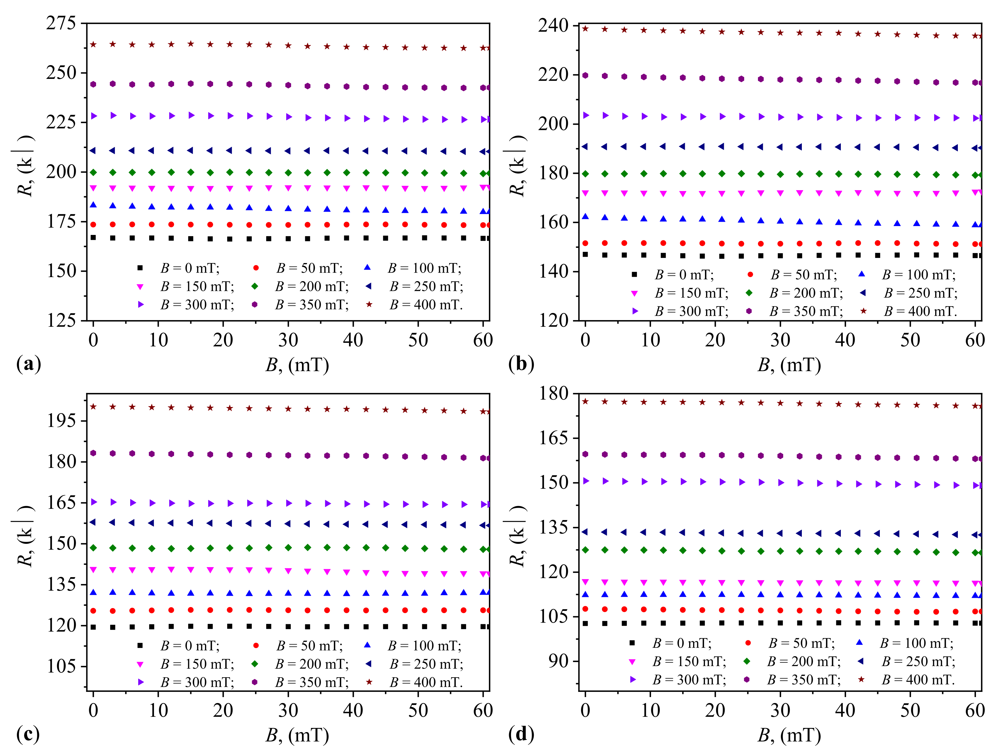
Figure A3 shows that the values of the resistance decrease with the increase in , in accordance with Equation (A20) from Appendix E. However, at the same values of and at times t, it is observed that the values () increase with the increase in B of the magnetic flux density, contrary to Equation (A19) from Appendix E.
This discrepancy is due to the hematite in the composition of the mFe microfibers. It is known that hematite nano-microparticles polarize in the Earth’s magnetic field. By applying an external magnetic field, the hematite nano-microparticles form chains between the magnetite nano-microparticles through magnetic polarization. The length of these chains increases with the increase in B of the magnetic flux density. It is known that hematite nano-microparticles are iron oxide semiconductors with much lower electrical conductivity compared to magnetite nano-microparticles. The resulting effect is an increase in the equivalent electrical resistance of the capacitors CEC with the increase in B of the magnetic flux density, contrary to the effects observed in liquid composites based on carbonyl iron microparticles [24,26,28].
Figure A2.
Variation with time of capacitance, at different values of magnetic flux density. (a) CEC. (b) CEC. (c) CEC. (d) CEC.
Figure A2.
Variation with time of capacitance, at different values of magnetic flux density. (a) CEC. (b) CEC. (c) CEC. (d) CEC.
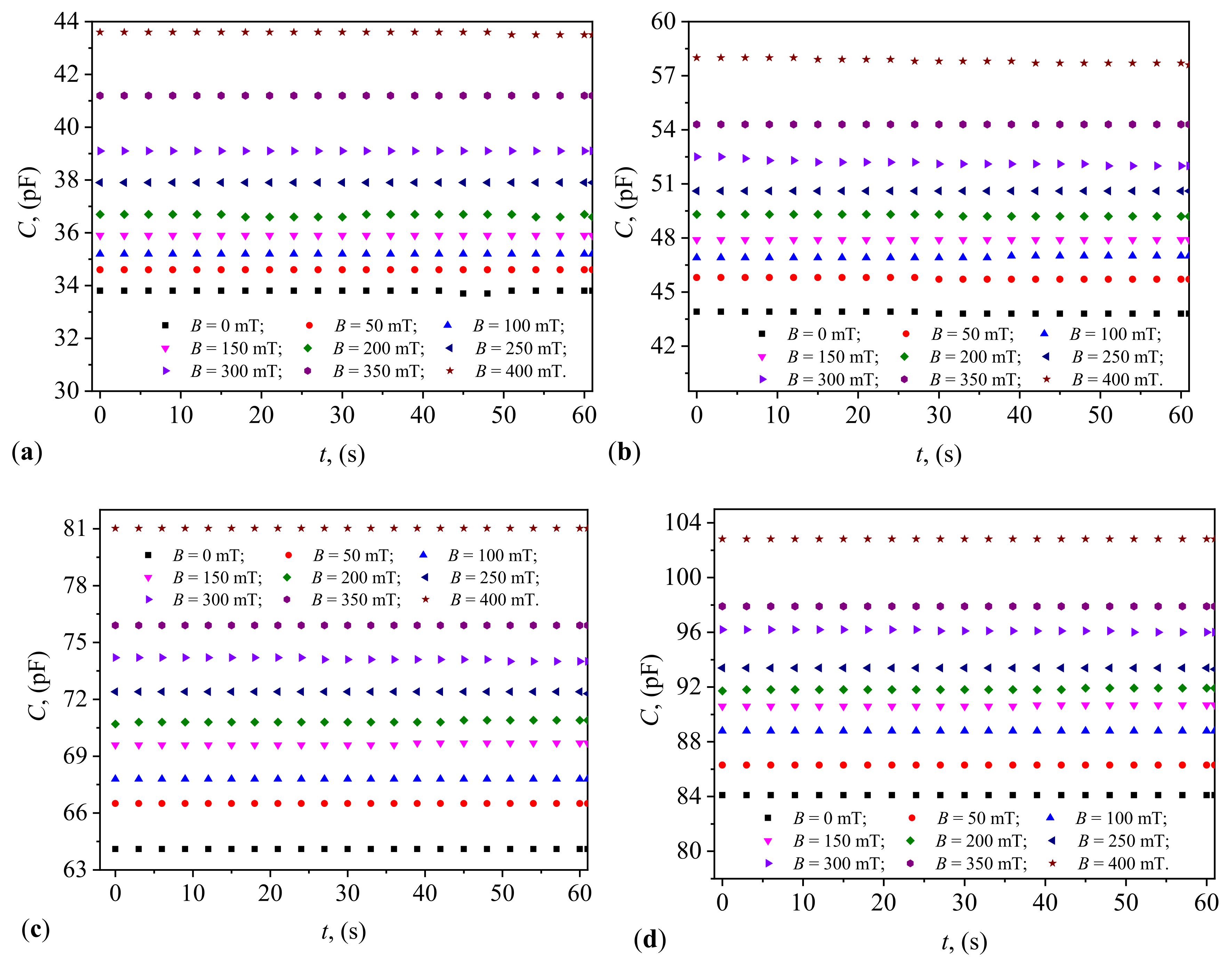
Figure A3.
Variation with time of resistance, at different values of magnetic flux density. (a) CEC. (b) CEC. (c) CEC. (d) CEC.
Figure A3.
Variation with time of resistance, at different values of magnetic flux density. (a) CEC. (b) CEC. (c) CEC. (d) CEC.
Appendix C. Arrangement of Microfibers without and with an External Magnetic Field
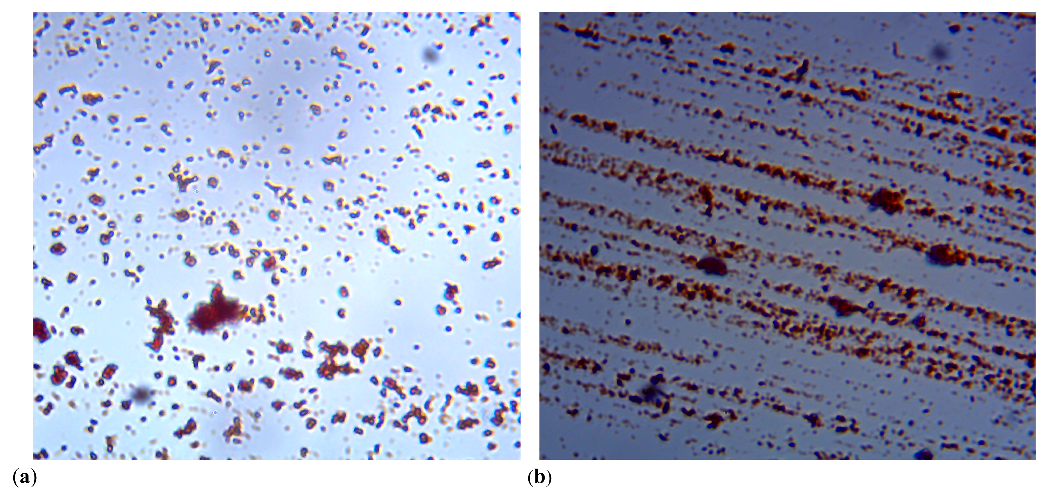
In the absence of any external field, the microfibers form aggregates randomly dispersed within the SO matrix, as shown in Figure A4(a). When an external field is applied, the aggregates are arranged in chain-like structures, as shown in Figure A4(b).
Figure A4.
Microfibers (orange-brown aggregates) in SO (light blue). (a) Without any external field. (b) In the presence of a small magnetic field (about 20 mT).
Figure A4.
Microfibers (orange-brown aggregates) in SO (light blue). (a) Without any external field. (b) In the presence of a small magnetic field (about 20 mT).
Appendix D. Equation of Motion of Microfiber’s Microparticles in a Uiform Magnetic Field
In SO, the microparticles P from the iron oxide microfibers form a composite liquid, denoted as CL. Inside CL, the microparticles P have the same diameter, equal to the average diameter . The microparticles consist of iron oxides in the form of hematite, maghemite, and magnetite.
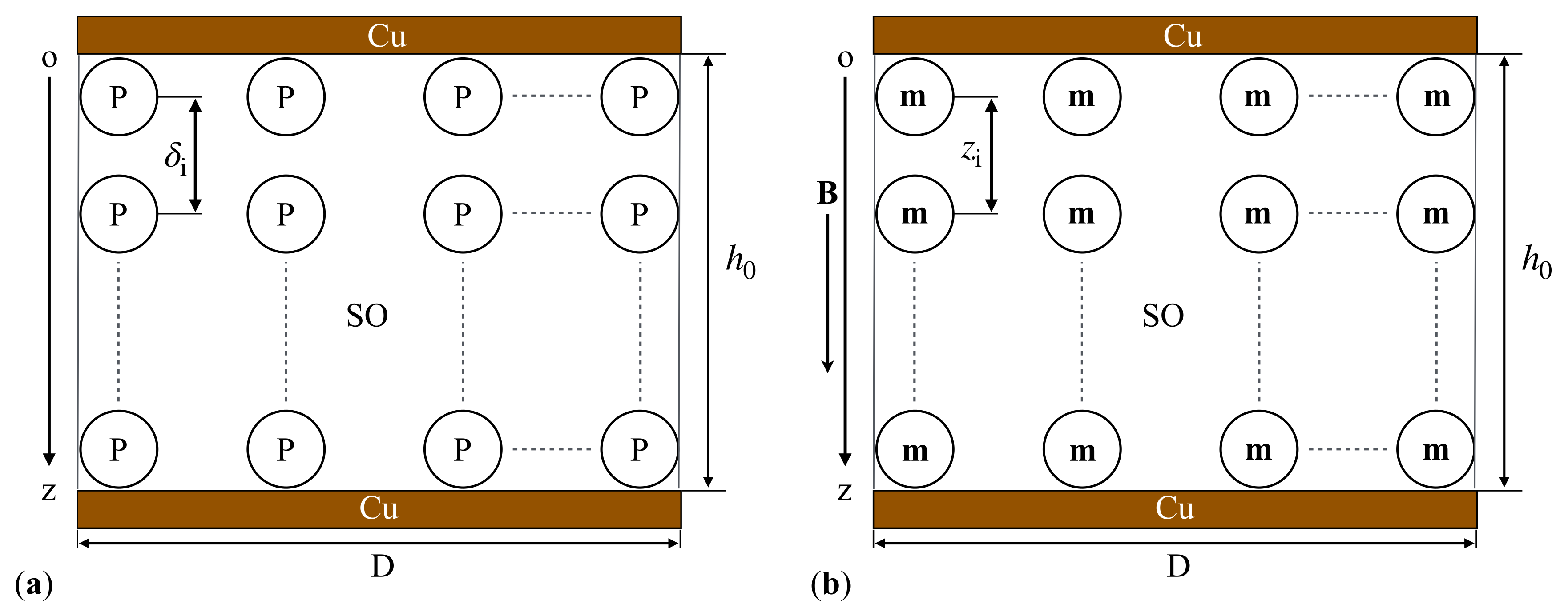
The liquid CL is introduced into a cylinder made of textolite, with bases formed by copper electrodes. This assembly is referred to as a cylindrical electric capacitor, denoted as CEC. At time , the CEC capacitor is introduced in a uniform magnetic field. At this point (see Figure A4a), the microparticles P transform into magnetic dipoles. The magnetic dipoles m are oriented along the direction of the axis, which is identical to the direction of the magnetic flux density vector B. The dipoles m interact with each other, forming aggregates in the shape of columns (Figure A4b). These columns are uniformly distributed in the SO. The projection of the magnetic moment m on the direction of the axis is given by [24,28]:
where is the average diameter, B is the magnetic flux density, and is the magnetic constant of the vacuum. At the initial moment (), the distance () between two identical and neighboring magnetic dipoles m is the same in each column. The distances for the composite liquids in Table (Table 1) are calculated using the expression [24,28]:
where is the average diameter of the dipoles m, and is the volume fraction of the microparticles P in the composite liquids.
Along the axis, there is a magnetic interaction between two neighboring and identical dipoles. The intensity of the dipolar magnetic interaction projected along the axis is given by [24,28]:
where m is the magnetic dipole moment and is the distance between the centers of mass of the magnetic dipoles at a time from the application of B. From Equations (A2) and (A3), we obtain the expression for the intensity of the interaction between two neighboring and identical dipoles in the presence of the magnetic flux density:
The negative sign in Equation (A5) indicates that the microparticles P attract each other.
Figure A5.
Model of a cross-sectional view of the CEC, without (a) and with (b) a magnetic field. P - iron oxide microparticles, SO - silicone oil, Cu - copper plates, D - diameter of CEC, - height of CEC, B and m - magnetic flux density vector, and respectively, dipolar electric moment, and - distances between center of masses of microparticles P within the CL, Oz - coordinate axis.
In the time interval , the distance between the centers of mass of two identical and neighboring dipoles m decreases by an absolute value . From the composite liquid CL, the action of is opposed by a resistance force . The resistance force is the Stokes force, given by:
where is the dynamic viscosity of the CL in the magnetic field at an arbitrary time t.
At an arbitrary moment t, a dynamic equilibrium is established, which mathematically is expressed by the equality of the two forces. Thus, we obtain the equation of motion of the dipoles m in the liquids CL in a magnetic field:
At the moment of application of B (), the distance between the centers of mass of the solid microparticles in the CL is , and at the moment of dynamic equilibrium (), the distance between the same centers of mass is . Using these conditions, we integrate Equation (A7), and in the obtained result, we introduce Equation (A2) to obtain:
Equation (A8) represents the equation of motion of the dipoles m in CL in a magnetic field at an arbitrary moment t. It is observed from Equation (A7) that the motion of the dipoles m in the liquids CL in a magnetic field is uniform. The distance between the centers of mass of the dipoles m, for a fixed value of the diameter and the volume fraction of microparticles, is significantly dependent on the values of B of the magnetic flux density.
Appendix E. Electrical Capacitance and Resistance of CECs
The results obtained in Figures A2 and A3 lead us to conclude that capacitors made with the dielectric liquids CL () have an equivalent electrical circuit consisting of a resistor R connected in parallel with a capacitor C. Using the model from Figure A5, we determine here the analytical expressions for the equivalent electrical resistance and capacitance.
First, we consider that the maximum number, of dipoles m in each chain is estimated by the relation:
where and are the distance between the copper electrodes of the capacitors CEC and the average diameter of the dipoles m.The number of magnetic dipoles m in the liquids CL is estimated by the relation [24,28]:
where is the volume of an average particle. For and , substituted in Equation (A10), we obtain:
Using Equations (A8) and (A10), we obtain the number of columns, , in the volume of the liquids CL as follows:
Each pair of two dipoles in each chain present in the liquids CL forms a microelectric resistor , connected electrically in parallel with a microelectric capacitor . We consider the microresistor to be linear and the microcapacitor to be equivalent to a planar one. Then, the resistance of the microresistors can be approximated by the relation and the capacitance of the microcapacitors by the relation , where and are the electrical conductivity and relative dielectric permittivity of the liquids CL in the magnetic field, is the dielectric permittivity of the vacuum, S is the contact surface area between the dipoles m, and is the distance between the magnetic dipoles at a time . For and the expression of in Equation A7 introduced into the expressions for and , we obtain:
and
The capacitors in the chains of magnetic dipoles are connected in series, and their number is . Then, the capacitance of a chain of capacitors is estimated by the relation:
The capacitors are connected in parallel through the copper foil of the capacitors CEC () in the magnetic field. Then, the equivalent capacitance of the cylindrical capacitors is given by:
where is the initial capacitance of the capacitors CEC.
The value of is calculated using the relation:
The equivalent resistance of a chain of magnetic dipoles, in number , is formed by the sum of the resistances in each chain of magnetic dipoles, and is given by:
The resistances () are connected in parallel through the copper foil of the capacitors CEC in the magnetic field. Then, the equivalent resistance of the capacitors is estimated by the relation:
where are the initial equivalent electrical resistances of the capacitors CEC. The value of is calculated using the relation:
Appendix F. Susceptance and Conductance of CECs
The susceptance and electrical conductance of the capacitors CEC are defined by the following relations:
where is the initial susceptance of the capacitors CEC and f is the frequency of the alternating electric field.
The value of is defined by the expression:
The conductance of the capacitors CEC is defined by the relation:
where is the initial conductance of the capacitors CEC, and is defined by the expression:
References
- Ariyarathna, T.; Kularatna, N.; Gunawardane, K.; Jayananda, D.; Steyn-Ross, D.A. Development of Supercapacitor Technology and Its Potential Impact on New Power Converter Techniques for Renewable Energy. IEEE J. Emerg. Sel. Topics Ind. Electr. 2021, 2, 267–276. [Google Scholar] [CrossRef]
- Subasinghage, K.; Gunawardane, K.; Padmawansa, N.; Kularatna, N.; Moradian, M. Modern Supercapacitors Technologies and Their Applicability in Mature Electrical Engineering Applications. Energies 2022, 15. [Google Scholar] [CrossRef]
- Laadjal, K.; Cardoso, A.J.M. Multilayer Ceramic Capacitors: An Overview of Failure Mechanisms, Perspectives, and Challenges. Electronics 2023, 12. [Google Scholar] [CrossRef]
- Abid, D.; Mjejri, I.; Oueslati, A.; Guionneau, P.; Pechev, S.; Daro, N.; Elaoud, Z. A Nickel-Based Semiconductor Hybrid Material with Significant Dielectric Constant for Electronic Capacitors. ACS Omega 2024, 9, 12743–12752. [Google Scholar] [CrossRef] [PubMed]
- Chaban, V.V.; Andreeva, N.A. Higher hydrogen fractions in dielectric polymers boost self-healing in electrical capacitors. Phys. Chem. Chem. Phys. 2024, 26, 3184–3196. [Google Scholar] [CrossRef] [PubMed]
- Yadlapalli, R.T.; Alla, R.R.; Kandipati, R.; Kotapati, A. Super capacitors for energy storage: Progress, applications and challenges. J. Energy Storage 2022, 49, 104194. [Google Scholar] [CrossRef]
- Torki, J.; Joubert, C.; Sari, A. Electrolytic capacitor: Properties and operation. J. Energy Storage 2023, 58, 106330. [Google Scholar] [CrossRef]
- He, Q.; Sun, K.; Shi, Z.; Liu, Y.; Fan, R. Polymer dielectrics for capacitive energy storage: From theories, materials to industrial capacitors. Mater. Today 2023, 68, 298–333. [Google Scholar] [CrossRef]
- Wang, C.; Ali, L.; Meng, F.Y.; Adhikari, K.K.; Zhou, Z.L.; Wei, Y.C.; Zou, D.Q.; Yu, H. High-Accuracy Complex Permittivity Characterization of Solid Materials Using Parallel Interdigital Capacitor- Based Planar Microwave Sensor. IEEE Sens. J. 2021, 21, 6083–6093. [Google Scholar] [CrossRef]
- Sun, Z.; Wen, X.; Wang, L.; Yu, J.; Qin, X. Capacitor-inspired high-performance and durable moist-electric generator. Energy Environ. Sci. 2022, 15, 4584–4591. [Google Scholar] [CrossRef]
- Ma, Z.; Zhang, Y.; Zhang, K.; Deng, H.; Fu, Q. Recent progress in flexible capacitive sensors: Structures and properties. Nano Mater. Sci. 2023, 5, 265–277. [Google Scholar] [CrossRef]
- Zhou, B.; Dong, Y.; Chi, Q.; Zhang, Y.; Chang, L.; Gong, M.; Huang, J.; Pan, Y.; Wang, X. Fe-based amorphous soft magnetic composites with SiO2 insulation coatings: A study on coatings thickness, microstructure and magnetic properties. Ceram. Int. 2020, 46, 13449–13459. [Google Scholar] [CrossRef]
- Pawar, S.G.; Pradnyakar, N.V.; Modak, J.P. Piezoelectric transducer as a renewable energy source: A review. J. Phys.: Conf. Ser. 2021, 1913, 012042. [Google Scholar] [CrossRef]
- Gemelli, A.; Tambussi, M.; Fusetto, S.; Aprile, A.; Moisello, E.; Bonizzoni, E.; Malcovati, P. Recent Trends in Structures and Interfaces of MEMS Transducers for Audio Applications: A Review. Micromachines 2023, 14. [Google Scholar] [CrossRef]
- Zhang, T.; Sun, H.; Yin, C.; Jung, Y.H.; Min, S.; Zhang, Y.; Zhang, C.; Chen, Q.; Lee, K.J.; Chi, Q. Recent progress in polymer dielectric energy storage: From film fabrication and modification to capacitor performance and application. Progr. Mater. Sci. 2023, 140, 101207. [Google Scholar] [CrossRef]
- Huang, S.; Liu, K.; Zhang, W.; Xie, B.; Dou, Z.; Yan, Z.; Tan, H.; Samart, C.; Kongparakul, S.; Takesue, N.; et al. All-Organic Polymer Dielectric Materials for Advanced Dielectric Capacitors: Theory, Property, Modified Design and Future Prospects. Polym. Rev. 2023, 63, 515–573. [Google Scholar] [CrossRef]
- Adekunle, A.A.; Oparanti, S.O.; Fofana, I. Performance Assessment of Cellulose Paper Impregnated in Nanofluid for Power Transformer Insulation Application: A Review. Energies 2023, 16. [Google Scholar] [CrossRef]
- Khan, S.A.; Tariq, M.; Khan, A.A.; Alamri, B. Effect of Iron/Titania-Based Nanomaterials on the Dielectric Properties of Mineral Oil, Natural and Synthetic Esters as Transformers Insulating Fluid. IEEE Access 2021, 9, 168971–168980. [Google Scholar] [CrossRef]
- Yao, K.; Chen, S.; Rahimabady, M.; Mirshekarloo, M.S.; Yu, S.; Tay, F.E.H.; Sritharan, T.; Lu, L. Nonlinear dielectric thin films for high-power electric storage with energy density comparable with electrochemical supercapacitors. IEEE Trans. Ultrason. Ferroelectr. Freq. 2011, 58, 1968–1974. [Google Scholar] [CrossRef]
- Bird, J. Electrical Circuit Theory and Technology, 6th ed.; Routledge, London, 2017. [CrossRef]
- Huang, J.; Sumpter, Bobby, G.; Meunier, V. A Universal Model for Nanoporous Carbon Supercapacitors Applicable to Diverse Pore Regimes, Carbon Materials, and Electrolytes. Chem. Eur. J. 2008, 14, 6614–6626. [CrossRef] [PubMed]
- Yu, Y.; Li, C.; Wang, H.; Chen, J.; Zhu, X.; Ying, Z.; Song, Y. High-specific-capacitance electrolytic capacitors based on anodic TiO2 nanotube arrays. Electrochim. Acta 2022, 429, 140974. [Google Scholar] [CrossRef]
- Liu, S.; Wei, L.; Wang, H. Review on reliability of supercapacitors in energy storage applications. Appl. Energy 2020, 278, 115436. [Google Scholar] [CrossRef]
- Andrei, O.E.; Bica, I. Some mechanisms concerning the electrical conductivity of magnetorheological suspensions in magnetic field. J. Ind. Eng. Chem. 2009, 15, 573–577. [Google Scholar] [CrossRef]
- Bica, I.; Anitas, E. Magnetic field intensity effect on electrical conductivity of magnetorheological biosuspensions based on honey, turmeric and carbonyl iron. J. Ind. Eng. Chem. 2018, 64, 276–283. [Google Scholar] [CrossRef]
- Bica, I.; Anitas, E. Magnetodielectric effects in membranes based on magnetorheological bio-suspensions. Mater. & Des. 2018, 155, 317–324. [Google Scholar] [CrossRef]
- Bica, I.; Anitas, E.M.; Chirigiu, L. Hybrid Magnetorheological Composites for Electric and Magnetic Field Sensors and Transducers. Nanomaterials 2020, 10. [Google Scholar] [CrossRef] [PubMed]
- Iacobescu, G.E.; Bunoiu, M.; Bica, I.; Sfirloaga, P.; Chirigiu, L.M.E. A Cotton Fabric Composite with Light Mineral Oil and Magnetite Nanoparticles: Effects of a Magnetic Field and Uniform Compressions on Electrical Conductivity. Micromachines 2023, 14. [Google Scholar] [CrossRef]
- Bica, I.; Anitas, E.M.; Choi, H.J.; Sfirloaga, P. Microwave-assisted synthesis and characterization of iron oxide microfibers. J. Mater. Chem. C 2020, 8, 6159–6167. [Google Scholar] [CrossRef]
- Genç, S. Synthesis and Properties of Magnetorheological (MR) fluids. Phd thesis, University of Pittsburg, Pittsburg, 2002. Available online: http://d-scholarship.pitt.edu/8924/1/genc12-20.pdf.
- Baabu, P.R.S.; Kumar, H.K.; Gumpu, M.B.; Babu K, J.; Kulandaisamy, A.J.; Rayappan, J.B.B. Iron Oxide Nanoparticles: A Review on the Province of Its Compounds, Properties and Biological Applications. Materials 2023, 16. [Google Scholar] [CrossRef] [PubMed]
- Meijer, J.M.; Rossi, L. Preparation, properties, and applications of magnetic hematite microparticles. Soft Matter 2021, 17, 2354–2368. [Google Scholar] [CrossRef]
- Malasi, A.; Taz, H.; Farah, A.; Patel, M.; Lawrie, B.; Pooser, R.; Baddorf, A.; Duscher, G.; Kalyanaraman, R. Novel Iron-based ternary amorphous oxide semiconductor with very high transparency, electronic conductivity and mobility. Sci. Rep. 2015, 5, 18157. [Google Scholar] [CrossRef] [PubMed]
- Pal, R. Recent Progress in the Viscosity Modeling of Concentrated Suspensions of Unimodal Hard Spheres. ChemEngineering 2023, 7, 70. [Google Scholar] [CrossRef]
- Batchelor, G.K. The effect of Brownian motion on the bulk stress in a suspension of spherical particles. J. Fluid Mech. 1977, 83, 97–117. [Google Scholar] [CrossRef]
- Felicia, L.J.; John, R.; Philip, J. Rheological Properties of Magnetorheological Fluid with Silica Nanoparticles StabilizersA Comparison with Ferrofluid. J. Nanofluids 2013, 2, 75–84. [Google Scholar] [CrossRef]
- Chauhan, Vinod.; Kumar, Ashwani.; Sham, Radhey. Magnetorheological fluids: A comprehensive review. Manufacturing Rev. 2024, 11, 6. [CrossRef]
- Bica, I.; Anitas, E.M.; Averis, L.M.E.; Kwon, S.H.; Choi, H.J. Magnetostrictive and viscoelastic characteristics of polyurethane-based magnetorheological elastomer. J. Ind. Eng. Chem. 2019, 73, 128–133. [Google Scholar] [CrossRef]
- Wu, M.; Xiong, Y.; Jia, Y.; Niu, H.; Qi, H.; Ye, J.; Chen, Q. Magnetic field-assisted hydrothermal growth of chain-like nanostructure of magnetite. Chem. Phys. Lett. 2005, 401, 374–379. [Google Scholar] [CrossRef]
- Zhang, X.; Lu, W.; Zhou, G.; Li, Q. Understanding the Mechanical and Conductive Properties of Carbon Nanotube Fibers for Smart Electronics. Adv. Mater. 2020, 32, 1902028. [Google Scholar] [CrossRef] [PubMed]
Figure 1.
(a) PCB. 1 - copper foil. (b) Cylinder. 1 - copper foil, 2 - dielectric ring.
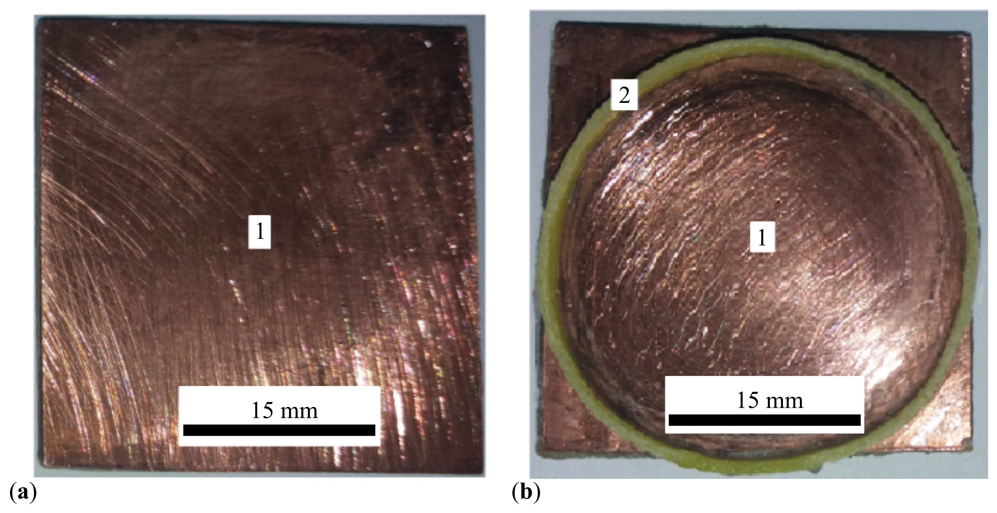
Figure 2.
(a) Cylinder with CL. 1 - copper foil, 3 - CL, 4 - electrical contact. (b) Cylinder with CL and with textolite plate on top. 2 - dielectric ring, 5 - textolite plates. (c) CEC. 6 - adhesive medical tape. 7 - terminals for electrical contact.
Figure 2.
(a) Cylinder with CL. 1 - copper foil, 3 - CL, 4 - electrical contact. (b) Cylinder with CL and with textolite plate on top. 2 - dielectric ring, 5 - textolite plates. (c) CEC. 6 - adhesive medical tape. 7 - terminals for electrical contact.
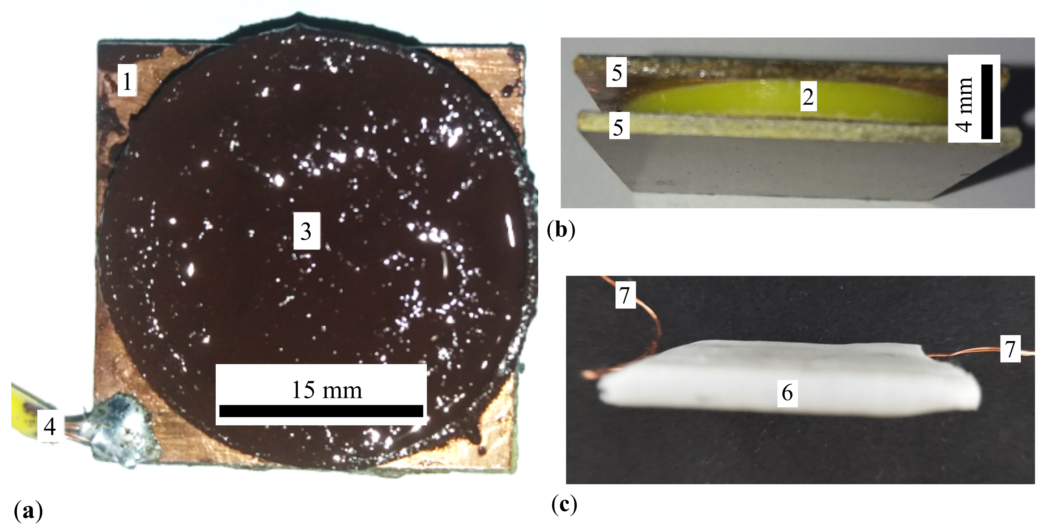
Figure 3.
Schematic view of the experimental setup. 1 - magnetic yoke, 2 - coil, DCS - direct current source, Br - RLC bridge, Gs - gaussmeter, h - Hall probe, CU - computing unit, CEC - electrical capacitor based on CL, B - magnetic flux density vector.
Figure 3.
Schematic view of the experimental setup. 1 - magnetic yoke, 2 - coil, DCS - direct current source, Br - RLC bridge, Gs - gaussmeter, h - Hall probe, CU - computing unit, CEC - electrical capacitor based on CL, B - magnetic flux density vector.
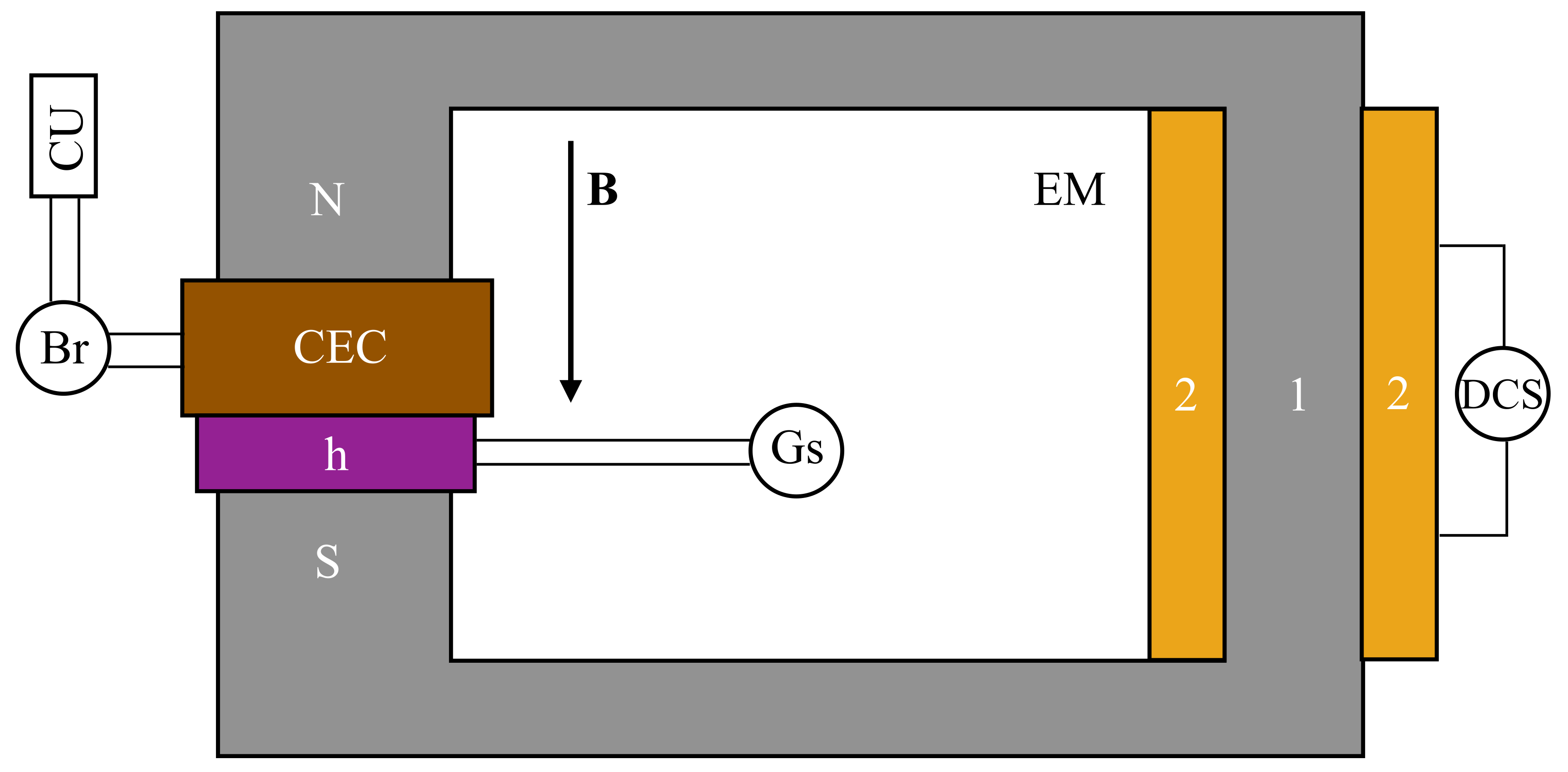
Figure 4.
Variation with time of the susceptance of CECs, at different values of the magnetic flux density. (a) CEC. (b) CEC. (c) CEC. (d) CEC.
Figure 4.
Variation with time of the susceptance of CECs, at different values of the magnetic flux density. (a) CEC. (b) CEC. (c) CEC. (d) CEC.
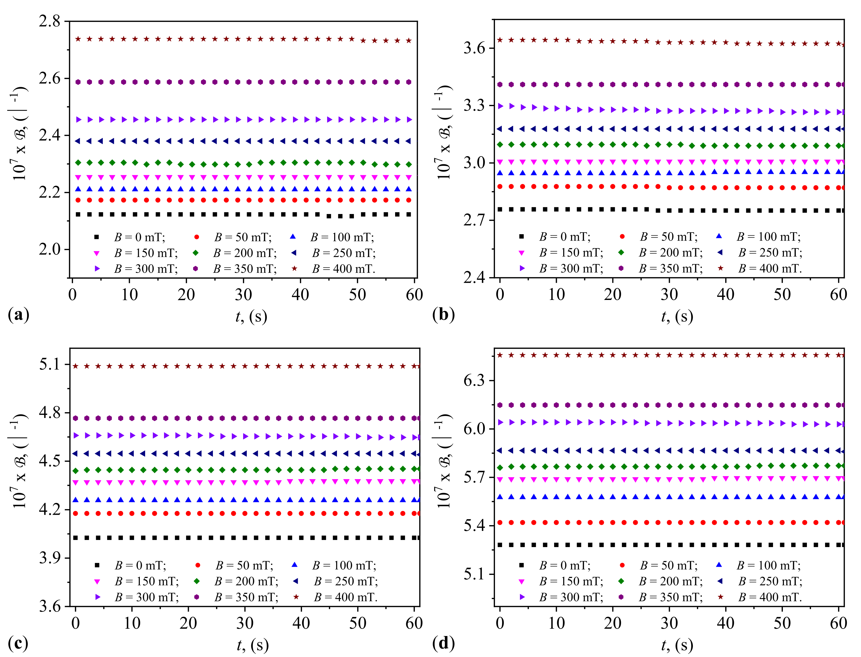
Figure 5.
Variation with time of the conductance of CECs, at different values of the magnetic flux density. (a) CEC. (b) CEC. (c) CEC. (d) CEC.
Figure 5.
Variation with time of the conductance of CECs, at different values of the magnetic flux density. (a) CEC. (b) CEC. (c) CEC. (d) CEC.
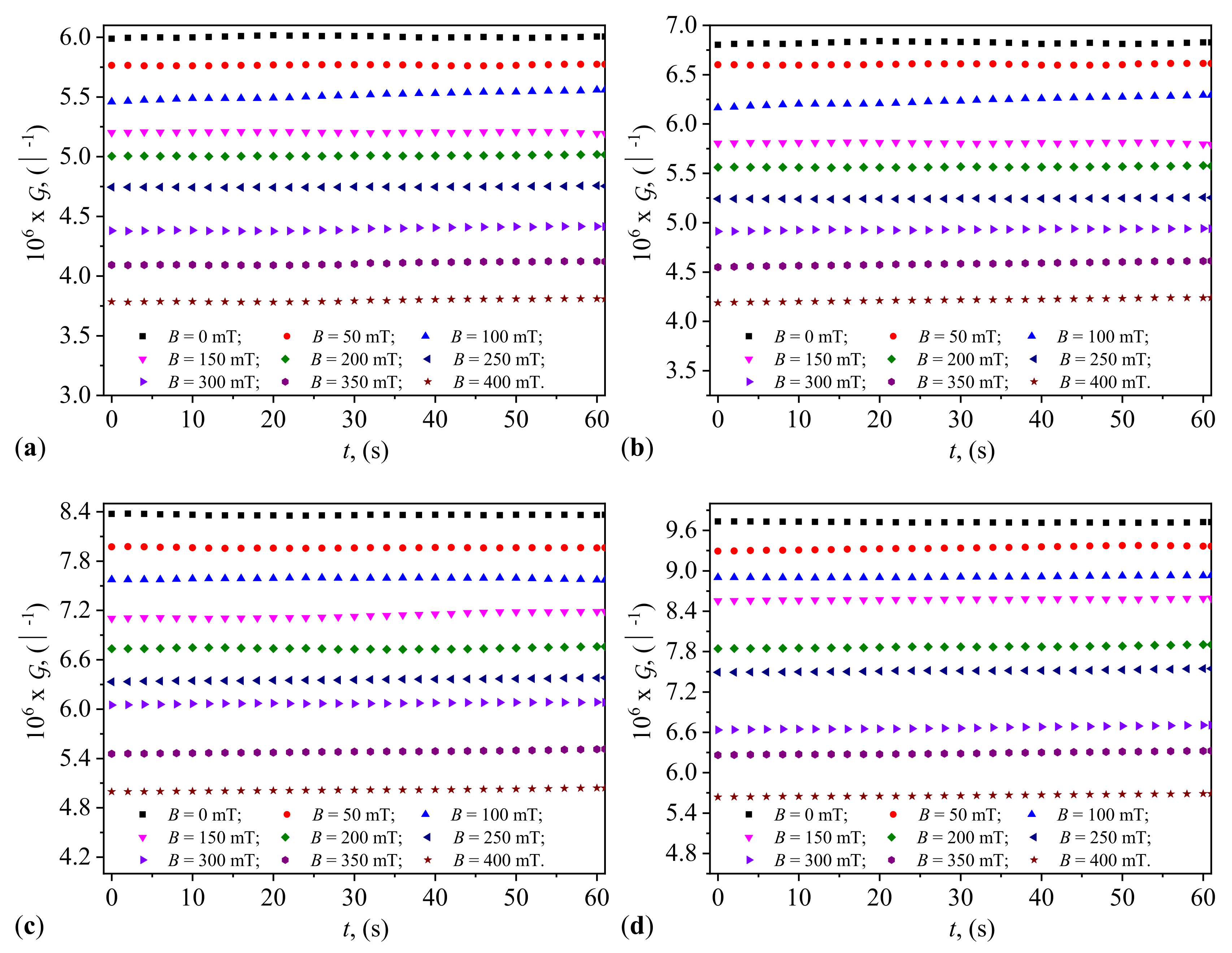
Figure 6.
Variation with magnetic flux density of the susceptance (a) and conductance (b) for CECs.
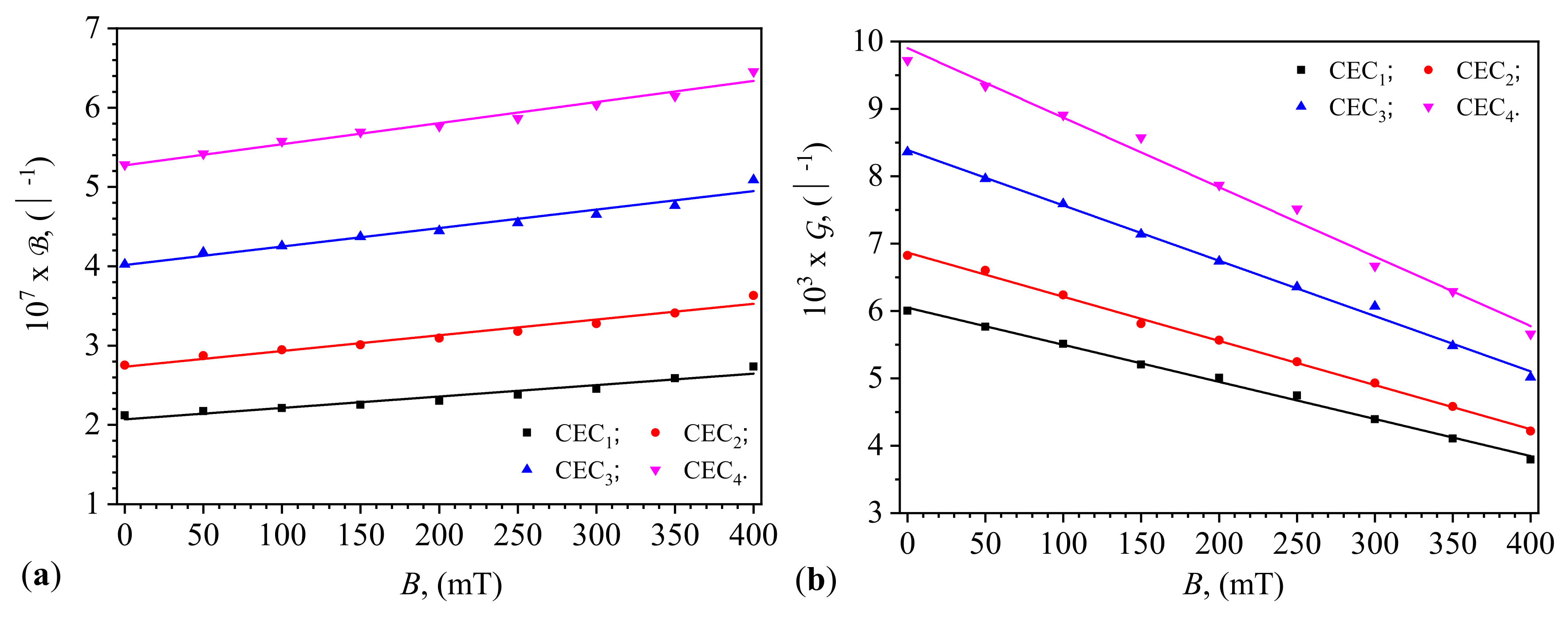
Figure 7.
Variation of the viscosity with magnetic flux density (a), and with magnetic flux density and conductance (b) for CECs.
Figure 7.
Variation of the viscosity with magnetic flux density (a), and with magnetic flux density and conductance (b) for CECs.
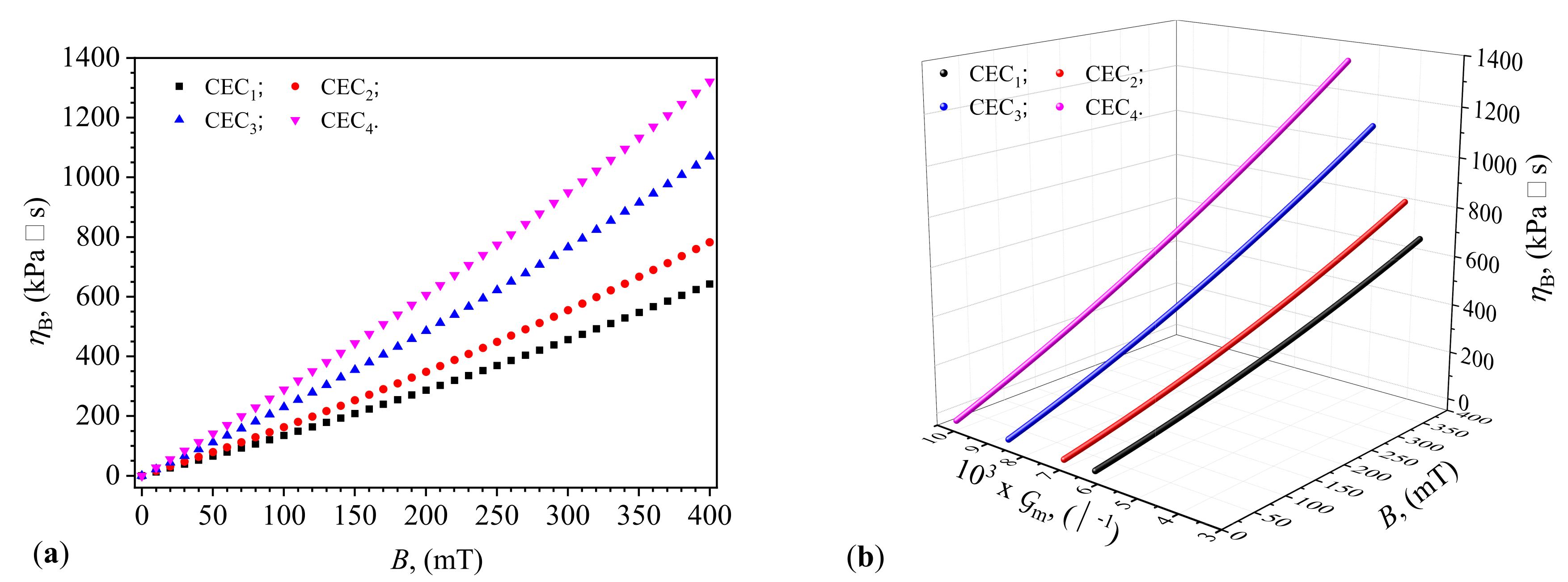
Figure 8.
(a) Variation of average conductance with average susceptance for CECs. (b) Variation of time constant with magnetic flux density for CECs.
Figure 8.
(a) Variation of average conductance with average susceptance for CECs. (b) Variation of time constant with magnetic flux density for CECs.


Table 1.
The composition of CLs and their saturation magnetization (). and are the volume, and respectively mass fractions of mFe.
Table 1.
The composition of CLs and their saturation magnetization (). and are the volume, and respectively mass fractions of mFe.
| mFe, (cm) | mFe, (g) | SO, (cm) | SO, (g) | , (vol.%) | , (wt.%) | , (A·m/kg) | |
|---|---|---|---|---|---|---|---|
| CL | 0.20 | 0.575 | 1.80 | 1.75 | 10 | 24.8 | 2.27 |
| CL | 0.40 | 1.150 | 1.40 | 1.55 | 20 | 42.6 | 9.08 |
| CL | 0.60 | 1.725 | 1.60 | 1.36 | 30 | 56.0 | 13.62 |
| CL | 0.80 | 2.300 | 1.20 | 1.16 | 40 | 66.4 | 21.16 |
| , () | , (/mT) | , () | , (/mT) | |
|---|---|---|---|---|
| CEC | 2.070 ± 0.034 | 0.001 ± 1.409 · 10 | 6.049 ± 0.030 | 0.006 ± 1.188 · 10 |
| CEC | 2.733 ± 0.034 | 0.002 ± 1.412 · 10 | 6.867 ± 0.030 | 0.007 ± 1.166 · 10 |
| CEC | 4.016 ± 0.043 | 0.002 ± 1.785 · 10 | 6.388 ± 0.042 | 0.008 ± 1.757 · 10 |
| CEC | 5.273 ± 0.039 | 0.003 ± 1.617 · 10 | 9.901 ± 0.092 | 0.010 ± 3.849 · 10 |
Disclaimer/Publisher’s Note: The statements, opinions and data contained in all publications are solely those of the individual author(s) and contributor(s) and not of MDPI and/or the editor(s). MDPI and/or the editor(s) disclaim responsibility for any injury to people or property resulting from any ideas, methods, instructions or products referred to in the content. |
© 2024 by the authors. Licensee MDPI, Basel, Switzerland. This article is an open access article distributed under the terms and conditions of the Creative Commons Attribution (CC BY) license (http://creativecommons.org/licenses/by/4.0/).
Copyright: This open access article is published under a Creative Commons CC BY 4.0 license, which permit the free download, distribution, and reuse, provided that the author and preprint are cited in any reuse.


