Submitted:
18 June 2024
Posted:
19 June 2024
You are already at the latest version
Abstract
Underwater imaging presents unique challenges, notably color distortions and reduced contrast due to light attenuation and scattering. Most underwater image enhancement methods, first use linear transformations for color compensation and then enhance the image. We observed that linear transformation for color compensation is not suitable for certain images. For such images, a non-linear mapping is a better choice. Our paper introduces a unique underwater image restoration approach leveraging a streamlined convolutional neural network (CNN) for dynamic weight learning for linear and non-linear mapping. In the first phase, a classifier is applied that classifies the input images into Type-I or Type-II. In the second phase, depending on the classification, the Deep Line Model (DLM) for Type-I images or the Deep Curve Model (DCM) for Type-II images. For mapping an input image to an output image, DML creatively combines color compensation and contrast adjustment in a single step and uses deep lines for transformation, whereas DCM employs higher-order curves. Both models utilize lightweight neural networks that learn per-pixel dynamic weights based on the input image’s characteristics. Comprehensive evaluations on benchmark datasets using metrics like peak signal-to-noise ratio(PSNR) and root mean squares error (RMSE) affirm our method’s effectiveness in accurately restoring underwater images, outperforming existing techniques.
Keywords:
underwater images
; underwater image restoration
; underwater image enhancement
; color restoration
; lightweight network
; deep learning
1. Introduction
Underwater imaging plays an important role in ocean observation and marine engineering applications. However, underwater images suffer from several artifacts. While capturing underwater images, a considerable portion of the light is absorbed during its propagation in the water, resulting in color distortion [1]. Moreover, backward-forward light scattering severely affects the contrast and details of images, which further deteriorates the performance of underwater industrial applications [2]. Therefore, Underwater Image Enhancement – addressing color restoration, enhancing contrast, and improving details – is an essential task in marine engineering and observation applications.
In the literature, many methods have been proposed for improving underwater image quality. These methods can be broadly categorized into prior-based, imaging-based, and machine-deep learning-based techniques [3]. Prior-based methods utilize the underwater image formation model (IFM) and draw priors from the degraded images. Initially, a transmission map (TM) is derived from priors such as the dark-channel prior (DCP) [4], red-channel prior (RCP) [5], medium-channel prior (MDP) [6], and haze-line prior (NLD) [7]. Subsequently, the image is restored using the IFM, equipped with the TM and atmospheric light. In [8], a red channel prior (RCP)-guided variational framework is introduced to enhance the TM, and the image is restored utilizing the IFM. Generally, these methods heavily depend on hand-crafted priors and excel in dehazing outdoor images. However, their performance is less than satisfactory for underwater images, and they struggle to correctly manage color shifts.
Imaging-based methods, in contrast to the prior ones, do not utilize the IFM. Instead, they rely on foundational image enhancement techniques such as contrast enhancement, histogram equalization, image fusion, and depth estimation. Peng et al. [2] proposed a depth estimation technique for underwater scenes that relies on image blurriness and light absorption. This depth information is fed into the IFM to restore and enhance the underwater visuals. In another study by Ancuti et al. [9], a combined approach of color compensation and white balancing is applied to the original degraded image to restore its clarity. Zhang et al. [10] introduced a strategy guided by the minimum color loss principle and maximum attenuation map to adjust for color shifts. In another recent work by Zhang et al. [11], a Retinex-inspired color correction mechanism is employed to eliminate color cast. The research further incorporates both local and global contrast-enhanced versions of the image to refine the color output. Although these approaches significantly improve the color and contrast of underwater images, they often overlook the specificities of underwater imaging models. This oversight can result in over-enhanced or over-saturated final images.
On the other hand, deep learning methods are mainly divided into ASM-based and non-ASM-based techniques. ASM-based methods use the Atmospheric Scattering Model to clear up hazy images. For instance, DehazeNet [12] by Cai et al. applies a deep architectural approach to estimate transmission maps, generating clear images. Similarly, MSCNN [13] by Ren et al. uses a multi-scale network to learn the mapping between hazy images and their corresponding transmission maps. AOD-Net [14] by Li et al. directly creates clear images with a lightweight CNN, and DCPDN [15] by Zhang et al. leverages an innovative network architecture, focusing on multi-level pyramid pooling to optimize dehazing performance. In contrast, non-ASM-based methods rely on various network designs to transform hazy images directly into clear ones through various structures like the encoder-decoder, GAN-based, attention-based, knowledge transfer, and transformer-based networks. Encoder-decoder structures like the Gated Fusion Network (GFN) by Ren et al. [16] and Gated Context Aggregation Network (GCANet) by Chen et al. [17] utilize multiple inputs and dilated convolutions to effectively reduce halo effects and enhance feature extraction. GAN-based networks such as Cycle-Dehaze by Engin et al. [18] and BPPNet by Singh et al. [19] offer unpaired training processes and are capable of learning multiple complexities, thereby yielding high-quality dehazing results even with minimal training datasets. Attention-based networks like GridDehazeNet by Liu et al. [20] and FFA-Net by Qin et al. [21] implement adaptive and attention-based techniques, providing more flexibility and efficiently dealing with non-homogeneous haze. Knowledge transfer methods like KTDN by Wu et al. [22] leverage teacher-student networks, enhancing performance in non-homogeneous haze conditions by transferring the robust knowledge acquired by the teacher network. Lastly, transformer-based networks like DehazeFormer by Song et al. [23] make significant modifications in traditional structures and employ innovative techniques like SoftReLU and RescaleNorm, presenting better performance in dehazing tasks with efficient computational cost and parameter utilization.
In this study, we propose a method for underwater image restoration that employs linear or non-linear mapping depending on the type of the input image. First, an input image is classified as Type-I or Type-II. Then, the Type-I image is enhanced using the Deep Line Model (DLM), while the Deep Curve Model (DCM) is employed for the Type-II image. The DLM effectively integrates color compensation and contrast adjustment in a unified process, utilizing deep lines for transformation, whereas the DCM is focused on applying higher-order curves for image enhancement. Both models utilize lightweight neural networks that learn per-pixel dynamic weights based on the input image’s characteristics. The efficacy of the proposed method is measured by conducting experiments on benchmark datasets and using quantitative metrics like PSNR and RMSE. The comparative analysis affirms our method’s effectiveness in accurately restoring underwater images, outperforming existing techniques.
2. Motivation
Let represent a degraded underwater color image, where denotes the coordinates of the image pixels and signifies the red, green, and blue color channels, respectively. The color components of the image can thus be denoted as . In underwater imaging, differential color attenuation across wavelengths frequently leads to compromised visual fidelity, predominantly impacting the red channel while leaving the green comparatively unaltered [24]. Conventional restoration techniques typically adopt a sequential approach: initial color correction to balance channel disparities, followed by linear enhancement methods such as contrast stretching to mitigate the attenuation effects.
In literature, many methods use the mean values from each channel for color compensation [9,24,25,26,27]. This approach is grounded in the Gray World assumption, which suggests that all channels should exhibit equal mean intensities in an undistorted image [25], leading to a straightforward approach for color compensation:
where , , and denote the mean values of the degraded color components of the underwater image .
Although additive adjustments can compensate for color distortions in red and blue channels, our study reveals that this compensation may worsen the color composition in many cases, leading to inferior quality in restored images. As demonstrated in Figure 1, two distinct outcomes are observed: Type-I images benefit from color correction, with spectral intensities approaching the ground truth, enhancing visual quality. Conversely, Type-II images experience worsened color discrepancies, resulting in suboptimal restoration. This necessitates a dual restoration approach. Our method uses a classifier to categorize images, followed by the application of the DLM for Type-I and the DCM for Type-II. This strategy ensures precise, adaptive restoration aligned with the specific requirements of each image category.
3. Proposed Method
The proposed methodology restores images through a two-phase process. Initially, an image classifier categorizes each image as either Type-I or Type-II. Subsequently, Type-I images are processed using the Deep Line Model (DLM), while Type-II images undergo enhancement through the Deep Curve Model (DCM). The complete framework depicted in Figure 2 showcases the complete process, from initial classification to the final output, highlighting the effectiveness and adaptability of both DLM and DCM in underwater image restoration.
3.1. Image Classifier
Based on the observations in images’ profile intensity and metrics, images have been categorized into two distinct types. Type-I images are those that retain or improve in quality following linear transformation for color compensation, while Type-II images are characterized by a decline in quality after the same transformation. Following to this classification, we applied linear transformations and computed metrics such as RMSE and PSNR and labelled the images accordingly. For the classification task, DenseNet121 [26] is employed to analyze the intrinsic properties of an input image and to guide it towards the most appropriate restoration pathway—DLM for Type-I and DCM for Type-II images—thereby enhancing feature extraction and image restoration. The subsequent sections delve into the detailed frameworks of each model.
3.2. Deep Line Model
Mostly, underwater image enhancement methods are executed in two linear operations. Initially, a color-corrected image is obtained by compensating the channels through additive adjustment factors [9,27]. The generalized form of this operation is as follows:
where represents the additive adjustment factors for each channel . In the second step, the restored image is obtained by improving contrast. It is achieved by applying another linear operation that stretches the pixel values of the color-corrected image.
where, , are constants utilized to represent weights for each channel that are mostly applied globally.
Instead of performing two separate linear operations and using global weights, we suggest a deep line model that combines two steps and uses per-pixel weights. The proposed model is expressed as;
where, , are weight matrices and color compensation factor for each channel . The color compensation factors are computed by using the mean guided compensations [24] through the following expressions.
where, , , and denote the mean values of degraded color components of underwater image .
Now, the computational challenge exist in in the derivation of dynamic weight matrices. To overcome this, we employ a lightweight deep neural network, as illustrated in Figure 2b. The network’s architecture encompasses seven convolutional layers; the first six are equipped with 16 filters each, kernel and utilizing ReLU activation functions, while the seventh layer adopts a Tanh activation to produce the required weight matrices. This setup is specifically designed to facilitate localized adjustments, empowering the deep line model delineated in Equation (4) to competently address the complex characteristics of underwater images and effectuate precise, adaptive enhancements. Figure 2c exemplifies this capability, depicting the generic behavior of deep lines with varying random parameters , spanning a range from -1 to 1. Our model is not only effective but also efficient, comprising a mere 18,390 trainable parameters and requiring only 54.07 MB of memory, rendering it an optimal solution for resource-constrained systems.
3.3. Deep Curve Model
The images that are not restored through linear operations require non-linear transformations. Inspired by the work [28] for low light image enhancement, we propose a deep curve model for underwater image restoration. A second-order polynomial is a simple non-linear mapping between an input image and the output image which is also differential.
where are pixel-wise coefficients for each channel . By setting , the non-linear mapping can be simplified and re-written as
where are the weight matrices for the non-linear mapping (curves) for each channel . It means that the curves are applied separately to each of the three RGB channels allowing for better restoration by preserving the inherent color and by reducing the risk of over-saturation. Further, the image is restored by applying mapping inside the network, so it should be differentiable for forward and back-word passes. While the second-order curves can provide satisfactory restoration results, however, they can further be improved by applying higher-order curves. One simple way to achieve higher-order mapping is to apply second-order mapping iterative fashion. The iterative version of the deep curve model can be expressed as;
where n indicates the iteration number and are the weight matrices for the iteration. For , is computed through (6). Further, for n iterations, weight matrices are required. In this work, we have set the eight i.e., so dynamic weight matrices are to learn. Now, the problem is how to compute dynamic weight matrices.
To learn the weight matrices (curve parameter maps), we adopted a technique similar to that used in the deep line model discussed in the previous section. A lightweight deep neural network, as shown in Figure 2e, is employed to compute these dynamic weight matrices. The network takes the input image and learns a set of pixel-wise curve parameter maps corresponding to higher-order curves. The behavior of such curves is illustrated in Figure 2f, for instance, , with and set to -1 and the number of iterations n equal to 3, showcasing the advanced adjustment capabilities with these curves. The network’s architecture comprises seven convolutional layers, with the first six layers each containing 32 kernels of size with a stride of 1, followed by a ReLU activation function to introduce non-linearity into the model. The final layer consists of 24 convolutional kernels of the same size and stride but employs a Tanh activation function, ensuring that the output values are constrained within the range of -1 to 1. This layer produces a total of 24 curve parameter maps (dynamic weight matrices) across eight iterations, with each iteration providing three curve parameter maps for each channel .
4. Results and Discussion
4.1. Implementation Details
In this study, we utilized two primary datasets: EUVP [29] and UIEBD [30]. Both datasets comprise subsets containing paired and unpaired images. We aggregated paired images from subsets of EUVP, including underwater_dark, underwater_scenes, and underwater_imagenet, resulting in a combined total of images. These images were used for both training and testing within our proposed method. Similarly, from the UIEBD dataset, we selected 890 images from the raw-890 subset for the same purpose. For performance evaluation, we used the test_samples subsets from both EUVP and UIEBD, which consist of 515 and 240 images respectively.
In our implementation, we constructed the framework using PyTorch and executed on an NVIDIA GeForce RTX3090 GPU. The proposed method integrates three core models: (1) DenseNet121, which differentiates between Type-I and Type-II images. It utilizes a learning rate of and a batch size of 2 across both datasets; (2) DLM targets the enhancement of Type-I images, with configuration settings such as a batch size of 64 and 80 epochs for EUVP, and a batch size of 2 and 200 epochs for UIEBD; (3) DCM focuses on the restoration of Type-II images. This model adopts optimizer configurations similar to the DLM but with a specific batch size of 2 and 100 epochs for EUVP and solely 200 epochs for UIEBD. Throughout their training phases, both the DLM and DCM models employ the RMSE (L2) as loss function. Using the assembled dataset, classifier was trained to categorize the images into two types: Type-I and Type-II. This classification was carried out on images from EUVP and 890 images from UIEBD. As a result, 758 images from EUVP and 240 images from UIEBD were identified as Type-II, while the remaining images were designated as Type-I. The DLM was then trained on Type-I images from EUVP and 500 images from UIEBD. In contrast, the DCM was trained using 758 Type-II images from EUVP and 140 Type-II images from UIEBD. All models utilized the Adam optimizer to ensure efficient convergence. For both training and evaluation, we processed images with dimensions . Importantly, our settings incorporated gradient clipping, normalized to , to prevent gradient explosions, along with a weight decay of to provide regularization.
4.2. Analysis
The proposed method was tested using 515 images from the EUVP dataset and 240 images from the UIEBD dataset. The proposed classifier designated 486 to Type-I and 29 images to Type-II out of 515 images from the EUVP dataset, setting them up as the testing sets for the DLM and DCM, respectively. Similarly, from the UIEBD dataset, test images classified 213 images in Type-I and 27 images in Type-II. All datasets were provided to each of the proposed DLM and DCM for the restoration. RMSE and PSNR metrics were computed for each image in the datasets and the average of the PSNR and RMSE are shown in Table 1. As DLM is designed for refining Type-I images and DCM is developed for the restoration of Type-II images. From the table, it can be observed that when models are applied on Type-I and Type-II images respectively, improved PSNR and RMSE measures are obtained. Whereas, declined or marginally improved metrics are obtained when models are applied on Type-II and Type-I images respectively. Hence, DLM and DCM are effective for the restoration of Type-I and Type-II images respectively.
In addition, for qualitative analysis of DLM and DCM, we selected two images from each Type, and their restored versions are shown in Figure 3. From the analysis of the figure, it is evident that the DLM performs better for Type-I images in both datasets, yielding restored images that are closer to the ground truth (GT). However, when the DCM is applied to Type-I images, although certain areas appear clearer, there is a tendency for colors to become denser. For instance, the blue color intensifies, resulting in a more bluish appearance of the image. Conversely, Type-II images restored using DCM for both datasets exhibit a cleaner look and are more closely aligned with the GT, whereas DLM shows suboptimal performance, either causing color distortion or producing blurry images.
In our detailed examination of the Deep Curve Model (DCM) performance, we observed a consistent enhancement in the restoration quality with increasing iterations. Utilizing two representative images from the UIEBD dataset, as illustrated in Figure 4, we record the progression of quality improvements. For instance, as shown in Figure 4b, the restoration quality at the fourth iteration (I4) manifests a considerable enhancement from the input, evidenced by the RMSE/PSNR values of 0.09/20.95. This trend of enhancement persists through iterations I4 and I6, as highlighted by the corresponding RMSE/PSNR figures, which signify improved clarity and overall quality of the dehazed images. The peak of visual clarity is achieved at iteration I8, registering the lowest RMSE of 0.06 and the highest PSNR of 24.66 for the top image, with the bottom image exhibiting similarly positive metrics. Notably, limiting the model to merely one or two iterations does not invariably lead to inferior dehazing outcomes; in some cases, image quality may remain stable or even slightly enhance, suggesting that the optimal number of iterations for image enhancement is variable. The correlation between the iteration count and the quality of dehazing is evident, with higher iterations yielding superior visual and quantitative results.
4.3. Comparative Analysis
In order to rigorously assess the efficacy of our proposed approach, we contrasted it against leading-edge methods in the domain. This encompasses non-learning techniques such as NLD [7], RLP [31], MMLE [10], and UNTV [8], as well as learning-driven paradigms including ACT [32], FGAN [33], DNet [12], AOD [14], and SCNet [34]. First, input images are restored through the above-mentioned methods and the proposed method, and then restoration accuracy is compared by utilizing the widely accepted quantitative metrics, Root Mean Square Error (RMSE) and Peak Signal-to-Noise Ratio (PSNR). A Lower value for RMSE and a higher value for PSNR indicates better results. Table presents the quantitative results for test samples across both datasets. The performance of the proposed networks for the EUVP dataset is denoted as “Ours”. Focusing on the EUVP dataset, a quick examination of Table 1 reveals that DLM exhibits superior performance in Type-I images, registering a RMSE of 0.08 and a PSNR of 22.30dB, which outperforms state-of-the-art (SOTA) methods. Similarly, for Type-II images, DCM surpasses competing methods by achieving 0.06 RMSE and 25.00dB PSNR. Notably, when contrasted with SCNet and ACT — the models boasting the second-best performance for Type-I and Type-II images respectively — DLM excels with a differential of 0.02 in RMSE and 2.3dB in PSNR, whereas DCM showcases a marked improvement with 0.87 RMSE and 4.4dB PSNR. Transitioning to the UIEBD dataset, SCNet leads in performance for Type-I images, registering 0.07 RMSE and 23.60dB PSNR. This is contrasted with DLM, which holds the position for the second-best performance, achieving 0.11 RMSE and 20.10dB PSNR. Conversely, for Type-II images, DCM stands out by attaining 0.08 RMSE and 22.20dB PSNR. When compared with SCNet — the runner-up in performance — our DCM establishes a superior benchmark with a difference of 0.02 in RMSE and an elevation of 1.5dB in PSNR.

Table 2.
Comparison of Average RMSE and PSNR for Non-Learning & Learning-Based Methods on EUVP and UIEBD Test Images. The best results are in bold and the second best results are with underline.
Table 2.
Comparison of Average RMSE and PSNR for Non-Learning & Learning-Based Methods on EUVP and UIEBD Test Images. The best results are in bold and the second best results are with underline.
| Non-learning-based Methods | Learning-based Methods | |||||||||||
| Dataset | Type | Input | NLD | RLP | MMLE | UNTV | ACT | D-Net | AOD | F-GAN | SCNet | Ours |
| EUVP | Type-I | 0.11/20.00 | 0.15/17.00 | 0.15/17.30 | 0.18/15.30 | 0.14/17.40 | 0.84/17.50 | 0.12/19.10 | 0.78/15.10 | 0.73/13.70 | 0.10/20.00 | 0.08/22.30 |
| Type-II | 0.08/22.00 | 0.12/18.40 | 0.15/16.90 | 0.17/15.60 | 0.11/19.20 | 0.93/20.60 | 0.10/20.10 | 0.87/13.30 | 0.84/15.50 | 0.11/19.70 | 0.06/25.00 | |
| UIEBD | Type-I | 0.15/17.60 | 0.18/15.30 | 0.14/17.50 | 0.21/14.30 | 0.16/16.20 | 0.81/15.50 | 0.17/15.90 | 0.75/15.10 | 0.70/12.70 | 0.07/23.60 | 0.11/20.10 |
| Type-II | 0.14/18.60 | 0.12/18.70 | 0.11/19.20 | 0.24/12.60 | 0.17/15.60 | 0.92/19.70 | 0.14/17.80 | 0.86/13.10 | 0.53/9.99 | 0.10/20.70 | 0.08/22.20 | |
To assess the robustness of the proposed method for qualitative evaluation, we selected six images from each of the dataset for type-I and type-II categories and the visual outcomes from established approaches and the proposed method shown in Figure 5. It can be observed from the figure that methods such as MMLE tend to over-darken certain areas in their dehazing results. Additionally, techniques like NLD, RLP, and UNTV exhibit notable color distortions and texture degradation. Meanwhile, ACT, D-Net, and AOD-Net struggle with remaining haze effects. F-GAN’s outcomes lean excessively toward reddish tones, and while SCNet shows an improvement over previous methods, especially for type-I images, still presents slight color distortions and tends to produce overly bright images. Remarkably, ACT performs commendably on type-II images when compared to other competitors. In contrast, our proposed method excels by restoring finer details and achieves more visually appealing restorations, outperforming both traditional and learning-based counterparts.
Similarly, to further verify the effectiveness of our approach, we extended our comparison to the six randomly selected images from the UIEBD dataset, representing both Type-I and Type-II categories. The restored images for the comparative methods along with the proposed method are presented in Figure 6. It can be observed from the figure that prevalent methods such as UDCP, ACT, D-Net, and AOD-Net struggle with lasting haze. MMLE and UNTV, in particular, introduce significant color distortions, to preserve texture details and edge sharpness, whereas F-GAN tends to bias the image restoration towards a reddish tint. RLP and SCNet offer superior visual clarity compared to their counterparts, yet their dehazed images exhibit excessive brightness when compared to our model. In contrast, our method not only restores natural colors and sharp edges but also excels in processing Type-II images, consistently surpassing both conventional and learning-based algorithms.
Further, Table enumerates the quantitative results for images depicted in Figure 5 and Figure 6. For both datasets, the performance of the proposed method is indicated as “Ours”. In examining the EUVP dataset for Type-I images, DLM consistently showcases superior performance across all images, registering a minimum RMSE of 0.04 and a PSNR of 28.30dB. Similarly, for Type-II images, DCM emerges as the top performer across all images, notching a minimum RMSE of 0.03 and a PSNR of 29.90dB. Transitioning to the UIEBD dataset, for Type-I images, DLM stands out in performance for 2 out of 3 images, achieving a minimum RMSE of 0.05 and a PSNR of 26.90dB. For Type-II images, DCM exhibits top-tier performance in 2 out of 3 images, recording a minimum RMSE of 0.04 and a PSNR of 29dB. In a comprehensive analysis, both DLM and DCM prove their efficacy across both datasets, outperforming in 10 out of 12 images. In comparison to other methods, with RLP being the second-best performer, it excelled in 4 out of 12 images.
Table 3.
Comparison of Average RMSE and PSNR for non-learning and learning-based methods on EUVP and UIEBD test images. The best results are in bold and the second best results are with underline.
Table 3.
Comparison of Average RMSE and PSNR for non-learning and learning-based methods on EUVP and UIEBD test images. The best results are in bold and the second best results are with underline.
| Non-learning-based Methods | Learning-based Methods | |||||||||||
| Dataset | Image | Input | NLD | RLP | MMLE | UNTV | ACT | D-Net | AOD | F-GAN | SCNet | Ours |
| EUVP | test_p84_ | 0.11/19.30 | 0.16/15.70 | 0.20/15.10 | 0.14/17.33 | 0.13/17.52 | 0.14/17.00 | 0.11/18.90 | 0.18/15.16 | 0.17/15.50 | 0.17/15.62 | 0.05/26.70 |
| Type-I | test_p404_ | 0.14/17.20 | 0.18/15.00 | 0.20/16.00 | 0.11/18.79 | 0.16/15.96 | 0.18/14.99 | 0.14/17.10 | 0.17/15.24 | 0.19/14.60 | 0.20/13.96 | 0.04/28.30 |
| test_p510_ | 0.07/22.70 | 0.09/21.10 | 0.10/22.20 | 0.13/17.48 | 0.09/20.77 | 0.10/20.11 | 0.10/20.40 | 0.21/13.73 | 0.21/13.60 | 0.13/17.55 | 0.06/24.50 | |
| EUVP | test_p171_ | 0.07/23.70 | 0.09/20.70 | 0.10/19.60 | 0.17/15.61 | 0.10/20.38 | 0.08/22.04 | 0.10/19.90 | 0.25/12.13 | 0.17/15.20 | 0.10/20.22 | 0.04/27.70 |
| Type-II | test_p255_ | 0.05/26.50 | 0.11/18.90 | 0.40/8.45 | 0.30/10.45 | 0.12/18.61 | 0.06/24.88 | 0.05/26.40 | 0.16/15.73 | 0.21/13.50 | 0.06/24.27 | 0.03/29.90 |
| test_p327_ | 0.07/23.70 | 0.10/20.20 | 0.20/16.20 | 0.16/15.68 | 0.10/20.24 | 0.09/21.18 | 0.09/20.50 | 0.21/13.44 | 0.18/15.00 | 0.11/18.99 | 0.05/26.10 | |
| UIEBD | 375_img_ | 0.09/20.80 | 0.11/19.50 | 0.14/16.80 | 0.15/16.54 | 0.10/20.10 | 0.11/19.40 | 0.11/19.30 | 0.18/15.01 | 0.17/15.40 | 0.17/15.57 | 0.07/22.90 |
| Type-I | 495_img_ | 0.14/18.10 | 0.20/15.40 | 0.20/14.50 | 0.18/15.11 | 0.14/17.51 | 0.19/14.62 | 0.14/17.20 | 0.20/13.94 | 0.20/14.00 | 0.20/13.80 | 0.04/27.00 |
| 619_img_ | 0.07/22.70 | 0.09/21.10 | 0.10/22.20 | 0.13/17.49 | 0.09/20.78 | 0.10/20.12 | 0.10/20.41 | 0.21/13.74 | 0.21/13.61 | 0.13/17.56 | 0.06/24.51 | |
| UIEBD | 746_img_ | 0.07/23.70 | 0.09/20.70 | 0.10/19.60 | 0.17/15.62 | 0.10/20.39 | 0.08/22.05 | 0.10/19.91 | 0.25/12.14 | 0.17/15.21 | 0.10/20.23 | 0.04/27.71 |
| Type-II | 845_img_ | 0.05/26.50 | 0.11/18.90 | 0.40/8.46 | 0.30/10.46 | 0.12/18.62 | 0.06/24.89 | 0.05/26.41 | 0.16/15.74 | 0.21/13.51 | 0.06/24.28 | 0.03/29.91 |
| 967_img_ | 0.07/23.70 | 0.10/20.20 | 0.20/16.21 | 0.16/15.69 | 0.10/20.25 | 0.09/21.19 | 0.09/20.51 | 0.21/13.45 | 0.18/15.01 | 0.11/19.00 | 0.05/26.11 | |
4.4. Limitations
Though the proposed framework typically yields improved restoration outcomes, its efficacy can be compromised by the misclassification of images. Such misclassifications are more likely when images possess mixed characteristics or when the changes in their characteristics are slight. These occurrences underline the need to refine the classifier’s accuracy to ensure dependable performance in real-world applications. An improved classifier can be designed by cultivating better image labeling procedures and exploiting deep image features.
5. Conclusions
In this paper, we presented an underwater image restoration method that initially, categorizes input images into Type-I or Type-II. Afterward, based on the classification, the DLM is applied to restore Type-I images, while the DCM is used for the restoration of Type-II images. Both models utilize lightweight neural networks for learning per-pixel weights based on the input image’s characteristics. Experimental results and comparative analysis demonstrate the efficacy of the proposed method.
Author Contributions
Conceptualization, H.S., and M.M.; methodology, M.M.; software, H.S.; validation, H.S., and M.M.; formal analysis, H.S.; investigation, H.S.; resources, M.M.; data curation, H.S.; writing—original draft preparation, H.S.; writing—review and editing, M.M.; visualization, H.S.; supervision, M.M.; project administration, M.M.; funding acquisition, M.M. All authors have read and agreed to the published version of the manuscript.
Funding
This work was supported by the Education and Research Promotion Program of KoreaTech (2024).
Data Availability Statement
The datasets used for this study are publicly available through the link https://irvlab.cs.umn.edu/resources/euvp-dataset.
Conflicts of Interest
The authors declare no conflict of interest.
Abbreviations
The following abbreviations are used in this manuscript:
| CNN | Convolutional Neural Network |
| DCP | dark-channel prior (DCP) |
| DCM | Deep Curve Model |
| DLM | Deep Line Model |
| IFM | image formation model |
| MCP | medium-channel prior |
| PSNR | Peak Signal-to-Noise Ratio |
| RCP | Red-Channel Prior |
| RMSE | Root Mean Squares Error |
References
- Akkaynak, D.; Treibitz, T.; Shlesinger, T.; Loya, Y.; Tamir, R.; Iluz, D. What is the space of attenuation coefficients in underwater computer vision? In Proceedings of the Proceedings of the IEEE Conference on Computer Vision and Pattern Recognition; 2017; pp. 4931–4940. [Google Scholar]
- Peng, Y.T.; Cosman, P.C. Underwater image restoration based on image blurriness and light absorption. IEEE transactions on image processing 2017, 26, 1579–1594. [Google Scholar] [CrossRef]
- Raveendran, S.; Patil, M.D.; Birajdar, G.K. Underwater image enhancement: a comprehensive review, recent trends, challenges and applications. Artificial Intelligence Review 2021, 54, 5413–5467. [Google Scholar] [CrossRef]
- He, K.; Sun, J.; Tang, X. Single image haze removal using dark channel prior. IEEE transactions on pattern analysis and machine intelligence 2010, 33, 2341–2353. [Google Scholar] [PubMed]
- Galdran, A.; Pardo, D.; Picón, A.; Alvarez-Gila, A. Automatic Red-Channel underwater image restoration. Journal of Visual Communication and Image Representation 2015, 26, 132–145. [Google Scholar] [CrossRef]
- Gibson, K.B.; Vo, D.T.; Nguyen, T.Q. An investigation of dehazing effects on image and video coding. IEEE transactions on image processing 2011, 21, 662–673. [Google Scholar] [CrossRef] [PubMed]
- Berman, D.; Levy, D.; Avidan, S.; Treibitz, T. Underwater single image color restoration using haze-lines and a new quantitative dataset. IEEE transactions on pattern analysis and machine intelligence 2020, 43, 2822–2837. [Google Scholar] [CrossRef] [PubMed]
- Xie, J.; Hou, G.; Wang, G.; Pan, Z. A Variational Framework for Underwater Image Dehazing and Deblurring. IEEE Transactions on Circuits and Systems for Video Technology 2022, 32, 3514–3526. [Google Scholar] [CrossRef]
- Ancuti, C.O.; Ancuti, C.; De Vleeschouwer, C.; Bekaert, P. Color Balance and Fusion for Underwater Image Enhancement. IEEE Transactions on Image Processing 2018, 27, 379–393. [Google Scholar] [CrossRef]
- Zhang, W.; Zhuang, P.; Sun, H.H.; Li, G.; Kwong, S.; Li, C. Underwater image enhancement via minimal color loss and locally adaptive contrast enhancement. IEEE Transactions on Image Processing 2022, 31, 3997–4010. [Google Scholar] [CrossRef] [PubMed]
- Zhang, W.; Dong, L.; Xu, W. Retinex-inspired color correction and detail preserved fusion for underwater image enhancement. Computers and Electronics in Agriculture 2022, 192, 106585. [Google Scholar] [CrossRef]
- Cai, B.; Xu, X.; Jia, K.; Qing, C.; Tao, D. Dehazenet: An End-to-End System for Single Image Haze Removal. IEEE transactions on image processing 2016, 25, 5187–5198. [Google Scholar] [CrossRef] [PubMed]
- Ren, W.; Liu, S.; Zhang, H.; Pan, J.; Cao, X.; Yang, M.H. Single image dehazing via multi-scale convolutional neural networks. In Proceedings of the Computer Vision–ECCV 2016: 14th European Conference, Amsterdam, The Netherlands, 2016, Proceedings, Part II 14. Springer, 2016, October 11-14; pp. 154–169.
- Li, B.; Peng, X.; Wang, Z.; Xu, J.; Feng, D. Aod-Net: All-in-One Dehazing Network. In Proceedings of the Proceedings of the IEEE international conference on computer vision; 2017. [Google Scholar]
- Zhang, H.; Patel, V.M. Densely connected pyramid dehazing network. In Proceedings of the Proceedings of the IEEE conference on computer vision and pattern recognition, 2018, pp.; pp. 3194–3203.
- Ren, W.; Ma, L.; Zhang, J.; Pan, J.; Cao, X.; Liu, W.; Yang, M.H. Gated fusion network for single image dehazing. In Proceedings of the Proceedings of the IEEE conference on computer vision and pattern recognition, 2018, pp.; pp. 3253–3261.
- Chen, D.; He, M.; Fan, Q.; Liao, J.; Zhang, L.; Hou, D.; Yuan, L.; Hua, G. Gated context aggregation network for image dehazing and deraining. In Proceedings of the 2019 IEEE winter conference on applications of computer vision (WACV). IEEE; 2019; pp. 1375–1383. [Google Scholar]
- Engin, D.; Genç, A.; Kemal Ekenel, H. Cycle-dehaze: Enhanced cyclegan for single image dehazing. In Proceedings of the Proceedings of the IEEE conference on computer vision and pattern recognition workshops, 2018, pp.; pp. 825–833.
- Singh, A.; Bhave, A.; Prasad, D.K. Single image dehazing for a variety of haze scenarios using back projected pyramid network. In Proceedings of the Computer Vision–ECCV 2020 Workshops: Glasgow, UK, 2020, Proceedings, Part IV 16. Springer, 2020, August 23–28; pp. 166–181.
- Liu, X.; Ma, Y.; Shi, Z.; Chen, J. Griddehazenet: Attention-based multi-scale network for image dehazing. In Proceedings of the Proceedings of the IEEE/CVF international conference on computer vision, 2019, pp.; pp. 7314–7323.
- Qin, X.; Wang, Z.; Bai, Y.; Xie, X.; Jia, H. FFA-Net: Feature fusion attention network for single image dehazing. In Proceedings of the Proceedings of the AAAI conference on artificial intelligence, 2020, Vol.; pp. 3411908–11915.
- Wu, H.; Liu, J.; Xie, Y.; Qu, Y.; Ma, L. Knowledge transfer dehazing network for nonhomogeneous dehazing. In Proceedings of the Proceedings of the IEEE/CVF conference on computer vision and pattern recognition workshops, 2020, pp.; pp. 478–479.
- Song, Y.; He, Z.; Qian, H.; Du, X. Vision transformers for single image dehazing. IEEE Transactions on Image Processing 2023, 32, 1927–1941. [Google Scholar] [CrossRef] [PubMed]
- Ancuti, C.O.; Ancuti, C.; De Vleeschouwer, C.; Sbetr, M. Color Channel Transfer for Image Dehazing. IEEE Signal Processing Letters 2019, 26, 1413–1417. [Google Scholar] [CrossRef]
- Buchsbaum, G. A spatial processor model for object colour perception. Journal of the Franklin institute 1980, 310, 1–26. [Google Scholar] [CrossRef]
- Huang, G.; Liu, Z.; Van Der Maaten, L.; Weinberger, K.Q. Densely connected convolutional networks. In Proceedings of the Proceedings of the IEEE conference on computer vision and pattern recognition, 2017, pp.; pp. 4700–4708.
- Ebner, M. Color constancy; Vol. 7, John Wiley & Sons, 2007.
- Guo, C.; Li, C.; Guo, J.; Loy, C.C.; Hou, J.; Kwong, S.; Cong, R. Zero-reference deep curve estimation for low-light image enhancement. In Proceedings of the Proceedings of the IEEE/CVF conference on computer vision and pattern recognition, 2020, pp.; pp. 1780–1789.
- Islam, M.J.; Xia, Y.; Sattar, J. Fast Underwater Image Enhancement for Improved Visual Perception. IEEE Robotics and Automation Letters 2020, 5, 3227–3234. [Google Scholar] [CrossRef]
- Li, C.; Guo, C.; Ren, W.; Cong, R.; Hou, J.; Kwong, S.; Tao, D. An Underwater Image Enhancement Benchmark Dataset and Beyond. IEEE Transactions on Image Processing 2020, 29, 4376–4389. [Google Scholar] [CrossRef] [PubMed]
- Ju, M.; Ding, C.; Guo, C.A.; Ren, W.; Tao, D. IDRLP: Image dehazing using region line prior. IEEE Transactions on Image Processing 2021, 30, 9043–9057. [Google Scholar] [CrossRef]
- Yang, H.H.; Fu, Y. Wavelet U-Net and the Chromatic Adaptation Transform for Single Image Dehazing. In Proceedings of the 2019 IEEE International Conference on Image Processing (ICIP); 2019. [Google Scholar]
- Islam, M.J.; Xia, Y.; Sattar, J. Fast underwater image enhancement for improved visual perception. IEEE Robotics and Automation Letters 2020, 5, 3227–3234. [Google Scholar] [CrossRef]
- Fu, Z.; Lin, X.; Wang, W.; Huang, Y.; Ding, X. Underwater image enhancement via learning water type desensitized representations. In Proceedings of the ICASSP 2022-2022 IEEE International Conference on Acoustics, Speech and Signal Processing (ICASSP). IEEE; 2022; pp. 2764–2768. [Google Scholar]
Figure 1.
The effect of color compensation operation on two different types of images. For Type-I, color compensation aligns colors closer to the ground truth (GT), enhancing visual fidelity. In contrast, for Type-II, the compensation results in color distortion when compared to GT.
Figure 1.
The effect of color compensation operation on two different types of images. For Type-I, color compensation aligns colors closer to the ground truth (GT), enhancing visual fidelity. In contrast, for Type-II, the compensation results in color distortion when compared to GT.
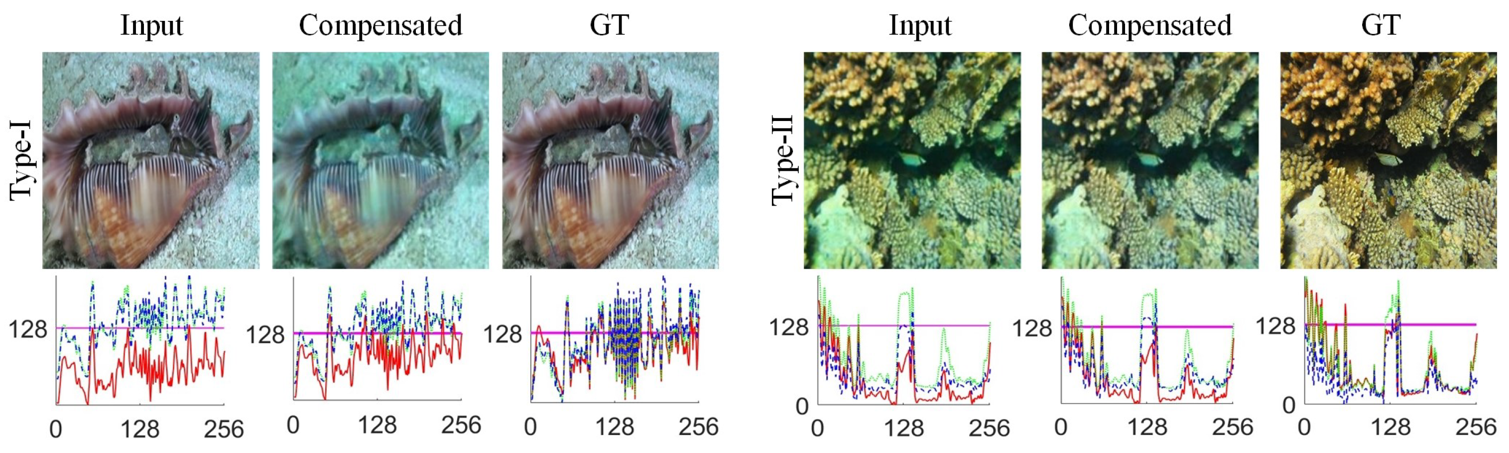
Figure 2.
Overview of the proposed framework illustrating adaptive mapping capabilities of the models: (a) Input images with intensity profiles, (b) Architecture of the Deep Line Model (DLM), (c) Examples of lines varying with parameters , (d) Output images processed by DLM, (e) Architecture of the Deep Curve Model (DCM), (f) Examples of curves demonstrating higher-order adjustments, (g) Output images processed by DCM.
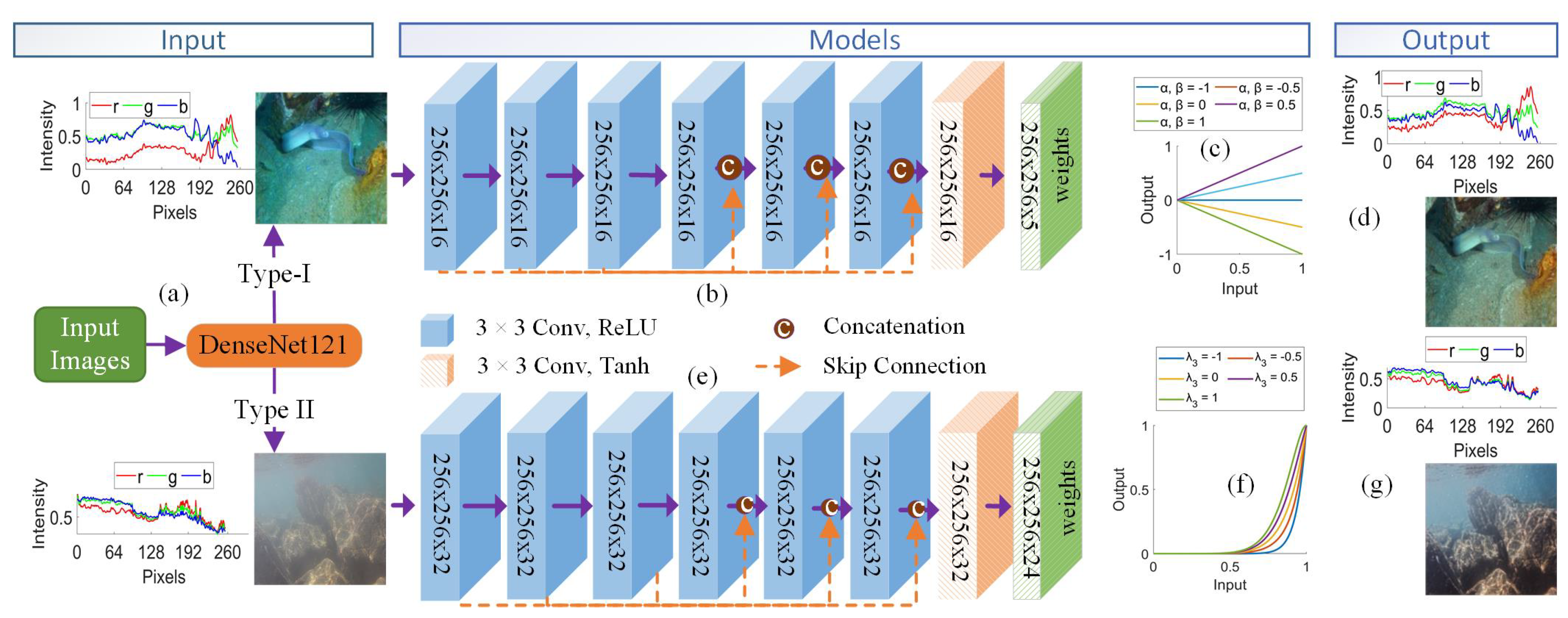
Figure 3.
Ablation study evaluating DLM and DCM for underwater image restoration. For Type-I images, DLM achieves RMSE/PSNR values of 0.05/26.73, while DCM yields 0.05/26.14 for Type-II images, and 0.06/24.80 in the UIEBD dataset, compared to DLM’s 0.16/16.10. Red boxes indicate qualitative differences between the models.
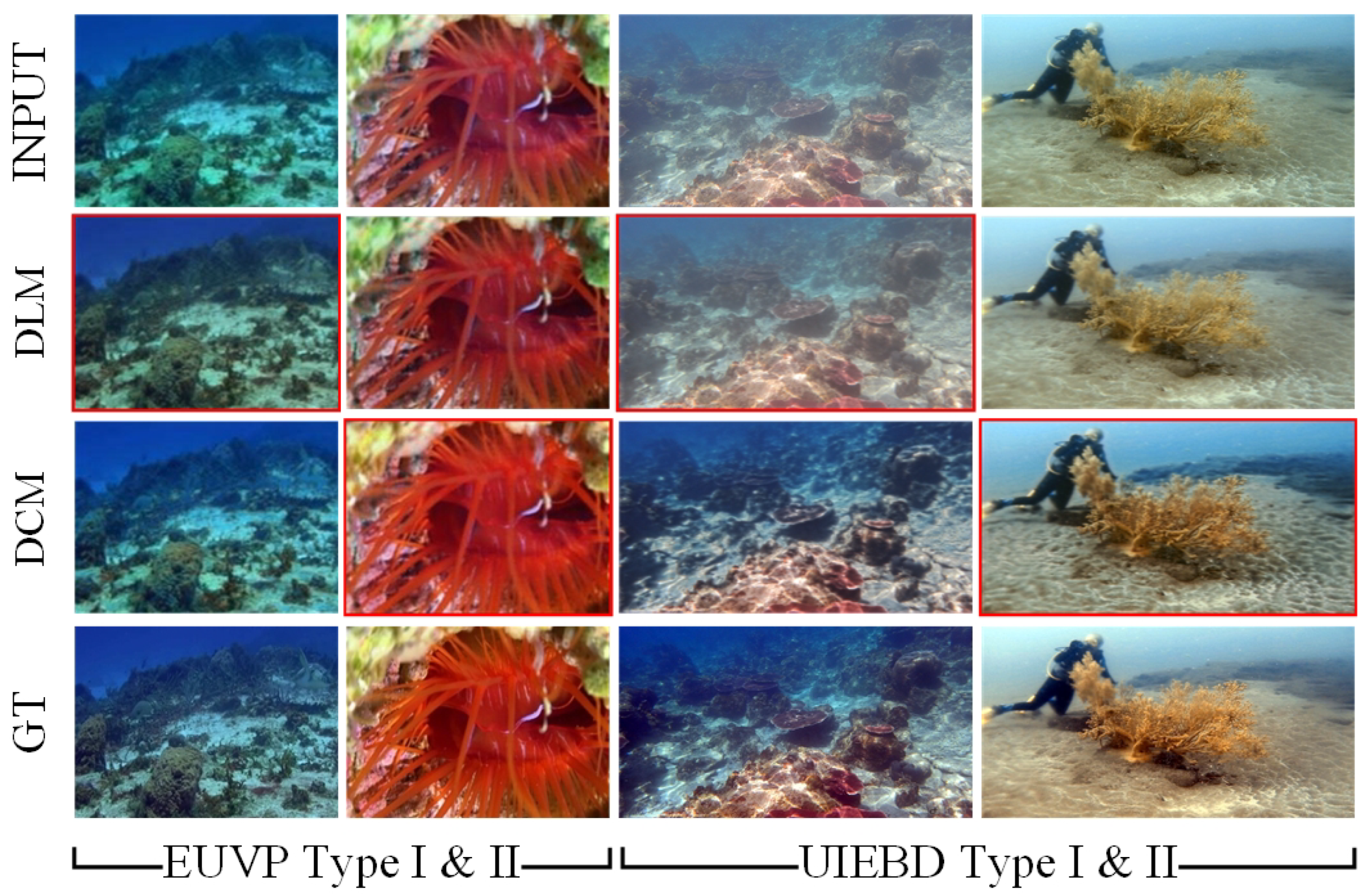
Figure 4.
Ablation study of the effect of different iterations. The RMSE/PSNR for the input and the corresponding iterations are written beneath each subfigure.
Figure 4.
Ablation study of the effect of different iterations. The RMSE/PSNR for the input and the corresponding iterations are written beneath each subfigure.
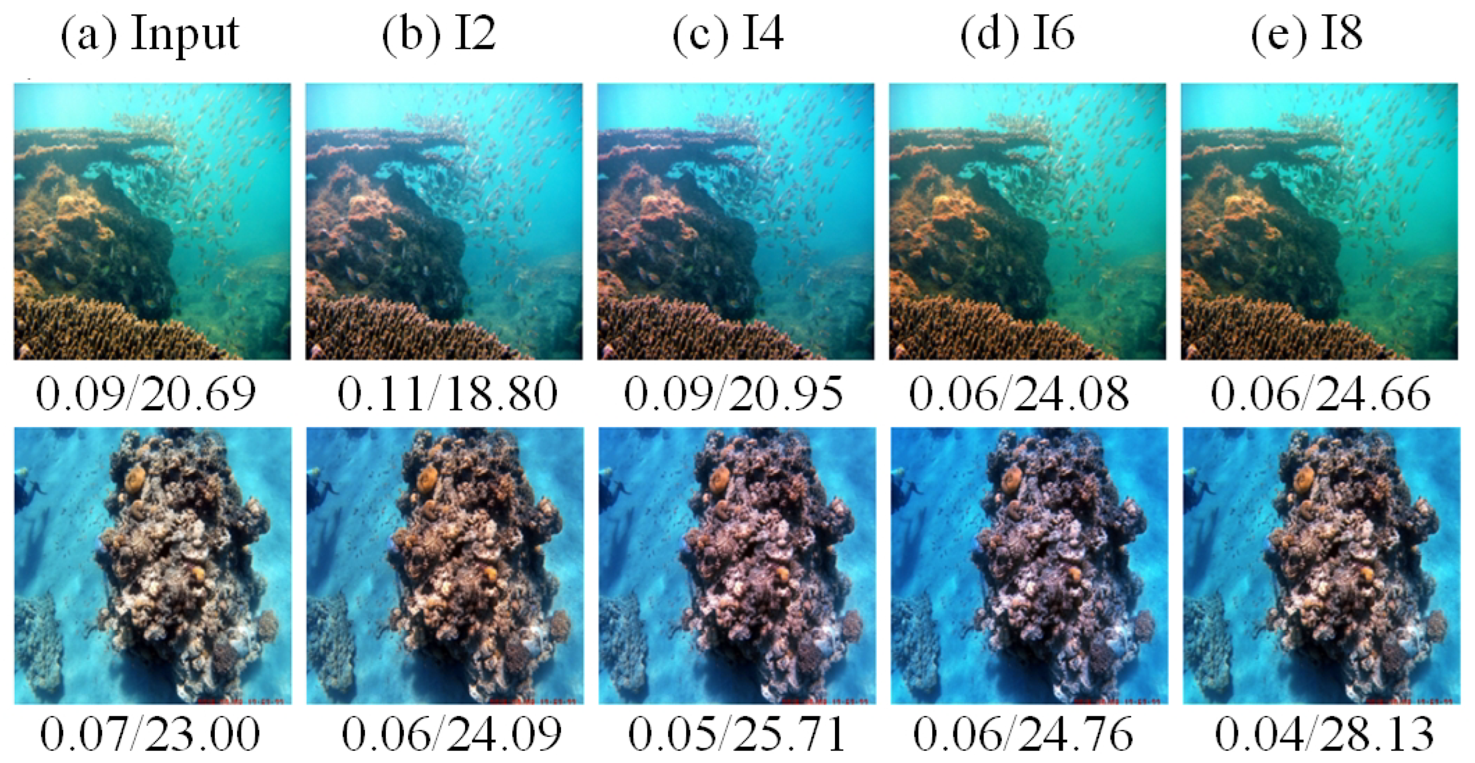
Figure 5.
Visual enhancements on the EUVP dataset utilizing non-learning and learning techniques, inclusive of our proposed method. Refer to Table for associated RMSE and PSNR values.
Figure 5.
Visual enhancements on the EUVP dataset utilizing non-learning and learning techniques, inclusive of our proposed method. Refer to Table for associated RMSE and PSNR values.
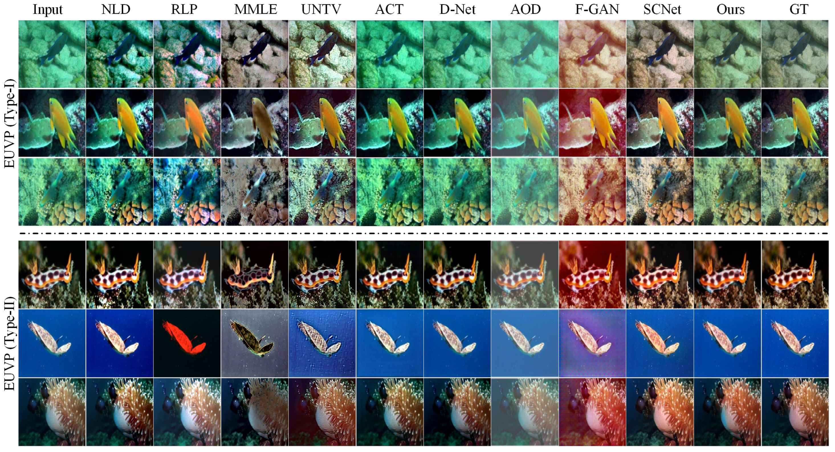
Figure 6.
Visual enhancements on the UIEBD dataset utilizing non-learning and learning techniques, inclusive of our proposed method. Refer to Table for associated RMSE and PSNR values.
Figure 6.
Visual enhancements on the UIEBD dataset utilizing non-learning and learning techniques, inclusive of our proposed method. Refer to Table for associated RMSE and PSNR values.
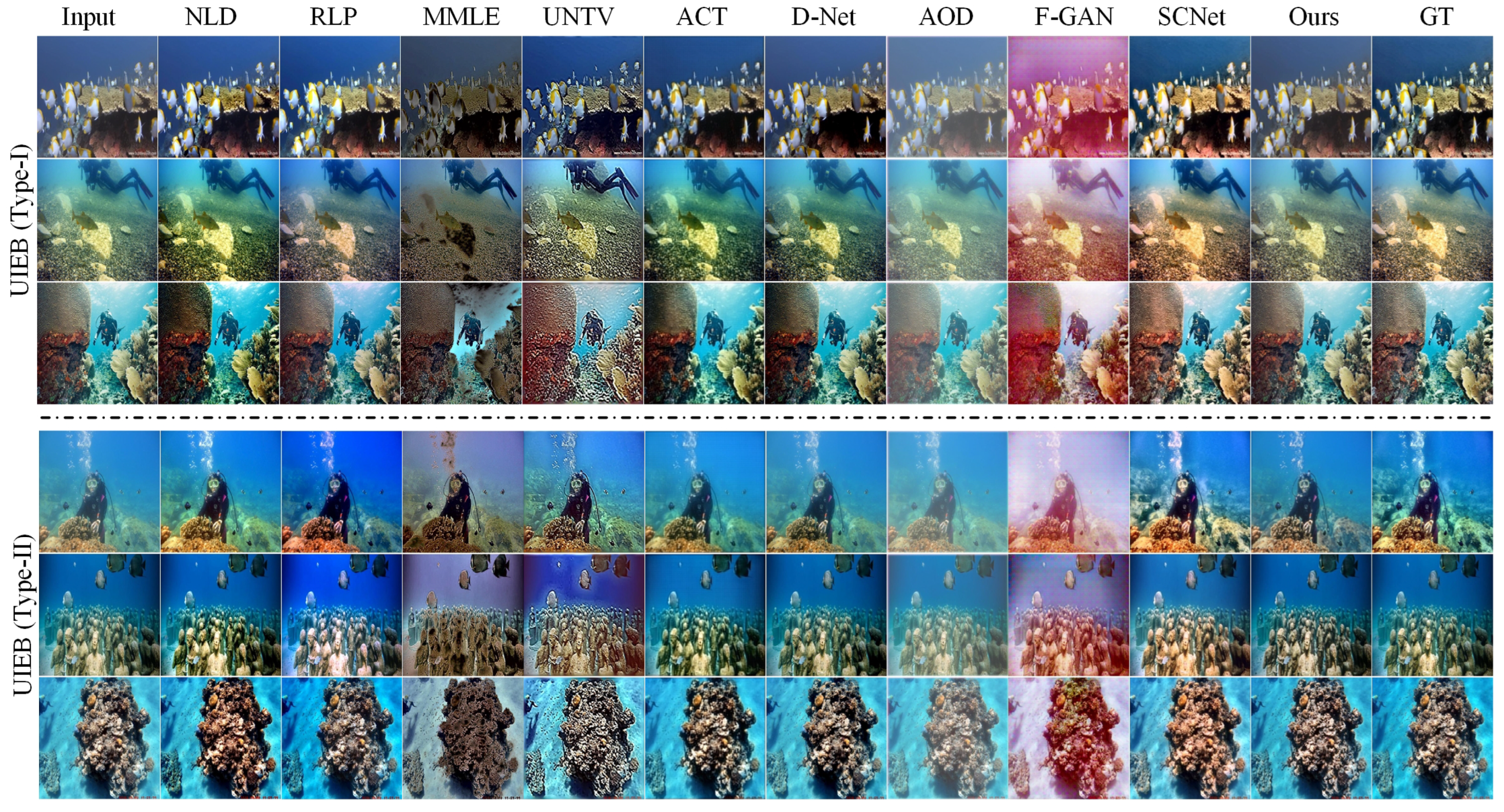
Table 1.
Quantitave results of ablation study comparing DLM and DCM. Average RMSE/PSNR for Type-I and Type-II images.
Table 1.
Quantitave results of ablation study comparing DLM and DCM. Average RMSE/PSNR for Type-I and Type-II images.
| Datasets | Group | Input | DLM | DCM |
| EUVP | Type-I | 0.11/20.00 | 0.93/22.35 | 0.89/20.63 |
| Type-II | 0.08/22.00 | 0.97/24.18 | 0.97/25.03 | |
| UIEBD | Type-I | 0.15/17.60 | 0.93/20.08 | 0.85/16.37 |
| Type-II | 0.14/18.60 | 0.94/17.81 | 0.95/22.20 |
Disclaimer/Publisher’s Note: The statements, opinions and data contained in all publications are solely those of the individual author(s) and contributor(s) and not of MDPI and/or the editor(s). MDPI and/or the editor(s) disclaim responsibility for any injury to people or property resulting from any ideas, methods, instructions or products referred to in the content. |
© 2024 by the authors. Licensee MDPI, Basel, Switzerland. This article is an open access article distributed under the terms and conditions of the Creative Commons Attribution (CC BY) license (http://creativecommons.org/licenses/by/4.0/).
Copyright: This open access article is published under a Creative Commons CC BY 4.0 license, which permit the free download, distribution, and reuse, provided that the author and preprint are cited in any reuse.


