Monitoring the Effects of Land Use Land Cover Change on Forest Biomass Carbon” in the Western Himalayan of Pakistan, a Study of Ayubia National Park

1. Introduction

The alteration of the earth's surface caused by human activities that disrupt the natural ecosystem and environmental processes of the planet is known as Land Use/Land Cover Change (LULCC) (Lambin, Turner et al. 2001). Land use change analysis necessitates a deeper comprehension of the factors that lead to LULCC, which typically entails intricately integrated sequence(Winkler, Fuchs et al. 2021). The accurate information of LULCC is of a great importance for the forests management,urbanization planning, agricultural land development, environmental management, tourism, industries and transportation etc. LULCC affect forests at both local and global level.

The loss of forest cover as a result of LULCC has led to environmental problems, global warming, habitat destruction for wildlife, and disturbance. It has also had a negative impact on the carbon content of forest biomass(Tewabe and Fentahun 2020). Remote sensing images are valuable source of spatial and temporal information to track the dynamics of LULC changes and forecast their effects on any environmental problems on a regional scale. Changes in land use and cover have become key for many different applications, including those in agriculture, the environment, ecology, forestry, geology, and hydrology, according to empirical investigations by researchers from a variety of disciplines(Hao, Zhu et al. 2021). At the same time, a significant project to study land use change has evolved as a worldwide initiative in recent decades, according to Lambin (1997), and has acquired enormous momentum in its efforts to understand the processes driving land use change. These initiatives have simulated researcher interest in using a variety of methodologies to identify and further model environmental dynamics at various levels.

LULCC planning was given significance in 1970 because of its assorted relevance after the approach of multispectral satellites pictures(Gondwe, Lin et al. 2021). An efficient and precise method for exploring terrestrial ecosystems on a large scale has been developed in recent decades as a result of advancements in remote sensing (RS) techniques(Abebe, Getachew et al. 2021). Remote sensing(RS) provides continuous temporal and spatial analyses as RS data obtained at various resolutions from different sensors can provide ecological analysis at different scales. Satellite images are periodic and cost effective allowing the researchers to conduct precise LULCC monitoring(Kumar and Arya 2021). Spatial temporal analysis of remote sensing data is also used to see the temporal patterns and identify the key drivers of deforestation(Reis 2008).

The RS data combined with the field data for validation to get precise results for LUC and LD detection and the researchers are able to carry out precise LULCC monitoring because satellite images are available on a regular basis and are inexpensive(Hassan, Shabbir et al. 2016). The key drivers of deforestation can also be identified through spatial temporal analysis of remote sensing data(Qureshi, Pariva et al. 2012).Urbanization, population growth, socioeconomic development, and forest fires are all contributing factors to the recent decline in forest biomass carbon (Sun and Liu 2019). According to(Nandal, Yadav et al. 2023), forest fires pose the greatest threat to stored terrestrial carbon, and each year, an estimated 2-3 Pg C, or 3-4 million km2 of burned forests, are released into the atmosphere.Forest fires cause changes in the world's natural and actual qualities which throughout the long term influence carbon stock(Song, Yang et al. 2021).

1.1. Materials and Methods

1.1.1. Study Area

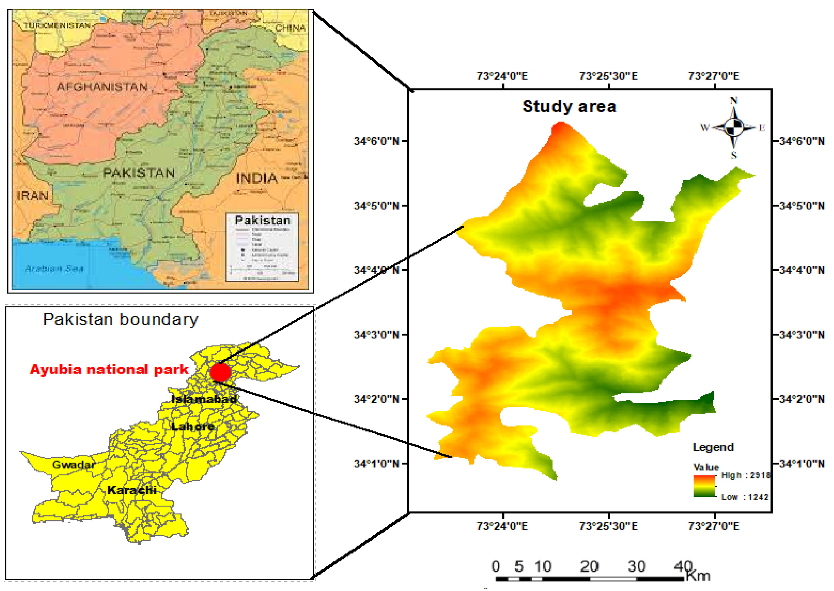
The study area Ayubia National Park is Pakistan's sole temperate coniferous forest, and it supports a wide variety of species of fragile plants and animals. In the park area, there are roughly 10 different types of Gymnosperm trees, 200 species of herbs and shrubs, and other plants. It occupies an area of 34.09 sq.km hectares and is located in Abbottabad's Galiyat Forest division between 34° 1' 45.1164" N latitude and 73° 24' 9.1836"E longitude as shown in Figure 1-1. On April 17, 1984, the region was designated as a national park and situated at the northwest corner of Murree on a series of hills that stretch north to south 1220 to 2865 meters above sea level. The highest peaks are Mukshpuri (2865m) and Mirangani (2228m), according to (Waseem, Mohammad et al. 2005). In addition to receiving precipitation in the form of substantial winter snowfall, the average annual rainfall is above 1,500 mm, and the average annual temperature is 21 C with a relative humidity of 66% (Khan 1998). Kundala, Toheedabad, Mallach, Lahurkas, Kalabun, Derwaza, Mominabad, Ram kot, Raila, and Pasala are significant settlements around the park. The substantial depletion of the vegetation in Ayubia National Park is a result of the intense population pressure from the neighboring communities.

Figure 1-1. Study Area. 

Figure 1-1. Study Area. 

1.1.2. Data Acquisition

United States Geological Survey (USGS) https://glovis.usgs.gov were used to download Landsat 5 Thematic Mapper (TM) pictures for the time periods of 1992, 2002, and 2012 as well as Landsat 8 Operational Land Imager (OLI) for 2022. Landsat 8 (OLI) includes nine bands, of which bands 1 through 7 and band 9 have a spatial resolution of 30 m, while band 8 is a panchromatic band with a spatial resolution of 15 m. The Landsat 5 TM has seven spectral bands with a spatial resolution of 30 m. Table 1-1 lists the specifics of the data sources and their specifications.

Table 1-1. Specification of Satellite sensor. 

Sensor	Year	Date	Image Resolution
Landsat 8 OLI (Path/Row:150/36, 150/37)	2022	17/10/2022	30m
Landsat 5 Imagery (Path/Row:150/36,150/37)	2012	14/7/2002	30m
Landsat 5 Imagery (Path/Row:150/36, 150/37)	2002	25/9/2002	30m
Landsat 5 TM imagery (Path/Row:150/36, 150/37)	1992	20/9/1992	30m

Table 1-1. Specification of Satellite sensor. 

Sensor	Year	Date	Image Resolution
Landsat 8 OLI (Path/Row:150/36, 150/37)	2022	17/10/2022	30m
Landsat 5 Imagery (Path/Row:150/36,150/37)	2012	14/7/2002	30m
Landsat 5 Imagery (Path/Row:150/36, 150/37)	2002	25/9/2002	30m
Landsat 5 TM imagery (Path/Row:150/36, 150/37)	1992	20/9/1992	30m

The images with the least amount of clouds (0–10%) was chosen, and it was downloaded. Table 1 provides information about the sensor specifications. As indicated in Table 2-2, the information included satellite images, digital elevation models (DEMs), topographic maps, highways, and settlement maps of the study area.

1.1.3. Land-Use Classification

With the use of a GPS Magellan Explorist 110, which represented a homogeneous class, a number of training signature polygons were first produced for each land use to be classified. The previous pattern of LULC of the studied region was determined using supervised classification algorithms with Landsat satellite data from the years 1992, 2002, 2012 and 2022. For each LULC class, the land cover area (ha) was computed. Results were produced for each year using the kappa coefficients and error matrix. The kappa coefficients, producer accuracy, total accuracy, and user accuracy for the chosen years were calculated.

Table 2-1. Land use land change categories. 

Serial no	LULC Classes	Descrption
1	Bare Land	A land with no vegetation or grasses
2	Conifer forest	Trees that grow needles instead of leaves and cones instead of flowers conifers tend to be evergreen they bear needles all year long.
3	Built-up/Settlements	Includes residential areas like town, roads,villages,strip transportation and commercial areas
4	Grassland	A grassland is an area where the vegetation is dominated by grasses with flat large area
5	Mixed Forest	Mixed forest is a vegetation type dominated by a mixture of broadleaf trees and shadow conifers.

Table 2-1. Land use land change categories. 

Serial no	LULC Classes	Descrption
1	Bare Land	A land with no vegetation or grasses
2	Conifer forest	Trees that grow needles instead of leaves and cones instead of flowers conifers tend to be evergreen they bear needles all year long.
3	Built-up/Settlements	Includes residential areas like town, roads,villages,strip transportation and commercial areas
4	Grassland	A grassland is an area where the vegetation is dominated by grasses with flat large area
5	Mixed Forest	Mixed forest is a vegetation type dominated by a mixture of broadleaf trees and shadow conifers.

1.1.4. Image Pre-Processing

Using ENVI 5.4, the satellite pictures from 1992, 2002, 2012, and 2022 were radio-metrically corrected. The top of the atmosphere (TOA) technique was used to translate the digital numbers (DNs) into radiance and reflectance. For picture correction, the equations (1-1) spectral radiance and (1-2), TOA, were applied.

$${\mathbf{L}}_{\mathsf{\lambda }}=\mathbf{G}\mathbf{a}\mathbf{i}\mathbf{n}\times \mathbf{p}\mathbf{i}\mathbf{x}\mathbf{e}\mathbf{l}\mathbf{v}\mathbf{a}\mathbf{l}\mathbf{u}\mathbf{e}+\mathbf{o}\mathbf{f}\mathbf{f}\mathbf{s}\mathbf{e}\mathbf{t}$$

(1-1)

$${\mathbf{p}}_{\mathsf{\lambda }}=\frac{\mathsf{\pi }\times {\mathbf{L}}_{\mathsf{\lambda }}\times {\mathbf{d}}^2}{{\mathbf{E}\mathbf{S}\mathbf{U}\mathbf{N}}_{\mathsf{\lambda }}\times \mathbf{s}\mathbf{i}\mathbf{n}\mathsf{\theta }}$$

(1-2)

Where ESUN_ is the solar irradiance, d is the Earth-Sun distance, L_ is the radiance, p_ is the TOA reflectance, and is the Sun elevation in degrees. Using Fast Line-of-Sight Atmospheric analysis of hypercubes (FLAASH), which lessens the impacts of humidity, haze, water vapors, aerosols, and other variables, the top of the atmosphere reflectance was then transformed to surface reflectance. The spectral signatures vary depending on the atmospheric conditions on different days. Before detecting land-use change, the conversion of TOA reflectance to surface reflectance was completed using the correct atmospheric calibration approach, as explained by (Lambin, Geist et al. 2003, Luo, Hu et al. 2022).

1.1.5. Image Classification and Accuracy

In ArcGIS 10.5, the shape file for the research region was created and the area was clipped using the topographic sheet (1:25000) from the Survey of Pakistan (SOP) as a reference. Using the Random Forest classifier approach in ArcGIS Pro 10.4, supervised classification was used to categorize various land uses. The different land cover classes of the area were represented using a stratified random approach for the accuracy evaluation of land cover maps that were separated from satellite images. Based on ground truth data and visual interpretation, the accuracy was surveyed using 200 points. An error confusion matrix was used to compare the classification results with the reference data. As it represents diagonal elements and all the components in the confusion matrix, a non-parametric Kappa coefficient was also used to quantify the degree of classification accuracy (Musetsho, Chitakira et al. 2021). Kappa is a statistic that assesses the degree to which user ratings and specified producer ratings concide. Equation 1-4 is the calculation for this:

K=P(a)-P(e)/1-p(e)

(1-4)

Where P (a) is the number of time the k raters agree, and P (e) is the number of time the k raters are expected to agree only by chance (Rijal, Rimal et al. 2021).

1.1.6. Markov Chain Model

A special and popular method for Land Use and Land Cover modeling that shows LULCC to be stochastic processes is the Markov Chain Model (Weng, 2002). According to the Markovian system, a land use system's future state is predicted based on the current situation (Araya, 2009). shift is the transformation of a system from one state to another, and the chance of this state shift is known as the Transition probability. The Markov chain is defined by the state space and the corresponding transition probabilities (Damjan, 2009). Set of states have been described in the Markov Chain model as shown in equation 2-1.

$${\mathbf{S}}_{\mathbf{t}}=\{\mathbf{S}0,\mathbf{S}1,\mathbf{S}2,\dots \dots \mathbf{S}\mathbf{n}\}$$

(2-1)

Where S_t is the current state, while in the next step it changed into S_j with transitional probabilities p_ij, the state S in the Markov Chain model could also be used for the determination of state S_t+1 in the system by using the formula given in equation 2-2, 2-3 and 2-4 (Ma C 2012).

$$\sum _{\mathit{j}=1}^{\mathit{m}}{\mathit{P}}_{\mathit{i}\mathit{j}}=1,\mathit{i},\mathit{j}=\mathrm{1,2},\dots ,\mathit{m}$$

(2-2)

$$P_{ij}=\left[\begin{array}{ccc}{p}_{11}& \cdots & p_{1n}\\ ⋮& ⋮& ⋮\\ p_{n1}& \cdots & p_{nn}\end{array}\right]$$

(2-3)

Where P_ij is the transitional probability from one land use type to another, however the value of P_ij is within the range from$1\le Pij\le 0$, where m is the land use type studied.

$${\mathbf{L}}_{\mathbf{t}+1}=\mathbf{P}\mathbf{i}\mathbf{j}\times {\mathbf{L}}_{\mathbf{t}}$$

(2-4)

Here L_t is the current land use status and t; t+1 is the time. In order to obtain both the transition and probability matrix of land use type, this study applied the Markov Chain analysis during three periods including 1992-2002, 2002-2012,2012-2022 and 2022-2040.

1.1.7. Land use Change analysis

Land use change was determined using equation 2-5.

$$\mathbf{S}\mathbf{i}=\frac{{\mathbf{L}\mathbf{U}}_{(\mathbf{i},\mathbf{t}2)}-{\mathbf{L}\mathbf{U}\mathbf{A}}_{\mathbf{i}}}{{\mathbf{L}\mathbf{U}}_{(\mathbf{i},\mathbf{t}1)}}\times \frac{1}{{\mathbf{t}}_2-{\mathbf{t}}_1}\times 100\mathbf{\%}$$

(2-5)

Si stands for change in land use, LU(i,t1) for land use change at a earlier date, LU(i,t2) for land use change at a later date, and LUAi represents areas with no change at all.

1.2. Biomass Carbon Change

Biomass carbon was assessed by field inventory in temperate coniferous forest (TCF) and Mixed forest(MF). A total 60 sample plots of 20m × 30m were taken randomly in the study area (30 plots in each forest type). In each sample plot, the diameter of all trees greater than 4 cm was measured at breast height (DBH). We measured the height of 25 trees per species, which was enough to create a DBH/height function for a particular plot. The height of the trees was measured using Abney's level. According to equation 2-6 was used to determine the volume of all trees present in the sampling sites(Williams, Phalan et al. 2018). Total biomass kgha-1 was estimated by dividing biomass by the wood density kg m-3 of a specific species in accordance with the recommendations made by the Intergovernmental Panel on Climate Change (IPCC) in 2006.

$$\mathbf{B}\mathbf{A}\left({\mathbf{m}}^2{\mathbf{h}}^{-1}\right)=\frac{\mathbf{D}\mathbf{e}\mathbf{n}\mathbf{s}\mathbf{i}\mathbf{t}\mathbf{y}}{\mathbf{h}\mathbf{a}}\times \mathbf{D}\mathbf{C}\times \mathsf{\pi }{\mathbf{r}}^2$$

(2-6)

tree volume (TV) was measured by multiplying BA and height (h) and form factor (f.f) , as shown in eq 2-11, formula(Woltz, Peneva-Reed et al. 2022).

$$\mathbf{T}\mathbf{V}\left({\mathbf{m}}^3{\mathbf{h}}^{-1}\right)=\mathbf{B}\mathbf{A}\left({\mathbf{m}}^2{\mathbf{h}}^{-1}\right)\times \mathbf{h}\left(\mathbf{m}\right)\times \mathbf{f}.\mathbf{f}$$

(2-7)

Here f.f is the volume of cylinder to actual tree form(Zeng, Liu et al. 2022) and f.f, 0.37 was used for conifers and 0.6 for broad leaved species in sub-continent as explained by(Zhou, Hartemink et al. 2019). Wood density (W.D) ton per m³ of particular species was used to calculate stem biomass (BM_S) by using equation 2-8. The W.D of each species was determined according to (Olorunfemi, Komolafe et al. 2019).

$${\mathbf{B}\mathbf{M}}_{\mathbf{S}}\left(\mathbf{M}\mathbf{g}{\mathbf{h}\mathbf{a}}^{-1}\right)=\mathbf{S}\mathbf{V}\left({\mathbf{m}}^3{\mathbf{h}}^{-1}\right)\times \mathbf{W}\mathbf{D}\left(\mathbf{M}\mathbf{g}{\mathbf{m}}^{-3}\right)$$

(2-8)

Above Ground Biomass (BM_ABG) $Mg{ha}^{-1}$was measured by using equation 2-9. The Biomass expansion factor (BEF) as described by (Kauffman, Hughes et al. 2009) is 1.51 for temperate forests of Pakistan.

AGB = Volume × Wood Density × BEF

In each sample plot, a carbon values of below-ground vegetation (BGV) sub-plot measuring 3 m by 3 m was created in order to calculate the biomass. Each plot's vegetation was first harvested, their fresh weight was noted, and the collected items were all placed into the labelled bags for subsequent examination. After 48 hours of drying in an oven at 72 °C, the samples' dried weights were calculated for biomass. Similar to how litter, dead wood, and cones in the sub-plot were gathered, they were likewise subject to the same USV for biomass carbon assessment process described above. Using a soil auger and a core sampler, three replications of the soil samples were taken from the chosen plots at depths of 0–15 cm and 15–30 cm. In the field, each soil sample was weighed and labelled. The bulk density of each soil sample was determined using a core sampler with a volume of 0.0001256 m3 (diameter = 4 cm, height = 10 cm). The soil samples were taken to the lab for further examination. The technique of soil oxidized organic carbon described by (Tiwari, Singh et al. 2019) was used to measure the amount of organic material in the soil. Utilizing a total plant biomass convertible factor, which represents the average biomass content of the plant, carbon was calculated. The carbon content of all plant biomass, as determined by this conversion factor, is estimated to be 50% (Rashid, Bhat et al. 2017). According to (Morreale, Thompson et al. 2021) the bulk density, carbon concentration, and layer thickness were multiplied to get the soil's (MgC ha-1) carbon values.

1.2.1. Carbon Loss Assessment

The deforestation resulted in the conversion of forestland into grassland and built-up.Change in carbon is determined by Equation 2-10 (Gandhi and Sundarapandian 2017).

$$∆\mathbf{C}={\mathbf{T}\mathbf{o}\mathbf{t}\mathbf{a}\mathbf{l}\mathbf{F}\mathbf{o}\mathbf{r}\mathbf{e}\mathbf{s}\mathbf{t}\mathbf{C}\mathbf{a}\mathbf{r}\mathbf{b}\mathbf{o}\mathbf{n}}_{\mathbf{t}2}-{\mathbf{T}\mathbf{o}\mathbf{t}\mathbf{a}\mathbf{l}\mathbf{F}\mathbf{o}\mathbf{r}\mathbf{e}\mathbf{s}\mathbf{t}\mathbf{C}\mathbf{a}\mathbf{r}\mathbf{b}\mathbf{o}\mathbf{n}}_{\mathbf{t}1}$$

(2-10)

The annual rate of carbon loss is determined by Equation 4-6:

$$\mathsf{\Delta }\mathbf{C}=\frac{{(\mathbf{T}\mathbf{o}\mathbf{t}\mathbf{a}\mathbf{l}\mathbf{F}\mathbf{o}\mathbf{r}\mathbf{e}\mathbf{s}\mathbf{t}\mathbf{C}\mathbf{a}\mathbf{r}\mathbf{b}\mathbf{o}\mathbf{n}}_{\mathbf{t}2}-{\mathbf{T}\mathbf{o}\mathbf{t}\mathbf{a}\mathbf{l}\mathbf{F}\mathbf{o}\mathbf{r}\mathbf{e}\mathbf{s}\mathbf{t}\mathbf{C}\mathbf{a}\mathbf{r}\mathbf{b}\mathbf{o}\mathbf{n}}_{\mathbf{t}1})}{{(\mathbf{t}}_2-{\mathbf{t}}_1)}$$

(2-11)

1.3. Results and Analysis

ΔC = Carbon loss or gain

TFC_t2 = Total forest carbon at time t₂

TFC_t1 = Total forest carbon at time t₁

1.3.1. Land Use Land Change Analysis

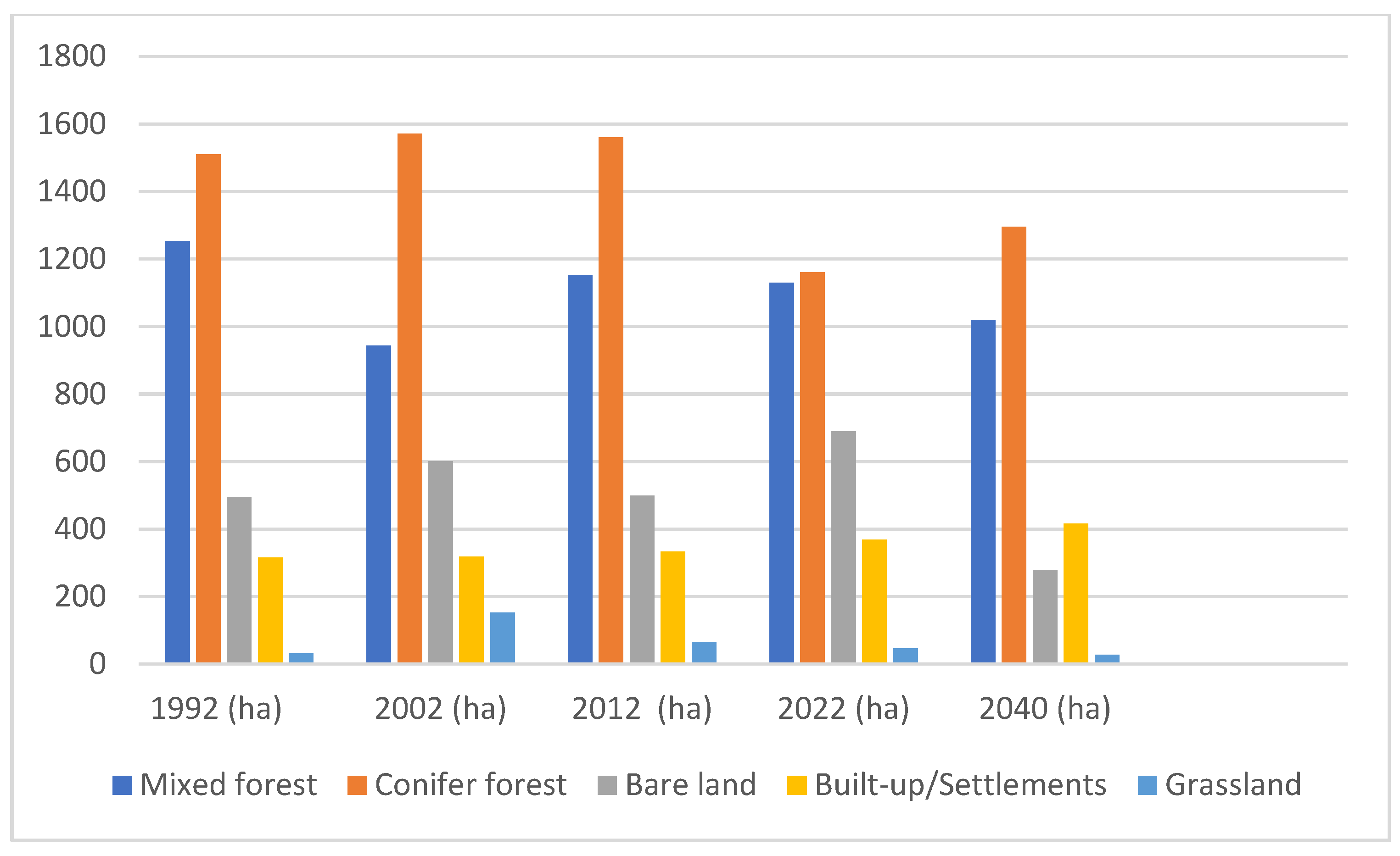
The results of LULCC showed that the Mixed forest decreased from 1253.79 (ha) in 1992 to 943.21 (ha) in 2002 with -0.75% loss. In 2022 conifer forest reduced from 1510.2 (ha) to 1161.09 ha or approximately -76.8%. Similarly, the bare land reduced from 601.65 ha in 2002 to 499.79 ha in 2012. In 2022 it increased to 689.13 (ha) In 2022 conifer forest reduced from 1510.2 (ha) to 1161.09 ha or approximately -76.8% and for it was projected to 1295.45 (ha) in 2040. Similarly, the mixed forest slighlty increased from 943.21 ha in 2002 to 1152.74 ha in 2012. On the other hand, from 1129.71 (ha) in 2022, mixed forest were projected to reduce to 1019.56 (ha) in 2040 see Table 3-1, 4-1 and Figures 2-1,2-1a.

Table 3-1. LULCC Statistics for different years.

Land use	1992 (ha)	2002 (ha)	2012 (ha)	2022 (ha)	2040 (ha)
Mixed forest	1253.79	943.21	1152.74	1129.71	1019.56
Conifer forest	1510.20	1570.32	1560.06	1161.09	1295.45
Bare land	493.56	601.65	499.79	689.13	278.76
Built-up/Settlements	315.06	317.97	332.78	368.23	416.29
Grassland	31.6	152.37	65.79	46.71	27.54

Table 3-1. LULCC Statistics for different years.

Land use	1992 (ha)	2002 (ha)	2012 (ha)	2022 (ha)	2040 (ha)
Mixed forest	1253.79	943.21	1152.74	1129.71	1019.56
Conifer forest	1510.20	1570.32	1560.06	1161.09	1295.45
Bare land	493.56	601.65	499.79	689.13	278.76
Built-up/Settlements	315.06	317.97	332.78	368.23	416.29
Grassland	31.6	152.37	65.79	46.71	27.54

Table 4-1. (%) Statistics of LULCC per decade and annual.

Land use categories	1992-2002 change (%)	Annual change (%)	2002-2012 change (%)	Annual change (%)	2012-2022 change (%)	Annual change (%)	2022-2040 change (%)	Annual change (%)
Mixed forest	-16.7	-0.167	+10.49	+0.104	+18.3	+0.183	+16.47	+0.164
Conifer forest	+3.98	+0.039	-0.65	-0.0065	-25.57	-0.255	+11.57	+0.11
Bare land	+25.7	+0.257	-14.6	-0.146	+30.07	+0.30	-59.4	- 0.59
Built-up/settlements	+0.92	+0.09	-10.12	-0.101	+13.80	+0.138	+34.18	+0.341
Grassland	+65.3	+0.653	+25.62	+0.256	-29.00	-0.290	-41.04	-0.410

Table 4-1. (%) Statistics of LULCC per decade and annual.

Land use categories	1992-2002 change (%)	Annual change (%)	2002-2012 change (%)	Annual change (%)	2012-2022 change (%)	Annual change (%)	2022-2040 change (%)	Annual change (%)
Mixed forest	-16.7	-0.167	+10.49	+0.104	+18.3	+0.183	+16.47	+0.164
Conifer forest	+3.98	+0.039	-0.65	-0.0065	-25.57	-0.255	+11.57	+0.11
Bare land	+25.7	+0.257	-14.6	-0.146	+30.07	+0.30	-59.4	- 0.59
Built-up/settlements	+0.92	+0.09	-10.12	-0.101	+13.80	+0.138	+34.18	+0.341
Grassland	+65.3	+0.653	+25.62	+0.256	-29.00	-0.290	-41.04	-0.410

Figure 2-1. LULCC map (a) 1992, (b) 2002, (c) 2012 and (d) 2022.

Figure 2-1. LULCC map (a) 1992, (b) 2002, (c) 2012 and (d) 2022.

Figure 2-1(a). LULCC map (a) projected 2022, (b) predicted 2040.

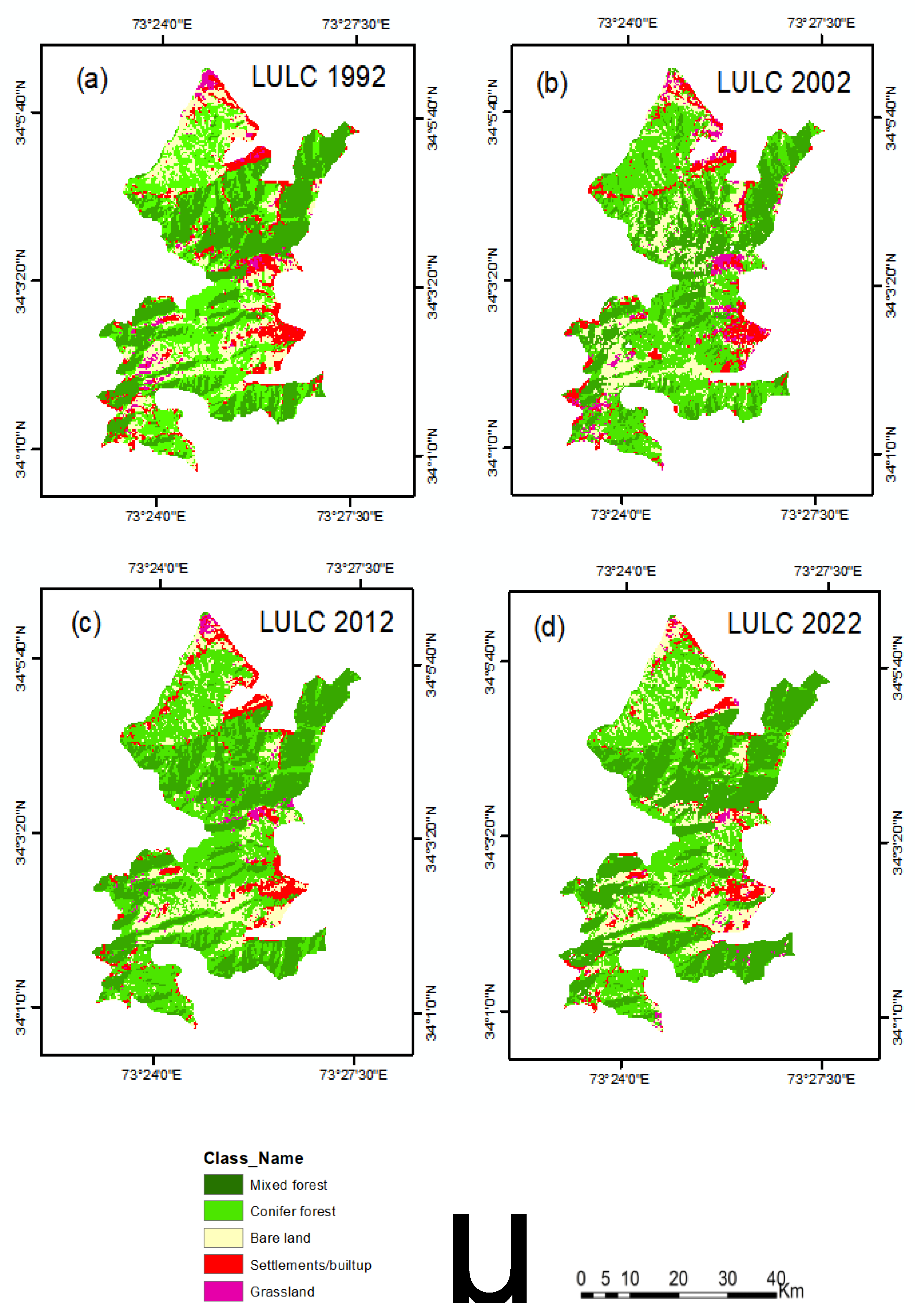
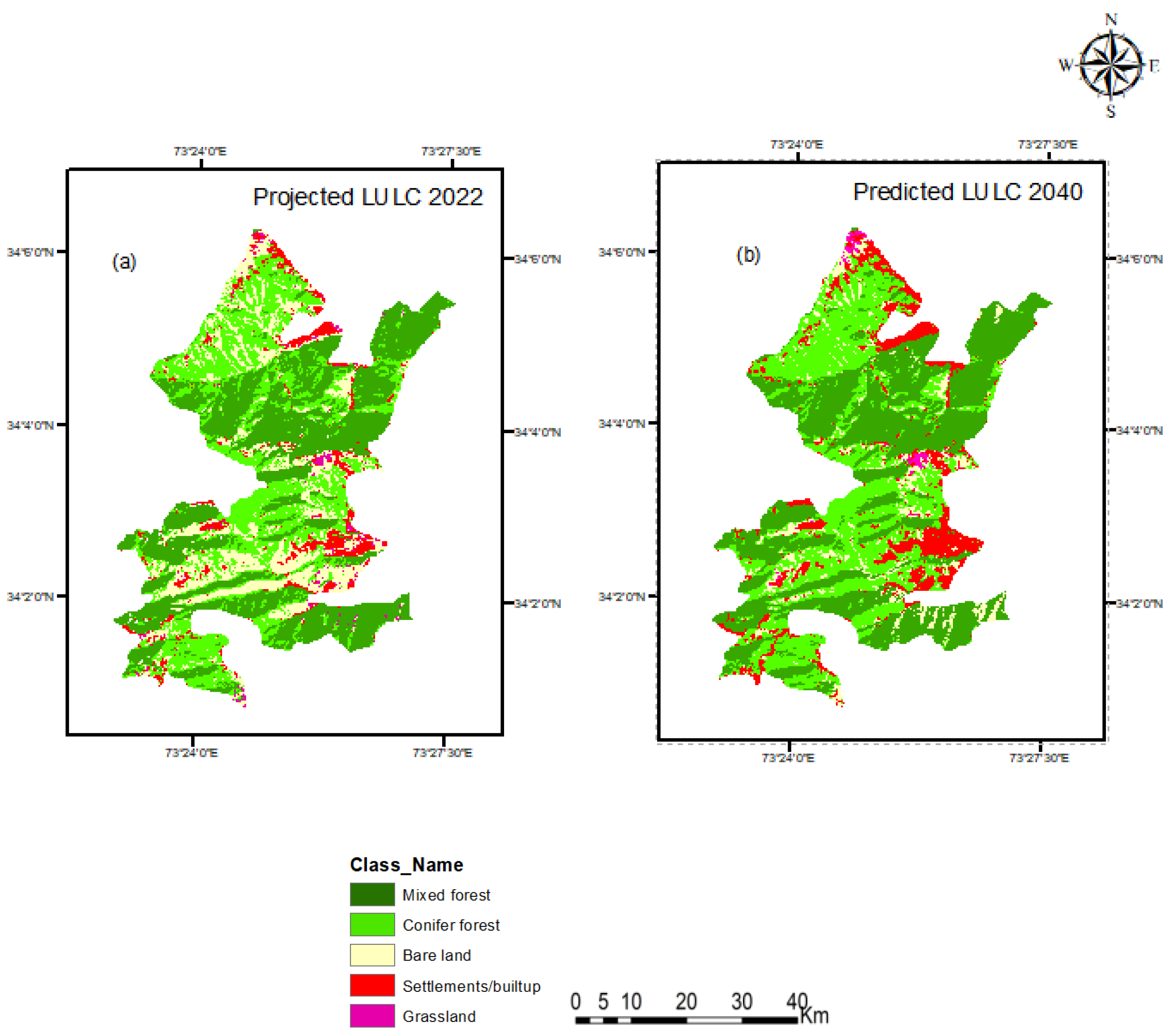
Figure 2-1(a). LULCC map (a) projected 2022, (b) predicted 2040.

The results showed that during the period 1992-2002, CF decrease by 24.7% (0.247% yr^-1), during 2002-2022, Mixed forest increased by 10.495 (0.104% yr^-1,) and 8.13% (0.183% yr^-1), respectively as shown in Table 4-1. Apart from a decrease and slightly increased in area under Mixed forest, major changes were also observed for BL CF, GL and SM (Table 4-1 and Figure 2-1,2-2). Our results showed that a total of 371.94 ha forest land (CF, MF) has been converted into other land uses from 1992 to 2022 and Indicating the increasing scale of anthropogenic pressure on forest resources of the Park. During the predicted period 2022-2040 the built up area may increase more due to population growth and economic factors.

Figure 2-2. Carbon Pool. 

Figure 2-2. Carbon Pool. 

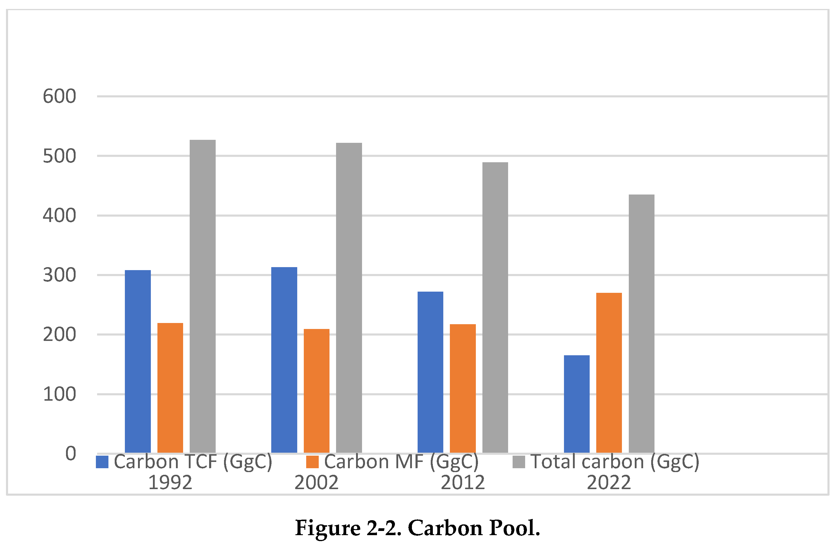
Table 5-1. LUC statistics from 1992 to 2022. 

Land use type	Land use changes to other land uses	Area change (ha) (1992-2022)	Total area change (ha)
Conifer forest	Bare land	104.94	472.95
	Mixed forest	241.92
	Settlement	126.09
Mix forest	Bare land	7.740	61.7
	Settlements	5.490
	Conifer forest	48.51
Built-up/Settlements	Mixed forest	0.81	29.34
	Bare land	22.86
	Grassland	5.67
Grassland	Conifer forest	2.340	25.11
	Bare land	14.40
	Settlements	8.37

Table 5-1. LUC statistics from 1992 to 2022. 

Land use type	Land use changes to other land uses	Area change (ha) (1992-2022)	Total area change (ha)
Conifer forest	Bare land	104.94	472.95
	Mixed forest	241.92
	Settlement	126.09
Mix forest	Bare land	7.740	61.7
	Settlements	5.490
	Conifer forest	48.51
Built-up/Settlements	Mixed forest	0.81	29.34
	Bare land	22.86
	Grassland	5.67
Grassland	Conifer forest	2.340	25.11
	Bare land	14.40
	Settlements	8.37

1.3.2. Accuracy Assessment of LULCC

The results showed kappa coefficient 0.845, 0.862, 0.873 and 0.928 for the year 1992, 2002, 2012 and 2022 respectively shown in Table 5-2. The simulated results showed kappa statistics values to range from 0.7044 to 0.9086. while transitional matrix statistics for 2022 are shown in Table 5-3.

Table 5-2. Accuracy Assessment for 1992-2022.

Classified map	Overall Accuracy	Kappa Coefficient
LULC map 1992	86.81 %	0.845
LULC map 2002	89.43%	0.862
LULC map 2012	90.43%	0.873
LULC map 2022	94.08%	0.928

Table 5-2. Accuracy Assessment for 1992-2022.

Classified map	Overall Accuracy	Kappa Coefficient
LULC map 1992	86.81 %	0.845
LULC map 2002	89.43%	0.862
LULC map 2012	90.43%	0.873
LULC map 2022	94.08%	0.928

The results from model validation also showed the total agreement was 0.93, while the simulation error was 0.82 as shown in Table 5-2a, while the probability transitional matrix statistics for 2022 are shown in Table 5-3.

Table 5-2a. Validation results and Agreement/Disagreement.

Agreement/Disagreement (%)
Allocation disagreement	7.45
Quantity disagreement	5.16
Allocation agreement	14.95
Quantity agreement	62.10
Chance agreement	10.34

Table 5-2a. Validation results and Agreement/Disagreement.

Agreement/Disagreement (%)
Allocation disagreement	7.45
Quantity disagreement	5.16
Allocation agreement	14.95
Quantity agreement	62.10
Chance agreement	10.34

Table 5-3. Transition matrix, simulation for LULCC in year 2022.

	Probability to change from-to
	Mixed forest	Conifer forest	Bare land	Built-up/Settlements	Grassland
Mixed forest	0.8836	0.1014	0.0108	0.0030	0.0012
Conifer forest	0.2726	0.6831	0.0367	0.0006	0.0071
Bare land	0.1178	0.2279	0.5990	0.0082	0.0471
Builtup/Settlements	0.0012	0.4710	0.1765	0.2796	0.0718
Grassland	0.0000	0.0000	0.7272	0.0000	0.2728

Table 5-3. Transition matrix, simulation for LULCC in year 2022.

	Probability to change from-to
	Mixed forest	Conifer forest	Bare land	Built-up/Settlements	Grassland
Mixed forest	0.8836	0.1014	0.0108	0.0030	0.0012
Conifer forest	0.2726	0.6831	0.0367	0.0006	0.0071
Bare land	0.1178	0.2279	0.5990	0.0082	0.0471
Builtup/Settlements	0.0012	0.4710	0.1765	0.2796	0.0718
Grassland	0.0000	0.0000	0.7272	0.0000	0.2728

1.3.3. Carbon Dynamics

The estimated carbon value recorded in TCF is 135.19 ±9.74 MgC ha^-1, whereas it is in 86.43 ±8.25 MgC ha^-1 in MF (Table 6-1). In each forest, the higher value of carbon is recorded for Above ground vegetation (ABGV) followed by soil, below ground vegetation and litter dead wood. The results of the total carbon stock (Table 6-2) and Figure 2-2 showed that in 1992 the total forest carbon stock was 527 GgC. Similarly, the total forest carbon stock was reduced in 2002, 2012 and 2022 i.e. 522 GgC, 489 GgC, and 435 GgC respectively. These findings revealed the decreasing trend in carbon value associated with LULC.

Table 6-1. Carbon Inventory results. 

Carbon pool	Temperate conifer forest (MgC∙ha-1)	Mixed forest (MgC∙ha-1)
Above ground	90.71 ±31.96	34.31 ±18.76
Below ground	1.93 ±0.22	1.53 ±0.48
Litter and dead wood	1.27 ±0.37	0.88 ±0.36
Soil carbon	49.72 ±9.47	46.24 ±8.92
Total carbon	135.19 ±9.74	86.43 ±8.25

Table 6-1. Carbon Inventory results. 

Carbon pool	Temperate conifer forest (MgC∙ha-1)	Mixed forest (MgC∙ha-1)
Above ground	90.71 ±31.96	34.31 ±18.76
Below ground	1.93 ±0.22	1.53 ±0.48
Litter and dead wood	1.27 ±0.37	0.88 ±0.36
Soil carbon	49.72 ±9.47	46.24 ±8.92
Total carbon	135.19 ±9.74	86.43 ±8.25

Table 6-2. Total stored carbon. 

	Temperate coniferous forest (ha)	Mixed forest (ha)	Carbon TCF (GgC)	Carbon MF (GgC)	Total carbon (GgC)
1992	1510.20	1253.79	308	219	527
2002	1570.32	943.21	313	209	522
2012	1560.06	1152.74	272	217	489
2022	1161.09	1019.56	165	270	435

Table 6-2. Total stored carbon. 

	Temperate coniferous forest (ha)	Mixed forest (ha)	Carbon TCF (GgC)	Carbon MF (GgC)	Total carbon (GgC)
1992	1510.20	1253.79	308	219	527
2002	1570.32	943.21	313	209	522
2012	1560.06	1152.74	272	217	489
2022	1161.09	1019.56	165	270	435

1.4. Discussion and Conclusion

1.4.1. Land Use Land Cover and Carbon Change

In Pakistan's temperate and subtropical areas, where LULC and deforestation are ongoing processes, natural forests are primarily found. The rise in SM and BL between 1992 and 2022 reveals the extent of LULC in the park. In comparison to our base year 1992, we discovered that SM has grown by 25.9% during the past 30 years. According to Figure 2-3, the SM for Ayubia increased from 315.06 to 368.23 between 1992 and 2022. Additionally, the number of SM in and around the park during 2022-2040 will increase more due to settlement growth(Waseem, Mohammad et al. 2005).

Figure 2-3. LULC class changes. 

Figure 2-3. LULC class changes. 

For instance, the CF decreased from 1510.2 hectares in the base year 1992 to 1161.09 ha in 2022. This downward trend in CF is comparable to that noted by Malik and Husain (2003; 48.4% in 1994, 54.8% in 2000). The uncontrolled and illegal logging by local villages for fuelwood, livestock grazing, and forest fires may be to blame for the transformation of CF into BL in and around the park. As is the case elsewhere in the world, forest fires frequently occur in ANP, particularly during the dry summer months(Ahmad and Javed 2007). These fires usually damage the CF more severely as compared to MF. The continuous reduction in the area under CF and increase in areas under BL and SM showed CF to have been mainly converted into BL, GL and SM.

Carbon was computed with values ranging from 86.43 ± 8.25 in MF to 135.19 ± 9.74 in TCF. Similar findings were reported for the carbon store in the temperate woods of Nathiagali(Amir, Muhammad et al. 2022). Similarly, the stated figure by (Gandhi and Sundarapandian 2017) from the Indian Himalayan area conflicts with our current findings. The loss of carbon due to the conversion of forestland to other land uses decreased from 527 GgC in 1992 to 435 GgC in 2022. The same findings were previously published and demonstrated a loss of 32.7 PgC from Brazil's Amazonian protected areas in 2014(MohanRajan, Loganathan et al. 2020). Similar to this, more than 3 million km² of US protected areas' forest, grassland, and shrubland were converted to agricultural land between 1700 and 2005, resulting in a 10,607 TgC loss(Núñez-Regueiro, Siddiqui et al. 2021) . This decrease in carbon corroborates the idea that forest land's capacity to store carbon is diminished as a result of conversion to other land uses. Forest conversion brought about by deforestation, agricultural development, and settlement growth linked to population increase led to a drop in carbon stock. Over these different periods, the highest rate of carbon losses was recorded for the period 2012-2022 as shown in Table 6-3. This period also coincided with the maximum of population growth and human migration within the study area. Although this LULC affects carbon loss, the intensity is much higher where CF is converted into SM, or BL (Ohler, Schreiner et al. 2023).

Table 6-3. Forest carbon loss. 

	Total carbon loss/gain (MgC)		Net carbon loss (MgC)	Net annual carbon loss (MgC∙yr-1)
	TCF	MF
1992-2002	435.12	-140	295.12	29.5
2002-2012	410	+120	530	53.0
2012-2022	325	270	595	59.5

Table 6-3. Forest carbon loss. 

	Total carbon loss/gain (MgC)		Net carbon loss (MgC)	Net annual carbon loss (MgC∙yr-1)
	TCF	MF
1992-2002	435.12	-140	295.12	29.5
2002-2012	410	+120	530	53.0
2012-2022	325	270	595	59.5

Between 1992 and 2022, Ayubia's population grew from 18,000 to nearly 55000,000. In addition to other environmental and socioeconomic issues, these demographic characteristics are the main causes of LUC in and around ANP (PKS 2019). Additionally, it was predicted that 16,000 people lived in nearby villages in 1992, but by 2022, this number had grown to almost 55,000, spread across 12 communities (Iqbal and Khan 2014). The viability of these natural environments is also seriously threatened by this demographic strain (Li, Yang et al. 2018, Ohler, Schreiner et al. 2023). The growth of built-up regions and the extraction of wood (fuel wood, artisanal, and commercial logging) are also influenced by this demographic pressure and contribute to the alteration of the forest cover and the deterioration of natural ecosystems(Jiyuan, Mingliang et al. 2002, Justice, Gutman et al. 2015). Anthropogenic activities pose serious hazards to the world's forest cover, according to several research (Rokityanskiy, Benítez et al. 2007, Sasmito, Taillardat et al. 2019). Historically, this increase in population and other underlying factors particularly in developing countries have been observed to be the most important driving force of LULC (Rosero-Bixby and Palloni 1998). According to (Tan, Ge et al. 2023), these underlying drivers of LULC are poverty, population growth, and socio-economic situation. Increased population often results in the migration of people in search of farmlands and forests are easier to convert to agricultural land(Luo, Hu et al. 2022). Rural areas around the ANP have experienced unchecked urban growth, which has forced these areas' rural areas into the region's wooded areas. Because National Parks feature high-quality limestone and sandstone needed for cement manufacture, stone mining for this purpose also contributes to carbon loss (Avtar, Tsusaka et al. 2020). Around the ANP, there are over 300 stone quarries, which have a negative impact on the flora, fauna, and 58 kinds of animals and over 900 plant species (The News, july 13, 2014). In a related research,(Khan, Khan et al. 2021) found that the primary causes of deforestation in the ANP region were uncontrolled harvesting, forest disease, and the removal of wood for commercial and domestic use.

Due to falling dry needles from conifer forests throughout the summer and dry season around May, forest fires frequently happen in the ANP. According to (de Groot, et al. 2009), the amount of carbon lost each year as a result of forest fires ranges from 50.2% to 57.6%, depending on the intensity of the fire. The majority of forest fires that started in Pakistan's temperate woods were unintentional as a result of carelessness and leisure activities. In Pakistan's temperate woods, surface fires have been seen to be trending upward(Amir, Muhammad et al. 2022). According to (Kauffman, Hughes et al. 2009), forest fires are known to decrease soil carbon, soil erosion, understory vegetation, and soil bareness. Livestock grazing and trampling have a negative impact on plant regeneration and contribute to LULC(Ahmad and Nizami 2015).

The research also covered the main causes of land use change and carbon loss in ANP, such as the exploitation of fuel wood for commercial purposes, population pressure and SM growth, which have a negative impact on the park's environment. Additionally, decreased forest area is a result of the construction of new infrastructure. These elements, when combined with lack governmental regulations and poor land use management strategies, encourage a decline in the amount of carbon stored in the ANP's forest biomass. This deforestation process may be slowed down, stopped, and even reversed by better forest management, sensible forest conservation laws, the creation of land use management plans, and urbanization controls.

1.4.2. Conclusion

Interpretation of multi temporal satellite imagery was found to be a practical method for determining the dynamics of land use change. For the years 1992, 2002, 2012, and 2022, Geographic Information System (GIS) tools were used to analyze the land use change patterns of Ayubia National Park (ANP) present in the study area. The results showed that the area under Mixed forest increased slightly while the area under conifer forest decreased continuously. According to the carbon shift dynamics of ANP, the area covered by conifer forests decreased by 25.57 percent (or 0.25 percent per year) from 1992 to 2022.It is predicted that the builtup area will increased to 416.79 ha in 2040 which decreasse the forestland from 1510.20 in intial period to 1295.45 ha in 2040 and mixed forest from 1253.79 to 1019.56 in 2040.Similarly, settlements increased by 13.80% (0.13% yr^-1) respectively, during the same period. The conversion of forests into other land uses resulted in the reduction of carbon value highlighting that land use change significantly alters carbon dynamics of the Park. The information derived from this study could assist in the development of appropriate sustainable forest management policies in the western Himalayan region of Pakistan.

References

- Abebe, G., D. Getachew and A. Ewunetu (2021). "Analysing land use/land cover changes and its dynamics using remote sensing and GIS in Gubalafito district, Northeastern Ethiopia." SN Applied Sciences 4(1): 30.
- Ahmad, A. and S. M. Nizami (2015). "Carbon stocks of different land uses in the Kumrat valley, Hindu Kush Region of Pakistan." Journal of forestry research 26: 57-64.
- Ahmad, S. S. and S. Javed (2007). "Exploring the economic value of underutilized plant species in Ayubia National Park." Pakistan Journal of Botany 39(5): 1435-1442.
- Ali, A.; Muhammad, S.; Nawaz, H.; Tayyab, M.; Awan, U.F.; Rasool, K.; Khan, Z.-U. Growth response of four dominant conifer species in moist temperate region of Pakistan (Ayubia National Park). Not. Bot. Horti Agrobot. Cluj-Napoca 2022, 50, 12674–12674, . [CrossRef]
- Avtar, R.; Tsusaka, K.; Herath, S. Assessment of forest carbon stocks for REDD+ implementation in the muyong forest system of Ifugao, Philippines. Environ. Monit. Assess. 2020, 192, 1–18, . [CrossRef]
- Gandhi, D.S.; Sundarapandian, S. Large-scale carbon stock assessment of woody vegetation in tropical dry deciduous forest of Sathanur reserve forest, Eastern Ghats, India. Environ. Monit. Assess. 2017, 189, 187, . [CrossRef]
- Gondwe, J.F.; Lin, S.; Munthali, R.M. Analysis of Land Use and Land Cover Changes in Urban Areas Using Remote Sensing: Case of Blantyre City. Discret. Dyn. Nat. Soc. 2021, 2021, 1–17, . [CrossRef]
- Hao, S.; Zhu, F.; Cui, Y. Land use and land cover change detection and spatial distribution on the Tibetan Plateau. Sci. Rep. 2021, 11, 1–13, . [CrossRef]
- Hassan, Z.; Shabbir, R.; Ahmad, S.S.; Malik, A.H.; Aziz, N.; Butt, A.; Erum, S. Dynamics of land use and land cover change (LULCC) using geospatial techniques: a case study of Islamabad Pakistan. SpringerPlus 2016, 5, 1–11, . [CrossRef]
- Iqbal, M.F.; Khan, I.A. Spatiotemporal land use land cover change analysis and erosion risk mapping of Azad Jammu and Kashmir, Pakistan. Egypt. J. Remote Sens. Space Sci. 2014, 17, 209–229, https://doi. org/10.1016/j.ejrs.2014.09.004.
- Jiyuan, L.; Mingliang, L.; Xiangzheng, D.; Dafang, Z.; Zengxiang, Z.; Di, L. The land use and land cover change database and its relative studies in China. J. Geogr. Sci. 2002, 12, 275–282, . [CrossRef]
- Justice, C.; Gutman, G.; Vadrevu, K.P. NASA Land Cover and Land Use Change (LCLUC): An interdisciplinary research program. J. Environ. Manag. 2015, 148, 4–9, . [CrossRef]
- Kauffman, J. B., R. F. Hughes and C. Heider (2009). "Carbon pool and biomass dynamics associated with deforestation, land use, and agricultural abandonment in the neotropics." Ecol Appl 19(5): 1211-1222.
- Khan, I.A.; Khan, W.R.; Ali, A.; Nazre, M. Assessment of Above-Ground Biomass in Pakistan Forest Ecosystem’s Carbon Pool: A Review. Forests 2021, 12, 586, . [CrossRef]
- Kumar, S.; Arya, S. Change Detection Techniques for Land Cover Change Analysis Using Spatial Datasets: a Review. Remote. Sens. Earth Syst. Sci. 2021, 4, 172–185, . [CrossRef]
- Lambin, E.F.; Geist, H.J.; Lepers, E. Dynamics of Land-Use and Land-Cover Change in Tropical Regions. Annu. Rev. Environ. Resour. 2003, 28, 205–241, . [CrossRef]
- Lambin, E.F.; Turner, B.L.; Geist, H.J.; Agbola, S.B.; Angelsen, A.; Bruce, J.W.; Coomes, O.T.; Dirzo, R.; Fischer, G.; Folke, C.; et al. The causes of land-use and land-cover change: Moving beyond the myths. Glob. Environ. Chang. 2001, 11, 261–269, doi:10.1016/s0959-3780(01)00007-3.
- Li, X.L.; Yang, L.X.; Tian, W.; Xu, X.F.; He, C.S. Land use and land cover change in agro-pastoral ecotone in Northern China: A review.. 2018, 29, 3487–3495.
- Luo, M.; Hu, G.; Chen, G.; Liu, X.; Hou, H.; Li, X. 1 km land use/land cover change of China under comprehensive socioeconomic and climate scenarios for 2020–2100. Sci. Data 2022, 9, 1–13, . [CrossRef]
- MohanRajan, S.N.; Loganathan, A.; Manoharan, P. Survey on Land Use/Land Cover (LU/LC) change analysis in remote sensing and GIS environment: Techniques and Challenges. Environ. Sci. Pollut. Res. 2020, 27, 29900–29926, . [CrossRef]
- Morreale, L.L.; Thompson, J.R.; Tang, X.; Reinmann, A.B.; Hutyra, L.R. Elevated growth and biomass along temperate forest edges. Nat. Commun. 2021, 12, 1–8, . [CrossRef]
- Musetsho, K.D.; Chitakira, M.; Nel, W. Mapping Land-Use/Land-Cover Change in a Critical Biodiversity Area of South Africa. Int. J. Environ. Res. Public Heal. 2021, 18, 10164, . [CrossRef]
- Nandal, A.; Yadav, S.S.; Rao, A.S.; Meena, R.S.; Lal, R. Advance methodological approaches for carbon stock estimation in forest ecosystems. Environ. Monit. Assess. 2023, 195, 1–32, . [CrossRef]
- Núñez-Regueiro, M.M.; Siddiqui, S.F.; Fletcher, R.J. Effects of bioenergy on biodiversity arising from land-use change and crop type. Conserv. Biol. 2021, 35, 77–87, . [CrossRef]
- Ohler, K.; Schreiner, V.C.; Link, M.; Liess, M.; Schäfer, R.B. Land use changes biomass and temporal patterns of insect cross-ecosystem flows. Glob. Chang. Biol. 2023, 29, 81–96, . [CrossRef]
- Olorunfemi, I.E.; Komolafe, A.A.; Fasinmirin, J.T.; Olufayo, A.A. Biomass carbon stocks of different land use management in the forest vegetative zone of Nigeria. Acta Oecologica 2019, 95, 45–56, . [CrossRef]
- Qureshi, A.; Pariva; Badola, R.; Hussain, S.A. A review of protocols used for assessment of carbon stock in forested landscapes. Environ. Sci. Policy 2012, 16, 81–89, . [CrossRef]
- Rashid, I., M. A. Bhat and S. A. Romshoo (2017). "Assessing changes in the above ground biomass and carbon stocks of Lidder valley, Kashmir Himalaya, India." Geocarto international 32(7): 717-734.
- Reis, S. (2008). "Analyzing Land Use/Land Cover Changes Using Remote Sensing and GIS in Rize, North-East Turkey." Sensors (Basel) 8(10): 6188-6202.
- Rijal, S.; Rimal, B.; Acharya, R.P.; Stork, N.E. Land use/land cover change and ecosystem services in the Bagmati River Basin, Nepal. Environ. Monit. Assess. 2021, 193, 1–17, . [CrossRef]
- Rokityanskiy, D., P. C. Benítez, F. Kraxner, I. McCallum, M. Obersteiner, E. Rametsteiner and Y. Yamagata (2007). "Geographically explicit global modeling of land-use change, carbon sequestration, and biomass supply." Technological Forecasting and Social Change 74(7): 1057-1082.
- Sasmito, S.D.; Taillardat, P.; Clendenning, J.N.; Cameron, C.; Friess, D.A.; Murdiyarso, D.; Hutley, L.B. Effect of land-use and land-cover change on mangrove blue carbon: A systematic review. Glob. Chang. Biol. 2019, 25, 4291–4302, . [CrossRef]
- Song, X.-D.; Yang, F.; Wu, H.-Y.; Zhang, J.; Li, D.-C.; Liu, F.; Zhao, Y.-G.; Yang, J.-L.; Ju, B.; Cai, C.-F.; et al. Significant loss of soil inorganic carbon at the continental scale. Natl. Sci. Rev. 2021, 9, nwab120, . [CrossRef]
- Sun, W.; Liu, X. Review on carbon storage estimation of forest ecosystem and applications in China. For. Ecosyst. 2019, 7, 1–14, . [CrossRef]
- Tan, L. S., Z. M. Ge, S. H. Li, K. Zhou, D. Y. F. Lai, S. Temmerman and Z. J. Dai (2023). "Impacts of land-use change on carbon dynamics in China's coastal wetlands." Sci Total Environ 890: 164206.
- Tewabe, D. and T. Fentahun (2020). "Assessing land use and land cover change detection using remote sensing in the Lake Tana Basin, Northwest Ethiopia." Cogent Environmental Science 6(1): 1778998.
- Tiwari, S.; Singh, C.; Boudh, S.; Rai, P.K.; Gupta, V.K.; Singh, J.S. Land use change: A key ecological disturbance declines soil microbial biomass in dry tropical uplands. J. Environ. Manag. 2019, 242, 1–10, . [CrossRef]
- Waseem, M., I. Mohammad, S. Khan, S. Haider and S. K. Hussain (2005). "Tourism and solid waste problem in Ayubia National Park, Pakistan (a case study, 2003–2004)." Peshawar, Pakistan: WWF–P Nathiagali office.
- Williams, D.R.; Phalan, B.; Feniuk, C.; Green, R.; Balmford, A. Carbon Storage and Land-Use Strategies in Agricultural Landscapes across Three Continents.. 2018, . [CrossRef]
- Winkler, K.; Fuchs, R.; Rounsevell, M.; Herold, M. Global land use changes are four times greater than previously estimated. Nat. Commun. 2021, 12, 1–10, . [CrossRef]
- Woltz, V.L.; Peneva-Reed, E.I.; Zhu, Z.; Bullock, E.L.; MacKenzie, R.A.; Apwong, M.; Krauss, K.W.; Gesch, D.B. A comprehensive assessment of mangrove species and carbon stock on Pohnpei, Micronesia. PLOS ONE 2022, 17, e0271589, . [CrossRef]
- Zeng, L.; Liu, X.; Li, W.; Ou, J.; Cai, Y.; Chen, G.; Li, M.; Li, G.; Zhang, H.; Xu, X. Global simulation of fine resolution land use/cover change and estimation of aboveground biomass carbon under the shared socioeconomic pathways. J. Environ. Manag. 2022, 312, 114943, . [CrossRef]
- Zhou, Y.; Hartemink, A.E.; Shi, Z.; Liang, Z.; Lu, Y. Land use and climate change effects on soil organic carbon in North and Northeast China. Sci. Total. Environ. 2018, 647, 1230–1238, . [CrossRef]
Disclaimer/Publisher’s Note: The statements, opinions and data contained in all publications are solely those of the individual author(s) and contributor(s) and not of MDPI and/or the editor(s). MDPI and/or the editor(s) disclaim responsibility for any injury to people or property resulting from any ideas, methods, instructions or products referred to in the content. |
© 2024 by the authors. Licensee MDPI, Basel, Switzerland. This article is an open access article distributed under the terms and conditions of the Creative Commons Attribution (CC BY) license (http://creativecommons.org/licenses/by/4.0/).
Copyright: This open access article is published under a Creative Commons CC BY 4.0 license, which permit the free download, distribution, and reuse, provided that the author and preprint are cited in any reuse.