
Submitted:
13 June 2024
Posted:
14 June 2024
You are already at the latest version
Abstract
As modern systems are becoming more complex their control strategy cannot longer relay only on measurement information that usually comes from probes but also from mathematical models. Those systems models can lead to unbearable computation times due to their own complexity, turning the control process non-viable, which leads to the implementation of surrogate models that enable to achieve estimates within acceptable time to take decisions. A control trained with Deep Reinforcement Learning algorithm, using a Physics-Informed Neural Network to obtain the temperature map on the following time step, replaces the need of running Direct Numerical Simulations. On this work we considered an 1D heat conduction problem, which temperature distribution feeds a control system to activate a heat source aiming to obtain a constant, previously defined, temperature value. With this approach, control training becomes much faster without the need of performing numerical simulations or laboratory measurements, as well the control is taken based on Neural Network enabling its implementation on simple processors to edge computing.
Keywords:
Physics-Informed Neural Network
; Deep Q-Learning
; Model Predictive Control
; Heat Transfer
1. Introduction
Differential equations serve as the primary representation of complex interactions that are primarily non-linear in the study of real-world phenomena [1]. Although it is possible to model those systems, the analytical solutions of the resulting equations are typically only available for simple cases that are primarily of interest in academic settings. Complex cases that do not have an analytical solution often remain unresolved for a significant period, making it challenging to be used in a real application to make timely decisions to apply certain control measures. Often, surrogate models and numerical solutions are utilised to address this issue, leading to alternative methods for finding the actual solution.
Some research studies employ data-driven models to facilitate the capture of knowledge from spatial and temporal discretizations. For instance, the research conducted by Iakovlev et al. [2] highlights the capacity of a trained model to effectively handle unstructured grids, arbitrary time intervals, and noisy observations.
One way of modelling data is through the employment of neural networks [3,4], which are computational models that approximate the behaviour of a system and are composed of multiple layers to represent data with multiple levels of abstraction [5]. This approach has achieved superior results across a wide range of applications [6], such as visual object recognition, video classification [7] and voice recognition [8].
The typical process for training a neural network involves having a set of data that contains true inputs and their corresponding true outputs. Then, the neural network parameters, weights, and biases are initialised with random values. After such initialization, the goal resides in minimising the error between true known data and the prediction generated by a neural network model. The error is minimised by modifying the neural network parameters using an optimisation strategy.
The objective of standard neural network training is to reduce the error between the model’s predicted values and real values. However, there are cases where gathering the true resulting values is not possible, thereby preventing the application of this training process. To address such an issue, an alternative approach for training neural network models, as proposed by Lagaris et al. [9], states that the training can be performed using a set of diferential equations.
The objective is to approach to zero the error generated by these equations when evaluating a given set of data, collocation points, that are contained in the differential equations domain. This set of data also involves initial and boundary conditions for such differential equations. This methodology does not rely on training using expected results; instead, it employs evaluation data exclusively. This leads to quicker training procedures compared to methods that involve running simulations or conducting experiments before or during the training phase.
This training approach has been defined as Physics-Informed Neural Networks (PINNs). Some work has been successfully done in the fields of robotics [10], power transformers [11] and control strategies [12].
Despite the conceptual simplicity of PINNs, their training process can be challenging [3]. In addition to configuring Neural Network hyperparameters, such as number of layers, nodes per layer, activation functions, and loss functions, PINNs demand balancing multiple terms of the loss function, partitioning of results, and time marching to prevent convergence to undesirable solutions [13,14,15,16,17,18].
On the other hand, a system model defined using a PINN strategy can be used as a digital twin to provide information to a decision-making system that could also take information delivered by sensors [19], or coupled with a control system to define actuation actions in real-time situations [20]. In the same sense of digital twin, Liu et al. [21] proposed a multi-scale model utilising PINNs to predict the thermal conductivity of polyurethane-phase change materials foam composites.
In terms of control of nonlinear dynamical systems, the implementation of digital twins in the form of neural networks has been increasingly employed. Those digital twins are employed to estimate the state of the system at any given location and time, acting as virtual sensors. An example of such implementation to estimate flow around obstacles, stabilise vortex shedding, and reduce drag force has been presented in the work of Fan et al. [22] and Déda et al. [23]. One way to define control strategies is through the implementation of reinforcement learning algorithms, which is a machine learning area able to iteratively improve a policy within a model-free framework [24].
One of the reinforcement learning algorithms is the Deep Q-Learning algorithm. Let’s suppose a discrete time controller that uses a Markov decision process to define an action according to a structure of events. Once an action is defined and executed, this action changes the state of the system. The system states are compared against a reference. The result of such a comparison generates a reward related to such an action. The system then defines another possible action, executes it, and generates another related reward. This process is repeated until an objective is achieved. Those rewards are successively appended and used to train the process model. The Deep Q-Learning algorithm is a reinforcement learning algorithm that uses the Bellman equation to evaluate future incomes (Q-value) [25], starting from the current state, and a neural network (Deep) [26] to simultaneously evaluate the Q-values to all possible actions at some stage.
This work presents a strategy for controlling the central point temperature of a rod in which a heat source is applied at one end and at the other end it has free convection to ambient air as a heat transfer phenomenon. The control strategy is trained with the Deep Q-learning approach using a Physics-Informed Neural Network to evaluate the state of the system and forecast near-future states. This approach is also compared with a standard control strategy. The problem is presented as a uni-dimensional and continuous medium problem, which implies the control strategy has to deal with the delay effects caused by the control action and the heat loss to the ambient.
2. Deep-Q Learning Framework
In this section, the Deep-Q Learning framework is presented by introducing the physics-informed neural network model and control model employed further in this work.
2.1. System Control
A simple control system can be represented by a few components with information travelling between them (see Figure 1). One of the components represents a set of actuators which are initially configured with some possible values. The action coming out from those actuators result in an impact on the environment that is composed out of the system and its bounds interactions, and which states are measured by sensors. Another component is the control unit, that uses the information obtained by the sensors to update the system settings to obtain an objective.
In this system, the two components that are more relevant to this work are: the environment and the control system. Regarding the environment, it can be replaced by a simulator, enabling one to predict its behaviour for some system settings and therefore allow one to train the control beforehand. The control system needs to be defined, i.e., one needs to define a policy that decides the best system setting for an environmental state, represented by the sensor’s measurements.
In this work the environment behaviour will be modelled with a PINN strategy, and the definition of the control unit will be made with a Reinforcement Learning strategy (Deep Q-Learning).
2.2. PINN
Artificial Neural Networks have been developed since the 1950’s inspired by rats cortex functioning [27,28]. A Neural Network is a set of simple computational units, perceptrons (see Figure 2), where a set of inputs are multiplied by weights and its sum with a bias is sent to an activation function. This activation function can be used to polarize the result, i.e., the image is close to a minimum (corresponding to without a property) or close to a maximum (corresponding to having a property).
In Neural Network a set of inputs can feed a set of perceptrons, forming a layer. A feedforward Neural Network is composed of a series of layers, with the outputs of those layers being used as inputs for the following layer (see Figure 3).
The number of inputs and outputs of a Neural Network is defined by the data that is being modelled; however, the number of layers, number of nodes per layer and activation functions are not so easily defined. Data scientists usually use previous experience to set an initial estimate that is improved in the training stage.
On "standard" Neural Networks, the results estimated by the Neural Network (see Figure 4) are compared with known results Y (e.g. obtained by numerical simulations or laboratory measurements) resulting in a loss, . This loss can be calculated in several ways, e.g., in this work it was considered the mean square error.
In Physics-Informed Neural Networks, the previously referred data can be used to estimate a total loss, or the train can be performed without any data, making this process much faster, especially when data comes from time-consuming processes.
During PINN training, in addition to estimative , its derivatives are also estimated and replaced on the differential equations to assess the resulting error, . The boundary conditions and initial conditions are assessed, leading to the losses and , respectively. A total loss, , is calculated with the several partial losses multiplied by weights. In this work, the weights were defined as the inverse of the cardinality of each set.
At Table 1 is presented the PINN training algorithm to determine the Neural Network that receives the coordinates X, time t, control u as well the initial values and returns the . During this training, is required the definition of a finite number of possibilities of each of these parameters. In this work was not considered partitioning of results and time marching to avoid convergence.
2.3. DQL
The objective of the control unit is to decide the best action for a given environment state, i.e., the action that maximizes the reward: at some stage taking an action from a given state, or during an entire episode considering the expected future rewards available from the current state up to the episode end when the goal is achieved.
With a Reinforcement Learning strategy, each state, action taken and reward obtained are recorded in a table to support future decisions. When the set of possible states is too big or even infinite, one needs to make some kind of generalization, and Neural Networks can be used to perform this task. At Deep Q-learning (DQL), instead of a function that looks at a table of previous results to decide the better action for a given state, an NN is used to evaluate the expected future reward (Q-value) as the sum of future rewards weighted with a discount factor, , for a set of possible actions [28].
The use of such a supervised learning algorithm enables one to progressively improve the model (see Figure 5).
Q-learning algorithm is based on the Bellman equation (Eq. 1)
where is the learning rate, denotes the current reward obtained taking the action from state , is the discounting rate, a value in used to set the importance of immediate rewards compared with future ones. During the DQL training algorithm the estimate of leads to systematic overestimation introducing a bias in the learning process. A solution to avoid this overestimation is to use two different estimators, and , trained at different stages [29]. Whereas is trained periodically every pre-determined number of iterations, is updated getting the values of less frequently.
At Table 2 is presented the DQL algorithm to determine the Neural Network Q that receives the environment state s and returns the reward Q-values (total discouted future rewards r) for each of available actions a.
3. Case Study
In this section, we present the details of the problem used to test the proposed methodology, that aims to utilise a dimensionless model, compatible with neural networks.
3.1. Geometry, Boundary Conditions, and Mesh
The scenario under examination involves a 1D rod of length L, where natural convection occurs at its left end and a controlled heat source is present at its right end (see Figure 6).
The goal of this case is to reach a specific temperature in the centre of the geometry, at . The governing equation is then the Energy Conservation equation (2)
where T is the temperature, t the time, the thermal diffusivity, and x the spatial coordinate.
The natural convection equation (3) relies on the heat transfer coefficient h, which characterises the heat convection condition at the surface of the rod, the thermal conductivity property of the rod material k, and the external temperature .
At the opposite end, , the heat source is controlled by a u function, leading to the condition shown in equation (4).
As initial conditions, we consider an initial temperature .
The above governing equation (Eq. 2) can be adimentionalized by the following replacement of variables as presented in (5), (6) and (7).
obtaining the equivalent equation (8).
Alternatively, it was considered the normalised values directly on Eq. 2, thermal diffusivity , heat transfer coefficient , with and , and with . The time step was defined as .
For the space discretization several meshes were considered, with 5, 11, 21 and 41 nodes.
3.2. Solution
For validation purposes, the analytical solution was a approximate for a numerical method, the Finite Volume Method, i.e., by integration on space and time at each mesh cell, leading to . The FVM discretization was performed considering a zero volume elements at both domain ends to tackle with boundary conditions, and the remaining elements with length .
3.3. PINN Parameters
In this case study, several PINN configurations were tested until acceptable results were achieved. A deeper analysis and optimization of such a model is not a goal of this work.
The values considered in this work were in with increment , leading to 11 possible points to the reference case. The mesh studies were performed with 5, 11, 21 and 41 points with the corresponding increments. The initial values were defined considering a degree 3 polynomial defined with the conditions: , , and , where and are the temperatures at and , respectively, with values in with increment , and the a random perturbation in . The time values, , were set in with increment and . Therefore, a training set with rows of eleven values was set, and of its values randomly chosen were used to train the PINN.
Regarding the Neural Network, the input parameters are 14: the corrdinate x, the time t, the control u and the eleven initial tamperatures (, , ..., ). The output is just one value, . The Neural Network was defined with 5 inner layers with , , , 14 and 7 nodes, respectively. As activation functions, the hyperbolic tangent was chosen to activate the hidden layers except the last layer, which was set with a linear activation function. The optimizer algorithm employed was Adam, and the train was performed with 200 iterations per each of the learning rates: .
3.4. DQL Parameters
As stated before, the input to DQL is a state s of the system at a given time t that should be enough to decide the action to take. However, it’s possible to increase this information to feed the control with the data of previous time steps. Therefore, this study considered sending the temperature at each coordinate x not only at time t but the last , and evaluating the difference control response.
The DQL neural network was set with inputs for the defined number of previous time steps considered, multiplied by the number of temperatures of each time step (eleven). The 4 hidden layers with , , and nodes each, and sigmoid activation function. The last layer with activation function was set with softmax to return a probability distribution of the decision to make. The optimizer algorithm was set Adam with a learning rate of and categorical cross-entropy as a loss function.
The DQL was trained with 400 episodes, with a 20 maximum steps per episode, saving the results in a 16 long batch before each training, with 4 iterations (epochs), copying to every 64 steps. The random actions were taken with a initial probability , decreasing every steps until achiving a minimum probability .
The learning rate was set as , discount factor and the space of actions (set of possible values of u) in .
As initial values were considered linear distribution between both ends with temperatures in plus a random perturbation in .
Several possible future values were considered to evaluate the control system, to take into account the delay between the action and the system response.
4. Results
4.1. PINN Results
The training of the PINN was performed in an Intel® Core™ i7-7700K CPU at (4 cores, 8 threads) and of RAM, and took approximately (with 5 elements), (with 11 elements), (with 21 elements), and (with 41 elements).
The prediction using the PINN is obtained almost instantaneously.
The PINN quality was evaluated through the analysis of its prediction to the temperature distribution for all (5, 11, 21 or 41) points homogeneously distributed along the range , from the initial condition (at ) up to with a time step .
Due to the integration interval, the FVM was employed considering previous time step (old) values to evaluate the following one, whereas PINN model is not limited by this issue.
When the initial conditions are defined at , one can predict the evolution of the temperature at three points (, and ) along the time (see Figure 7). The temperature decreases faster on the boundary with natural convection () whereas the two other places cool slower. The comparison of results obtained with PINN model with those obtained with FVM, enables one to note a good agreement, and consequently validate the PINN model (see Figure 7).
Regarding the mesh influence, from Figure 7 it can be noticed that similar results were obtained, with just some perturbation on the right boundary (red lines) temperatures obtained with PINN.
A similar analysis can be performed considering the evolution of the temperature distribution on the domain along the time (see Figure 8).
The comparison of the temperatures predicted by the PINN model and those obtained with FVM (see Figure 8) are similar with a slight difference on values to , where the model seems to be affected by the boundary condition with natural convection. Several approaches were tried, namely different weights to losses and more training iterations, leading to continuous improving of these results.
4.2. DQL Results
With the PINN defined, i.e., trained, it was possible to train the policy model, with the Deep Q-learning algorithm. The training was performed on the same processor already referred and took about , , and , respectively for 5, 11, 21 and 41 nodes, using the FVM, whereas the PINN model took , , and , respectively.
The simulation to test the DQL control took around with FVM whereas with the PINN took around .
To set a baseline, a bang-bang controller, i.e. the heating is turned on allways than the temperature at is equal to or lower than the goal temperature . The evolution of the temperatures at three points (, and ) were monitored, and from this evolution with FVM versus PINN model (see Figure 9) it seems that PINN enables a more stable control when coarser meshes are used with FVM improving its performance with mesh refinement. However, it should be noted that the PINN hyperparameters can be changed with a deeper study to improve this behaviour.
Aiming to evaluate the performance of the controller, the temperature evolutions along time at points , and were represented in Figure 10, and it can be seen that the transition from the initial state to the oscillatory final state is smother when the controller defined with DQL was used. From the comparison of FVM and PINN several hyperparameters of PINN were tested with better results obtained when the control considered a forecast on time 11 time steps in the future than the current value. However, it should be noted that these results can be improved with a deeper study which is not the main goal of this work.
The evolution of the temperature on the domain along the time are presented in Figure 11 and Figure 12, respectively to Bang-bang controller and DQL controller, where the natural convection in the left boundary is identified by the characteristic temperature gradient and a progressive evolution to the final almost stationary state.
Since Bang-bang controller isn’t able to learn the time evolution of the temperature, cannot produce a stable solution with strong variations in temperature distributions (see Figure 11). On the other hand, the control defined with DQL strategy enables us to obtain much more stable solutions (see Figure 12).
Finally, the temperature of the control point (at ) obtained with the different meshes was analysed, considering its mean value and its standard deviation on the last 150 (of 200) time steps. These values (mean and standard deviation) are represented in Figure 13, against the mesh element size , i.e. lower values (when compared with Bang-bang control strategy) to finner meshes, and it can be seen that the Deep Q-Learning applied to PINN model enables one to obtain mean values closer to the objective as the mesh is finner alongside the standard deviation diminishing. Regarding the PINN versus FVM model, it can be noted that the PINN enables one to obtain values closer to the goal and with lower variations.
5. Conclusions
In this work, was trained a Physics-Informed Neural Network to enable its use in edge computing hardware instead of more resource-demanding alternatives. This model was validated by comparison with a Finite Volume Method solving. Next, this implementation was used on a Deep Q-learning algorithm to find a control policy aiming to attain a predefined temperature at a specific point. Such a control strategy was compared with the Bang-bang control, analysing a 1D problem and the results obtained enable one to show that this strategy is an interesting alternative implementation to use in more complex problems where the need of fast evaluations are required to make decisions.
Author Contributions
Conceptualization, N.G.; methodology, N.G. and J.R.; software, N.G. and J.R.; validation, N.G. and J.R.; formal analysis, N.G. and J.R.; investigation, N.G. and J.R.; writing—review and editing, N.G. and J.R.; All authors have read and agreed to the published version of the manuscript.
Conflicts of Interest
The authors declare no conflict of interest. The funders had no role in the design of the study; in the collection, analyses, or interpretation of data; in the writing of the manuscript; or in the decision to publish the results.
References
- Evans, L.C. Partial differential equations; Vol. 19, American Mathematical Society, 2022.
- Iakovlev, V.; Heinonen, M.; Lähdesmäki, H. Learning continuous-time pdes from sparse data with graph neural networks. 2020. arXiv:2006.08956.
- Haitsiukevich, K.; Ilin, A. Improved training of physics-informed neural networks with model ensembles. 2023 International Joint Conference on Neural Networks (IJCNN). IEEE, 2023, pp. 1–8.
- Han, B.Z.; Huang, W.X.; Xu, C.X. Deep reinforcement learning for active control of flow over a circular cylinder with rotational oscillations. International Journal of Heat and Fluid Flow 2022, 96, 109008. [CrossRef]
- LeCun, Y.; Bengio, Y.; Hinton, G. Deep learning. nature 2015, 521, 436–444. [CrossRef] [PubMed]
- Ling, J.; Kurzawski, A.; Templeton, J. Reynolds averaged turbulence modelling using deep neural networks with embedded invariance. Journal of Fluid Mechanics 2016, 807, 155–166. [CrossRef]
- Karpathy, A.; Toderici, G.; Shetty, S.; Leung, T.; Sukthankar, R.; Fei-Fei, L. Large-scale video classification with convolutional neural networks. Proceedings of the IEEE conference on Computer Vision and Pattern Recognition, 2014, pp. 1725–1732.
- Hinton, G.; Deng, L.; Yu, D.; Dahl, G.E.; Mohamed, A.r.; Jaitly, N.; Senior, A.; Vanhoucke, V.; Nguyen, P.; Sainath, T.N.; others. Deep neural networks for acoustic modeling in speech recognition: The shared views of four research groups. IEEE Signal processing magazine 2012, 29, 82–97. [CrossRef]
- Lagaris, I.E.; Likas, A.; Fotiadis, D.I. Artificial neural networks for solving ordinary and partial differential equations. IEEE transactions on neural networks 1998, 9, 987–1000. [CrossRef] [PubMed]
- Nicodemus, J.; Kneifl, J.; Fehr, J.; Unger, B. Physics-informed neural networks-based model predictive control for multi-link manipulators. IFAC-PapersOnLine 2022, 55, 331–336. [CrossRef]
- Laneryd, T.; Bragone, F.; Morozovska, K.; Luvisotto, M. Physics informed neural networks for power transformer dynamic thermal modelling. IFAC-PapersOnLine 2022, 55, 49–54. [CrossRef]
- Bolderman, M.; Fan, D.; Lazar, M.; Butler, H. Generalized feedforward control using physics—informed neural networks. IFAC-PapersOnLine 2022, 55, 148–153. [CrossRef]
- Wang, S.; Teng, Y.; Perdikaris, P. Understanding and mitigating gradient flow pathologies in physics-informed neural networks. SIAM Journal on Scientific Computing 2021, 43, A3055–A3081. [CrossRef]
- Wang, S.; Wang, H.; Perdikaris, P. On the eigenvector bias of Fourier feature networks: From regression to solving multi-scale PDEs with physics-informed neural networks. Computer Methods in Applied Mechanics and Engineering 2021, 384, 113938. [CrossRef]
- Wang, S.; Sankaran, S.; Perdikaris, P. Respecting causality is all you need for training physics-informed neural networks. 2022. arXiv:2203.07404.
- Krishnapriyan, A.; Gholami, A.; Zhe, S.; Kirby, R.; Mahoney, M.W. Characterizing possible failure modes in physics-informed neural networks. Advances in Neural Information Processing Systems 2021, 34, 26548–26560.
- Wight, C.L.; Zhao, J. Solving Allen-Cahn and Cahn-Hilliard equations using the adaptive physics informed neural networks. 2020. arXiv:2007.04542.
- Mattey, R.; Ghosh, S. A novel sequential method to train physics informed neural networks for allen cahn and cahn hilliard equations. Computer Methods in Applied Mechanics and Engineering 2022, 390, 114474. [CrossRef]
- Prantikos, K.; Tsoukalas, L.H.; Heifetz, A. Physics-Informed Neural Network Solution of Point Kinetics Equations for a Nuclear Reactor Digital Twin. Energies 2022, 15, 7697. [CrossRef]
- Antonelo, E.A.; Camponogara, E.; Seman, L.O.; Jordanou, J.P.; de Souza, E.R.; Hübner, J.F. Physics-informed neural nets for control of dynamical systems. Neurocomputing 2024, p. 127419.
- Liu, B.; Wang, Y.; Rabczuk, T.; Olofsson, T.; Lu, W. Multi-scale modeling in thermal conductivity of Polyurethane incorporated with Phase Change Materials using Physics-Informed Neural Networks. Renewable Energy 2024, 220, 119565. [CrossRef]
- Fan, D.; Yang, L.; Triantafyllou, M.S.; Karniadakis, G.E. Reinforcement learning for active flow control in experiments. 2020. arXiv:2003.03419.
- Déda, T.; Wolf, W.R.; Dawson, S.T. Backpropagation of neural network dynamical models applied to flow control. Theoretical and Computational Fluid Dynamics 2023, 37, 35–59. [CrossRef]
- Buşoniu, L.; De Bruin, T.; Tolić, D.; Kober, J.; Palunko, I. Reinforcement learning for control: Performance, stability, and deep approximators. Annual Reviews in Control 2018, 46, 8–28. [CrossRef]
- Watkins, C.J.; Dayan, P. Q-learning. Machine learning 1992, 8, 279–292. [CrossRef]
- Garnier, P.; Viquerat, J.; Rabault, J.; Larcher, A.; Kuhnle, A.; Hachem, E. A review on deep reinforcement learning for fluid mechanics. Computers & Fluids 2021, 225, 104973. [CrossRef]
- Rosenblatt, F. A perceiving and recognizing automation. Technical report, Cornell Aeronautical Laboratory, 1957.
- Rabault, J.; Ren, F.; Zhang, W.; Tang, H.; Xu, H. Deep reinforcement learning in fluid mechanics: A promising method for both active flow control and shape optimization. Journal of Hydrodynamics 2020, 32, 234–246. [CrossRef]
- Van Hasselt, H.; Guez, A.; Silver, D. Deep reinforcement learning with double q-learning. Proceedings of the AAAI conference on artificial intelligence, 2016, Vol. 30.
Figure 1.
Control flowchart.
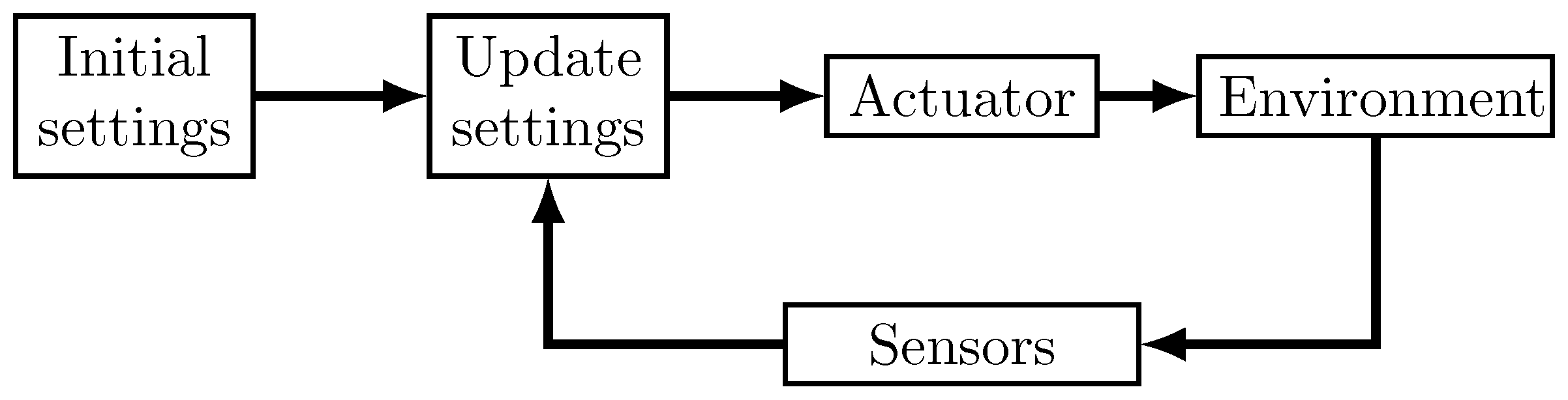
Figure 2.
Perceptron.
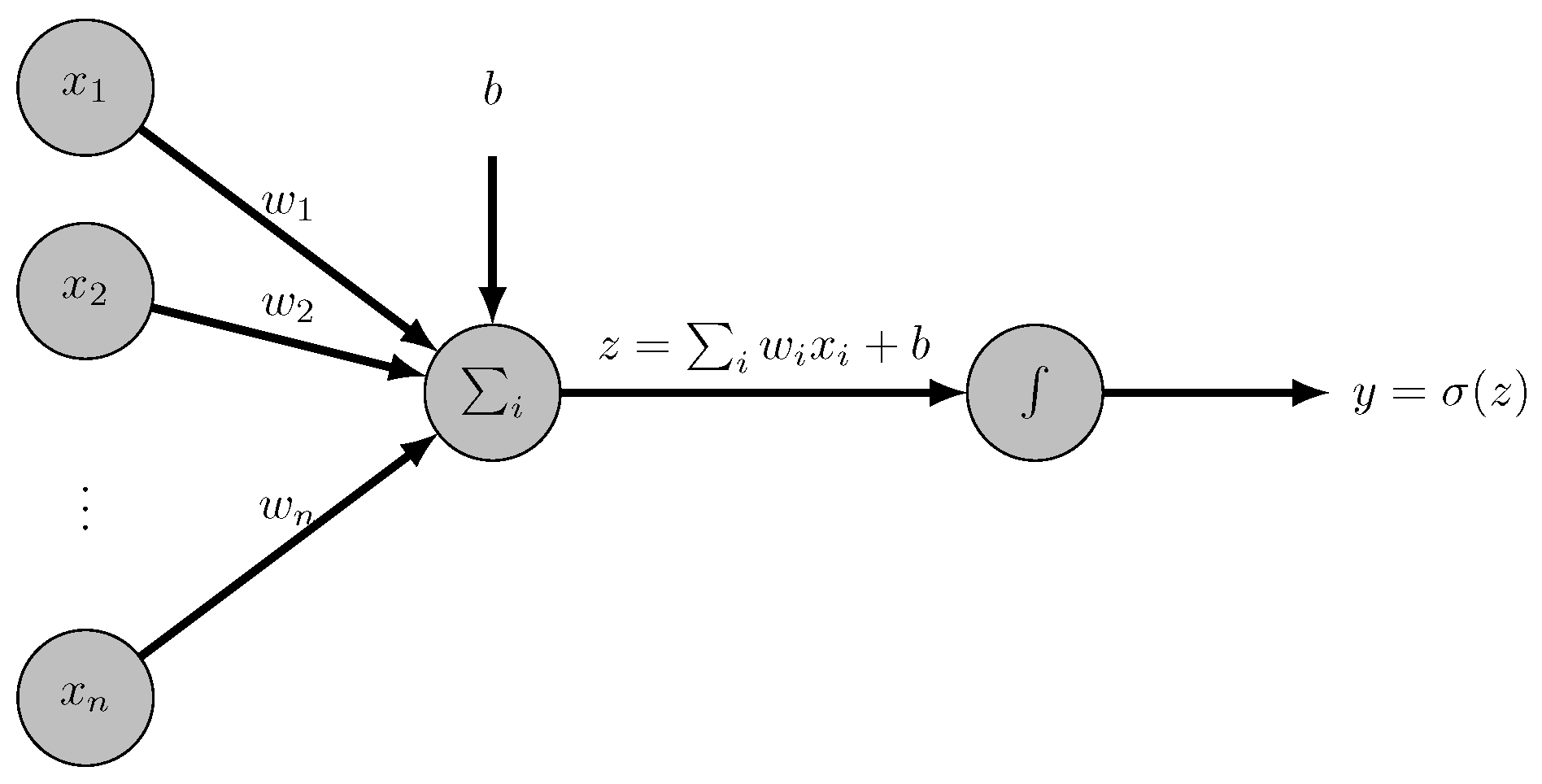
Figure 3.
Neural Network.
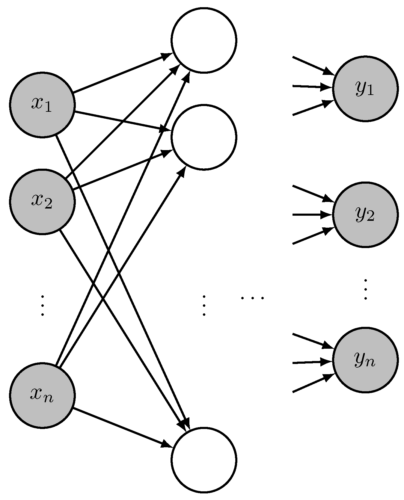
Figure 4.
Physics-Informed Neural Network.
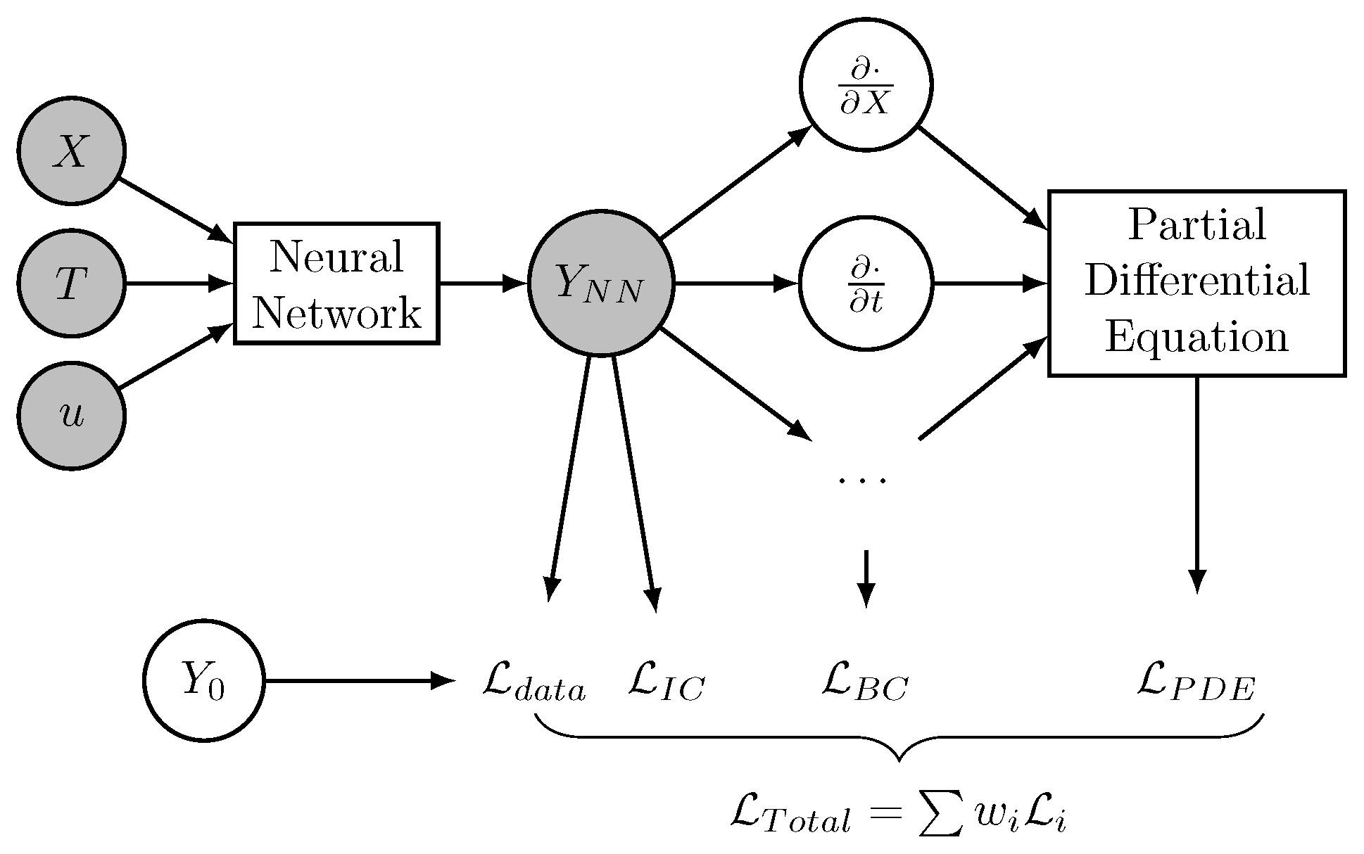
Figure 5.
Deep Q-learning training flowchart.
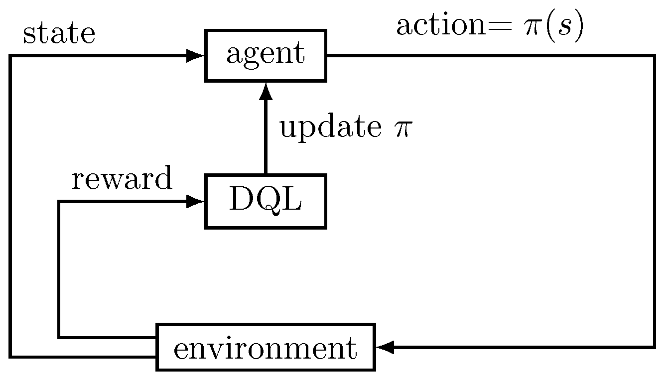
Figure 6.
1-dimensional bar as case of study.
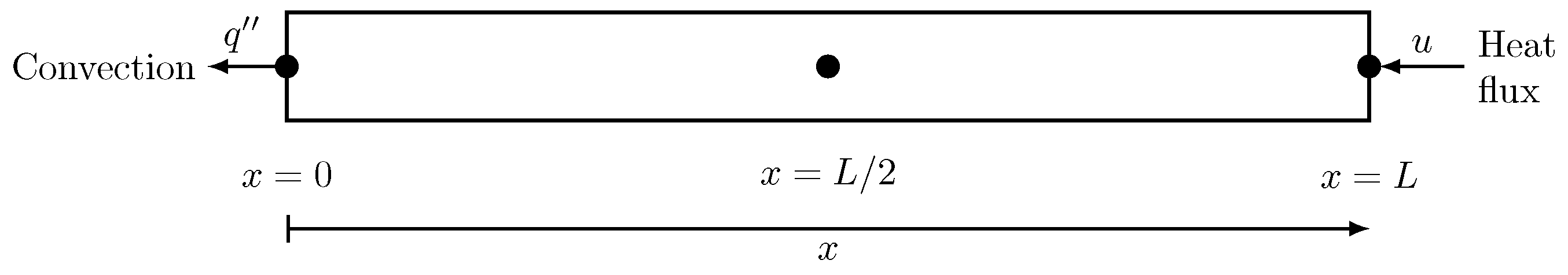
Figure 7.
Temperature distribution along time at three points: (red line), (green line) and (blue line), with no heating source.
Figure 7.
Temperature distribution along time at three points: (red line), (green line) and (blue line), with no heating source.
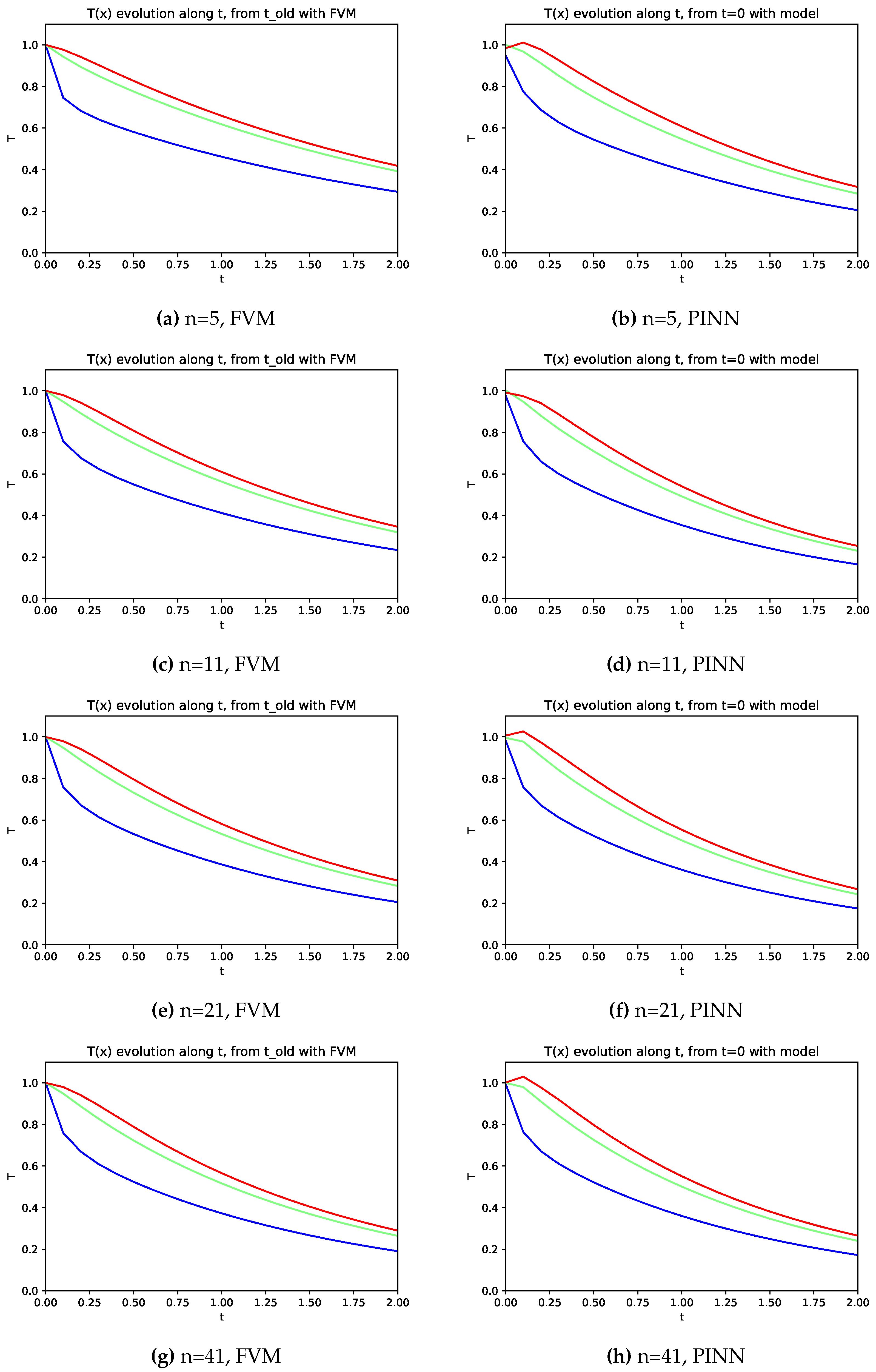
Figure 8.
Temperature distribution along x for (red line) up to (blue line), with no heating source.
Figure 8.
Temperature distribution along x for (red line) up to (blue line), with no heating source.
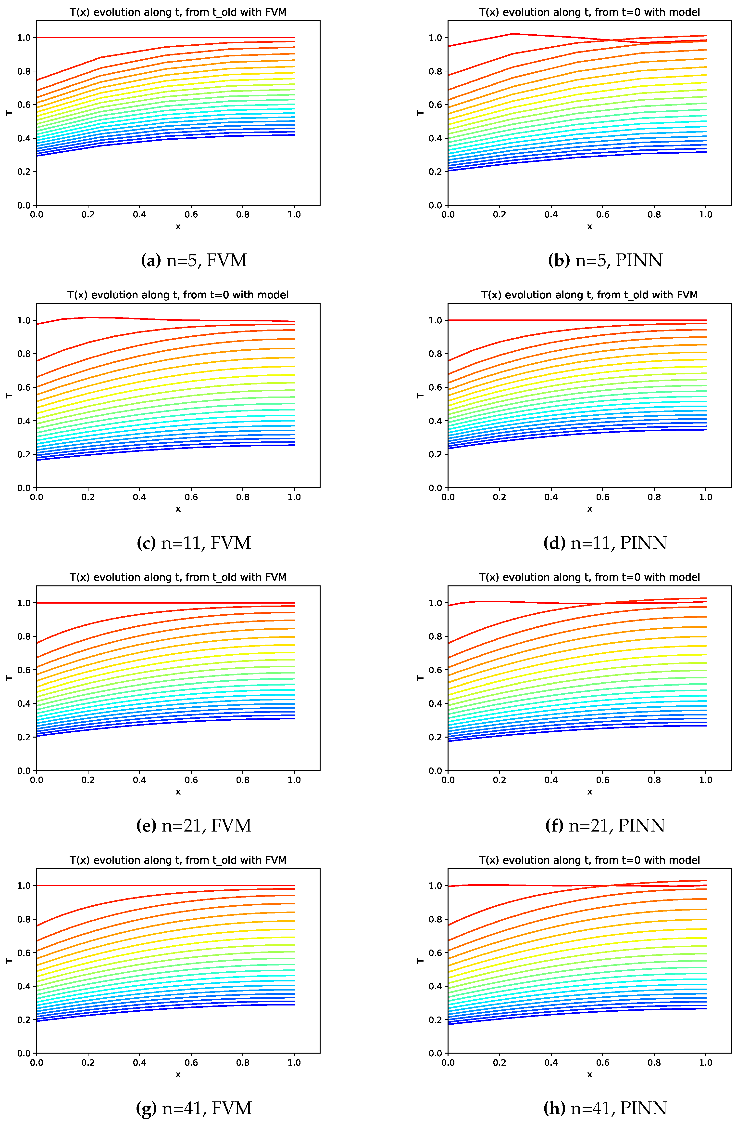
Figure 9.
Temperature distribution along time at three points: (red line), (green line) and (blue line), with bang-bang controller.
Figure 9.
Temperature distribution along time at three points: (red line), (green line) and (blue line), with bang-bang controller.
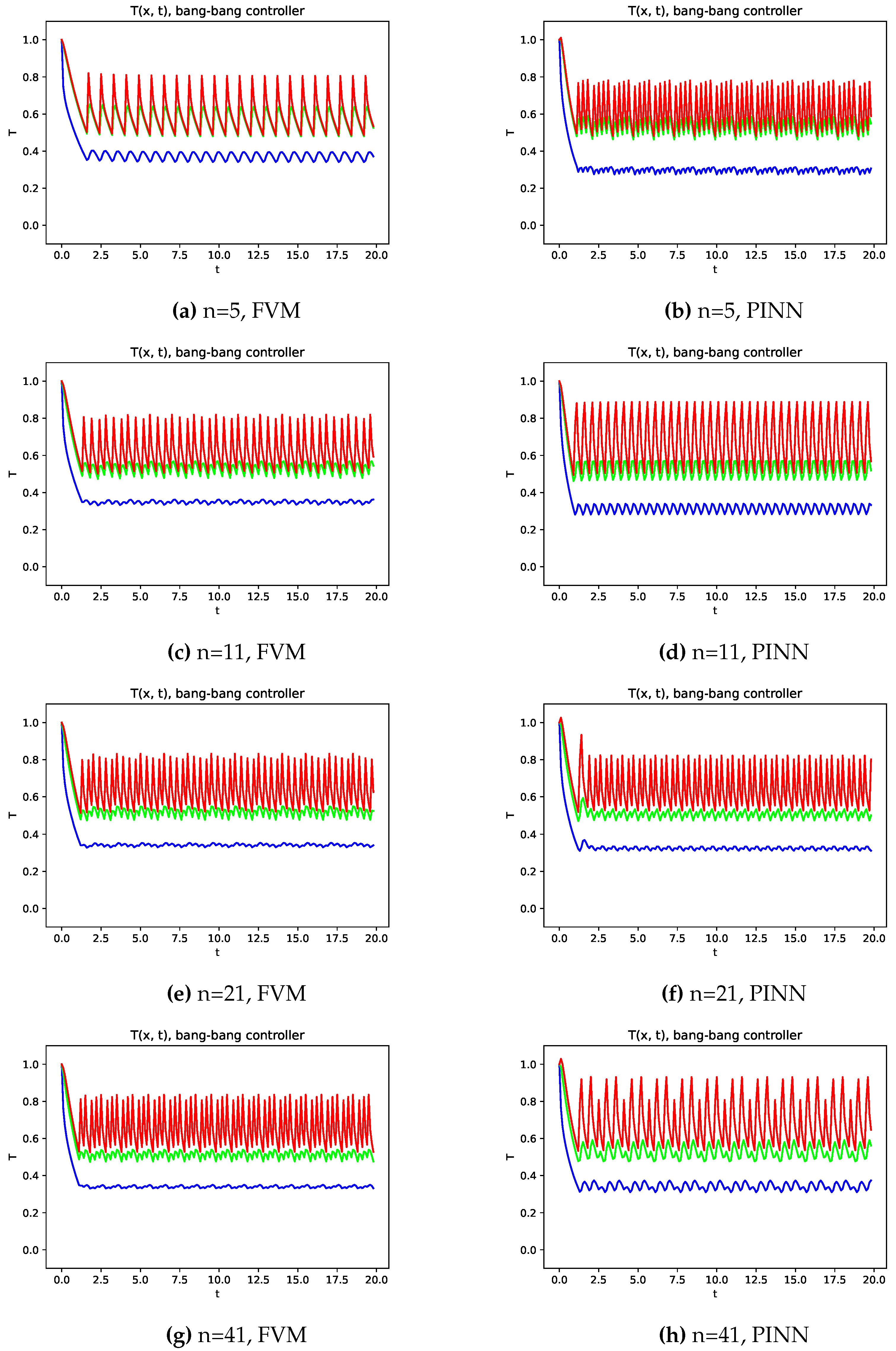
Figure 10.
Temperature distribution along time at three points: (red line), (green line) and (blue line), with DQL controller.
Figure 10.
Temperature distribution along time at three points: (red line), (green line) and (blue line), with DQL controller.
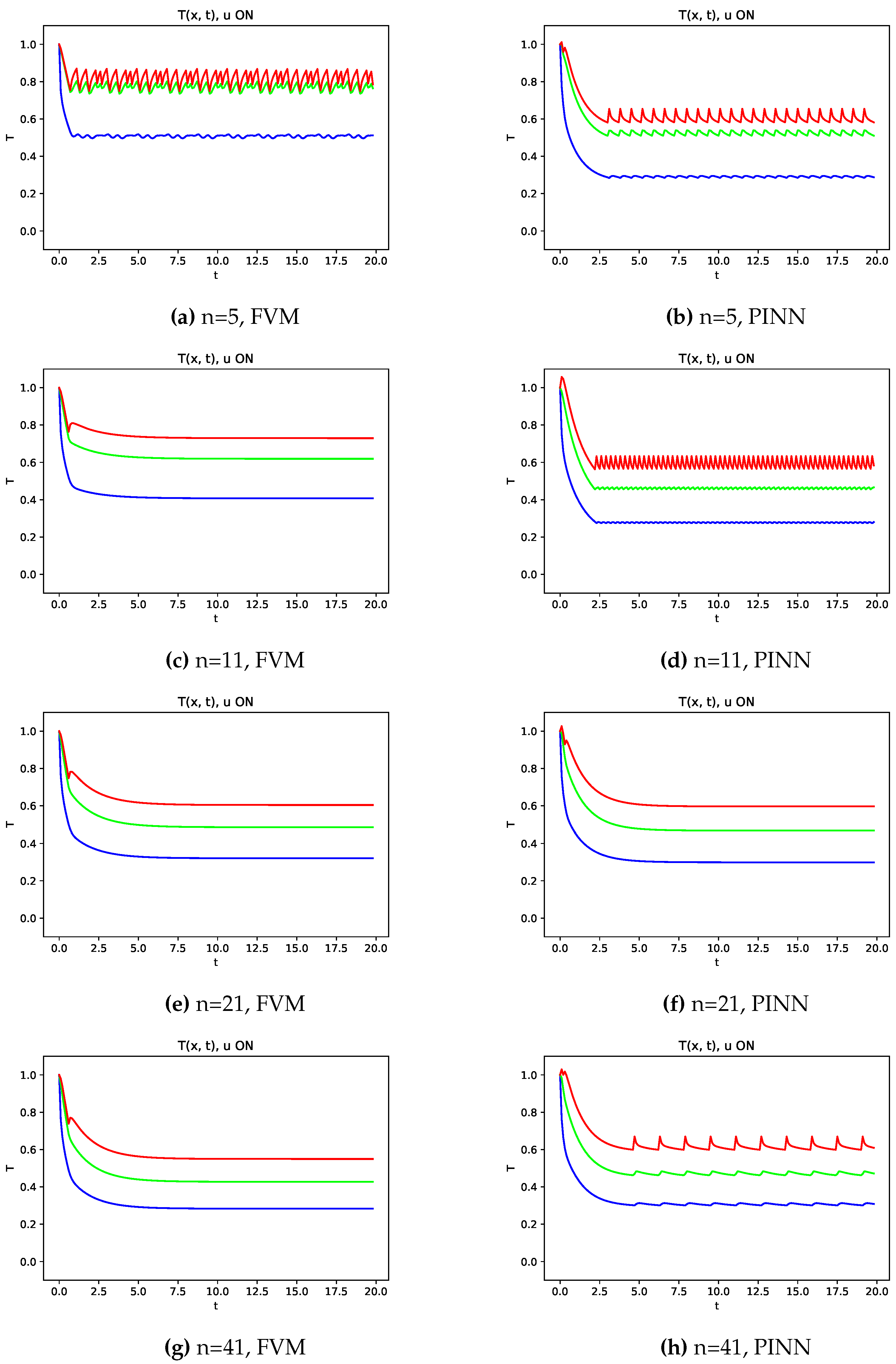
Figure 11.
Temperature evolution on the domain along the time, from initial stage (red line) up to final stage at (blue line) with Bang-bang control.
Figure 11.
Temperature evolution on the domain along the time, from initial stage (red line) up to final stage at (blue line) with Bang-bang control.
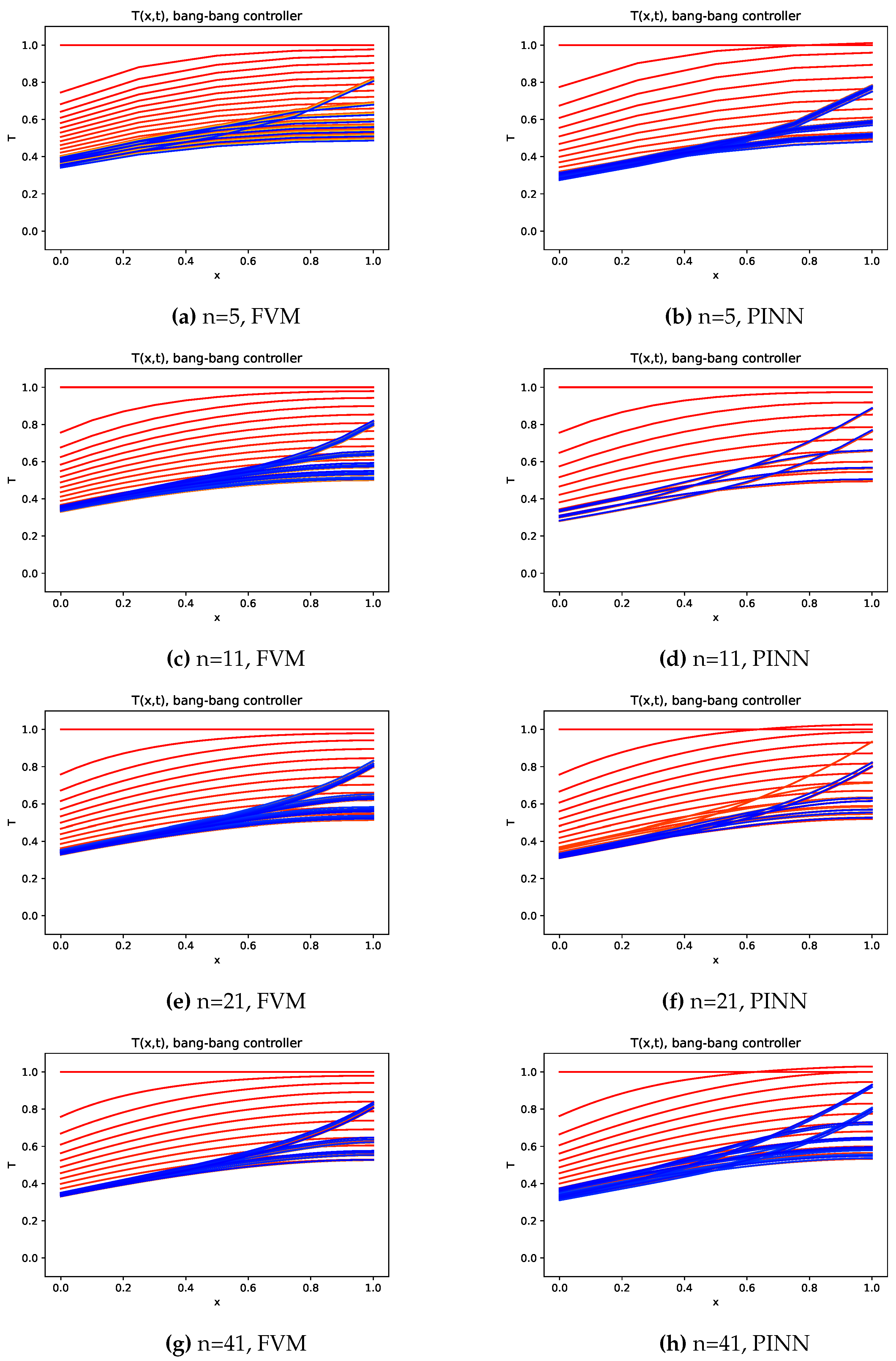
Figure 12.
Temperature evolution on the domain along the time, from initial stage (red line) up to final stage at (blue line) with model control.
Figure 12.
Temperature evolution on the domain along the time, from initial stage (red line) up to final stage at (blue line) with model control.
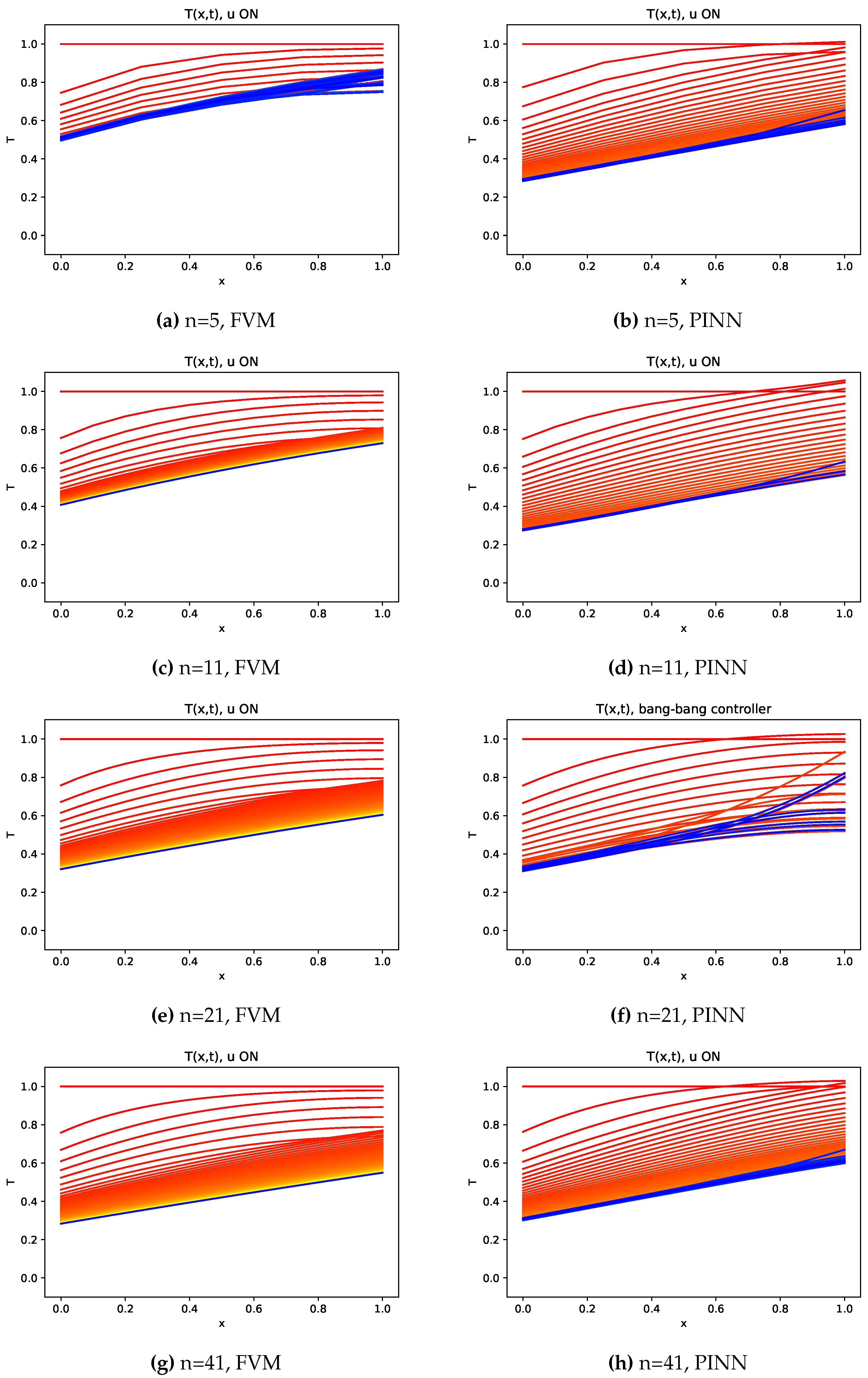
Figure 13.
Temperature at the control point obtained with progressivly finner meshes.
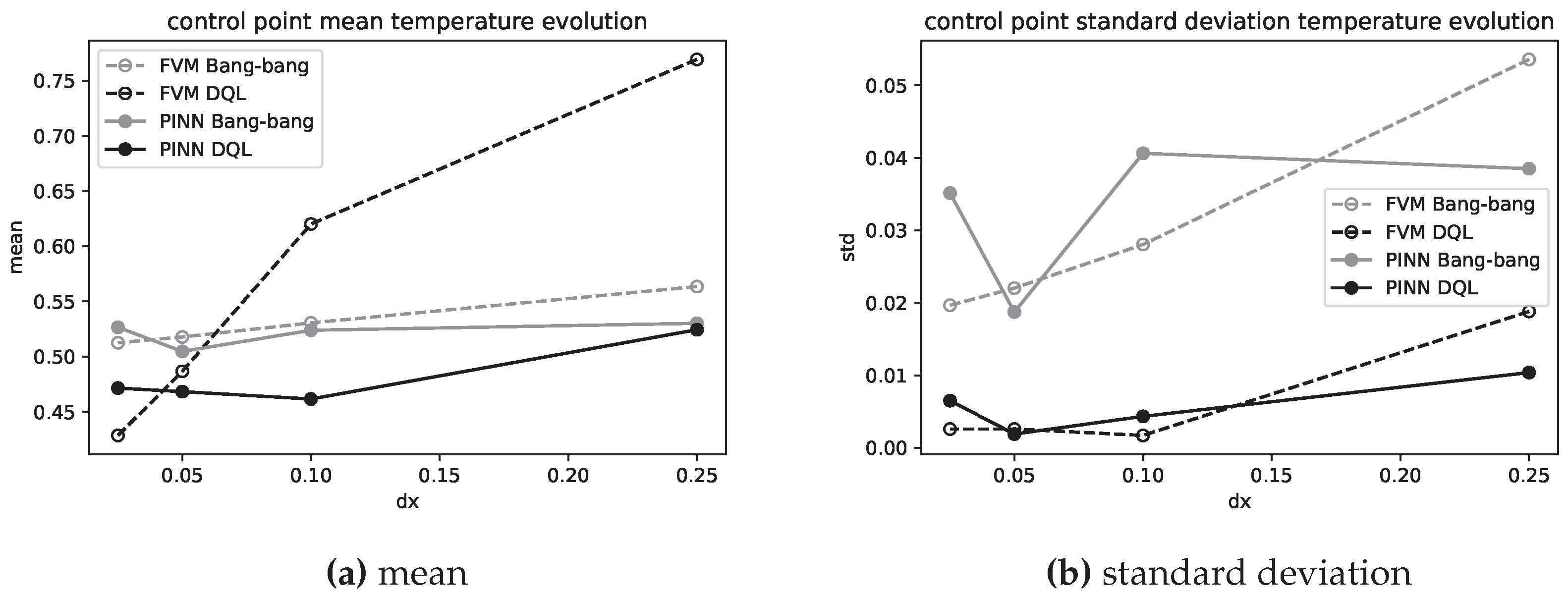

Table 1.
PINN algorithm.
| PINN algorithm |
|---|
| 1: set a set of initial conditions |
| 2: set training data intervals to consider |
| 3: define the Neural Network parameters: layers, nodes, and activation function. |
| 4: set learning parameters: learning rate, loss function |
| 5: train the Neural Network aiming to minimize loss function |
Table 2.
Deep Q-learning algorithm .
| DQL algorithm |
|---|
| 1: Initialize policy parameters |
| 2: |
| 3: for , do |
| 4: |
| 5: for , do |
| 6: Draw a random value |
| 7: if then |
| 8: choose a random action |
| 9: else: |
| 10: choose the action (available from the current state) that maximizes Q |
| 11: end if |
| 12: Execute the action and get a new state and reward (save on batch) |
| 13: if then |
| 14: train models |
| 15: update policy parameters |
| 17: end if |
| 18: if then |
| 19: |
| 20: end if |
| 21: end for |
| 22: end for |
Disclaimer/Publisher’s Note: The statements, opinions and data contained in all publications are solely those of the individual author(s) and contributor(s) and not of MDPI and/or the editor(s). MDPI and/or the editor(s) disclaim responsibility for any injury to people or property resulting from any ideas, methods, instructions or products referred to in the content. |
© 2024 by the authors. Licensee MDPI, Basel, Switzerland. This article is an open access article distributed under the terms and conditions of the Creative Commons Attribution (CC BY) license (http://creativecommons.org/licenses/by/4.0/).
Copyright: This open access article is published under a Creative Commons CC BY 4.0 license, which permit the free download, distribution, and reuse, provided that the author and preprint are cited in any reuse.


