
Submitted:
19 January 2025
Posted:
20 January 2025
You are already at the latest version
Abstract
This paper investigates the design and MATLAB/Simulink implementation of two intelligent neural reinforcement learning control algorithms based on deep learning neural network structures (RL DLNNs), in the case of a complex Heating Ventilation Air Conditioning (HVAC) centrifugal chiller system (CCS) selected as a case study. This system poses significant control-related challenges due to its high dimensionality and strong nonlinearity multi-input multi-output (MIMO) structure, coupled with strong constraints and a substantial impact of measured disturbance on tracking performance. As a beneficial vehicle for "proof of concept", two simplified CCS MIMO models were derived. At the same time, many simulations were run to demonstrate the effectiveness of both RL DLNN control algorithm implementations compared to two conventional control algorithms. Moreover, the experiments involving the two investigated data-driven advanced neural control algorithms prove their high potential to adapt to various types of nonlinearities, singularities, dimensions, disruptions, constraints, and uncertainties that inherently characterize real-world processes.
Keywords:
centrifugal chiller system
; reinforcement learning
; deep learning neural network
1. Introduction
Control algorithms are essential parts of the successful operation of processes. In recent years, data-driven intelligent control algorithms emerged as a valuable alternative to conventional model-based control methods. These algorithms mainly rely on artificial intelligence and soft computing concepts that make them highly efficient when controlling highly nonlinear, high-dimensional, time-delayed, time-varying, partially-known, or hard-to-mathematically-formalize systems. A special category of such new algorithms that employ the reinforcement learning principle to tune deep neural networks for optimal controlling of complex processes is still in the infancy stage but offers promising results. In this context, we aim to explore the development and Matlab/Simulink implementation of two neural reinforcement learning (RL) control algorithms that utilize deep learning neural network (DLNN) frameworks in relation to a specific intricate HVAC centrifugal chiller system, with the following four objectives:
To develop an accurate simplified multi-input multi-output (MIMO) Centrifugal Chiller System (CCS) model in a state space representation. Based on the input-output measurement dataset of the open loop MIMO CCS extended nonlinear model, having 39 states, three inputs and two outputs, a MIMO autoregressive moving average with an exogenous input (ARMAX) delayed polynomial model of fourth order in z-representation complex domain is obtained. Afterward, this ARMAX model is converted into a linearized MIMO CCS model with four states, three inputs, and two outputs.
- To design and tune a standard PID controller and also a standard model predictive control (MPC) for comparison purposes.
- To build two RL DLNN controllers connected in series in a forward path with the MIMO CCS simplified model in state-space representation for temperature control inside the evaporator subsystem and liquid refrigerant level control within the condenser subsystem.
- To rigorously analyze the tracking performance for both RL DLNNs and compare it with the one obtained using classic PID or MPC controllers.
The remainder of this research paper is structured in the following six sections. Section 2 is devoted to a brief literature review and some preliminaries regarding the considered HVAC system. Section 3 presents four traditional closed-loop control strategies, three of them derived from a standard PID controller, and the last one is an MPC designed and implemented in Matlab/Simulink, while Section 4 is devoted to the design of two RL DLNN controllers. The extensive simulation results are disseminated in Section 5. Section 6 is dedicated to discussions, while Section 7 concludes the paper, briefly highlighting the main yields and the future work directions.
2. Related Work and Preliminaries on HVAC Systems
2.1. Literature Review of HVAC Control Systems
It is well known that the electricity market is undergoing substantial transformations in grid modernization, large-scale energy storage and efficient energy transfer management. Many elements must work together to effectively provide the population and commercial consumers with the electricity services necessary for sustainable development. Both supply and demand will need to adapt to a new and diverse energy mix, including expanding demand-side management, building new energy storage capacities, and investing in modern and efficient power grids. In this context, a considerable amount of energy consumption in any commercial or residential building is due to heating, ventilation and air conditioning (HVAC) systems. Therefore, improving their efficiency becomes critical for energy and environmental sustainability. In general, centrifugal chillers are widely preferred cooling units for a wide range of HVAC control system applications for their high efficiency, reliability and low maintenance costs [1,2,3,4,5,6,7,8,9,10,11,12,13,14,15,16]. More precisely, they are suitable for providing cold water for the cooling needs of all the air-handling units in the building. Since a centrifugal chiller is the most energy-consuming HVAC device, its efficiency can be improved by using advanced model-based as well as data-driven controller design strategies [14,15,16,17,18,19,20,21,22,23,24,25,26,27,28,29,30,31,32,33,34,35,36,37,38,39,40,41,42,43,44]. A brief review of the HVAC centrifugal chiller literature reveals that a significant amount of work has been done on steady-state and transient modeling. Several dynamic models for the vapor compression cycle have been extensively studied [6]. Also, in [1,2] a mechanistic, single stage and two-stage centrifugal chiller models are developed for which the centrifugal compressor is modeled based on the Euler turbo-machinery, the balance energy and the impeller velocity equations. The energy coefficient of performance (COP) of the chiller is simulated by considering the compressor polytropic efficiency, and hydrodynamic, mechanical and electrical losses. On the other hand, the condenser and evaporator are modeled based on the lumped parameter approach, and the heat transfer is calculated based on the effectiveness model [14]. Taking into account the fact that their dynamics are of high nonlinearity, complexity, and dimensionality, from an appropriate control perspective, the developed models must be simplified as is done in [14,15,16]. An interesting dynamic model of a semi-hermetic reciprocating compressor is developed based on the first law of thermodynamics applied to a lumped control volume, the expansion valve modeled based on a simple orifice flow model [1,2]. Over the past two decades, our research team has worked intensively in HVAC field control systems, focusing on developing high-fidelity dynamic modeling of centrifugal chillers and building the most suitable control strategies based on them, as a priority task of our research [14,15,16]. Interested readers and specialists working in the field can find valuable support in developing simplified, linearized, low-dimensionality, accurate, robust, and stable models in different state-space representations or in the complex domain. Moreover, these models are validated and adapted to an harshment realistic working environment reached in a variety of uncertainties, nonlinearities, high dimensionality, and disturbances. Therefore, this paper presents some models of multi-input-multi-output (MIMO) centrifugal cooling systems (CCS) with enough details for good readability and understanding. Based on these, some advanced closed-loop intelligent neural control strategies of real practical interest are developed. More specifically, these models are chosen for our case study as a valuable vehicle for "proof of concept" and simulation purposes. These models are inspired by the field of literature, one of the works being fundamental as the one mentioned in [17], and those mentioned in [18,19,20,21,22,23,24] are some valuable and useful references for the design of models based on discrete-time data, such as AutoRegressive with eXogenous input (ARX) and Autoregressive Moving Average with eXogenous input (ARMAX), polynomial models built in a state space. Compared to standard control strategies, such as the Proportional Integral Derivative (PID) control and also Model Predictive Control (MPC), the advanced neural intelligent reinforcement learning Deep Learning Neural Network (RL DLNN) control systems surpass in various abilities such as possessing human-like expertise in a particular domain, self-adjusting and adaptively learning environmental changes and taking the best decisions or most appropriate actions [25,26,27,28,29,30,31,32,33,34,35,36,37,38,39].
2.2. Preliminaries – Adopted CCS Model and Its Implementation
This research uses a valuable vehicle, namely three MIMO Centrifugal Chiller System (CCS) models, adopted as a case study, for “proof of concept” and MATLAB simulation purposes.
2.2.1. MIMO Centrifugal Chiller Modelling Assumptions
The proposed MIMO (three inputs, two outputs) centrifugal chiller model used in the case study for this research is developed with sufficient details in [15, Annex 1,pp.299-305] and also validated in [14]. In this research, the model is simplified to be suitable for control purposes based on the aforementioned model. In the case study the proposed dynamic model of the Centrifugal Chiller system is built by interconnecting the following subsystems: water-cooled centrifugal chiller, a centrifugal compressor, shell-and tube heat exchangers, a thermal expansion valve, and the controller. The water-cooled centrifugal chiller is modeled based on the mechanics of fluid theory, as well as the centrifugal compressor that is modeled based on the turbo-machinery theory, similar to those developed in [14,15]. The chiller capacity control is achieved by the combination of variable inlet guide vane and variable speed drive and the entire system consists of four major components [1,2,14,15,16], as is shown in Figure 1, namely a centrifugal compressor,a condenser,an expansion valve, and an evaporator. In general, the overall chilled-water system consists of one circuiting refrigerant loop and two water loops. The first water loop is circuited between the condenser and the cooling tower, and the second water loop is circuited between the evaporator and the air handling units (AHU) that produces chilled-water for the cooling coil.
A thermal expansion valve is used to regulate the pressure levels at the condenser and evaporator sides. In this research the overall dynamics of the MIMO chiller control system in a state-space representation by a set of 39 nonlinear differential equations, thus with 39 states, two inputs (compressor driver relative speed ( ), expansion valve opening (%) ), and two outputs (water temperature, liquid level in the evaporator). The impact of load temperature, as a main disturbance is under investigation also. Even if the centrifugal chiller is highly dimensional system, it could be easily integrated to various control HVAC control applications of commercial buildings, the chilled-water system supplying chilled-water for the cooling needs of all the building’s air-handling units. In order to accomplish these tasks HVAC control systems include mostly a water pump to circulate the chilled water through the evaporator and throughout the building for cooling. Also, another water loop from the chiller rejects heat to the condenser water, where another pump circulates the heated water to the cooling tower and cooled back [11,14,15,16]. The main goal of this research is to improve the existing works towards comprehensive dynamic models for the whole chiller to achieve a performance of high accuracy in an attractive MATLAB and Simulink modeling and simulation environment for all components of centrifugal chiller. The closed-loop control strategies centrifugal chiller model-based and data-driven developed in the following sections seems to achieve the best transient and steady-state performance.
2.2.2. Case Study – MIMO Centrifugal Chiller System Assumptions and Decompozition
The dynamic model of the overall centrifugal chiller control system is of high complexity in terms of state dimensionality and nonlinearity and is described in state-space by a set of 39 first order differential equations (ODE), as a natural mathematical form to represent a physical system. It is beyond our purpose to write now all these equations, since a MIMO centrifugal chiller model used in the case study is already developed and validated with sufficient details in [14, 15 |Annex 1,pp.299-305] but some significant aspects in a modeling methodology we will present briefly in this section. The first assumption under consideration in the case study is related to decomposition of the overal Centrifugal Chilller control system in two embedded open-loop subsystems, the first one is an open-loop Temperature control of the chilled water Tchw_sp, inside Evaporator subsystem, and th second one is an open-loop Level control of the liquid refrigerant level L, inside Refrigerator subsystem. Second assumption is related to the interference and independence of both loops. Based on two of these assumptions, three inputs and two outputs MIMO model with Temperature load disturbance, two independent loops can be attached to a data-based CCS model to be investigated, more precisely the input triplet (Compressor speed Ucom, Expansion valve opening U_EXV, Temperature load disturbance Tchw_rr (chilled water return temperature)) and an output doublet (Temperature Tchw_sp , Level L). It is worth noting that this modelling strategy, using a deterministic input disturbance Tchw_rr, is the most realistic in real life which is of particular interest to be investigated. As oriented object, the MIMO Centrifugal Chiller plant, in MATLAB is considered as an iddata object, generated based on the input-output measurements dataset loaded in MATLAB workspace using the following MATLAB code lines:
- load InputOutputChiller_Data.mat Tchw_sp Level Ucom U_EXV Tchw_rr;
- CentrChiller = iddata (y,u,1)
- where the input-output measurements dataset is collected in open-loop using a specific data acquisition equipment and strored in the input vector u=[u1 u2 u3] which is a three columns vector assigned to:
- u1= Ucom; u2 = U_EXV; u3 = Tchw_rr, and in the output vector y=[y1 y2] that is a two columns vector assigned to:
- y1 = Tchw_sp for Chilled water Temperature inside the Evaporator subsystem
- y2 = Level for Liquid refrigerant level of the Refrigerator subsystem
2.2.3. Open Loop MIMO Centrifugal Chiller System (MIMO) –MATLAB Simulink Extended Model Diagram
The MIMO Centrifugal Chiller System dynamics is represented in state space by a MIMO Simulink model with three inputs (u1=Ucom, u2=U_EXV, u3=Tchw_rr), two outputs (y1 = Tchw_sp, y2 = Level) and 39 states described by 39 nonlinear first order differential equations encapsulated in a MATLAB function block as is shown in Figure 2.
Figure 2.
Simulink model of MIMO Centrifugal Chiller System in state space representation.
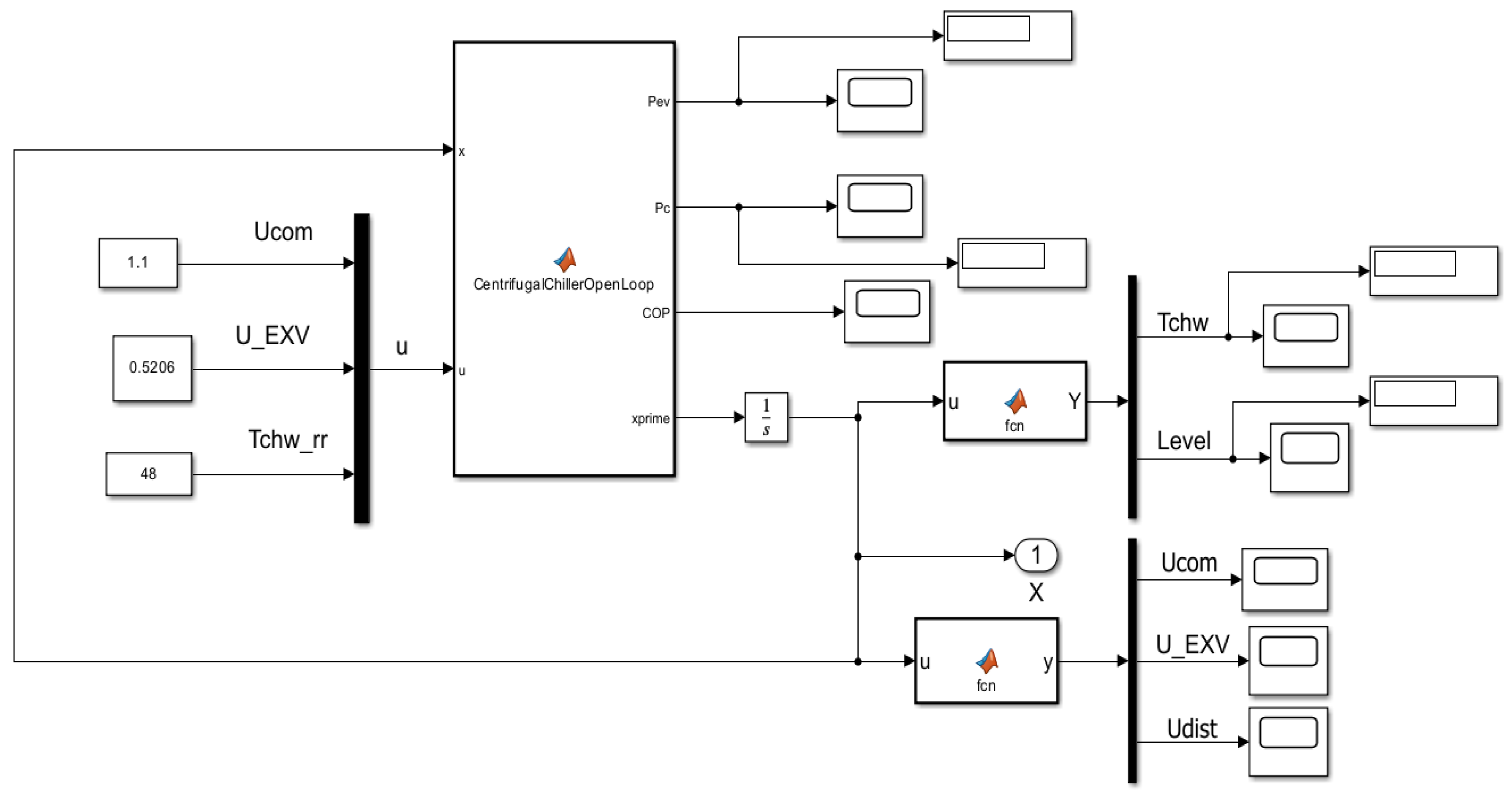
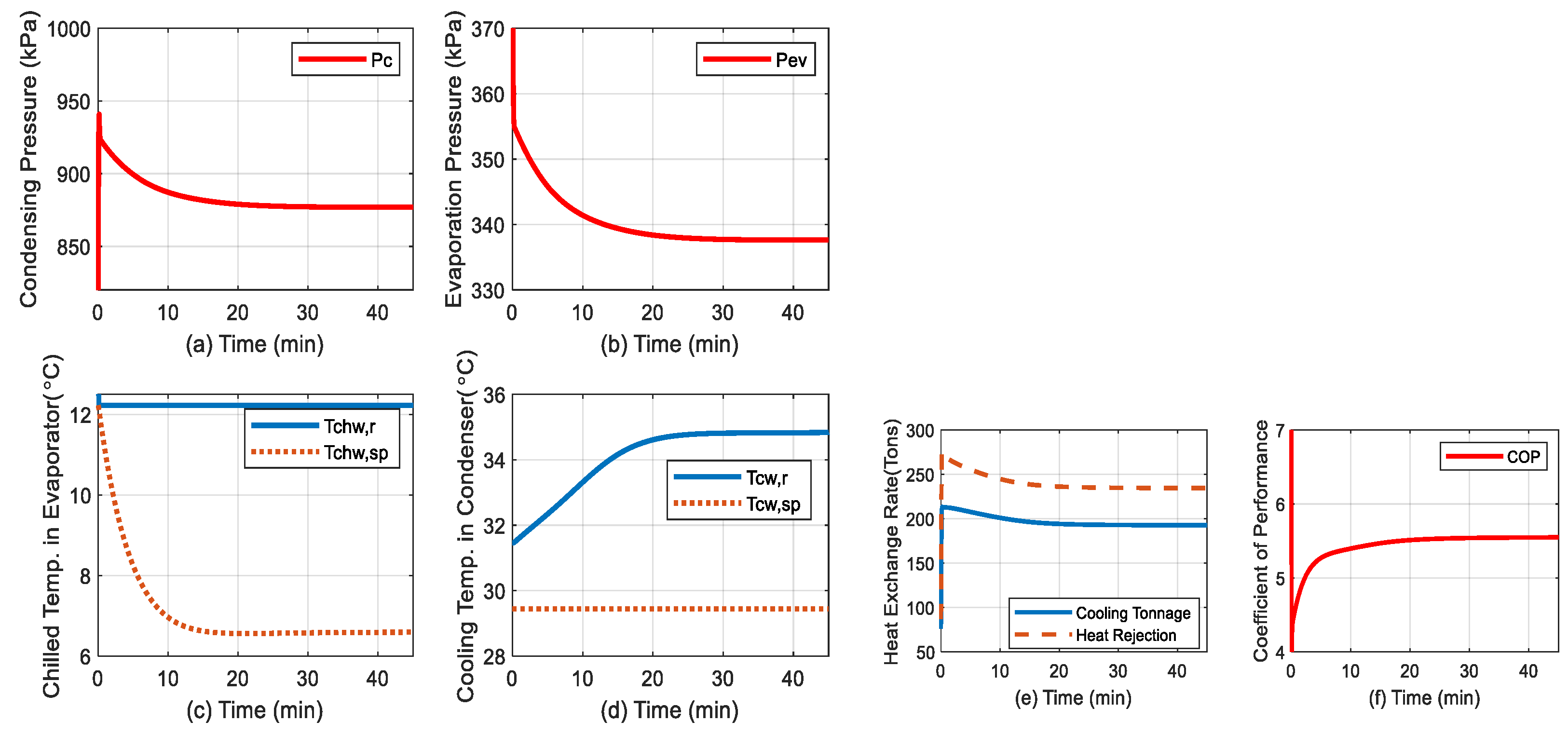
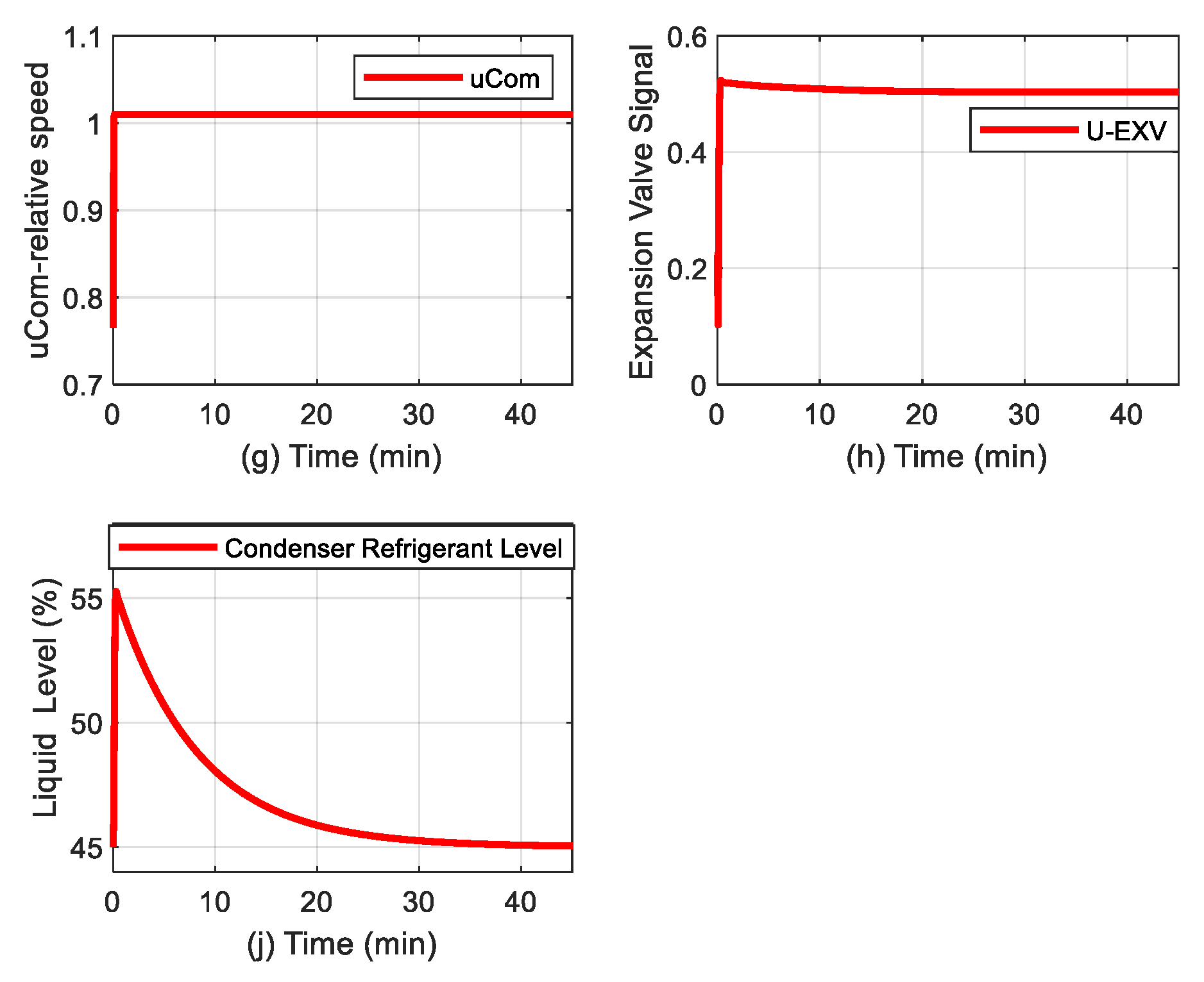
Figure 3.
MATLAB Simulink open-loop simulation results. (a) Condensing Pressure (Pc); (b) Evaporator Pressure (Pev); (c) chilled water temperature (Tchwr) in Evaporator; (d)cooling water temperature (Tchwsp) in Condenser; (e) heat exchange rate; (f) coefficient of Performance (COP); (g) uCom input – relative compressor speed (RPM/RPMnominal);(h) u_EXV input-expension Valve opening in (%);(i) the liquid refrigerant level in Condenser (%);(j) The MATLAB function selected for visualization Block.
2.2.4. Case Study -The Data-Driven ARMAX Model for MIMO Centrifugal Chiller Subsystems in Discrete-Time State-Space Representation
The MATLAB System Identification Toolbox provides valuable tools to develop second order polynomial ARMAX simplified model of high accuracy assigned to MIMO Centrifugal Chiller full model. This simplified model is very useful to build two traditional closed loop control strategies, namely a PID and MPC, as well as two alternaive advanced intelligent reinforcement learning control strategies based on the Reinforcement Learning Deep Learning Neural Networks (RL DLNN) as a viable alternative to both traditional ones. Finally, a rigurous performance analysis will be made for comparison purpose, in order to decide which one perform much better in terms of meeting the control design requirements and process control constraints, rejection the effect of possible disturbances that act on the controlled process, as well as a tracking error accuracy. The original MIMO ARMAX model is developed in state-space representation, by a nonlinear set of ordinary differential equations (ODE), as a natural representation of a physical system, and easily to be solved using a suitable MATLAB solver. This MIMO Centrifugal Chiller nonlinear model of high dimensionality (39 states) is simplified and also described in a state-space representation.
The following two MATLAB code lines generate the MIMO ARMAX (MIMO) discrete state-space model in z-complex domain [7,34]:
where the options are selected by using the MATLAB code line:
MIMO =armax(CentrifugalChiller_DATA, [[2 0; 0 2],[2 2 2; 3 2 3], [1; 1], [1 1 1; 1 1 1]], options)
options = armaxOptions(‘InitialCondition’,’estimate’,’Focus’,’prediction’)
In z-complex domain, the MIMO ARMAX Centrifugal Chiller model generated in MATLAB is a three inputs, two outputs and four states linear model described in discrete time state space by a triplet of matrices (A, B, C) given by [15,16,17,18,19,20,21,22,23,24,32]:
or compact in a discrete-time z-transform transfer matrix representation:
such that:
where for each input-output chanel correspond the following z-transfer functions:
From the channel input "u1" to output “y1”the discrete-time transfer function is given by:
From the channel input "u1" to output “y2”the discrete-time transfer function is denoted by:
From the channel input "u2" to output “y1”the discrete-time transfer function is represented by:
From the channel input "u2" to output “y2”the discrete-time transfer function is designated by:
From the channel input "u3" to output “y1”the discrete-time transfer function is given bellow:
From the channel input "u3" to output “y2”the discrete-time transfer function is defined as:
The Simulink diagram of MIMO centrifugal chiller model in z-domain including all these z-transfer functions is represented in Figure A1 from Appendix A.
A compact matrix description of MIMO ARMAX Centrifugal Chiller System in discrete-time state space (three inputs, 4 states, two outputs and a sampling time, Ts = 1 second, is given by the following state space equation
with the values of the matrices quadruplet (A, B,C and D) coefficients given in Eq.(7).
The MIMO output responses, the disturbance temperature set to Tchw_rr = 48 [°F ] and actuators inputs (Speedcomp, ExpValve) are shown in Figure 4.
3. Traditional Controllers-PID and MPC Closed Loop Control Strategies
In the time domain, the general form of PID control law in a closed loop control strategy is given by the following input-output equation:
where represents the error between the actual measurement of system output and its desired value , called also setpoint, referrence or tracking value:
is designated for controller output
represent the PID controller parameters, -is the proportional gain, -designates the integral gain, - denotes the derivative gain, and and are the time constants for integral and derivative blocks, respectively. For a particular parameters setting can be obtained different controller architectures, such as P, I, PI, PD and PID.
In complex domain, the transfer function of the PID controller is given by
corresponding to an ideal PID controller. Furthermore, adding a compensator formula to Eq.(10) using a Low Pass Filter (LPF) of coefficient N is otained a practical PID controller, of the following transfer function
3.1. DTI MIMO Centrifugal Chiller Closed Loop System Control in State Space Representation
The Discrete Time Integrator (DTI) closed loop control strategy architecture of the proposed MIMO CCS model as a valuable “vehicle” for MATLAB Simulink simulations is depicted in Figure A2 from Appendix A. Its discrete time transfer function in z-complex domain is given by
The parameters of both DTI controllers blocks are much easier to adjust, instead a PID controller due to constraints subjected the inputs, , the adjustement parameters encounters some difficulties. Also, a "trial and error" procedure to track evaporator temperature and condenser level performance is inaccurate. In the Figure A2a is represented the compact DTI Simulink diagram with valuable details for both integrators shown in Figure A2b and Figure A2c.
3.2. PID MIMO Centrifugal Chiller Closed Loop System Control in Extended State Space Representation
The PID closed loop control strategy for MIMO Centrifugal Chiller System (CCS) extended model with 39 internal states is depicted in Figure A3a-c. The PID transfer function in s-complex domain is given by Eq.(11). The both controllers parameters dataset for Evaporator Temperature (indexed by T) and for Condenser liquid Refrigerant Level (indexed by L) are set to the following values:
, the temperature setpoint within Evaporator is Tchw_sp = 6.67 [degC], and the liquid Refrigerant Level inside Condenser is L = 45 (%) , and a much longer simulation time of Tf = 13600 seconds (3 hours 30 minutes).
Therefore, alternative simplified ARMAX, ANFIS and neural network models of the MIMO Centrifugal Chillaer capable of capturing its entire dynamic evolution and suitable for the control purpose are investigated in this research.
In Figure A3a is shown the Simulink diagram of PID closed-loop control strategy, and in Figure A3b is presented two subsystems components of the Simulink diagram (model + visualization block). The code lines of the Simulink MATLAB function from visualization block are given in Figure A3c. The Simulink simulations result is depicted in Section 5, and a rigurous performance analysis is done in Section 6.
3.3. Digital PID Control of MIMO Centrifugal Chiller Closed Loop System in Extended State Space Representation (39 States)
A large number of simulations performed on a MATLAB Simulink R2024a platform reveal a slow response of about 3 hours and 30 minutes to reach a steady state and achieve accurate tracking performance for the Evaporator subsystem Temperature and liquid Refrigerant of agent Level control in the Condenser subsystem. A substantial improvement is the development of a fast-tuning digital PID controller, similar to an interesting approach proposed in [35]. Furthermore, an alternative to the extended MIMO centrifugal chiller model, a simplified Adaptive Neural Fuzzy Inference System (ANFIS) is under investigation to be integrated with the digital PID in the same closed-loop control strategy, whose diagram Simulink block is shown in Figure 5. MATLAB Simulink simulations are disseminated in Section 5 and a rigorous performance analysis is done in Section 6, revealing a fast response. (settling time) and high tracking accuracy. Moreover, this performance is compared with an advanced deep learning neural network (RL DLNN), for which the reward function is generated based on the step response block specifications of a digital PID control of a MIMO CCS ANFIS model, developed in the next section.
In the Simulink diagram shown in Figure 8, the digital PID controller appears in the left side, implemented based on Eq.(8). The simplest way to implement a digital PID is to discretize Eq.(8) and then to transform it in a difference equation, of the following form, suggested in [44]. More specifically, it is a recursive method that calculates the PID controller output at based on the previous value of the controller output and its growth [44]:
For simplicity, assuming , Eq.(13) becomes:
or compact,
with the coefficients given by:
In this research the controller coefficients are set to (0.095, -0.225, 0.1) for the first digital PID controller integrated into a closed-loop feedback control of the chilled water temperature inside the Evaporator subsystem, ANFIS model.
The second set of values (0.025,-0.105,0.05) is selected for the second digital PID controller that controls the liquid refrigerant level in the Condenser subsystem, ANFIS model. If you can see, the MIMO Centrifugal model is split into two accurate ANFIS models of the MIMO centrifugal chiller, the first is a MISO ANFIS CentrChillerfis1 attached to the Evaporator subsystem and the second one is a MISO ANFIS CentrChillerfis2 assigned to the Condenser, as shown in Figure 6a-h. Both MISO ANFIS models are generated using Fuzzy Logic Designer app based on the measurement input- output dataset of the open loop MIMO Centrifugal Chiller plant. The first ANFIS MISO Evaporator Centrifugal Chiller model (fisCentrChiller1) is shown along with the membership functions in Figure 6a-b and its estimation performance in Figure 6e. The second ANFIS MISO Condenser centrifugal chiller is exposed along with the membership functions in Figure 6c-d and its estimation performance in Figure 6f. The Figure 6g-h shows a Rule Viewer for each MISO ANFIS model.
3.4. Model Predictive Control Based on Centrifugal Chiller MIMO State Space Representation
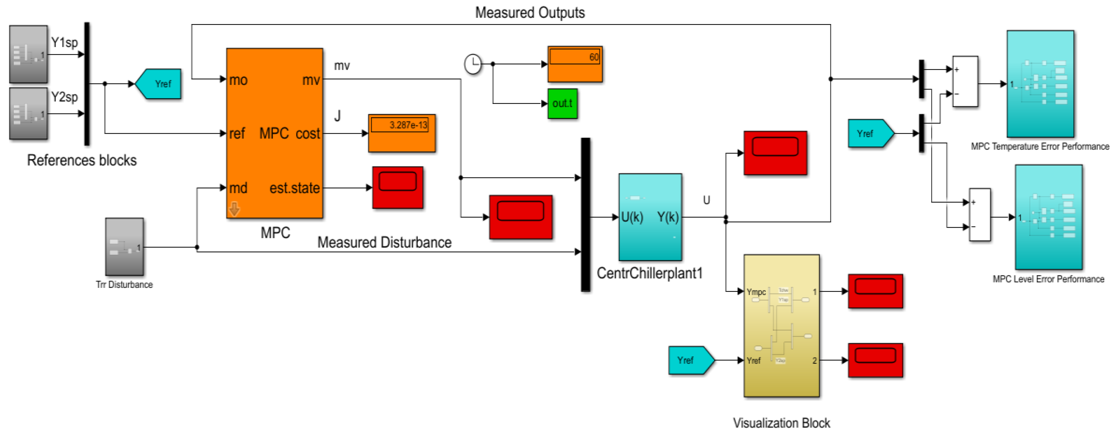
The MPC closed-loop control strategy architecture for MIMO CCS is shown in Figure 7. The Model Predictive Control (MPC) object is generated in MATLAB as is explained with enough details in Section 4.2, and the MPC Simulink diagram block shown in Figure 7 is provided from MPC MATLAB Simulink Toolbox. The MPC object has two manipulated variables (MV) uCom and u_EXV, one measured disturbance (MD) (temperature Trr set to 48 degree Fahrenheit) and two measured outputs variables (OV), namely Evaporator Temperature Tchw_sp and liquid Refrigerant Level inside Condenser. The MIMO model of the Centrifugal Chiller plant is represented in a discrete time state space by Eq.(6) with the values of the matrices’ coefficients given in Eq.(7). The MATLAB Simulink simulations results are shown in Section 5.2 and the performance analysis in Section 6.
Figure 7.
The Simulink models of MPC using Simulink MPC Toolbox and mpcDesign application.
4. Design and Implementation of Reinforcement Learning Using Deep Learning Neural Networks-MIMO CCS Closed Loop Control Strategies
This section is focused on the design and implementation in MATLAB Simulink of two RL DLNN advanced intelligent control strategies for MIMO CCS simplified state space model, first one is using an MPC specifications to generate the reward function, and the second one using the step response specifications imposed to an MIMO CCS model represented in a simplified state space. The tracking accuracy performance is compared to MPC integrated in the first controller structure, and an improved digital PID based on MISO CCS ANFIS models.
4.1. Reinforcement Learning Closed Loop Control Strategy using Deep Learning Neural Networks MIMO Centrifugal Chiller Plant Model Based Represented in State Space Representation
Reinforcement Learning (RL) is a process in which an agent (controller) learns to make decisions interacting with an uknown environment through trial and error, as is shown in Figure 8a [37,38]. Mathematically, the modelling RL process (algorithm) depicted in Figure 8a is typically based on a Markov Decision Process (MDP), where the RL agent block at every timestep receives an observation by interacting with an unknown Environment in a current state St and takes an action At sent to same Environment that reacts by sending a scalar reward Rt. Then RL block receives the reward signal and transitions to the next state St+1 according to Environment dynamics conditional probability p(St+1|St, At). The RL agent attempts to learn a policy π(At|St), or map from observations to actions, in order to maximize its returns (expected sum of rewards). In RL (as opposed to optimal control) the algorithm only has access to the dynamics p(St+1|St, At) through a sampling time. A comprehensive definition of the RL algorithm, widespread for control and planning applications, can be found in [37] which states that “Reinforcement learning is a goal-directed computational approach where a computer learns to perform a task by interacting with an unknown dynamic environment”. During the training process to learn the unknown environment “enables the computer to make a series of decisions to maximize the cumulative reward for the task without human intervention and without being explicitly programmed to achieve the task” [37].
Figure 8.
Reinforcement learning architecture (reproduced from [37,38]); (a) RL process; (b)Standard feedback closed loop control schematic.
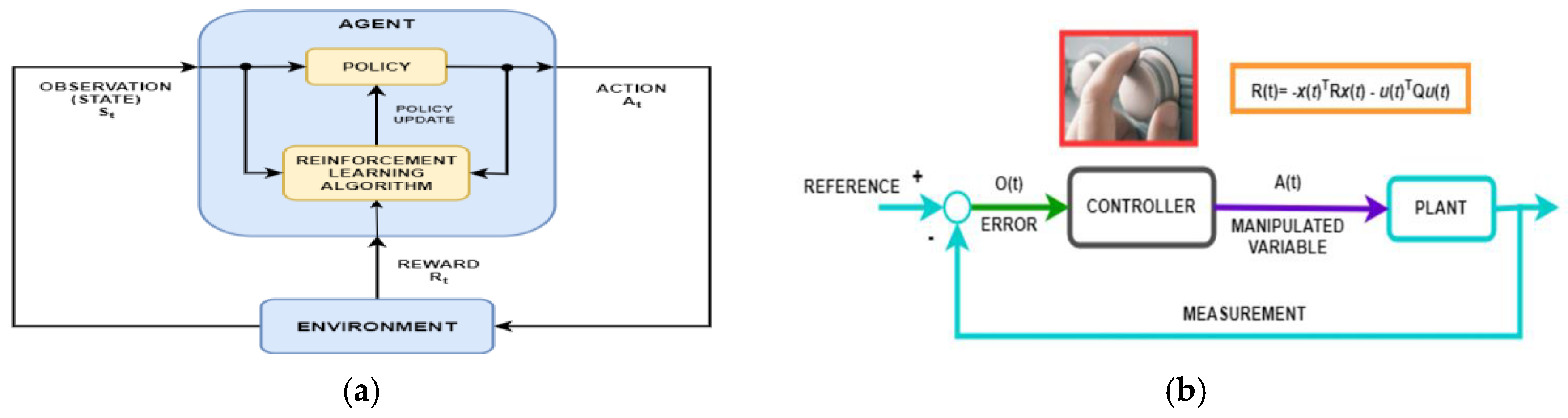
From the perspective of a system-oriented approach, the diagram shown in Figure 8a shows a general representation of a reinforcement learning (RL) algorithm, and Figure 8b mostly exposes its equivalence to a traditional loop control strategy closed. used in system applications [38]. In other words, the key role of the RL policy in Figure 8a is to observe the unknown environment (state St) and generate actions (At) to “complete a task optimally”, so similar to a controller traditionally operating in a control system application. Of course, the RL algorithm comes with a valuable improvement to the RL policy, known as policy updating. More specifically, RL can be seen as a mapping of a traditional feedback control system depicted in Figure 8b, and the correspondence between both diagrams is well presented in [38]. The agent receives observations and a reward from the environment and sends actions to the environment. Reward is a measure of the achievement of an action on the completion of the task objective. A MATLAB software package Simulink Reinforcement Learning Toolbox provides all the valuable tools to create and train reinforcement learning agents (controllers) as shown in [39,40,41,42]. In many practical decision-making problems, MDP states are high dimensional and cannot be solved by traditional RL algorithms. Deep reinforcement learning algorithms incorporate deep learning (DL) to solve such MDPs, often representing the π(At|St) policy or other learned functions as a neural network (NN) and developing specialized algorithms that perform well in this context. Therefore, the agent's policy (control law) is implemented using deep neural networks (DNNs) created by using the most appropriate tools provided by the MATLAB Simulink Deep Learning Toolbox software package. In this section, RL agents are trained using the RL DLNNs of two closed-loop control strategies whose reward functions are generated from the MPC and step response specifications of the MIMO centrifugal chiller developed in the following two subsections 4.3.1 and 4.3 .2. The following steps are suggested in [38] to illustrate the RL workflow:
- Step 1.
- Formulate problem: Define the task for the agent to learn, including how the agent interacts with the environment and any primary and secondary goals the agent must achieve.
- Step 2.
- Create environment: is done in MATLAB or in Simulink to define the environment within which the RL agent operates, including the interface between agent and environment and the environment dynamic model. In a RL scenario, when an RL agent is trained to complete a task, the environment models the dynamics with which the RL agent interacts. Essentially, the environment receives actions from the RL agent and provides observations in response to those actions. It also generates a reward signal against which the RL agent measures its success. To create the environment model must be defined the action and observation signals used by the RL agent to interact with the environment, the reward signal that the RL agent uses to measure its performance against the task goals and how to calculate this signal from the environment and the Environment dynamic behavior.
- Step 3.
- Create RL Agent: Create the RL agent that contains a policy and a learning algorithm.
In the Refs [37,38] the policy is defined as a mapping (function approximator) Deep Neural Network (DLNN) with tunable parameters that selects actions based on observations from the Environment. A learning algorithm continuously updates the policy parameters based on the actions, observations, and reward. Its goal is to “find an optimal policy that maximizes the cumulative reward received during the task”. The RL Agents are distinguished by their learning algorithms and policy representations. They can operate in discrete action spaces, continuous action spaces, or both. In a discrete action space, the RL Agent selects actions from a finite set of possible actions, while in a continuous action space, it selects an action from a continuous range of possible action values.
- Step 4.
- Create Deep Neural Network Policies and Value Functions
Dependent on the type of the used agent, its policy and learning algorithm require one or more policy and value function representations, which can be implemented by using deep neural networks. Moreover, it can be created the most Reinforcement Learning Toolbox agents with default policy and value function representations. The agents define the network inputs and outputs based on the action and observation specifications from the environment. Alternatively, you can create actor and critic representations for your agent using Deep Learning Toolbox functionality. Pretrained deep neural networks or deep neural network layer architectures can be imported using the MATLAB Simulink Deep Learning Toolbox network import functionality.
- Step 4.
- Train RL Agent: The RL Agent policy representation is trained using the defined environment, reward, and agent learning algorithm. Training an agent using reinforcement learning is an iterative process. Decisions and results in later stages can require from users to return to an earlier stage in the learning workflow. More precisely, if the training process does not converge to an optimal policy within a reasonable amount of time, the user might have to update any of the following before retraining the RL Agent [37,38], namely training settings, learning algorithm configuration, policy representation, reward signal definition, action and observation signals and environment dynamics.
- Step 5.
- Validate RL Agent: Evaluates the performance of the trained agent by simulating the agent and environment together.
- Step 6.
- Deploy policy: Deploy the trained policy representation using, for example, generated GPU code.
4.2. 1 Generate Reward Function from the Cost and Constraint Specifications Defined in a MPC Object
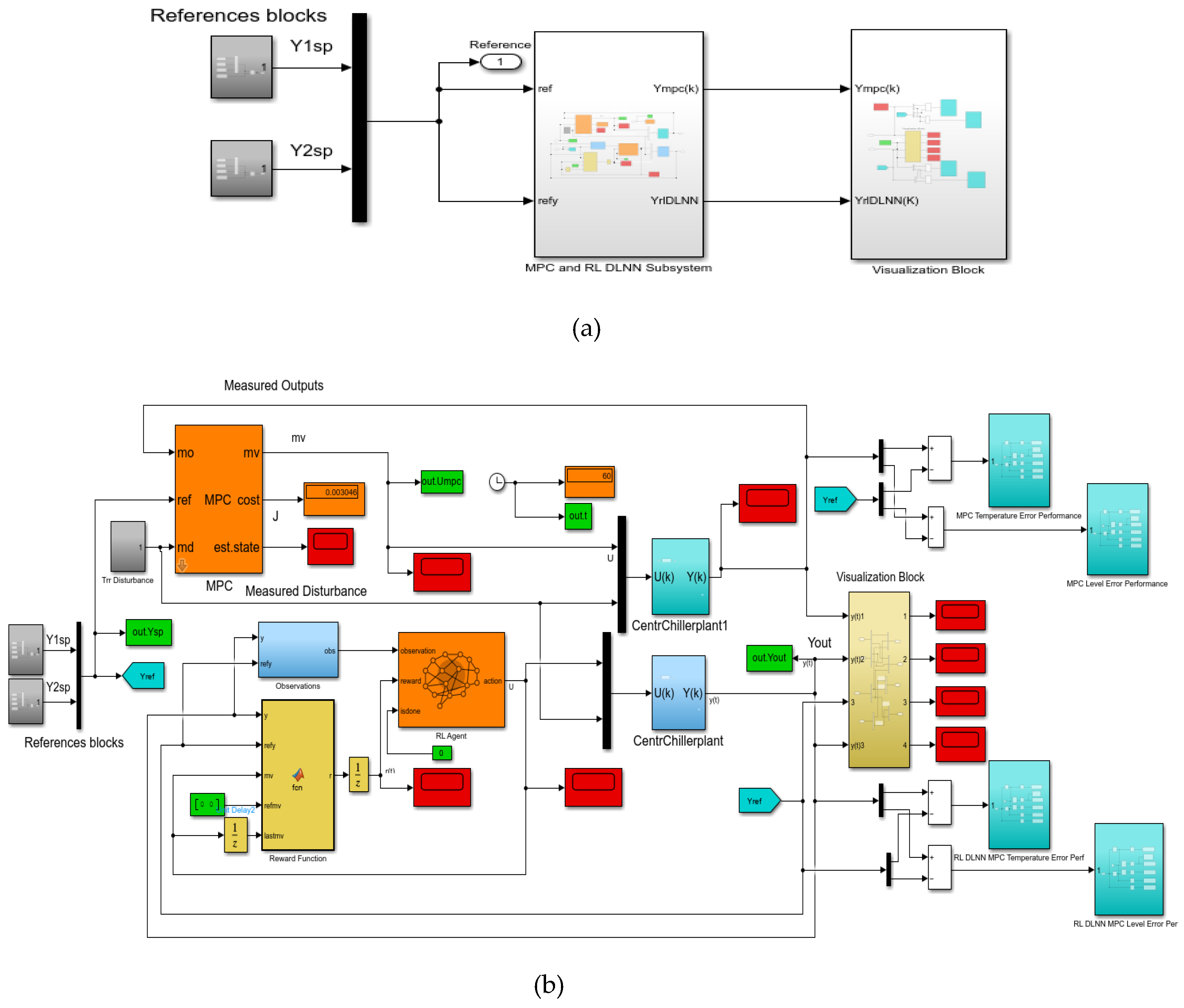
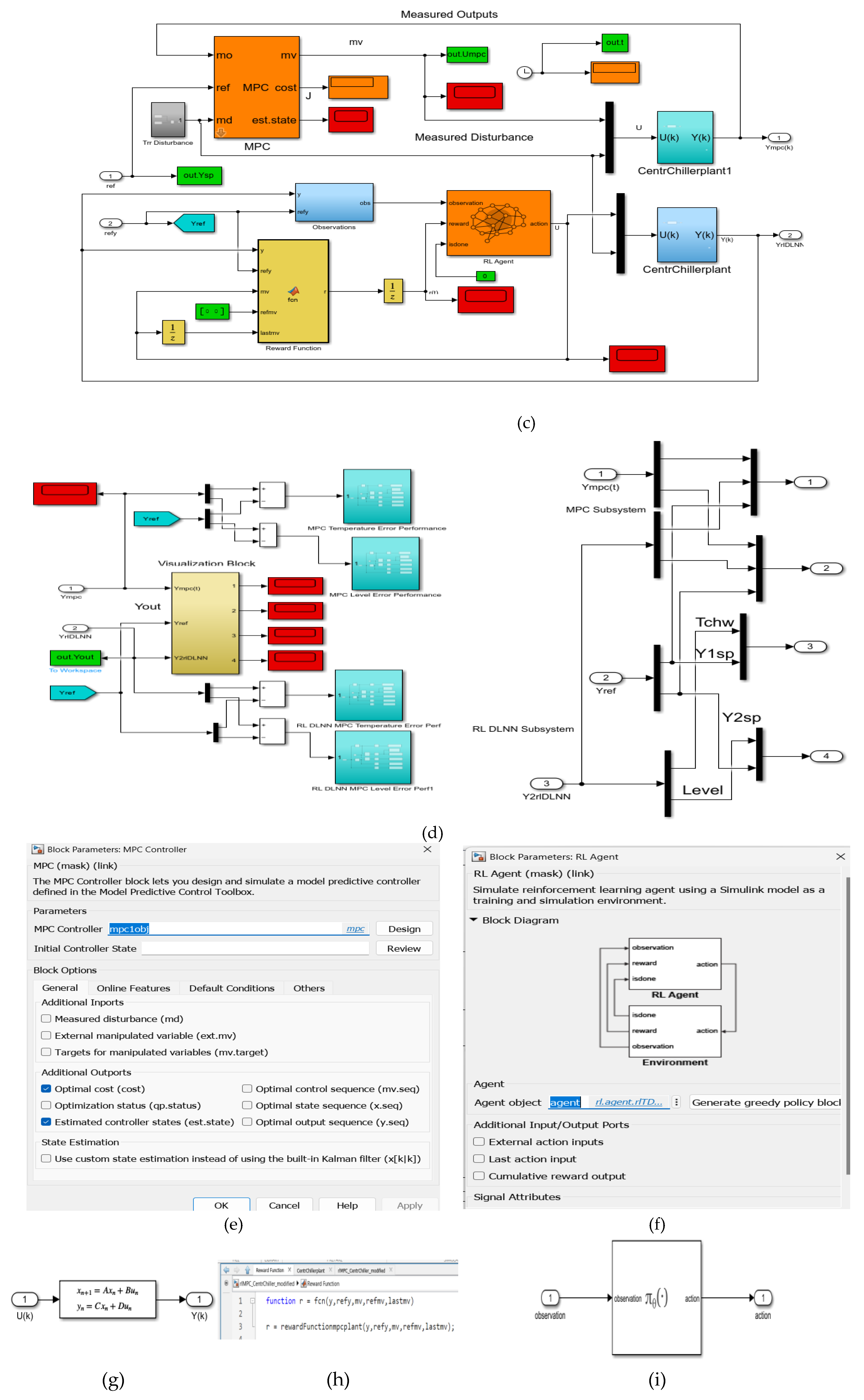
This intelligent control strategy implemented in MATLAB Simulink and presented in a compact and detailed architecture in Figure 9a-d is of practical interest that automatically generates the reward function from the cost and constraint. specifications defined in a Simulink model predictive controller (MPC) object. It is connected in a closed loop with the MIMO centrifugal cooling plant MIMO model given by Eq. (6) and Eq. (7) of section 2.2 to control the chilled water temperature Tchw-sp in the Evaporator subsystem and the liquid refrigerant level in the second condenser subsystem, depicted in the state space representation shown in Figure 9g. To implement this control strategy follows the same procedure that is well described in the MathWorks documentation updated to MIMO Centrifugal Chiller System (CCS) model [37,38]. The MPC object appearing at the top of Figure 9b and Figure 9c with its parameters block depicted in Figure 9e is created based on the direct CCS MIMO model using an inline MATLAB code procedure.
The RL DLNN Algorithm has the following steps:
- Step1:
- Create the MPC controller
- Step 1.1:
- Specify input and output signal types for the MPC controller. Two measured outputs are under consideration:
- The chilled water temperature Tchw inside the Evaporator is the first output
- The liquid Refrigerant Level within Condenser is the second output
- Step 1.2:
-
Specify constraints on the manipulated variable, and define a scale factor.mpc1obj.MV = struct('Min',{0 ; 0}, 'Max', {1.1; 1}, 'RateMin', {-1000;-1000},ScaleFactor= {1.1; 1});
- Step 1.3:
-
Specify the output constraints and the scale factors for both.mpc1obj.OV = struct('Min', {0;0},'Max',{10; 52},ScaleFactor ={10;52});
- Step 1.4:
-
Specify weights for the quadratic cost function to achieve temperature Tchw and Level tracking.mpc1obj.Weights = struct(MV=[0 0], MVRate=[0.1 0.1], OV=[0.1 0.1]);
- Step 1.5:
-
Create an MPC controller for the plant model with a sample time of Ts = 0.1 s, a prediction horizon m =10 steps, and a control horizon of p = 2 steps, using the previously defined structures for the weights, manipulated variables, and output variables. To capture all the dynamics evolution for both outputs the simulation time is set to Tf = 60 seconds.mpc1obj = mpc(plant, 0.1, 10, 2, mpc1obj.Weights,mpc1obj.MV,mpc1obj.OV);
- Step 1.6:
-
Display the controller specifications.mpc1obj
- Step2:
-
Generate the reward function code from specifications in the mpc object using the MATLAB code line:generateRewardFunction (mpc1obj)displayed in the MATLAB Editor:
Remark1:
The generated reward function is a starting point for reward design.
The implementer can modify the function with different penalty function choices and tune the weights.
- Step 2.1:
-
Specifications from MPC object
-
Standard linear bounds as specified in 'OutputVariables', and 'ManipulatedVariables' properties:ymin = [0 0]; ymax = [10 52]; mvmin = 0; mvmax = 1.1; mvratemin = -1000; mvratemax = Inf;
-
Scale factors as specified in “OutputVariables”, and “ManipulatedVariables” properties:Sy = [10 52]; Smv = [1.1 1];
-
Standard cost weights as specified in “Weights” property:Qy = [0.1 0.1];Qmv = [0 0];Qmvrate = [0.1 0.1];
-
- Step 2.2:
-
Compute costdy = (refy(:)-y(:)) ./ SyT; dmv = (refmv(:)-mv(:)) ./ SmvT; dmvrate = (mv(:)-lastmv(:)) ./ SmvT;Jy = dyT * diag(Qy.^2) * dy;Jmv = dmvT * diag(Qmv.^2)* dmv;Jmvrate = dmvrateT * diag(Qmvrate.^2) * dmvrate;Cost = Jy + Jmv + Jmvrate;
- Step 2.3:
-
Compute penalty for violation of linear bound constraints
-
Penalty function weight (specify nonnegative):Wy = [1 1]; Wmv = [10 10]; Wmvrate = [10 10];
-
Use the following functions to compute penalties on constraints.
- ○
- For exteriorPenalty, specify the penalty method as step or quadratic.
- ○
- Set Pmv value to 0 if the RL agent action specification has appropriate “LowerLimit” and “UpperLimit” values.
-
Penalty functions:Py = Wy* exteriorPenalty(y,ymin,ymax,'step');Pmv = Wmv * exteriorPenalty(mv,mvmin,mvmax,'step');Pmvrate = Wmvrate * exteriorPenalty(mv-lastmv,mvratemin,mvratemax,'step');Penalty = Py + Pmv + Pmvrate;
-
- Step 2.4:
-
Compute reward depicted as the output of MATLAB function block from Figure 12h.reward = -(Cost + Penalty);
Remark 2:
For tracking Tchw and Level setpoints, the implementer can make several changes and tune the parameters , such as:
- For exteriorPenality choose the penalty method quadratic instead step.
- Set the value of Penalty in the reward relationship to 6.
- Tune penalty function weights, Wy, Wmv, Wmvrate.
Remark 3:
The reward function is used to train reinforcement learning agent RL Agent, shown in Figure 9f.
- Step 3:
-
Create a reinforcement learning environmentThe environment dynamics are modeled in the CentrChillerPlant subsystem.The environment specifications are the following:
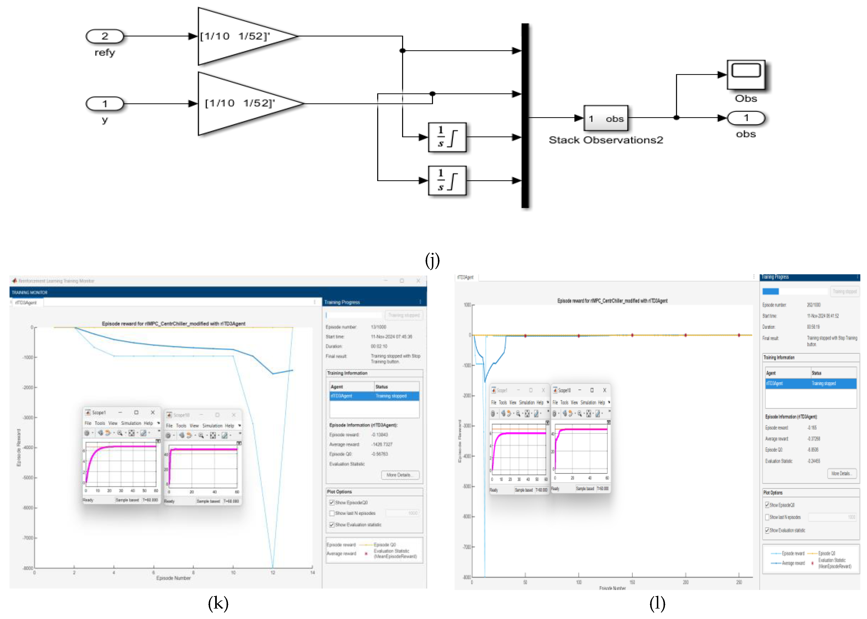
- The observations are the reference signals (Y1sp and Y2sp), output variables (Tchw and Level), and their integrals, as is shown in Figure 9j.
- The Tchw and Level signals are normalized by multiplying with the gain [1/10 1/52].
- The action is Ucom and u_EXV, limited between [0 1.1] for Ucom and [0 1] for u_EXV.
- The sample time and total simulation time are Ts = 0.1s and Tf = 60s, respectively.
- Step 3.1:
- Create the reinforcement learning environment using the rlSimulinkEnv function.
- Step 3.2:
- Create a Reinforcement Learning Agent with the Block parameters RL Agent shown in Figure 9f.
The agent used in this case study is a twin-delayed deep deterministic policy gradient (TD3) agent [38]. It uses two parametrized Q-value function approximators to estimate the value (that is the expected cumulative long-term reward) of the policy, as shown in Figure 9f and Figure 9i. To model the parametrized Q-value function within both critics, use a neural network with two inputs (the observation and action) and one output which correspond to the value of the policy when taking a given action from the state corresponding to a given observation, as is shown in Figure 9i.
- Step 3.3:
- Define each network path as an array of layer objects, and assign names to the input and output layers of each path in order to connect the paths.
- Step 3.4:
- Create layer graph object and add layers (criticNet), as is shown in Figure 10a.
- Step 3.5:
- Create the critic function objects using rlQValueFunction in order to encapsulate the critic by wrapping around the critic deep neural network. To make sure the critics have different initial weights, explicitly initialize each network before using them to create the critics, critic 1 and critic 2 [38]
TD3 agent learn a parametrized deterministic policy over continuous action spaces, which is learned by a continuous deterministic actor. This actor takes the current observation as input and returns as output an action that is a deterministic function of the observation. To model the parametrized policy within the actor, a neural network is used with one input layer (which receives the content of the environment observation channel) and one output layer (which returns the action to the environment action channel) [38].
- Step 3.6:
- Create actor network, namely actorNet, whose layer graph is shown in Figure 10b.
- Step 3.7:
- Create a deterministic actor function that is responsible for modeling the policy of the agent.
- Step 3.8:
- Specify the agent options and train the agent from an experience buffer of maximum capacity 1e6 by randomly selecting mini-batches of size 256. The discount factor of 0.995 favors long-term rewards as is stated in [38].
- Step 3.9:
- Specify optimizer options for the actor and critic functions, such a learn rate of 1e-3 and a gradient threshold of 1, as is set in [38].
Remark 4:
During training, the agent explores the action space using a Gaussian action noise model. Set the standard deviation and decay rate of the noise using the ExplorationModel property, as is done in [38].
- Step 3.10:
- Training RL Agent using train function, such is shown in Figure 9k after 13 epochs where is obtained the best tracking performance for chilled water temperature inside the Evaporator and for liquid Refrigerant Level within Condenser. Also, in Figure 12 l is shown the results of training process after 262 epochs, when the tracking performance of the liquid Refrigerant Level in Condenser is the best and for chilled water temperature inside the Evaporator is a little bit attenuated compared to the first result obtained in Figure 9k.
Figure 9.
Reinforcement learning control strategy based on Deep Neural Network of MIMO Centrifugal Chiller simplified model in state space reprezentation; (a) Simulink compact diagram of MIMO Centrifugal Chiller Plant and RL DLNN; (b)Detail Simulink diagram; (c) MPC and RLDNN Subsystem ; (d) Visualization block; (e ) MPC Prameters Block; (f) RL Agent block (controller); (g) State-Space reprezentation block; (h) Reward function; (i) RL Agent greedy policy block; (j) Observations block-detail; (k) Agent training process print screen snapshot after 13 epochs; (l) Agent training process print screen snapshot after 262 epochs.
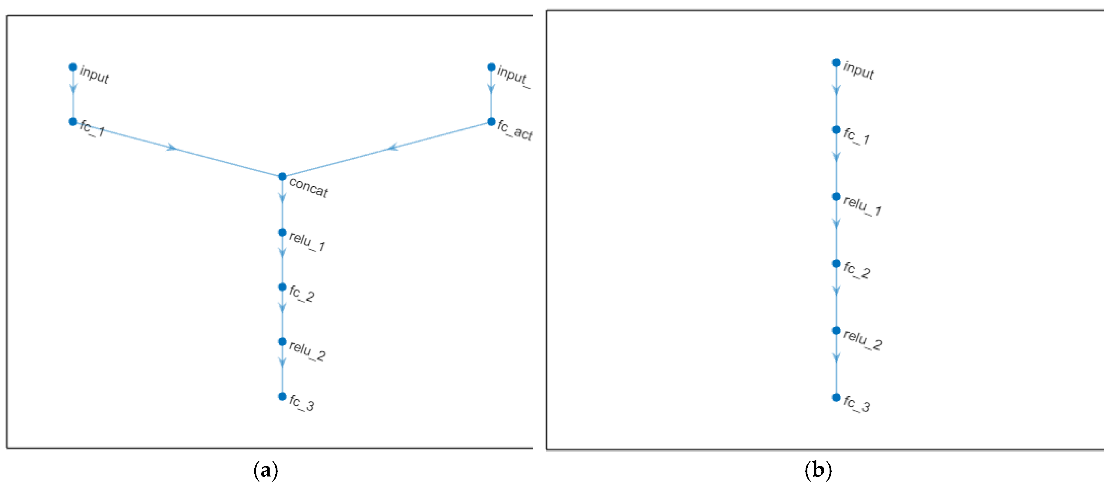
The layer graphs of criticNet and actorNet are displayed in Figure 13(a) and Figure 13(b), respectively.
Figure 10.
Layer graphs for criticNet and actorNet; (a) criticNet; (b)actorNet.
4.2.1. Reinforcement Learning Deep Learning Neural Network control strategy – Generate Reward Function from a Step Response Specifications of MIMO Centrifugal Chiller Simplified Model in State Space Reprezentation
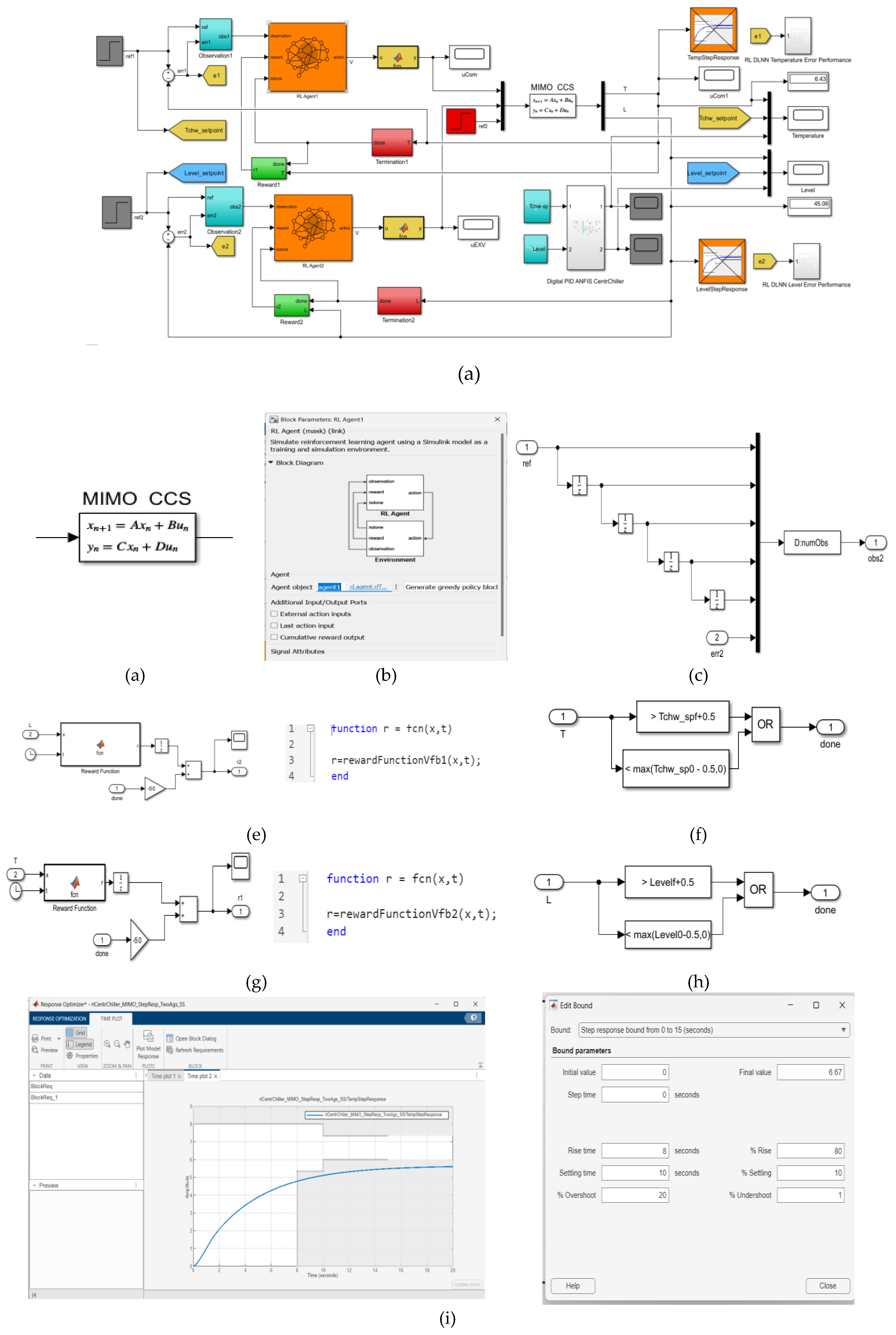
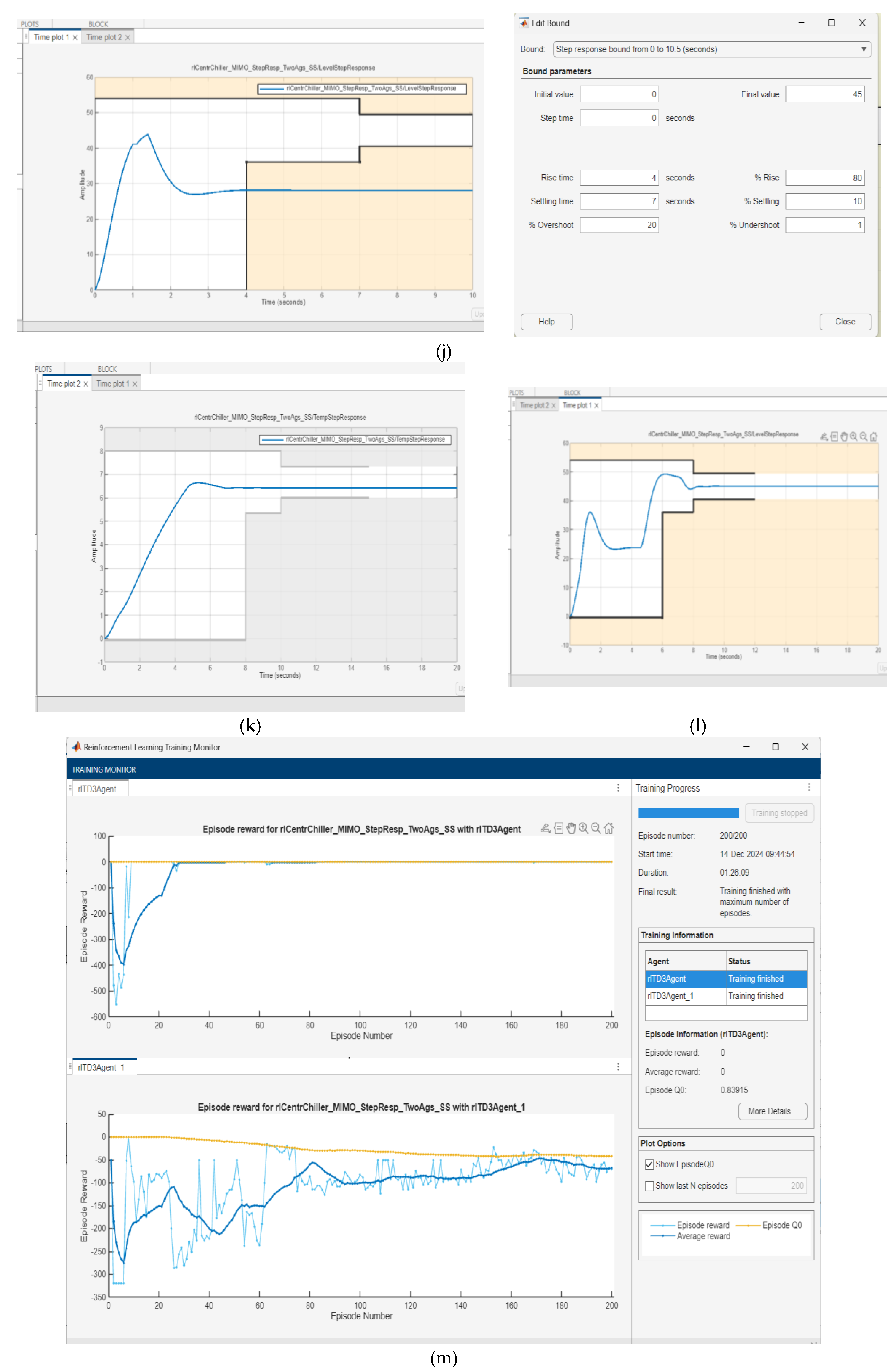
The both Digital PID and RL DLNN closed loop control strategies in a compact Simulink diagram architecture are depicted in Figure 14a. A description in state space of the MIMO CCS model that appears for performance comparison model in this diagram is made in Figure 11b. In Figure 11c is shown the Block Parameters of RL Agent1and in Figure 11d is detailed the Observations Block as component of same compact Simulink diagram. Also, the compact Simulink diagram shows how to automatically generate two reward functions rewardfunctionVfb1 and rewardfunctionVfb2 shown in Figure 11e and Figure 11g from performance requirements defined in a Simulink® Design Optimization™ model verification blocks for Evaporator Temperature control chosen as the first agent RL Agent1, and for Condenser liquid Refrigerant Level control as the second agent RL Agent2, respectively. Also, in the compact Simulink diagram appear two boolean logic termination blocks (Done), to stop the training of the RL Agent1 and RL Agent2 when the Evaporator Temperature and the Condenser Level reach a good accuracy performance, given in Figure 11f and Figure 11h. The rewardfunctionVfb1 and rewardfunctionVfb2 are used to train both reinforcement learning RL Agent1 and RL Agent2, following the steps and the MATLAB Reinforcement Learning soubrutine procedure similar to those developed in [37,40] applied for MIMO plants. The training of both agents RL Agent1 and RL Agent2 are performed similar to MPC RL DLNN described in previous Subsection 4.3.1. Compared to MPC RL DLNN the both RL agents are descentralized with two distinct paths. The untrained simulation results for Evaporator Temperature control and Condenser liquid Refrigerant Level control are exposed in Figure 11i and Figure 14j respectively. In Figure 11k and Figure 11l are presented the training simulation results for Evaporator Temperature and liquid Refrigerant Level inside of Condenser after 200/200 epochs, as is shown in Figure 11m.
The training process of both RL Agent1 and RL Agent2 is finished after the agents reached stop training criteria set in training options MATLAB subroutine:
trainOpts = rlMultiAgentTrainingOptions(…
AgentGroups = {1,2},…
LearningStrategy = (“descentralized”),…
MaxEpisodes = 200,…
MaxStepsPerEpisode = ceil(Tf/Ts),…
StopTrainingCriteria = “Average Reward”,…
StopTrainingValue = [1.1],…
ScoreAveragingWindowLength = 20);
The penalty function weight is specified nonnegative and set to:
Weight = 2
To compute the penalty for violation of linear bound constraints, it must use the following functions to compute penalties on constraints, namely the exteriorPenalty, barrierPenalty, hyperbolicPenalty. For exteriorPenalty the user specifies the penalty method as step or quadratic, for preference quadratic. The corresponding MATLAB code line inside the MATLAB block built based on the step response specifications of each rewardfunction is the following
Penalty = sum(exteriorPenalty(Block1_x, Block1_xmin, Block1_xmax, 'quadratic'))
The MATLAB Simulink simulations results are shown in next Section 6.2.
Figure 11.
Reinforcement Learning Deep Learning Neural Network Simulink diagram. (a) Overal Simulink diagram of RL DLNN control architecture and MIMO CCS (b)MIMO CCS state space model; (c) RL Agent1 block; (d)Observations block; (e) RewardFunctionVfb1 block; (f) The Termination Block for first RL Agent1; (g) RewardFunctionVfb block2; (h) The Termination Block for first RL Agent2; (i) The chilled water Temperature within Evaporator and Step response block specifications – untrained RL1 Agent; (j) The liquid Refrigerant Level inside Condenser and Step response block specifications – untrained RL Agent2; (k) The chilled water Temperature within Evaporator–trained RL1 Agent after 33/200 epochs; (l) The liquid Refrigerant Level inside Condenser – trained RL2 Agent after 33/200 epochs; (m) Training process of the agents RL1 and RL2.
5. Traditional and Advanced Intelligent Closed Loop Control Strategies – MATLAB Simulink Simulations Results
In this section are revealed the MATLAB Simulink simulations results of traditional closed loop control strategies in Subsection 5.1, namely DTI control of MIMO CCS in Subsection 5.1.1, PID control of MIMO CCS extended nonlinear model with 39 states, inputs subjected to constraints, and a measured temperature disturbance, an improved version of PID control, more precisely a Digital PID control of MIMO CCS ANFIS model in Subsection 5.1.3, Model Predictive Controller of MIMO CCS model represented in state space with four states in Subsection 5.1.4. Also, a reinforcement learning MPC Deep Learning Neural Networks (RL DLNNs) control of MIMO CCS model versus MPC control in Subsection 5.2.1, and RL DLNN control of MIMO CCS model in state space representation versus the improved version Digital PID control of MIMO CCS ANFIS model in Subsection 5.2.2.
5.1. Traditional Closed Loop Control Strategies
5.1.1. DTI Closed Loop Control
The simulation results are presented in Figure A2 from Appendix A. In Figure A2a is shown the Simulink diagram of DTI controller. In Figure A2b is depicted the DTI control of chilled water temperature control within Evaporator subsystem and in Figure A2c the liquid Refrigerant Level control inside Condenser subsystem respectively. In Figure A2d are shown the Compressor and Expansion Valve opening actuators control efforts.
5.1.2. PID Closed Loop Control – Centrifugal Chiller Extended Model (39 States)
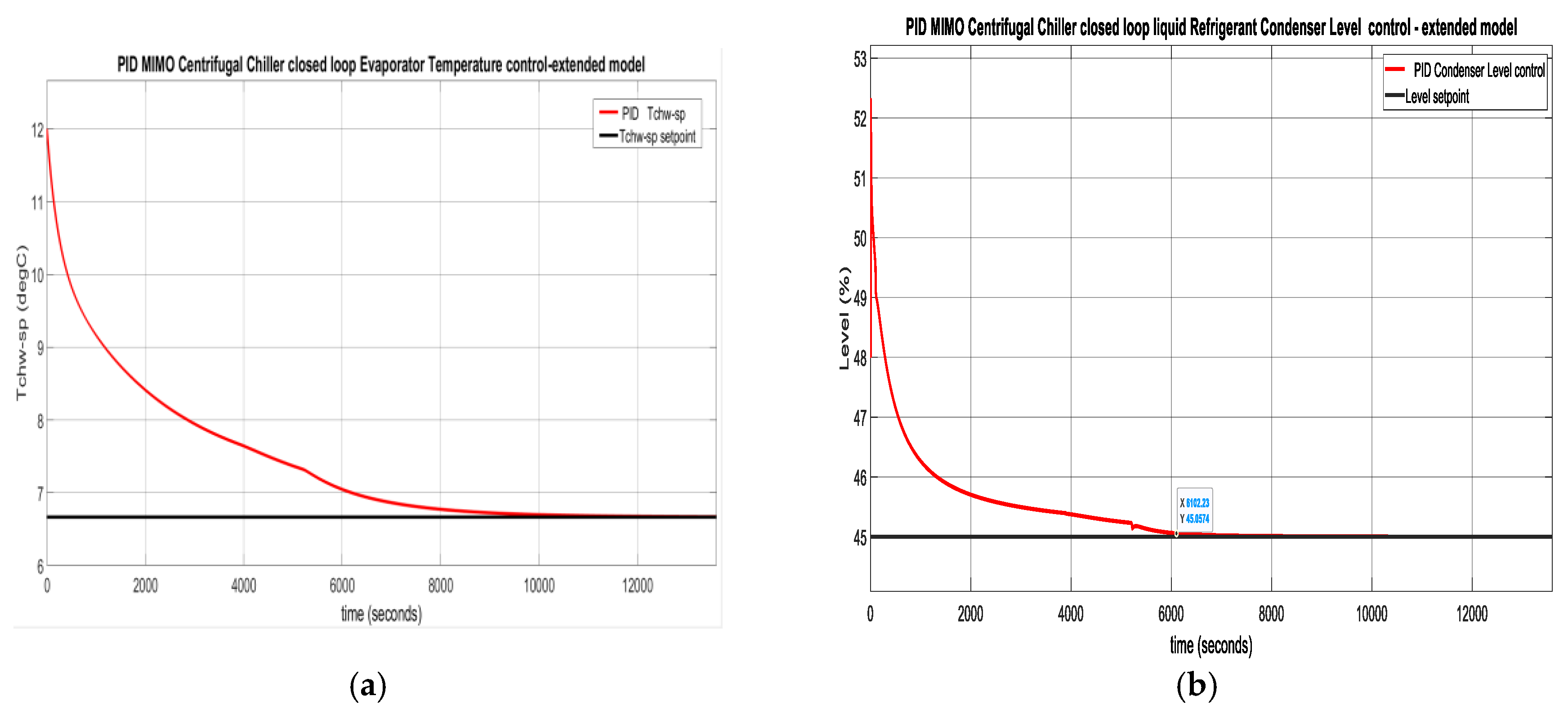
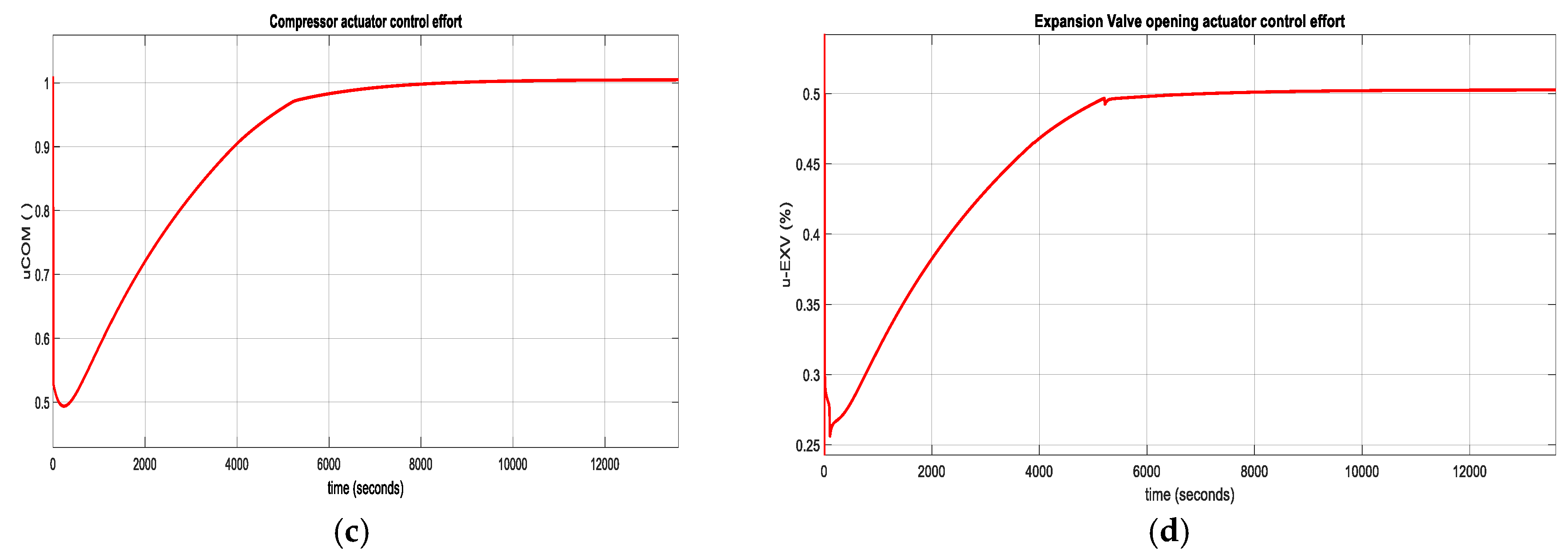
The Simulink simulations result is depicted in Figure 12. In Figure 12a is shown the PID MIMO Centrifugal Chiller closed loop Temperature control inside Evaporator Subsystem, while in Figure 12b is revealed the PID control of liquid Refrigerant Level within the Condenser Subsystem. Figure 12c depicts the Compressor actuator control effort and Figure 12d discloses the Expansion Valve opening actuator control effort.
Figure 12.
MATLAB Simulink simulations results. (a) PID Evaporator subsystem Temperature control ;(b) PID Liquid refrigerant level control in Condenser subsystem; (c) The Compressor relative speed actuator control effort ; (d) The expansion valve opening actuator control effort.
Figure 12.
MATLAB Simulink simulations results. (a) PID Evaporator subsystem Temperature control ;(b) PID Liquid refrigerant level control in Condenser subsystem; (c) The Compressor relative speed actuator control effort ; (d) The expansion valve opening actuator control effort.
5.1.3. Digital PID Control of MIMO Centrifugal Chiller ANFIS Model
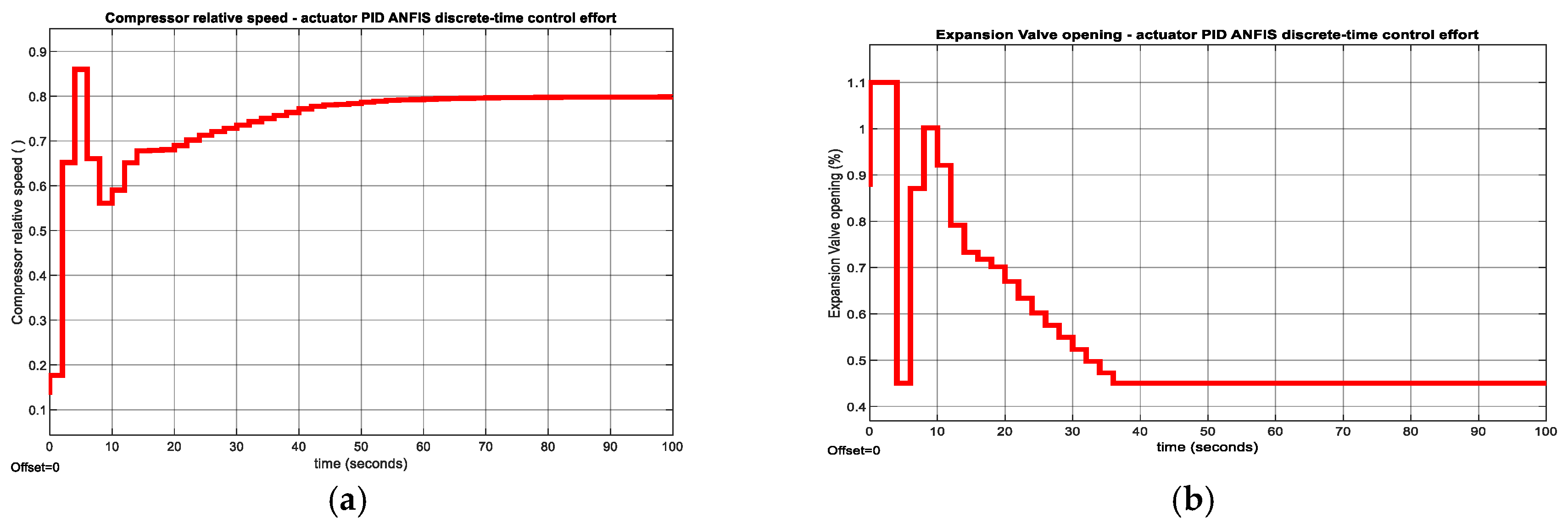
The MATLAB Simulink simulations result is revealed in the Figure 14, Figure 15, and Figure A4, Figure A5, Figure A6 and Figure A7 from Appendix A. The MATLAB Simulink simulation of results digital PID control CCS ANFIS model without changes in temperature and level setpoints are depicted in the Figure 14a and Figure 14b respectively. The actuators control efforts for Compressor and Expansion Valve opening are shown in Figure 15a and Figure 15b correspondingly. At a simple visual inspection of both figures it seems that the fast Digital PID control has a fast step response, reaching a zero steady-state for a settlig time of 50 seconds with a 9% overhoot for chilled water inside Evaporator and 2% for liquid Refrigerant level within Condenser.
Figure 14.
MATLAB Simulink simulation results without changes in temperature and level setpoints. (a) PID ANFIS discrete-time control of Tchw-sp in Evaporator; (b) PID ANFIS discrete-time control of liquid refrigerant level in Condenser.
Figure 14.
MATLAB Simulink simulation results without changes in temperature and level setpoints. (a) PID ANFIS discrete-time control of Tchw-sp in Evaporator; (b) PID ANFIS discrete-time control of liquid refrigerant level in Condenser.
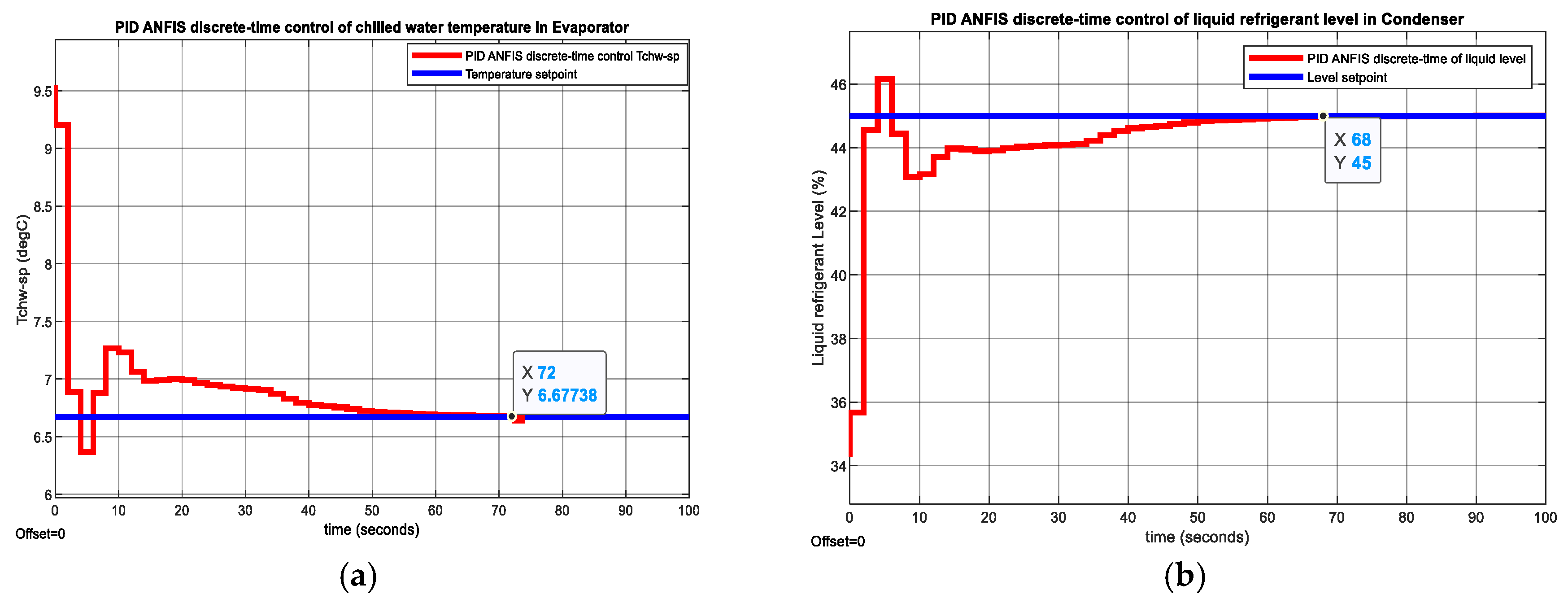
Figure 15.
PID ANFIS discrete-time control - MATLAB Simulink simulation results of actuators control efforts. (a) Compressor relative speed; (b)Expansion valve opening.
Figure 15.
PID ANFIS discrete-time control - MATLAB Simulink simulation results of actuators control efforts. (a) Compressor relative speed; (b)Expansion valve opening.
The ability of the Digital PID controller to reject the effect of temperature disturbance is revealed in Figure A4a for temperature and in Figure A4b for liquid Refrigerant level, respectively. In Figure A5a is shown the impact of same temperature disturbance on the Compressor actuator control effort, and in Figure A5b on Expansion valve opening actuator effort, respectively. Moreover, in Figure A6a is shown the evolution of the chilled water temperature inside the Evaporator subsystem, and in Figure A6b is disclosed the liquid refrigerant level evolution within the Condenser subsystem to changes in setpoint values for temperature and level, respectively. The impact of these setpoints changes on Compressor and Expansion Valve opening actuators control efforts are shown in Figure A7a and Figure A7b correspondingly.
5.1.4. Model Predictive Control of MIMO Centrifugal Chiller Nonlinear Extended Model in State Space Representation (39 States) with Input Constraints
The MPC simulations result are decripted in Figure 16a-e. The both actuators, Compressor relative speed and Expansion Valve opening control efforts are represented in Figure 16a. The Figure 16b reveals the chilled water temperature disturbance, Trr. In Figure 16c is shown the MPC of chilled water temperature (OV1) inside the Evaporator in degrees Celsius, and in Figure 16d is displayed the liquid Refrigerant level (OV2) within Condenser for a change in Temperature disturbance Trr from 48 [degF] to 54 [degF] applied at time instant t = 40 [s]. Figure 16e displays the four estimated states of MIMO centrifugal chiller based on Kalman Filter state estimation algorithm.
5.2. Advanced Reinforcement Learning Using Deep Learning Neural Networks Control Strategies
In this section is presented the simulation results of advanced reinforcement learning deep learning neural networks (RL DLNN) developed in previous Section 4 conducted on MATLAB Simulink R2024 software programming platform.
In the next Subsection 5.2.1 is shown the Simulink simulations result for RL DLNN that generates the reward function from a MPC dataset extracted from MIMO CCS simplified model represented in state space given in Eq. (7) and in Subsection 5.2.2 is exposed the simulations result for RL DLNN that generates the reward function from two step responses’ block specifications of same MIMO CCS simplified model in state space representation.
5.2.1. Reinforcement Learning Deep Learning Neural Network Control Strategies–Generate Reward Function from MPC of MIMO Centrifugal Chiller Simplified Model in State Space Reprezentation
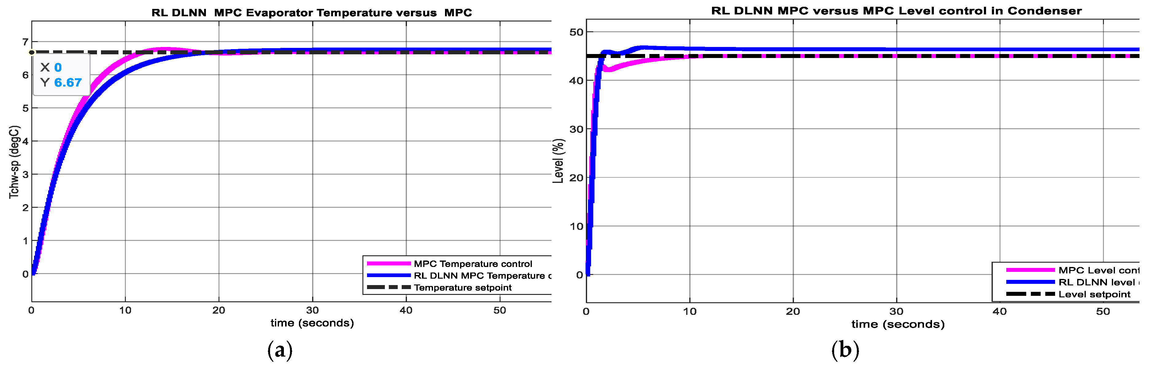
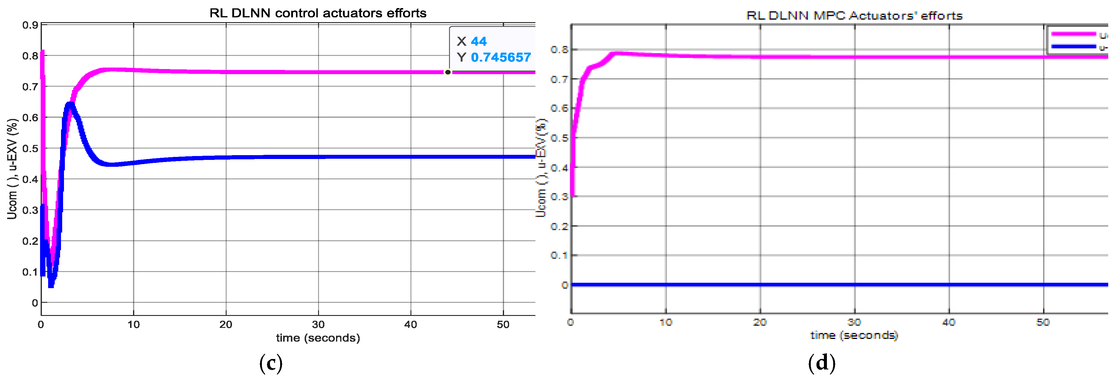
The Simulink simulations result is shown in Figure 17a-d. The RL DLNN control of Evaporator chilled water Temperature result is displayed in Figure 17a, and in Figure 17b is represented the liquid Refrigerant Level within Condenser, both versus their corresponding MPC step responses on the same graphs. The MPC control efforts are revealed in Figure 17c and in Figure 17d are illustrated the RL DLL MPC control efforts, separately.
Figure 4.
RL DLNN – Generate Reward Function based on MPC specifications. (a) RL DLNN MPC Evaporator Temperature control versus MPC ; (b) RL DLNN MPC Condenser Level control versus MPC; (c) MPC control actutators efforts; (d) RL DLNN MPC Actuators efforts.
Figure 4.
RL DLNN – Generate Reward Function based on MPC specifications. (a) RL DLNN MPC Evaporator Temperature control versus MPC ; (b) RL DLNN MPC Condenser Level control versus MPC; (c) MPC control actutators efforts; (d) RL DLNN MPC Actuators efforts.
5.2.2. Reinforcement Learning Deep Learning Neural Network control Strategies – Generate Reward Function from a Step Response Specifications of MIMO Centrifugal Chiller Simplified Model in State Space Reprezentation
The simulations result of RL DLNN control of Evaporator chilled water Temperature is depicted in Figure 18a and in Figure 18b for liquid Refrigerant level versus Digital PID control of MIMO ANFIS model responses.
The RL DLNN actuators control efforts are illustrated in Figure 18c for Compressor and in Figure 18d for Expansion Valve opening respectively, while the control efforts of Digital PID control of CCS ANFIS models are ahown in Figure 18e for Compressor actuator and Figure 18f for Expansion Valve opening actuator.
6. Discussions
6.1. Traditional Closed Loop Control Strategies
In this section a rigurous performance analysis is made based on the data statistics and stability performance error indicators extracted from step responses and the standard structures that claculate these indicators, such as ISE, ITSE, IE, IAE, and ITAE.
6.1.1. DTI Controllers
For the discrete-time integrator (DTI) controller developed in Section 3.1, by a simple inspection of both step responses represented in Figure A2ab and the data statistics extracted from the same step responses for Evaporator temperature depicted in Figure 19a, and liquid refrigerant level inside Condenser displayed in Figure 19b disclose the following performances during transient and steady state regimes, namely acceptable time responses (settling time, Ts) and rise time (Tr) for temperature Ts=40, Tr = 5.5 seconds and for liquid Refrigerant level Ts=20, Tr=1.7 seconds, an overshoot of σ_max= 45.27% for temperature and a larger number of maximum amplitude oscillations of about 10%, and both reaching zero steady state errors, therefore a high tracking accuracy.
A mean = 7.071 and standard deviation std =1.708 for DTI temperature control is extracted from Figure 19a, as well as a mean = 44.43 and std =7.759 for DTI liquid Refrigerant level control is given in Figure 19b. It is also worth noting the strong control effort of the oscillating Compressor and the almost smooth opening of the Expansion valve.
6.1.2. PID Control MIMO Centrifugal Chiller System Extended Model – 39 States
The step responses shown in Figure 12a and Figure 12b reveal a very long Ts =10000 seconds,Tr=10000 seconds, no overhoot, zero steady-state error, smooth Compressor control effort for PID Temperature control and a very long Ts = 6000, Tr = 6000seconds, no overhoot, zero steady-state error, smooth Expansion Valve opening control effort for PID Level control. The main issues encountered for this closed loop control strategy are a very slow time response and an accurate tuning procedure of parameter values. Also, a mean = 7.405 and standard deviation std = 0.9972 for PID temperature control are revealed in Figure 20a and the mean = 45.03 and std =0.7477 for PID Level control are shown in Figure 20b.
6.1.3. Model Predictive Control of MIMO Centrifugal Chiller Simplified Model in State Space Representation
A rigurous performance analysis of step responses depicted in Figure 16c for Evaporator temperature subsystem and in Figure 16d for liquid Refrigerant level of Condenser subsystem reveals the following features:
- a settling time Ts = 24.6 seconds and a rising time Tr = 7.6 seconds, an overshoot of σ_max = 6.75%, zero steady-state, and an excellent disturbance rejection for Evaporator temperature control
- a settling time Ts=7.2 seconds,and rising time Tr=7.2 seconds,no overshoot, a high tracking performance accuracy, and great disturbance rejection recommands for liquid Refrigerant level inside Condenser subsystem
which recommand the MPC closed-loop strategy among the most suitable conventional control strategies that performs very well. Furthermore, both inputs Compressor relative speed and Expansion Valve opening doesn’t violate the linear bound constraints. Lets why the MPC is adopted in the first RL DLNN closed loop control strategy developed in Section 4.3.1 to generate the reward function from MPC specifications of MIMO centrifugal chiller system model proposed in the case study.
6.2. Advanced Intelligent Closed Loop Neural Control Strategies
6.2.1. Digital PID Control MIMO CCS MISO ANFIS Models
The MATLAB Simulink simulation results of digital PID control CCS ANFIS model without changes in temperature and level setpoints depicted in the Figure 14a and Figure 14b respectively are showing a fast time response Ts = 50 seconds of Evaporator temperature control subsystem, a zero steady-state error with a 9% temperature of chilled water overhoot compared to liquid Refrigerant level control inside Condenser subsystem with Ts = 64 seconds, steady state error, and 2% overshoot of the liquid Refrigerant level in Condenser. Moreover, the actuators control efforts for Compressor and Expansion Valve opening shown in Figure 15a and Figure 15b correspondingly are sharp at the beginning and smooth after. The Simulink simulation results depicted in Figure A4a and Figure A4b reveal that the effect of changes in disturbance Temperature load Trr from 48 to 54 degrees Fahrenheit applied at time t=70 seconds is completely rejected for the chilled temperature control inside the Evaporator, as well as for the liquid refrigerant Level within Condenser, almost in 40 seconds. Also, it is obvious that the steady state for both controlled outputs is very close to zero, and the settling times of the step responses are faster enough for both Digital PID controllers, which can be interpreted as an excellent performance of the improved Digital PID control strategy, outperforming the previous control PID control strategy based on extended model developed in Section 3.2. Lets why the Digital PID with the proposed tuning procedure of the parameters values is used for comparison performance in the second RL DLNN control structure.
6.3. Advanced Reinforcement Learning Deep Learning Neural Networks Control Strategies
For a rigurous tracking performance analysis is essential purpose to minimize the error in any feedback closed loop control system and hence in order to keep track of the errors at all time from zero to infinity, and to minimize them continuously a performance measure in terms of Integral time absolute error (ITAE), Integral square error (ISE), Integral time square error(ITSE) and Integral absolute error (IAE) such those defined in [35] and given by the Eqs. (18)-(22).
Also, an effective tracking performance measure uses data statistics such as min, max, mean, median, mode, standard deviation (std), and range, as shown in Figure A8a-d, Figure A10a-d. In Ref. [35] the Integral time indicators defined by Eqs.(18)-(21) are so-called fitness functions with the values calculated by the standard hardware structures shown in Figure A9a-d and Figure A11a-d, and define as:
Specifically, all of these time integral criteria are generic and comprehensive tools to evaluate the performance of a control system. Hence, a system may have a good rise time but a poor settling time, or vice versa, other basic criteria for evaluating the step response tracking performance of a closed loop feedback system are the overshoot, the steady state error extracted from the data statistics tables, but all these statistics describe only one characteristic, the time integral criteria are generic and comprehensive, they allow comparison between different controller designs or even a different structure of the controller. The fitness functions are not actually limited to the above equations. Engineers can provide custom fitness functions depending on the target design and control system. The overall performance (convergence speed and optimization accuracy) of an interesting evolutionary algorithm developed in [35] for tuning the PID parameters values at optimal values depends on the fitness functions. Note that integral time absolute error (ITAE) is widely used in control processing since it is simple to implement and natural to define energy of a signal, which possesses symmetry and differentiability.
6.3.1. Reinforcement Learning Deep Learning Neural Network Control Strategies –Generate Reward Function from a MPC of MIMO Centrifugal Chiller Simplified Model in State Space Reprezentation
The Data Statistics Tables for RL DLNN Temperature and Level control algorithms versus mpc of Evaporator Temperature and Condenser Refrigerant Level are shown in the Figure A8a-d. The Figure A8a presents the statistics data for mpc Evaporator Temperature control, Figure A8b is for RL DLNN mpc Temperature control, Figure A8c is viewing data statistics for mpc Condenser Refrigerant Level, and Figure A8d is seeing for RL DLNN mpc Refrigerant Level control. The performance error indicators values are extracted from the hardware structures from Figure A9a-d, more precisely for mpc Evaporator temperature in Figure A9a, RL DLNN mpc Evaporator temperature in Figure A9b, mpc Condenser Refrigerant level in Figure A9c, and finally RL DLNN mpc Condenser Refrigerant in Figure A9d. An attentive performance analysis based on the data statistics for the MPC RL DLNN Evaporator temperature control Subsystem reveals a slight superiority compared to MPC based on the corresponding data statistics and vice versa for the Condenser liquid level control Subsystem. Regarding the final values of fitness functions values after 60 iterations, the Simulink simulations results indicate a slight superiority of MPC RL DLNN Evaporator Temperature control Subsystem compared to MPC and vice versa for the Condenser liquid level control Subsystem. The MPC RL DLNN performs better for temperature control and is slightly close to liquid refrigerant level control. After many other repetitions of the tuning parameter values procedure, thus a so-called “trial and error” procedure, the performance of MPC RL DLNN simulation results could change significantly such that it can finally outperform the conventional MPC for both, temperature and liquid Refrigerant level control. Our investigations will continue to improve the MPC RL DLNN controller performance in future work.
6.3.2. Reinforcement Learning Deep Learning Neural Network Control Strategies – Generate Reward Function from a Step Response Specifications of MIMO Centrifugal Chiller Simplified Model in State Space Reprezentation
Similarly, the Data Statistics Tables for RL DLNN Temperature and Level control algorithms versus Digital PID control-CCS ANFIS model of Evaporator Temperature and Condenser Refrigerant Level are shown in the Figure A10a-d. The Figure A10a presents the statistics data for RL DLNN Evaporator Temperature control, Figure A10b is for Digital PID Temperature control CCS ANFIS model, Figure A10c is viewing data statistics for RL DLNN Condenser Refrigerant Level, and Figure A10d is seeing for Digital PID Refrigerant Level control CCS ANFIS model. The performance indicators values are extracted from the hardware structures from Figure A11a-d, more precisely for RL DLNN Evaporator Temperature in Figure A11a, Digital PID Evaporator Temperature control-CSS ANFIS nodel in Figure A11b, RL DLNN Condenser Refrigerant Level in Figure A11c, and finally Digital PID Condenser Refrigerant Level control CCS ANFIS model in Figure A11d. Similar to MPC RL DLNN a rigorous performance analysis made for RL DLNN based on the data statistics and fitness functions' final values after 60 iterations indicates a slight superiority of the improved Digital PID controller connected in the same forward-path closed loop architecture with the MISO ANFIS CCS models compared to the RL DLNN performance, but the both controllers outperforms the standard PID controller. Furthermore, by increasing the number of “trial and error” procedures of tuning parameter values, for sure the performance of RL DLNN results can change significantly and finally it can outperform the improved Digital PID control structure for both, temperature and liquid Refrigerant level control. Our investigations will continue in this direction in future work.
7. Conclusions
Some of the issues/challenges were revealed in this research paper, focusing on the nonlinearity and high dimensionality of MIMO CCS (39 states), strongly constrained inputs, modelling errors, temperature perturbations, reference tracking issues, and low-level graphics to solve. The valuable results obtained demonstrate that our investigations to build both advanced neural intelligent RL DLNN controllers were successful. The MATLAB Simulink simulation results reveal that the first advanced MPC RL DLNN controller performs very close to an MPC, and the second one outperforms the standard PID, but performs very close to the improved Digital PID CCS ANFIS model structure. Finally, you can see that the first MPC RL DLNN controller has a slight superiority compared to the Digital PID RL DLNN controller. The preliminary results of our investigations carried out in this research paper were successful, and of real interest, fulfilling the main objective of this research. Even though the results of MATLAB Simulink simulations are exciting but not excellent, the great gain of this research work is a significant progress and a rich experience accumulated in building such RL DLNN control algorithms. For future work, research continues in the direction of improving both RL DLNNs investigated in this paper by designing and implementing new advanced intelligent learning and neural control techniques as a viable alternative to the traditional ones.
Author Contributions
Conceptualization, N. Tudoroiu; methodology, D. Curiac and N. Tudoroiu; software, D. Curiac and R-E. Tudoroiu; validation, M. Zaheeruddin and N. Tudoroiu.; formal analysis, R-E. Tudoroiu; investigation, N. Tudoroiu and D. Curiac; resources, S-M. Radu.; data curation, M. Zaheeruddin; writing—original draft preparation, R-E. Tudoroiu; writing—review and editing, N. Tudoroiu.; visualization, R-E. Tudoroiu and S-M Radu; supervision, N. Tudoroiu and M. Zaheeruddin; project administration, S-M. Radu.; funding acquisition, S-M. Radu. All authors have read and agreed to the published version of the manuscript.
Funding
This research received no external funding.
Acknowledgments
I want to express my gratitude to Roberta Silerova, John Abbott College Program Dean Science, Chair Mark Evanchyna and Co-Chair Hana Chammas of the Intech Department, as well as my department colleagues, Dr. Demartonne Ramos França, Dr. Shiwei Huang and M.Sc. Evgeni Kiriy, for their support, guidance and valuable advice during the course of this scientific research project. .
Conflicts of Interest
The authors declare no conflict of interest.
Abbreviations
The following abbreviations are used in this manuscript:
| PID | Proportional Integral Derivative |
| DTI | Discrete Time Integrator |
| HVAC | Heating Ventilation Air Condition |
| CCS | Centrifugal Chiller System |
| MIMO | Multi input Multi output |
| SISO | Single input Single output |
| MISO | Multi input Single output |
| ARMAX | Autoregressive Moving Average with Exogenous input |
| ANFIS | Adaptive Neural Fuzzy Inference System |
| IAE | Integral Absolute Error |
| ITAE | Integral Time Absolute Error |
| ISE | Integral Square Error |
| ITSE | Integral Time-weighted Square Error |
Appendix A
Appendix A.1. Figures
Figure A1.
The Simulink diagram of discrete-time transfer function of MIMO centrifugal chiller plant.
Figure A1.
The Simulink diagram of discrete-time transfer function of MIMO centrifugal chiller plant.
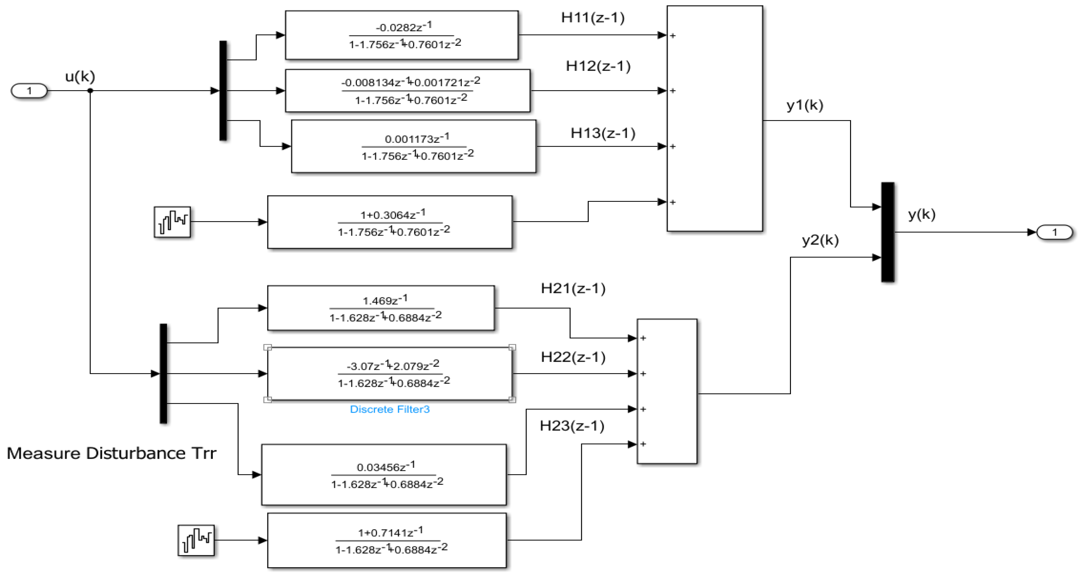
Figure A2.
DTI control - MIMO centrifugal chiller system extended model and Simulink simulations. (a) DTI control Simulink diagram; (a) Chilled water temperature in Evaporator;(b)Liquid refrigerant level in Condenser; (c) Compressor and Expansion Valve opening acctuators control efforts;.
Figure A2.
DTI control - MIMO centrifugal chiller system extended model and Simulink simulations. (a) DTI control Simulink diagram; (a) Chilled water temperature in Evaporator;(b)Liquid refrigerant level in Condenser; (c) Compressor and Expansion Valve opening acctuators control efforts;.
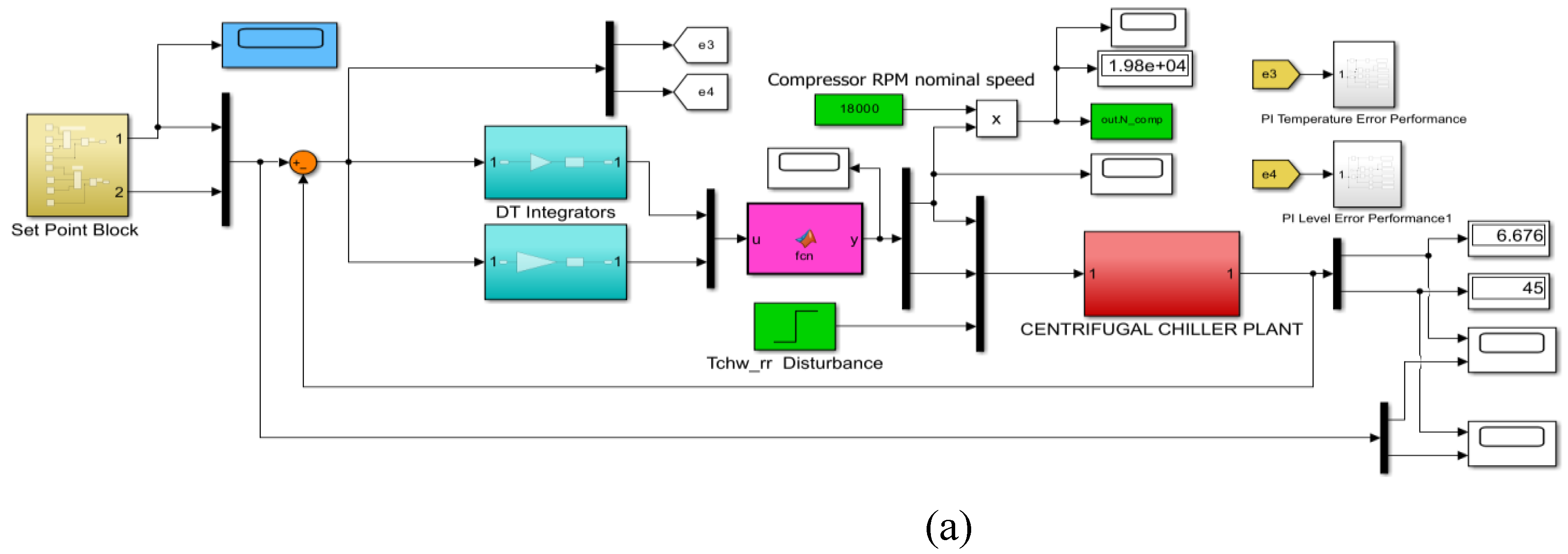
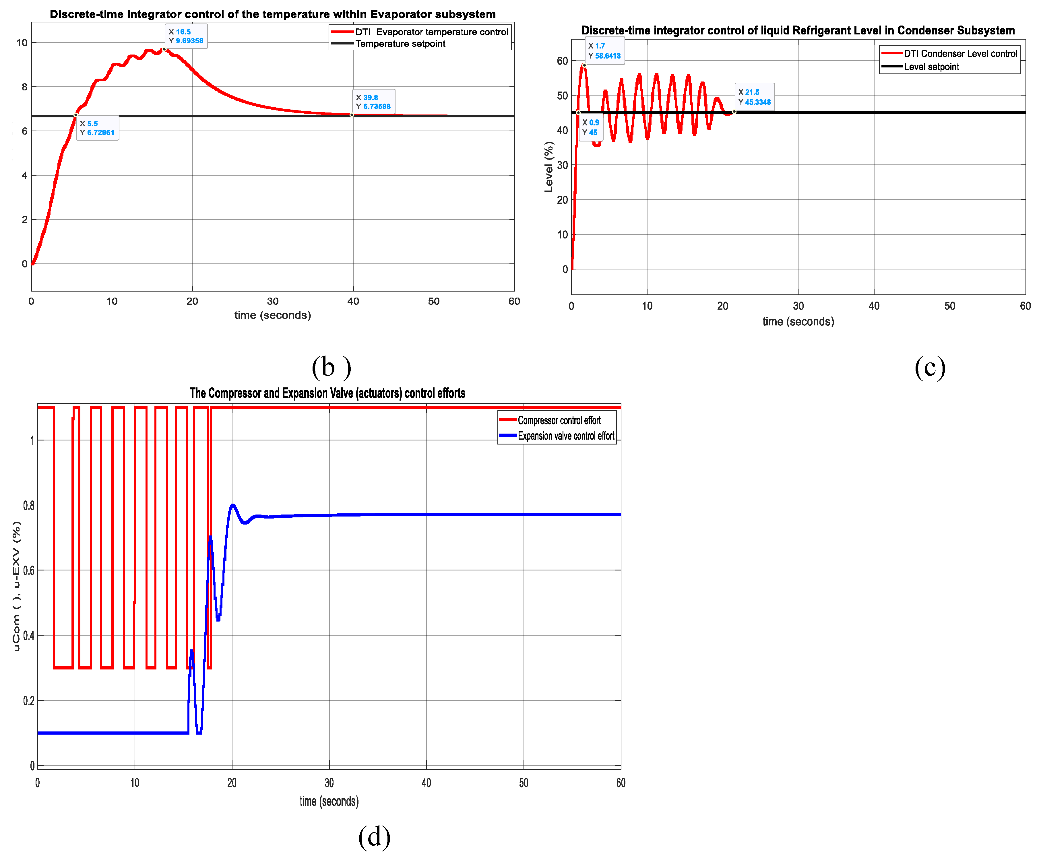
Figure A3.
The Simulink model for PID closed loop control strategies of Centrifugal Chiller MIMO nonlinear extended model (39 states). (a) Overall diagram; (b) Components of the Simulink block diagram (MATLAB Function of the extended model and MATLAB function visualization block) ; (c) MATLAB Function – Visualization block.
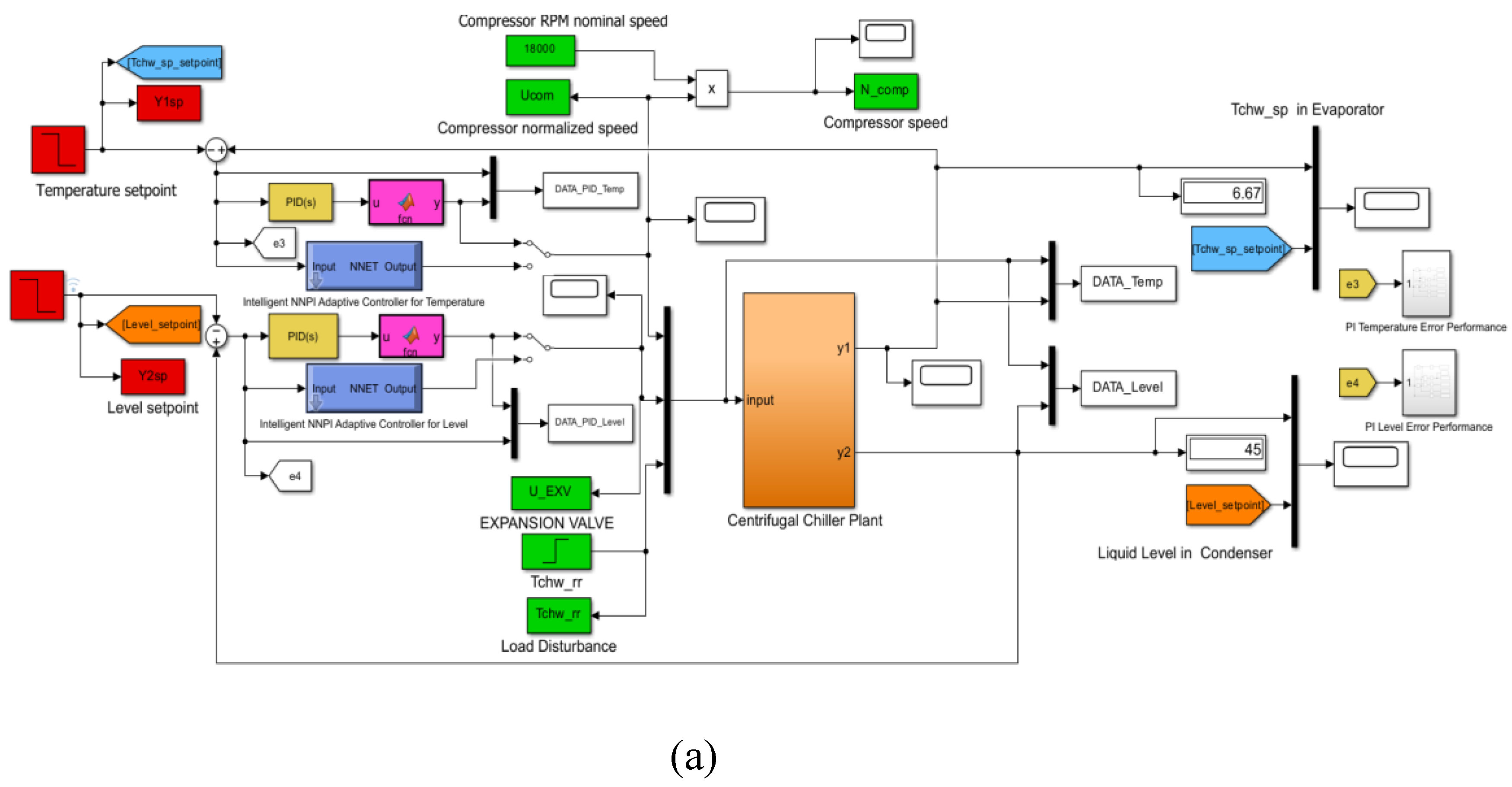
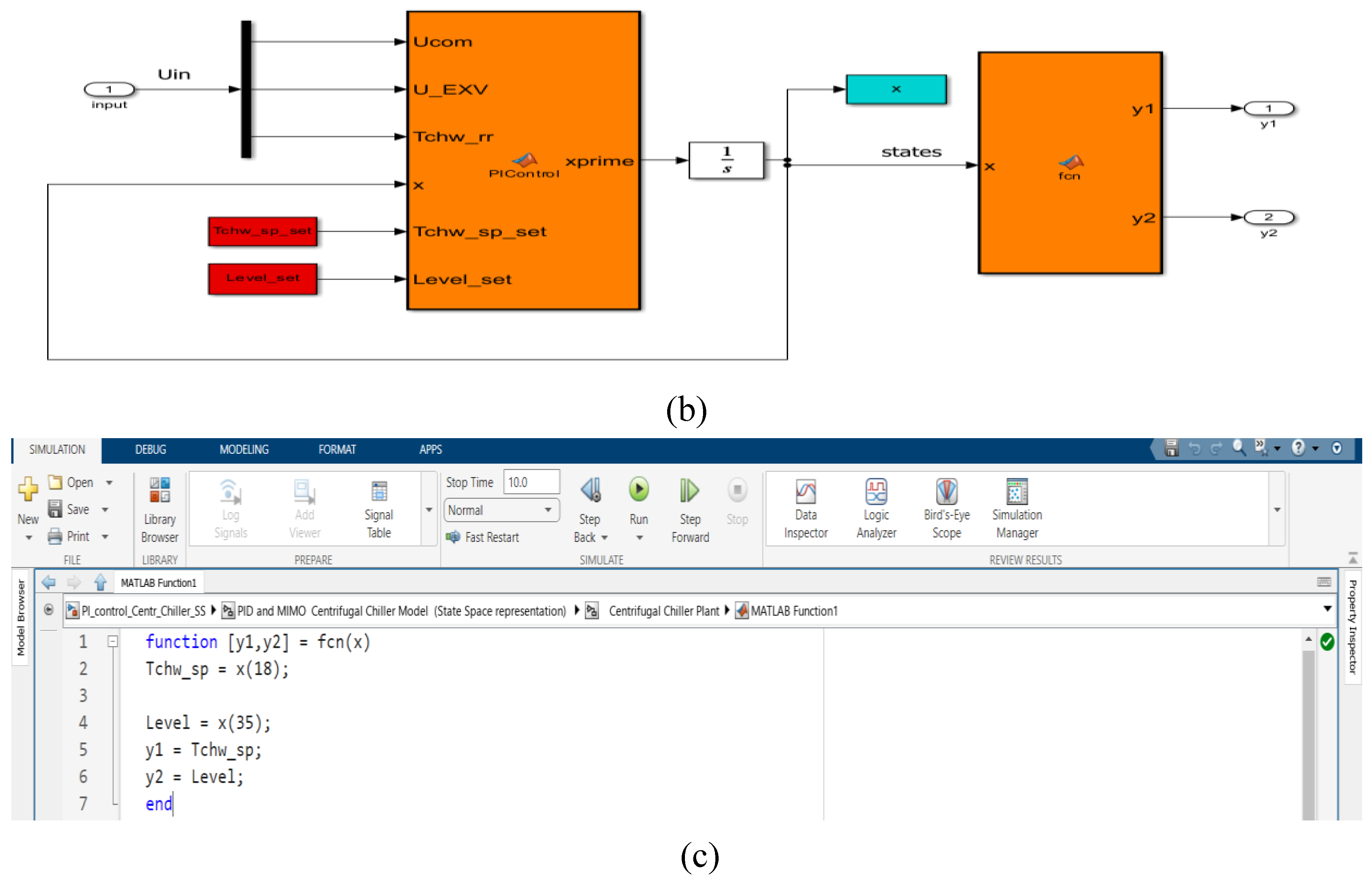
Figure A4.
PID ANFIS discrete-time simulation results -Rejection Temperature disturbance Tchw_rr. (a) Chilled water temperature inside Evaporator; (b) Liquid refrigerant level within Condenser.
Figure A4.
PID ANFIS discrete-time simulation results -Rejection Temperature disturbance Tchw_rr. (a) Chilled water temperature inside Evaporator; (b) Liquid refrigerant level within Condenser.
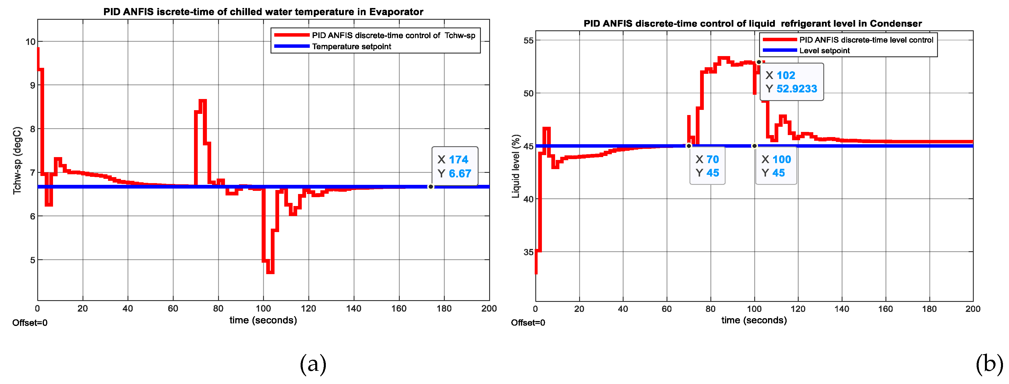
Figure A5.
PID ANFIS discrete-time control - MATLAB Simulink simulation results of actuators control efforts. (a) Compressor relative speed; (b)Expansion valve opening.
Figure A5.
PID ANFIS discrete-time control - MATLAB Simulink simulation results of actuators control efforts. (a) Compressor relative speed; (b)Expansion valve opening.
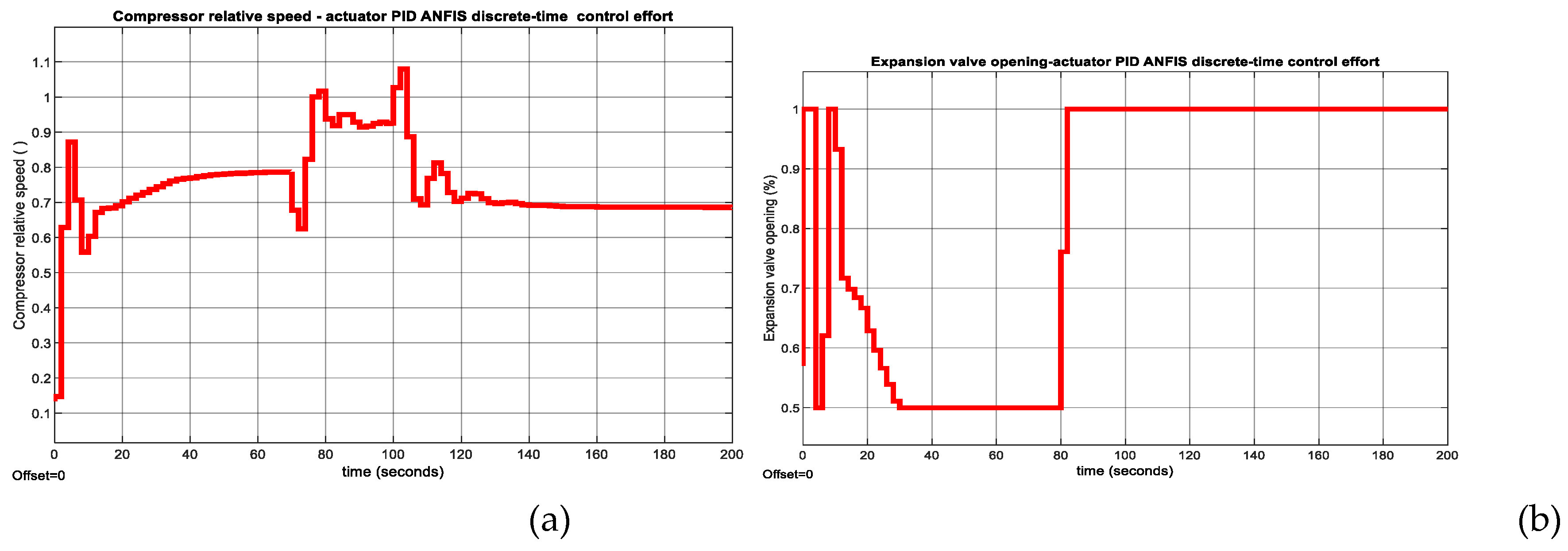
Figure A6.
PID ANFIS discrete-time control – MATLAB Simulink simulation results. (a) Chilled water temperature within Evaporator; (b) Liquid Refrigerant Level inside Condenser.
Figure A6.
PID ANFIS discrete-time control – MATLAB Simulink simulation results. (a) Chilled water temperature within Evaporator; (b) Liquid Refrigerant Level inside Condenser.
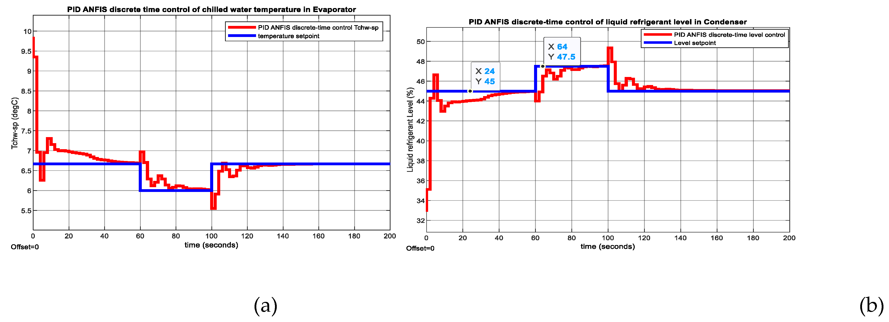
Figure A7.
PID ANFIS discrete-time control - MATLAB Simulink simulation results of actuators control efforts. (a) Compressor relative speed; (b)Expansion valve opening .
Figure A7.
PID ANFIS discrete-time control - MATLAB Simulink simulation results of actuators control efforts. (a) Compressor relative speed; (b)Expansion valve opening .
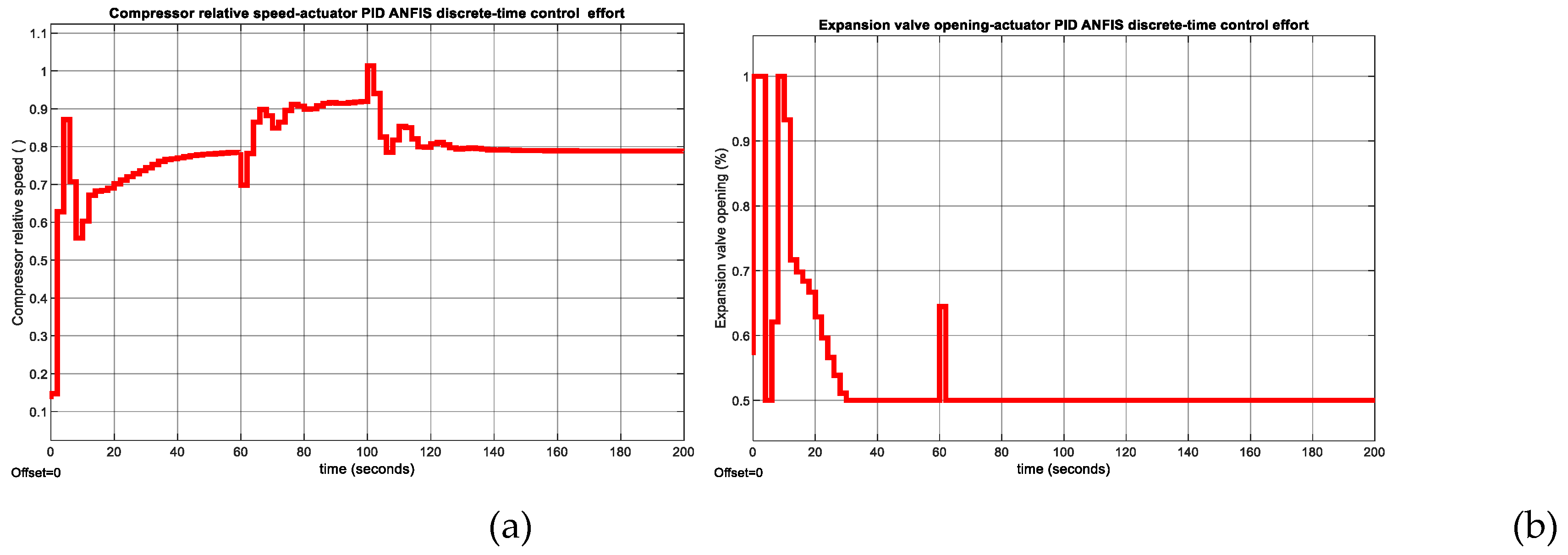
Figure A8.
The Data Statistics tables. (a) mpc Evaporator Temperature control; (b) RL DLNN Evaporator Temperature contrrol; (c ) mpc Condenser Refrigerant Level control; ( d) RL DLNN mpc Condenser Refrigerant Level control.
Figure A8.
The Data Statistics tables. (a) mpc Evaporator Temperature control; (b) RL DLNN Evaporator Temperature contrrol; (c ) mpc Condenser Refrigerant Level control; ( d) RL DLNN mpc Condenser Refrigerant Level control.
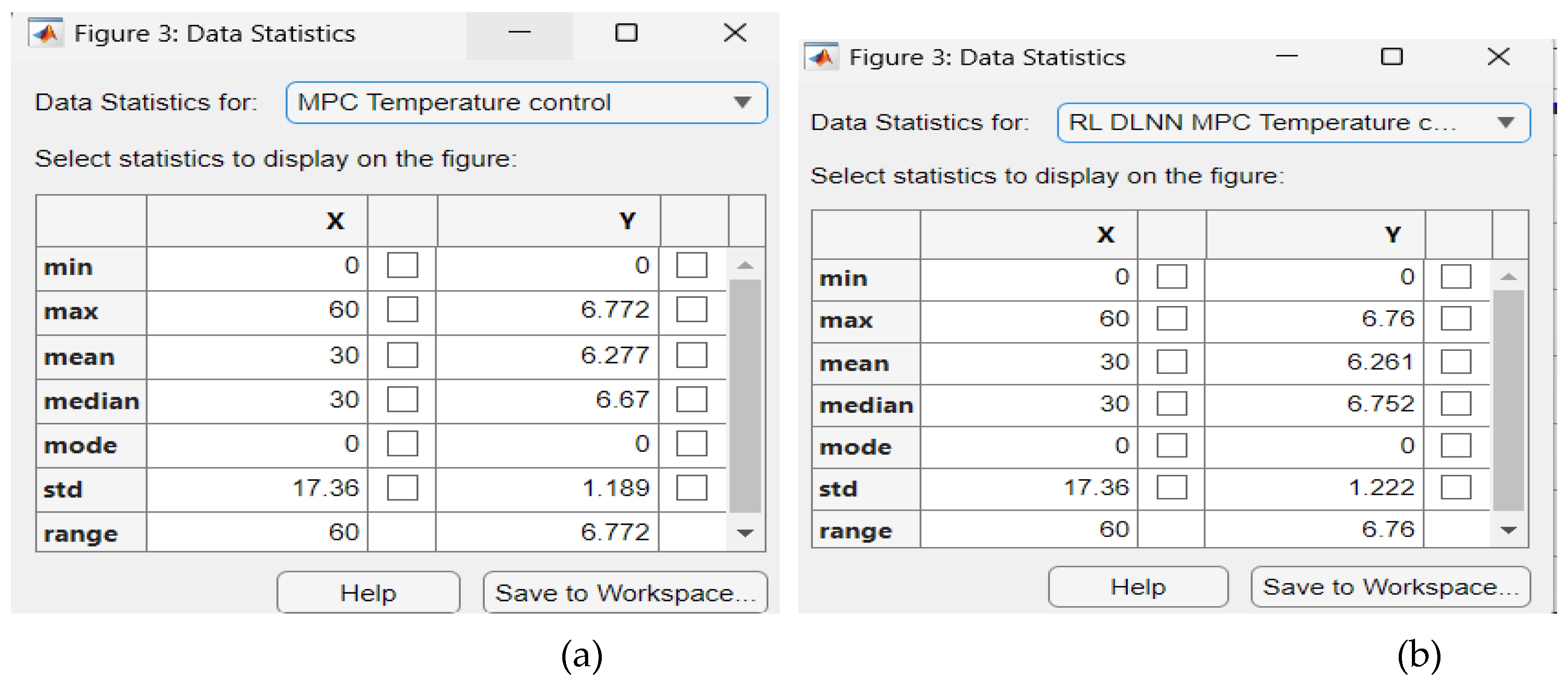
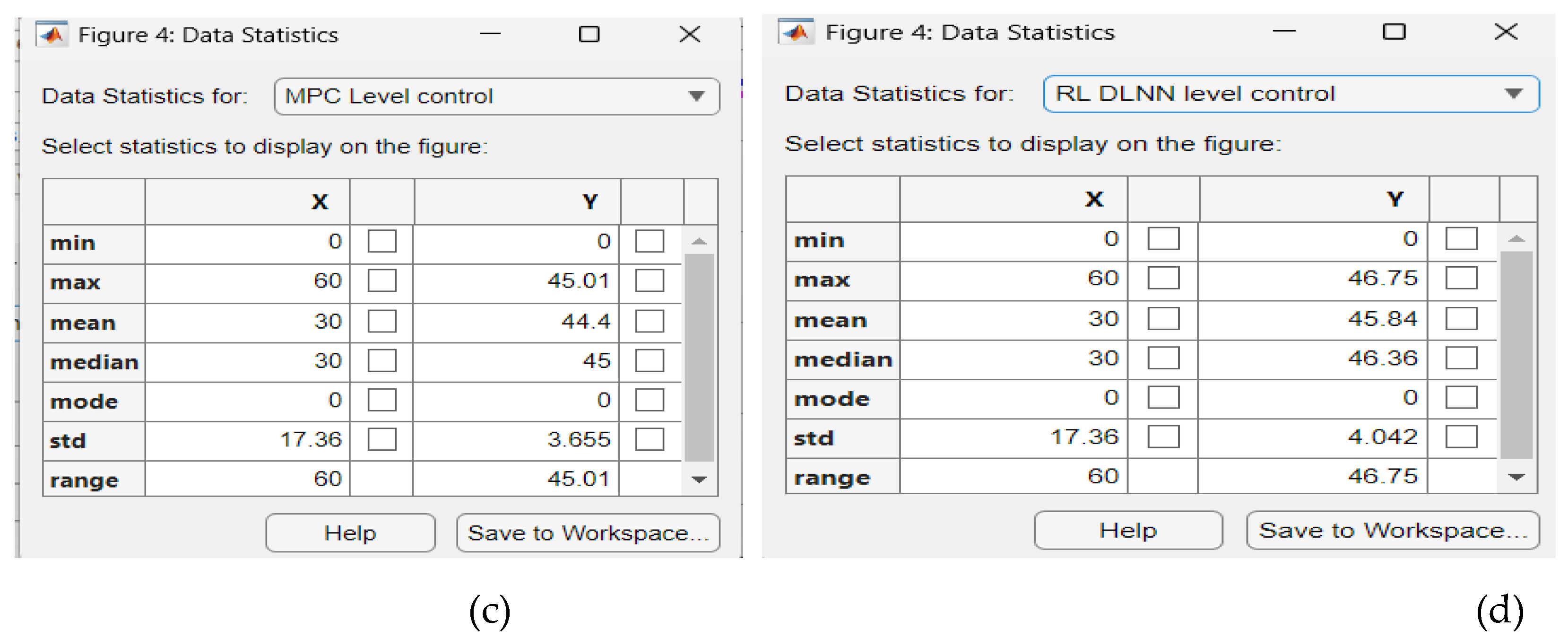
Figure A9.
Performance error indicators. (a) mpc Evaporator Temperature control; (b) RL DLNN Evaporator Temperature contrrol; (c ) mpc Condenser Refrigerant Level control; ( d) RL DLNN mpc Condenser Refrigerant Level control.
Figure A9.
Performance error indicators. (a) mpc Evaporator Temperature control; (b) RL DLNN Evaporator Temperature contrrol; (c ) mpc Condenser Refrigerant Level control; ( d) RL DLNN mpc Condenser Refrigerant Level control.
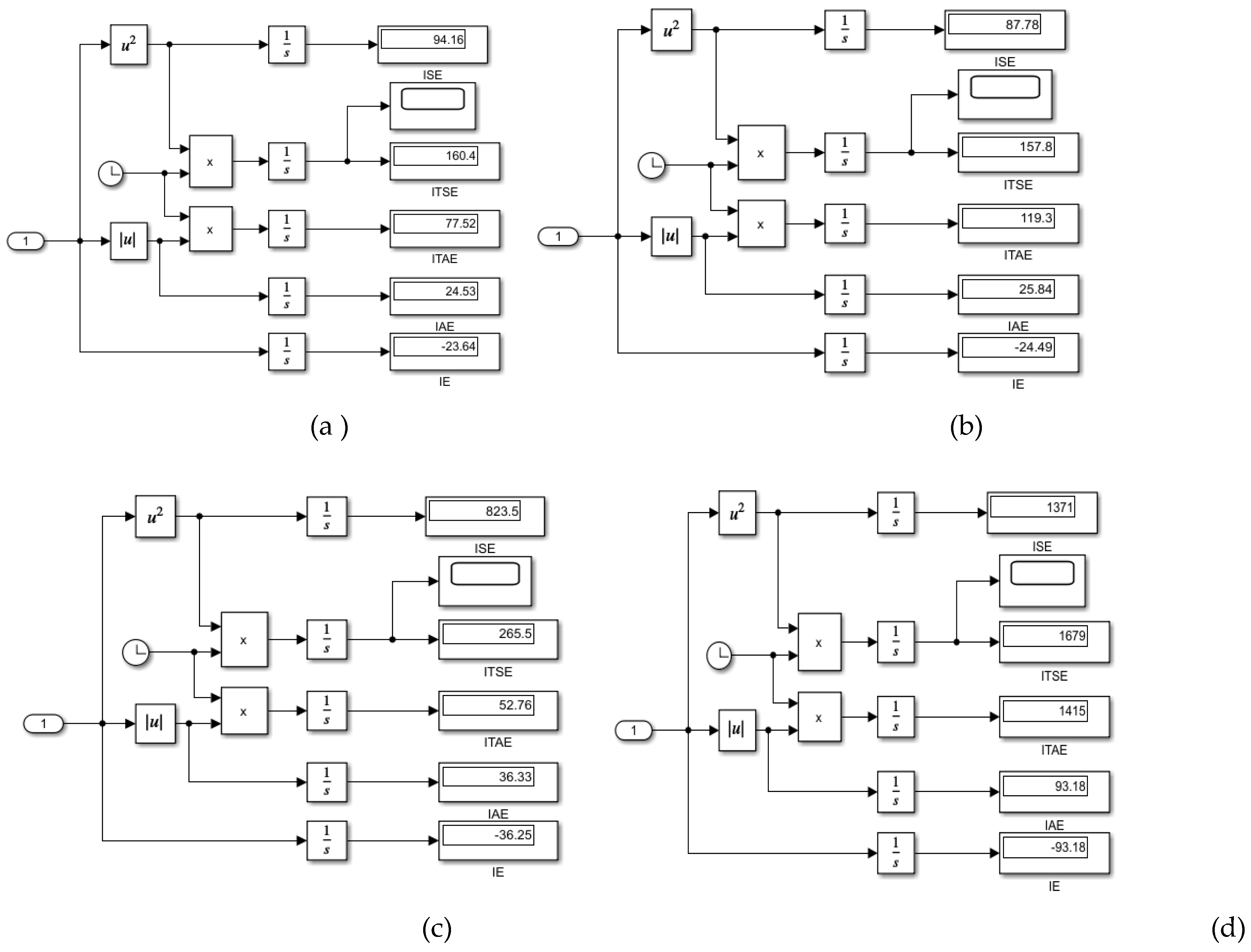
Figure A10.
The Data Statistics tables. (a) RL DLNN Evaporator Temperature contrrol; (b) Digital PID Evaporator Temperature control- CCS ANFIS model; (c RL DLNN mpc Condenser Refrigerant Level control;(d) Digital PID Condenser Refrigerant Level control - CCS ANFIS model.
Figure A10.
The Data Statistics tables. (a) RL DLNN Evaporator Temperature contrrol; (b) Digital PID Evaporator Temperature control- CCS ANFIS model; (c RL DLNN mpc Condenser Refrigerant Level control;(d) Digital PID Condenser Refrigerant Level control - CCS ANFIS model.
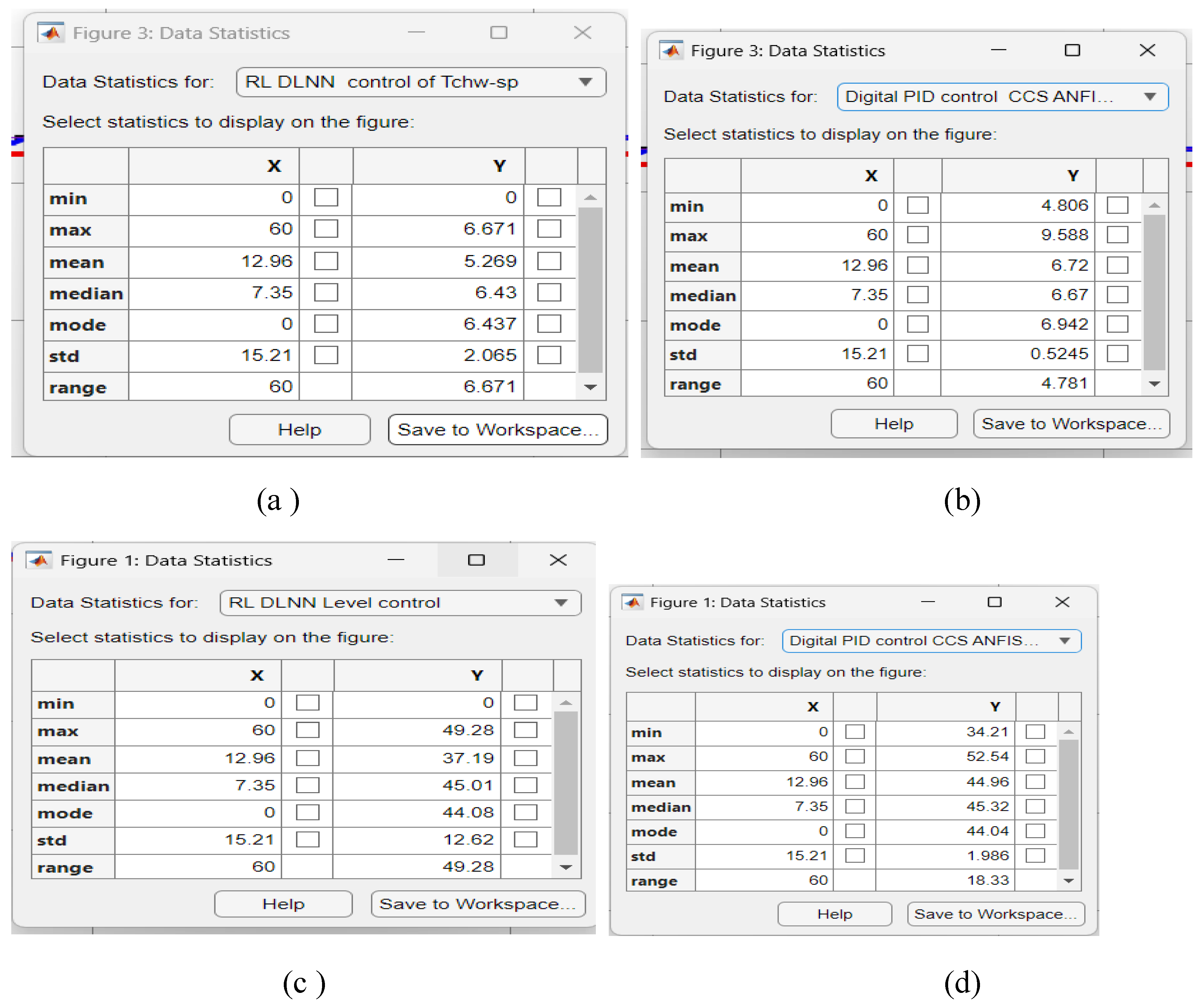
Figure A11.
Peerformance control error indicators. (a) RL DLNN Evaporator Temperature contrrol; (b) Digital PID Evaporator Temperature control- CCS ANFIS model; (c) RL DLNN Condenser Refrigerant Level control;(d) Digital PID Condenser Refrigerant Level control - CCS ANFIS model.
Figure A11.
Peerformance control error indicators. (a) RL DLNN Evaporator Temperature contrrol; (b) Digital PID Evaporator Temperature control- CCS ANFIS model; (c) RL DLNN Condenser Refrigerant Level control;(d) Digital PID Condenser Refrigerant Level control - CCS ANFIS model.
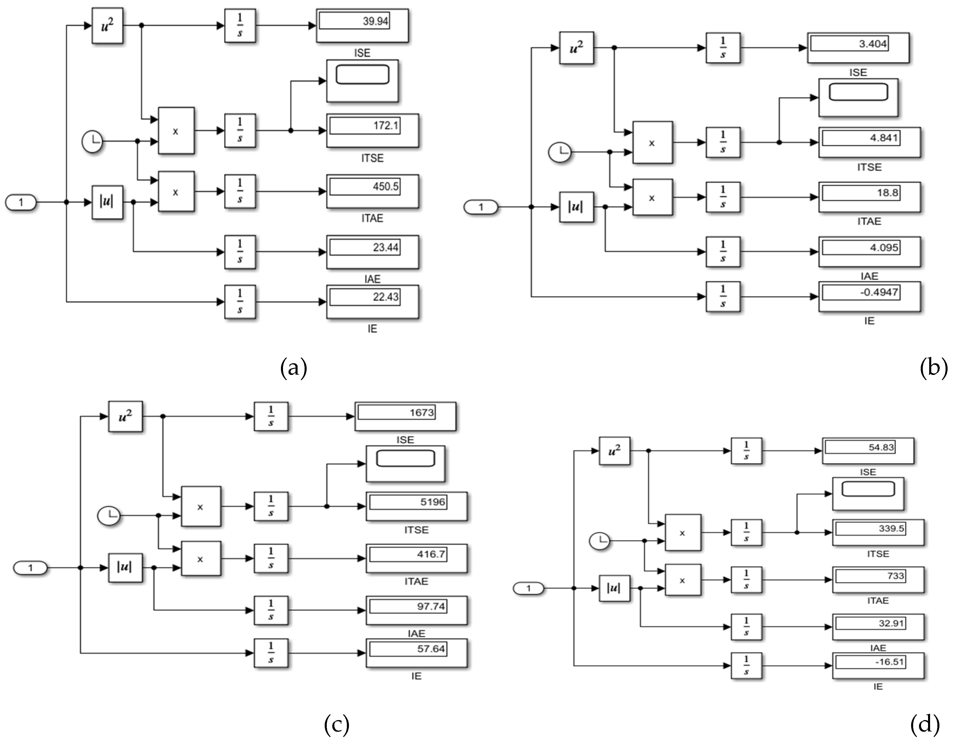
References
- Pengfei Li; Yaoyu Li; Seem, J.E. Modelica Based Dynamic Modeling of Water-Cooled Centrifugal Chillers. In: International Refrigeration and Air Conditioning Conference, Purdue University, July 12-15, 2010, pp.1-8. https://docs.lib.purdue.edu/iracc/1091.
- Pengfei Li; Yaoyu Li; Seem, J.E. et al. Recent advances in dynamic modeling of HVAC equipment. Part 2: Modelica – based modelling, Journal of HVAC&R Research, 20 (1), 2014, pp. 150-16.
- Gordon, J.M. Ng, K.C.; Chua, H.T. Centrifugal chillers: Thermodynamic modelling and a diagnostic case study, Int. J. Ref., 18 (4), 1995, pp.253-257.
- Popovic, P.; Shapiro, H. N. Modeling Study of a Centrifugal Compressor. In: ASHRAE Trans, Vol.104, Pt.2, Toronto, CA, 1998.
- Ning, M. Neural Network Based Optimal Control of HVAC&R Systems. PhD thesis, Department of Building, Civil and Environmental Engineering, Concordia University, Montreal, Quebec, 2008.
- Dhar, M.; Soedel W. Transient Analysis of a Vapor Compression Refrigeration System: Part I-The mathematical model. In: The XV-th International Congress of Refrigeration, Venice, 1979, pp.1035-1048.
- Wong S.P.W.; Wang, S.K. System Simulation of the performance of a Centrifugal chiller Using a Shell-and-Tube-Type Water-Cooled Condenser and R-11 as Refrigerant. ASHRAE Transaction, 1989, pp.445-454.
- Yu, F.W; Chan, K.T. Improved Condenser Design and Condenser-Fan Operation for Air-Cooled Chillers. In: Applied Energy, Vol. 83, 2006, pp. 628-648. [CrossRef]
- Wang, H. A steady-state empirical model for evaluating energy efficient performance of centrifugal water chillers, Energy and Buildings, Elsevier, 154, 2017, pp.415-419. [CrossRef]
- Wang, S.; Wang, J.; Burnet, J. Mechanistic Model of a Centrifugal Chiller to Study HVAC Dynamics. In: Building Services Engineering Research and Technology, Vol. 21(2), May 2000, pp. 73-83. [CrossRef]
- Beyene, A.; Guven, H.; et al. Conventional Chiller Performances Simulation and Field Data. In: International Journal of Energy Research, Vol. 18, 1994, pp. 391-399. [CrossRef]
- Braun, J.E.; Mitchell, J.W.; et al. Models for Variable-Speed Centrifugal Chillers. New York, NY, USA, ASHRAE, 1987.
- Browne, M.W.; Bansal, P.K. Steady-State Model of Centrifugal Liquid Chillers. In: International Journal of Refrigeration, 21(5), 1998, pp. 343-358. [CrossRef]
- 14. Songchun Li; Zaheeruddin, M. A Model and Multi-Mode Control of a Centrifugal Chiller System: A Computer Simulation Study, International Journal of Air-Conditioning and Refrigeration, Vol. 27, No. 4, 2019. [CrossRef]
- Tudoroiu, N.; Zaheeruddin, M.; Songchun Li; Tudoroiu, R-E. Design and Implementation of Closed-loop PI Control Strategies in Real-time MATLAB Simulation Environment for Nonlinear and Linear ARMAX Models of HVAC Centrifugal Chiller Control Systems. In Adv. Sci. Technol. Eng. Syst. J., Vol. 3(2), 25 April 2018, pp. 283-308. [CrossRef]
- Tudoroiu, R-E; Zaheeruddin, M.; Radu, S.M.; Budescu, D.D.; Tudoroiu, N. Design and Implementation in a New Approach of Non-minimal State Space Representation of a MIMO Model Predictive Control Strategy-Case Study and Performance Analysis. In: Advances in Artificial Intelligence-based Technologies. Learning and Analytics in Intelligent Systems, Vol. 22. Edited by: Virvou, M., Tsihrintzis, G.A., Tsoukalas, L.H., Jain, L.C., Springer, Cham, 03 October 2021. [CrossRef]
- Tudoroiu, N.; Zaheeruddin, M.; Tudoroiu, R-E; Modelling, identification, implementation and MATLAB simulations of multi-input multi-output proportional integral-plus control strategies for a centrifugal chiller system. In: International Journal of Modelling, Identification and Control (IJMIC), Vol.35 (1), February 24, Publisher: InderScience Online, London, UK, 2020, pp. 64-92.
- Ljung, L. System Identification Toolbox Getting Started Guide. The MathWorks, Inc.,1 Apple Hill Drive Natick, MA 01760-2098 © COPYRIGHT 1988–2023 by The MathWorks, Inc., MATLAB R2023a. Available online at: chrome-extension://efaidnbmnnnibpcajpcglclefindmkaj/https://control.dii.unisi.it/sysid/book/ident_gs.pdf (accessed on 12 June 2024).
- Landau, I.D.; Lozano, R.; M’Saad, M.; Karimi, A. Discrete-Time System Models for Control-Chapter 2. In: Adaptive Control, Communications and Control Engineering, Springer-Verlag London Limited, 2011, pp. 35-53.
- Ayman A. Nada; Shaban, E.M. The Development of Proportional-Integral-Plus Control Using Field Programmable Gate Array Technology Applied to Mechatronics System. In: American Journal of Research Communication, Vol. 2 (4), 2014, pp.14-27.
- Shaban, E.M.; Ayman A. Nada. Proportional Integral Derivative versus Proportional Integral plus Control Applied to Mobile Robotic System. In: Journal of American Science, Vol. 9 (12), 2013, pp. 583-591.
- Taylor, C.J.; Chotai, A.; Young, P.C. Proportional-integral-plus (PIP) control of time delay systems, Proceedings of the Institute Mechanical of Engineers, Vol. 212 (1), 1998, pp. 37-47. [CrossRef]
- Taylor, C.J.; Shaban, E.M. Multivariable Proportional-Integral-Plus (PIP) control of the ALSTOM nonlinear gasifier simulation. In: IEE Proceedings Control Theory and Applications, Vol. 153 (3), 2006, pp.277–285. [CrossRef]
- Young, P.C.; McCabe, A.P.; Chotai, A. State-dependent parameter nonlinear systems: Identification, Estimation and Control. In: IFAC, 15th Triennial World Congress, Barcelona, Spain, 2002. [CrossRef]
- Exadaktylos, V. Model Predictive Control Structures in the Non-Minimal State Space. PhD thesis, Lancaster University, UK, 2007.
- Ajith, A. Nature and Scope of AI Techniques. In: Handbook of Measuring System Design, edited by Peter H. Sydenham and Richard Thorn, John Wiley & Sons, Ltd., ISBN: 0-470-02143-8, 2005, pp.893-900.
- Bemporad, A.; Morari, M.; Ricker, N.L. Model Predictive Control Toolbox User’s Guide, The MathWorks, Inc., 2018, pp. 1-942. Available online at: https://www.mathworks.com/help/pdf_doc/mpc/mpc_ug.pdf.
- MathWorks MATLAB Version R2018b. Model Predictive Control Toolbox, On-line Documentation: https://www.mathworks.com/help/mpc/index.html.
- Zadeh, L.A. Fuzzy Sets, Fuzzy Logic, and Fuzzy Systems-Selected Papers by Lotfi Zadeh. In: Advances in Fuzzy Systems — Applications and Theory, Volume 6, , 840 pages. Edited By: George J Klir , Bo Yuan, State University of New York at Binghamton, USA, May 1996. [CrossRef]
- Haykin, S. Neural Networks and Learning Machines. 3rd ed. Eds: Marcia J. Horton, Dolores Mars, William Opaluch, Scott Disanno, Publisher: Pearson Education, Inc., Upper Saddle River, New Jersey 07458, 2009.
- Zurada, J.M. Introduction to Artificial Neural Systems.1st ed. Eds. Geri Davis, Quadrata, Loretta Palagi. Publisher: WEST PUBLISHING COMPANY 610 Opperman Drive P.O. Box 64526 St. Paul, MN 55164-0526, 1992.
- Tudoroiu, RE.; Zaheeruddin, M.; Radu, S.M.; Budescu, D.D.; Tudoroiu, N. The Implementation and the Design of a Hybrid digital PI Control Strategy Based on MISO Adaptive Neural Network Fuzzy Inference System Models–A MIMO Centrifugal Chiller Case Study. In: Tsihrintzis, G., Jain, L. (eds) Machine Learning Paradigms. Learning and Analytics in Intelligent Systems, Vol 18, Springer, Cham, 24 July, 2020. [CrossRef]
- Navneet Walia; Harsukhpreet Singh; Anurag Sharma. ANFIS: Adaptive Neuro-Fuzzy Inference System-A Survey. In: International Journal of Computer Applications (0975 – 8887), Volume 123, No.13, August 2015, pp.32-38.
- Jang R. ANFIS: Adaptive-Network-Based Fuzzy Inference System. In: IEEE Transactions on Systems, MAN, and Cybernetics, Vol. 23, No. 3, 1993. [CrossRef]
- Almabrok, A.; Psarakis, M.; Dounis, A. Fast Tuning of the PID Controller in An HVAC System Using the Big Bang–Big Crunch Algorithm and FPGA Technology. Algorithms 11, 146, 2018. [CrossRef]
- MathWorks Support Documentation-Help Center. Estimate ARMAX or ARMA model, Available online, URL: https://www.mathworks.com/help/ident/ref/armax.html (accessed on 12 June 2024).
- MathWorks Support Documentation-Help Center. Reinforcement Learning using Deep Neural Networks. Available online, URL: https://www.mathworks.com/help/deeplearning/ug/reinforcement-learning-using-deep-neural-networks.html (accessed on 10 September 2024).
- MathWorks Support Documentation-Help Center. Reinforcement Learning for Control Systems Applications. Available online, URL:https://www.mathworks.com/help/reinforcement-learning/ug/reinforcement-learning-for-control-systems-applications.html (accessed on 10 September 2024).
- MathWorks Support Documentation-Help Center. Generate Reward Function from a Model Predictive Controller for a Servomotor. Available online: https://www.mathworks.com/help/reinforcement-learning/ug/generate-reward-fcn-from-mpc-for-servomotor.html (accessed on 10 September 2024).
- MathWorks Support Documentation-Help Center. Generate Reward Function from a Model Verification Block for a Water Tank System. Available online: https://www.mathworks.com/help/reinforcement-learning/ug/generate-reward-fcn-from-verification-block-for-watertank.html(accessed on 20 September 2024).
- Kranthi Kumar, P.; Detroja, K.P. Design of Reinforcement Learning based PI controller for nonlinear Multivariable System. In: 2023 European Control Conference (ECC), Bucharest, Romania, 2023, pp. 1-6. [CrossRef]
- You, Weiyu; Yang, Genke; Chu, Jian; Ju, Changjiang. Deep reinforcement learning-based proportional–integral control for dual-active-bridge converter. Neural Computing and Applications, 35, 2023pp. 1-14. [CrossRef]
- MathWorks Support Documentation-Help Center. Resolving Low-Level Graphics Issues. Available online: https://www.mathworks.com/help/matlab/creating-plots/resolving-low-level-graphics-issues.html (accessed on 20 September 2024).
- Uzunovic, T.; Zunic, E.; Badnjevic, A.; Miokovic, I.; Konjicija, S. Implementation of digital PID controller, In: IEEE 33rd International Convention on Information and Communication Technology, Electronics and Microelectronics (MIPRO) , Vol. 33, Opatija, Croatia, May 2010, pp. 1357-1361.
Figure 1.
Chilled water flows through Centrifugal chiller subsystems, Evaporator and Condenser with all four main components (see [1,14]).
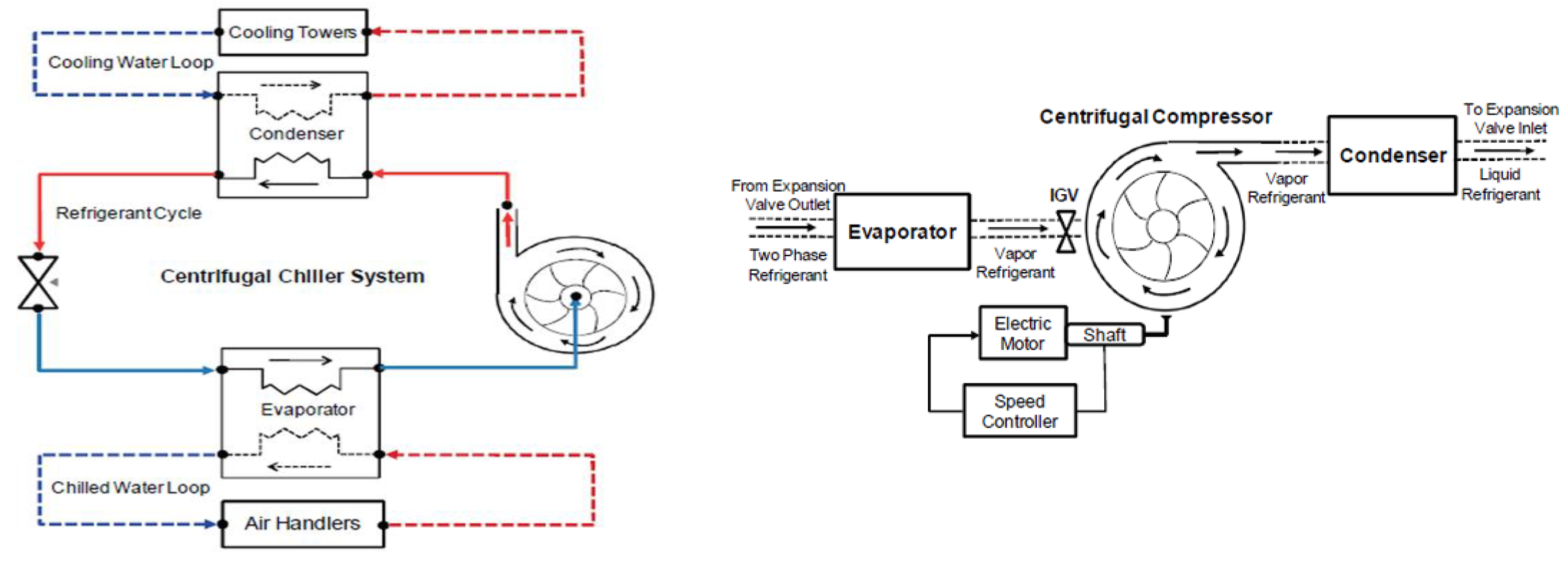
Figure 4.
Open loop linear simulation results for state-space MIMO ARMAX CCS model.
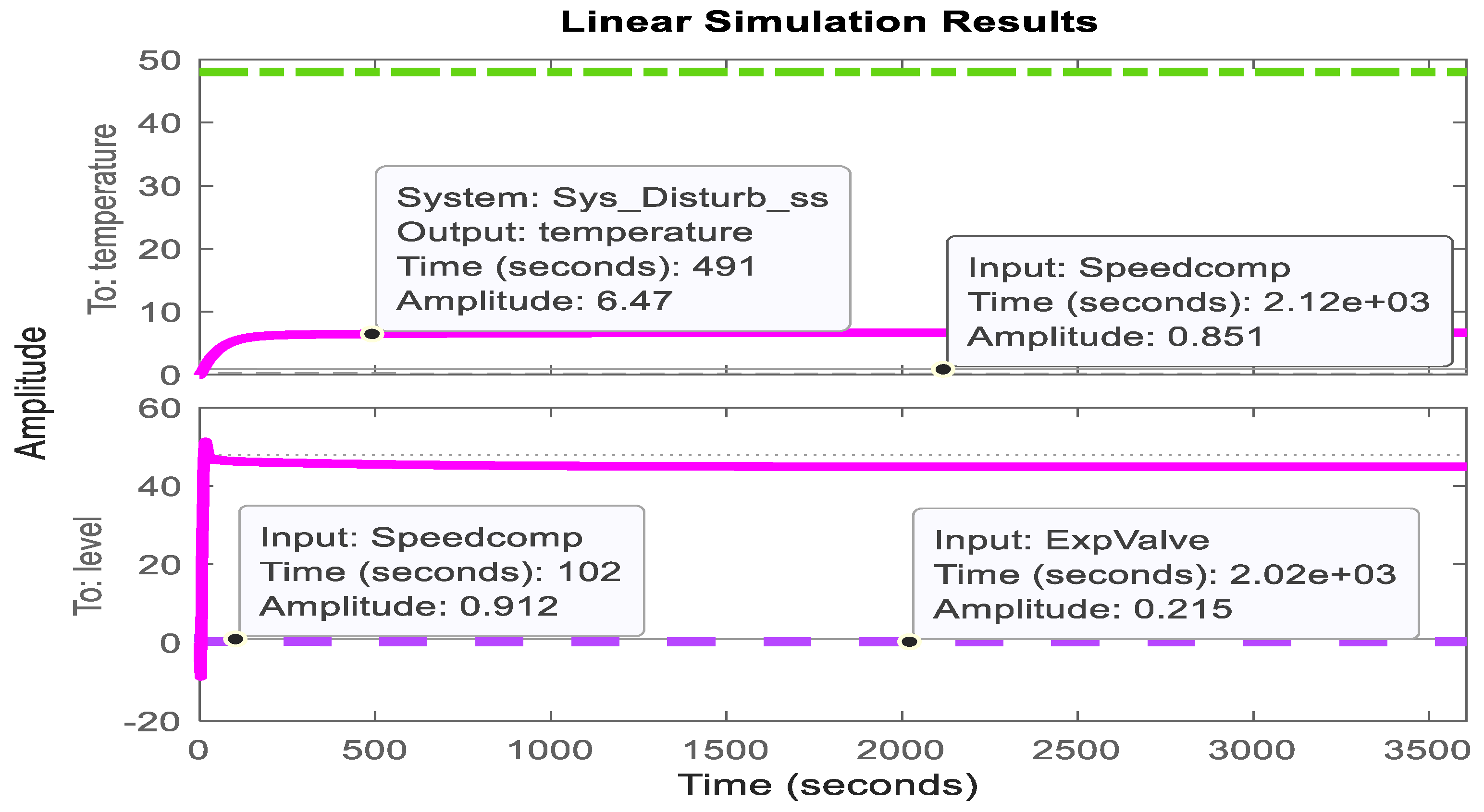
Figure 5.
Digital PID ANFIS discrete-time control temperature inside Evaporator and liquid refrigerant level within Condenser – overall Simulink diagram.
Figure 5.
Digital PID ANFIS discrete-time control temperature inside Evaporator and liquid refrigerant level within Condenser – overall Simulink diagram.
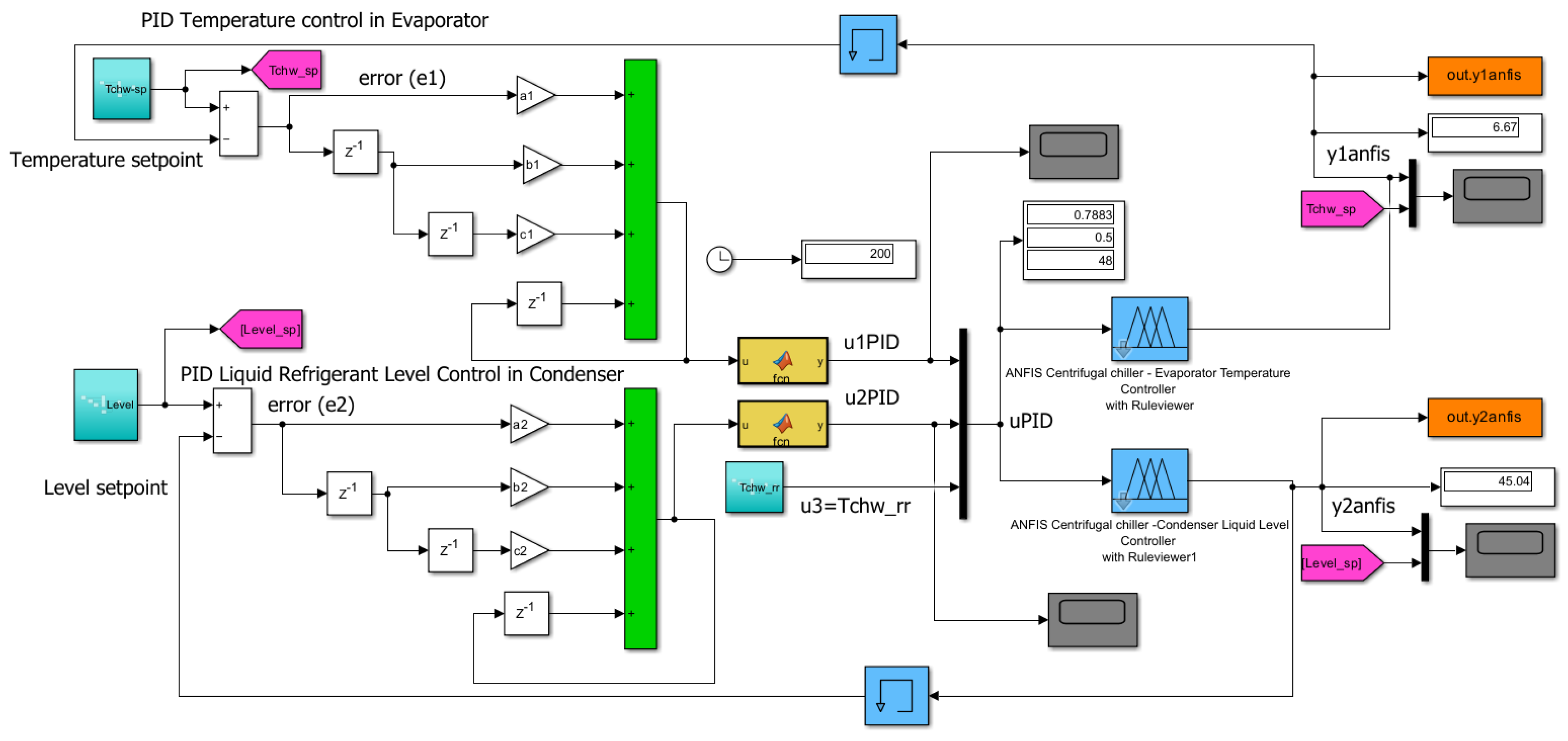
Figure 6.
Fuzzy Logic Designer application – MATLAB Simulink Simulation results; (a) Centrifugal Chiller FIS attached to temperature within Evaporator; (b) Centrifugal Chiller FIS membership functions; (c) Centrifugal Chiller FIS attached to temperature within Condenser; (d) Centrifugal Chiller FIS membership functions; (e) Chilled water Temperature within Evaporator training data and ANFIS model output estimation; (f) Liquid Refrigerant Level inside Condenser training data and ANFIS model output estimation; (g) Rule Viewer: fis MISO Chilled water temperature inside the Evaporater subsystem; (h) Rule Viewer: fis MISO Liquid refrigerant level within the Condenser subsystem.
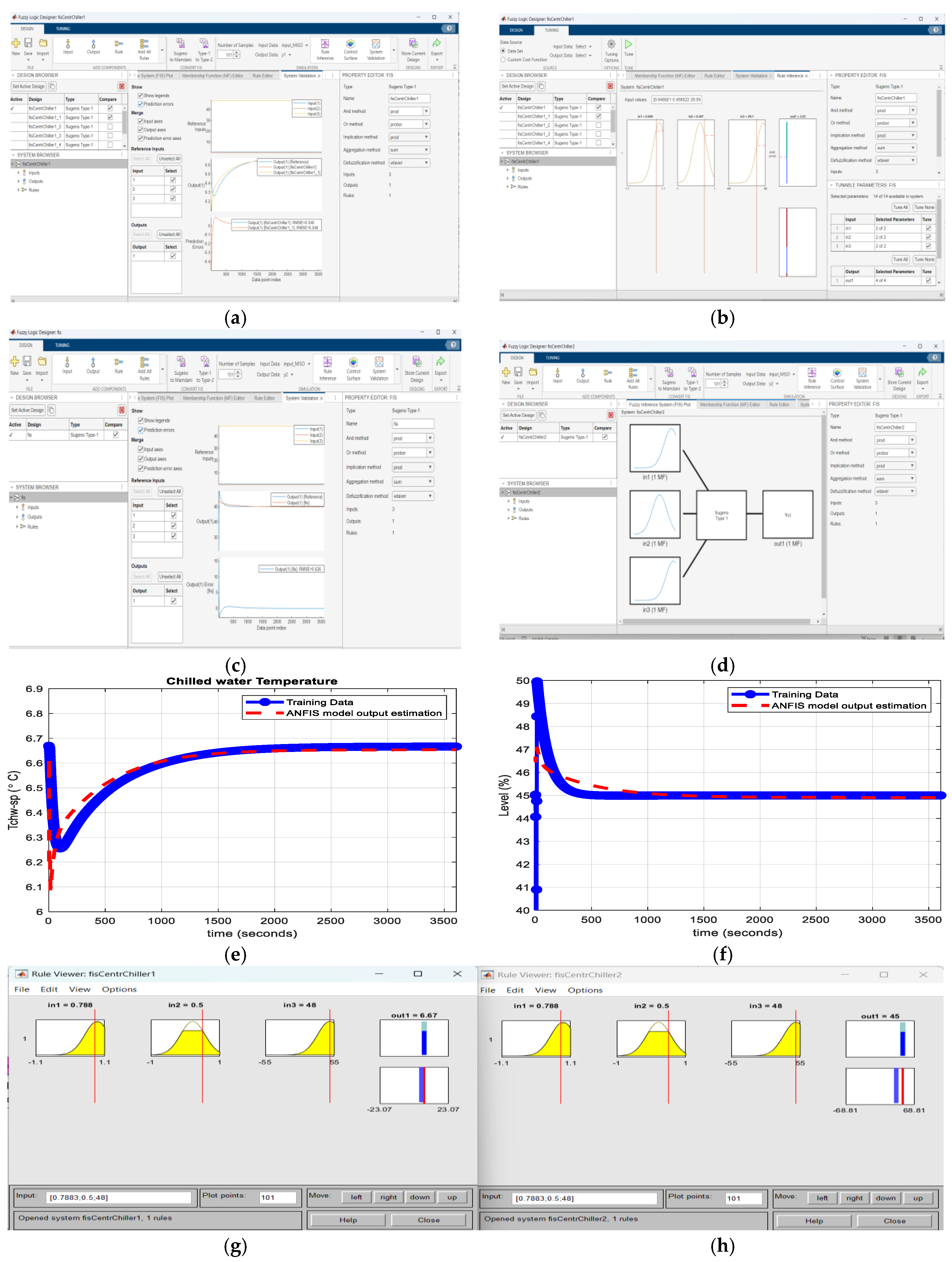
Figure 16.
MPC MATLAB Simulink simulations result in closed-loop for input (u1 =Ucom, u2=U-EXV, u3=Trr) and output (y1=Tch-sp, y2= Level) responses against internal plant using mpcDesigner application based on the input-output measurements dataset for MIMO CCS extended state model. (a) The actuators control efforts; (b) Temperature disturbance; (c) The chilled water Temperature in Evaporator; (d) The liquid refrigerant Level in Condenser; (e) MIMO centrifugal chiller model – mpc estimated states.
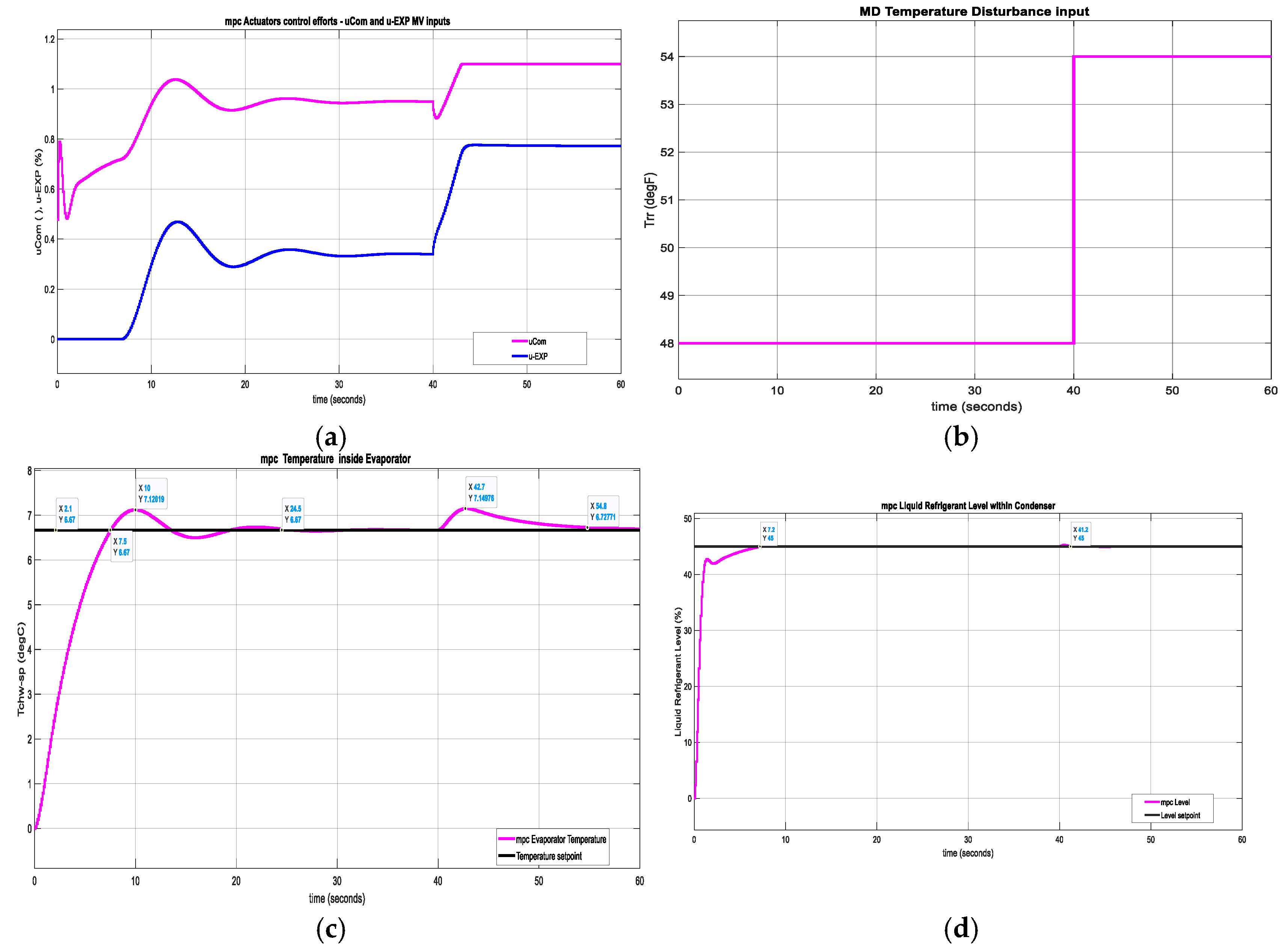
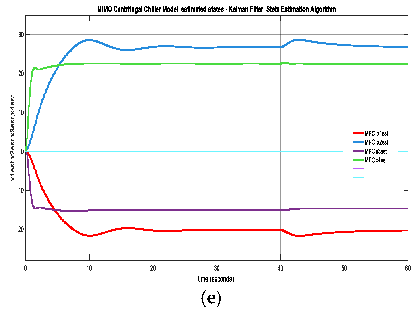
Figure 18.
MATLAB Simulink simulation results of RL DLNN versus Digital PID MIMO ANFIS model- Generate Reward Function from a step response specifications of MIMO Centrifugal Chiller simplified model in state space reprezentation. (a) RL DLNN of chilled water temperature inside the Evaporator versus Digital PID controller using ANFIS CCS models; (b) RL DLNN control of liquid Refrigerant level within the Condenser versus Digital PID controller using ANFIS CCS models; (c) Compressor actuator RL DLNN control effort; (d) Expansion Valve opening actuator RL DLNN control effort; (e) Compressor actuator Digital PID CCS ANFIS models control effort; (f) Expansion Valve opening actuator Digital PID CCS ANFIS models control effort.
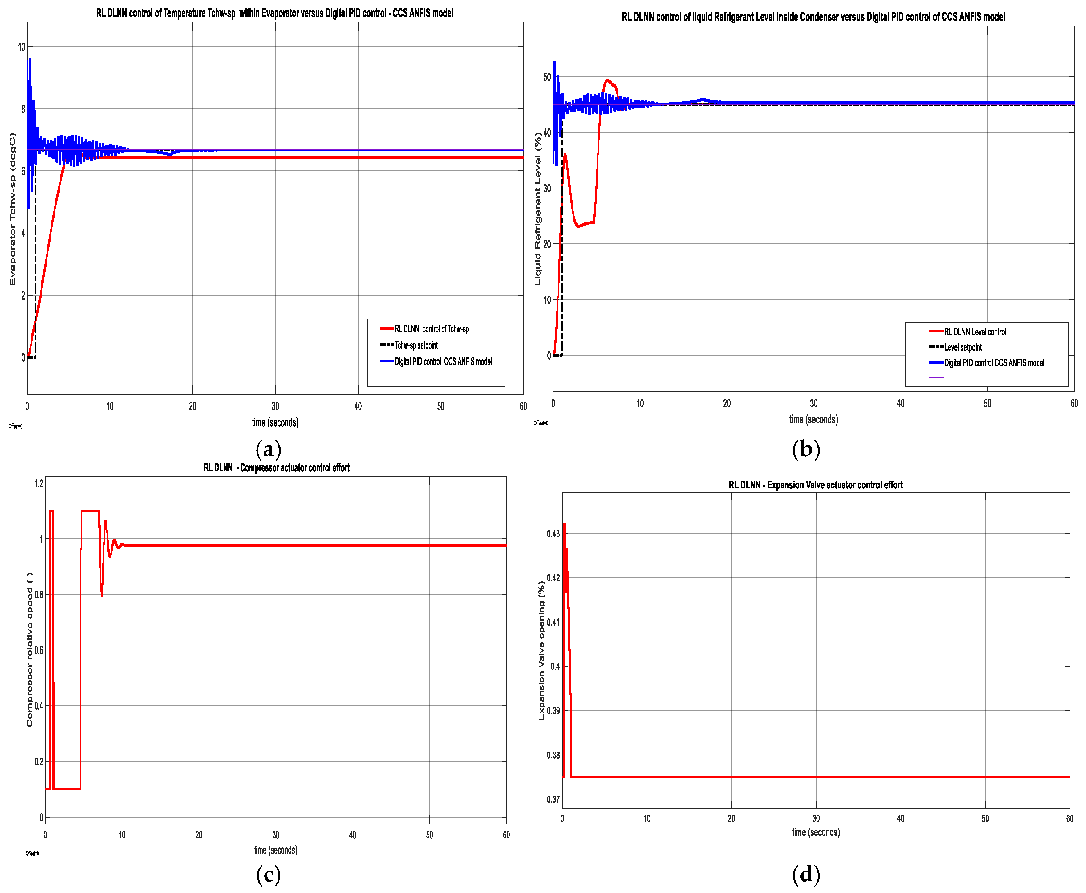
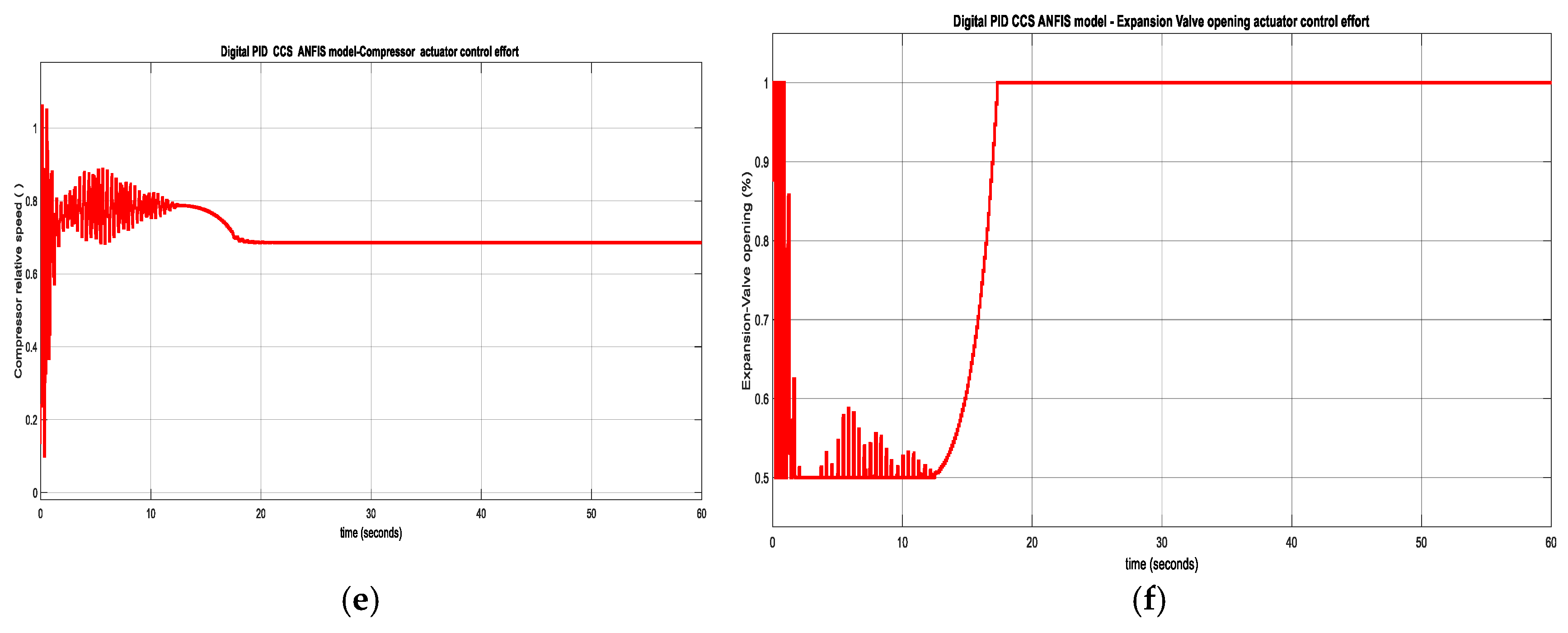
Figure 19.
Data Statistics extracted from the time responses. (a)TDI Evaporator Temperature control; (b) TDI Condenser Liquid Refrigerant Level control.
Figure 19.
Data Statistics extracted from the time responses. (a)TDI Evaporator Temperature control; (b) TDI Condenser Liquid Refrigerant Level control.
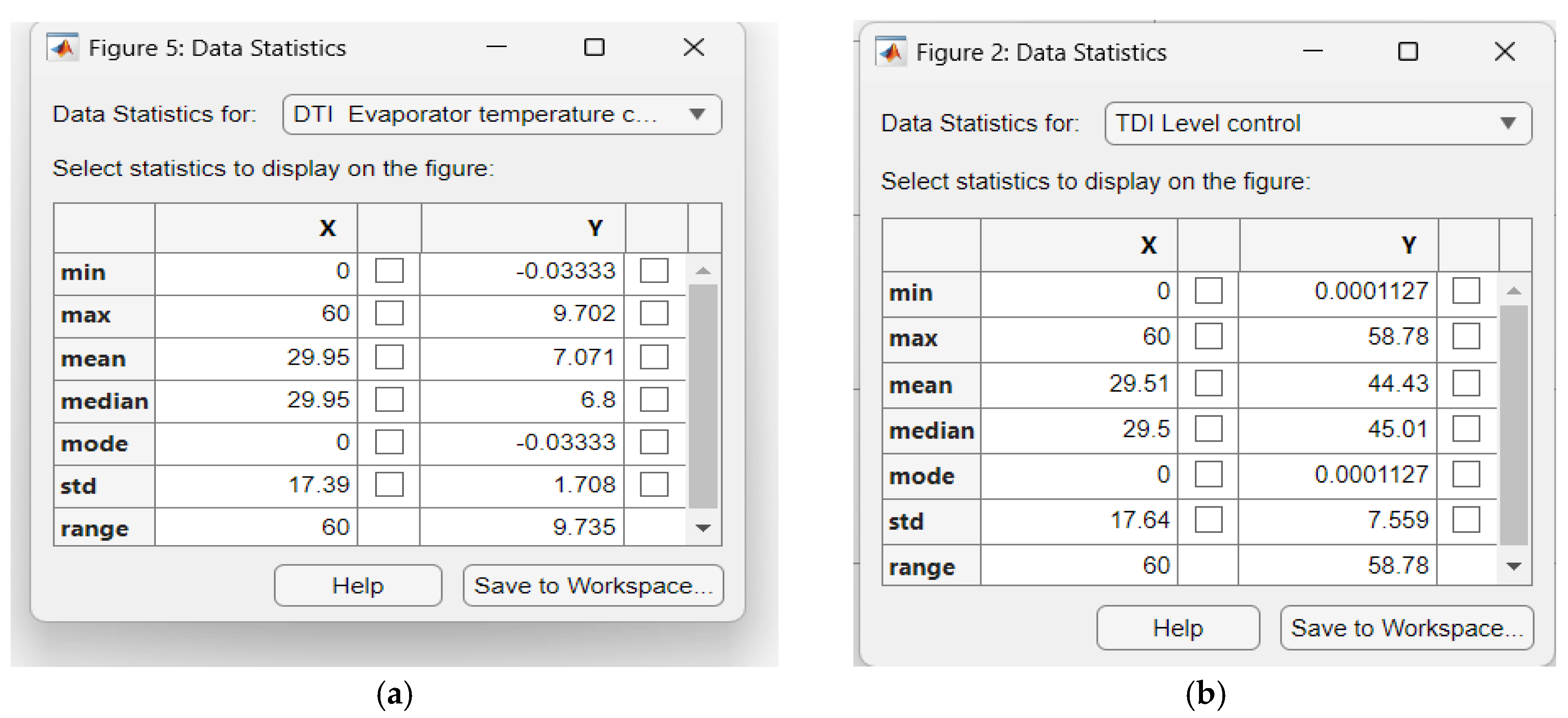
Figure 20.
Data Statistics extracted from the time responses. (a)PID Evaporator Temperature control; (b) PID Condenser liquid Refrigerant Level control.
Figure 20.
Data Statistics extracted from the time responses. (a)PID Evaporator Temperature control; (b) PID Condenser liquid Refrigerant Level control.
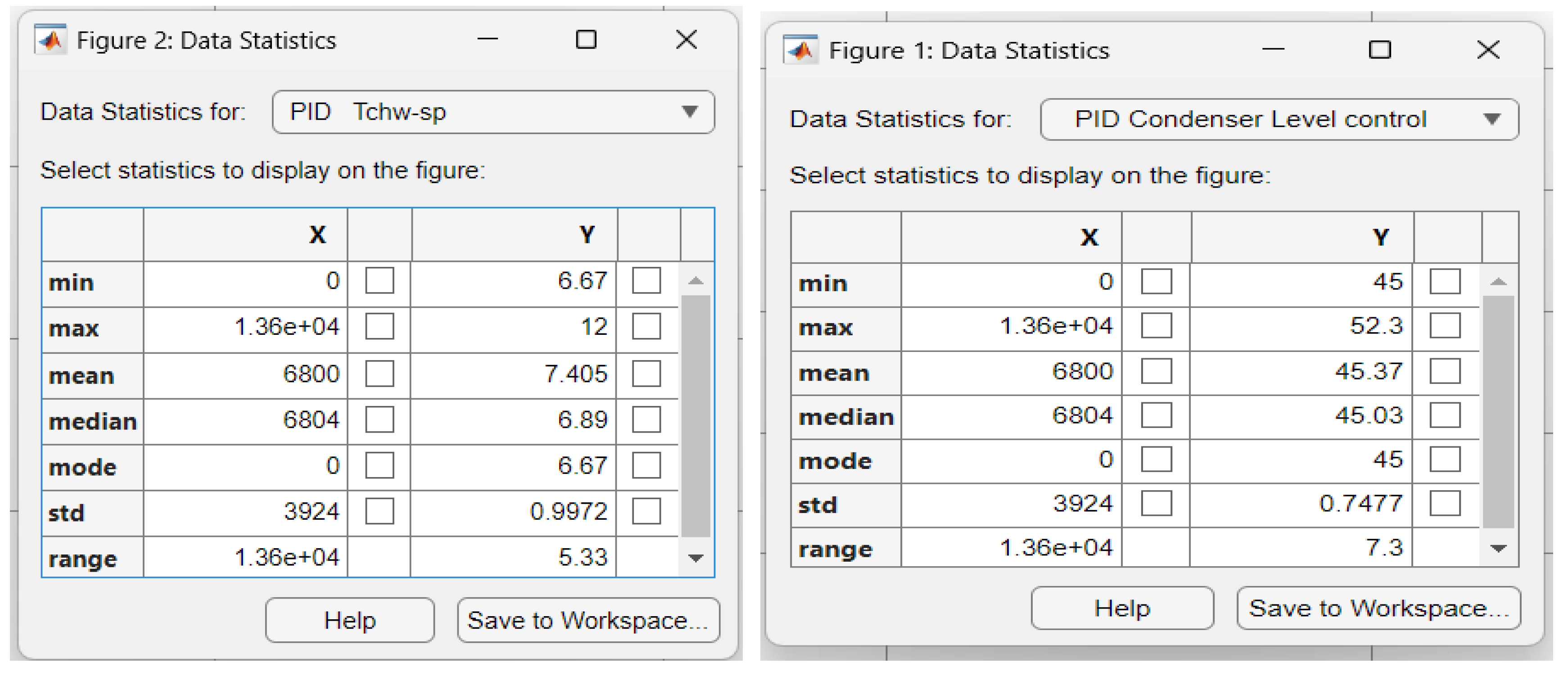
Disclaimer/Publisher’s Note: The statements, opinions and data contained in all publications are solely those of the individual author(s) and contributor(s) and not of MDPI and/or the editor(s). MDPI and/or the editor(s) disclaim responsibility for any injury to people or property resulting from any ideas, methods, instructions or products referred to in the content. |
© 2025 by the authors. Licensee MDPI, Basel, Switzerland. This article is an open access article distributed under the terms and conditions of the Creative Commons Attribution (CC BY) license (http://creativecommons.org/licenses/by/4.0/).
Copyright: This open access article is published under a Creative Commons CC BY 4.0 license, which permit the free download, distribution, and reuse, provided that the author and preprint are cited in any reuse.


