Submitted:
12 June 2024
Posted:
13 June 2024
You are already at the latest version
Abstract
The goal of the project was to understand how topography/bathymetry is imported and used in GeoFlood with an aim towards improving efficiency and computational cost of bathymetry handling in GeoFlood.GeoFlood is a software to simulate overland flooding basing on shallow water equations.Numerical methods and programming were used for this study.The GeoFlood was ran on a given data set (Malpasset data) and it was found out that indeed topography handling during simulations has to be improved to minimise the computational time and also improve the efficiency.Through this research, we also looked at the the shallow water equations, and the numerical techniques used to solve the equations
Keywords:
1. Bathymetry2. Shallow Water Equations3. Bilinear Integrals4. Piece Wise bilinear Surface
AN ESSAY PRESENTED TO AIMS RWANDA IN PARTIAL FULFILMENT OF THE REQUIREMENTS FOR THE AWARD OF MASTER OF SCIENCE IN MATHEMATICAL SCIENCES
1. Introduction
Typically, prior to conducting simulations, it is essential to first obtain or gather relevant data pertaining to the problem of interest. For our case we are interested in areas affected with floods, particularly overland flooding. Overland flooding refers to the situation where water levels rise and inundate typically dry land. This can be caused by various factors, including a river overflowing its banks, a storm surge from a hurricane, a significant amount of runoff from snow melt, or mechanical failures of dams or levees, among others. The high-risk areas for overland flooding include locations within floodplains, coastal regions, land near lakes, areas experiencing heavy seasonal rains, regions prone to frequent freeze-thaw cycles, and low-lying areas, including those below sea level. Therefore, the data in flood-affected areas is often referred to as either topography or bathymetry. Those two terms are distinct, yet their meanings overlap significantly. Topography encompasses surface features above sea level, such as mountains and buildings, while bathymetry pertains to features below sea level, such as rivers and lakes. In our project or within the code, our primary focus is on topography. Topography is usually collected from sources like Google map, Google earth and several other dedicated platforms for data collection.
Overland flooding leads to loss of lives, property damage, and hampers the development of affected areas.This research is dedicated to understanding and enhancing topography management within GeoFlood simulations, aiming to improve our understanding and prediction of overland flooding in complex environments.
Numerical simulation is a valuable tool for understanding and predicting overland flooding in complex environments. However, due to the extensive spatial domains and extended time frames overland flooding spans, it is essential to utilize suitable and manageable mathematical models to address this challenge. Models based on shallow water equations are commonly employed for this purpose, necessitating accurate representation of domain topography for precise modeling.
The computational costs associated with managing complex topography can be significant, espe- cially for models employing parallel adaptive mesh refinement (AMR) techniques like GeoFlood Kyanjo et al. (2024).To enhance computational efficiency and address computational cost chal- lenge, GeoFlood proposes a separate adaptive mesh for topography, which is then distributed to multiple processors using space-filling curve techniques, ensure that each processor points to a certain piece of the data and every time refinement or regrid happens, the required processor is just called.Additionally, new coupling features in P4est,the underlying mesh management library used in GeoFlood Burstedde et al. (2011), enable fast searches of a distributed P4est mesh or direct communication with the required processor.This approach effectively addresses the com- putational burden associated with handling topography, ensuring efficient simulation of overland flooding dynamics.
As discussed previously, to enhance efficiency and address computational cost during simulations in GeoFlood, we further need to think about grid cells within the computational domain, then compute their integrals.Since multiple topography files give us a digital description of the topog- raphy, we have to choose the finest(high resolution) level topography and then compute the area of ”reconstructed” numerical ”surface” over each grid cell.
The application to address the computational cost functions as the producer, with GeoFlood acting as the consumer utilizing the application.Upon regridding or refining, GeoFlood temporarily halts, triggering the application to generate integrals.Each processor computes these integrals and makes them accessible.Consequently, when either refined or coarser integrals are necessary, they can be swiftly referenced.Implementing this approach will markedly reduce simulation time.
The sections that will follow include, software packages used in GeoFlood during simulations, Overland flooding model, discussing shallow water equations to be solved during simulations and numerical techniques employed to solve them, methodology, to talk about how topography is handled in GeoFlood, results and discussions and conclusion.
2. Overland Flooding Modeling
In this chapter we are going to briefly discuss the numerical techniques that GeoFlood employs to solve the shallow water eqautions and the shallow water equations themselves.
2.1. Shallow Water Equations
Shallow water equations are a system of hyperbolic partial differential equations that govern the flow beneath a pressure surface in a fluid.These equations are derived from the principles of conservation of mass and momentum.These are nonlinear system of hyperbolic conservation laws for depth and momentum(LeVeque et al., 2011).In one space dimension, these take the form:
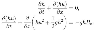
where
- g is the gravitational constant,
- h(x,t) is the fluid depth,
- u(x,t) is the vertically averaged horizontal fluid velocity.
A drag term D(h, u)u can be added to the momentum equation and is often important in very shallow water near the shoreline.
B(x) represents the bottom surface elevation relative to mean sea level.Negative values of B correspond to submarine bathymetry,while positive values indicate topography.
Figure 2.
1: Figure shows variables of shallow water equations (LeVeque et al., 2011).
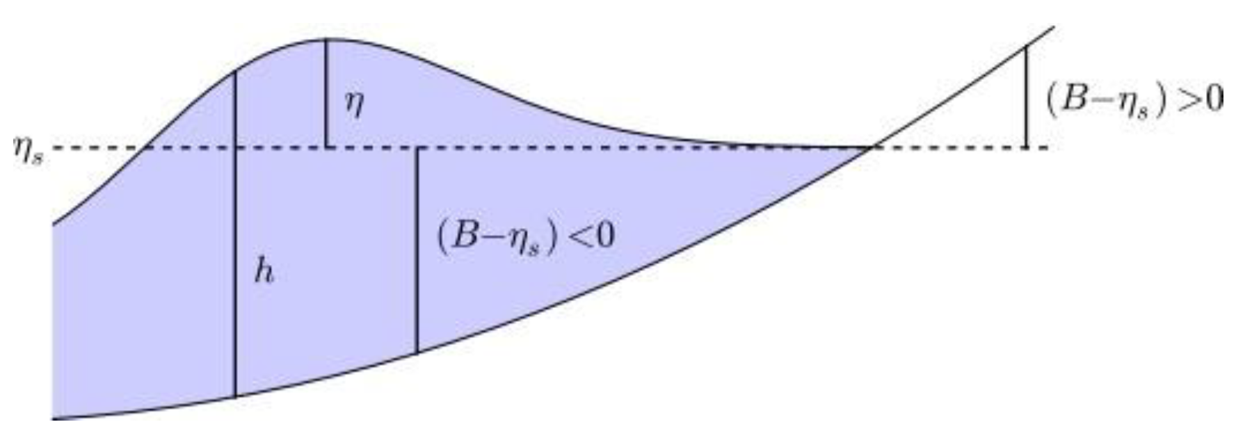
The equation for the water surface elevation is expressed as follows
η(x, t) = h(x, t) + B(x, t),
In two dimensions, the shallow water equations are formulated as follows:
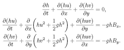
where
- u(x,y,t) and v(x,y,t) are the depth-averaged velocities in the two horizontal directions,
- B(x,y,t) is the topography.
Once more, a drag term could potentially be incorporated into the momentum equations.
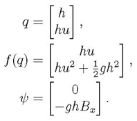
It is important to note that shallow water equations are part of the broader category of hyperbolic systems
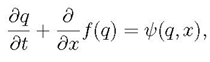
where
- q(x, t) is the vector of unknowns,
- f (q) is the vector of corresponding fluxes,
- ψ(q, x) is a vector of source terms.
These vectors can be represented mathematically as
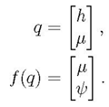
Let us introduce the notation µ = hu for momentum and ϕ = hu2 + 21 gh2 or momentum flux. Then, the momentum vector and momentum flux can be respectively rewritten as
The Jacobian matrix Jf then has the form
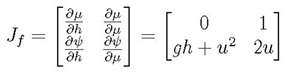
Hyperbolicity requires that the Jacobian matrix be diagonalizable with real eigenvalues and linearly independent eigenvectors.In the case of shallow water equations, the matrix Jf has
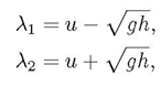 and corresponding
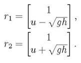
2.2. Finite Volume Technique to Solve Hyperbolic PDEs:
These numerical methods are appropriate for solving nonlinear hyperbolic systems such as the shallow water equations (LeVeque et al., 2011).In a one-dimensional finite volume method, the numerical solution Qi approximates the average value of the solution within the ith grid cell
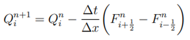
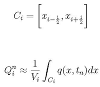 where Vi represents the volume of the grid cell, which is simply the region in one dimension,
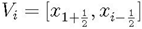
The wave propagation algorithm updates the numerical solution from  to
to  by solving Riemann problems at
  and
and  , the boundaries of Ci, and using the resulting wave structure of the Riemann problem to determine the numerical update.
to by solving Riemann problems at and , the boundaries of Ci, and using the resulting wave structure of the Riemann problem to determine the numerical update.For a homogeneous system of conservation laws, that is qt + f (q)x= 0, such methods are often written in conservation form
 where
where  is a numerical flux approximating the time average of the true flux across the left edge of cell Ci over the time interval. The expression of
  is defined as
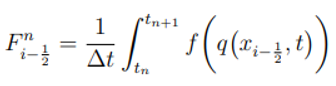
2.3. Riemann Solver
The process of creating a computational/mathematical representation of the area that will be affected by floods, mostly with highly variable and irregular topography is a bit complicated due to huge change in the flow of the floods over a distance and source terms resulting from variable topography.This issue becomes more intricate due to the existence of a solution domain that changes as a result of moving from wet to dry boundaries.To solve this issue, GeoFlood uses an approximate Riemann solver by (George, 2008) that solves an augmented shallow water equation system that includes the momentum flux and topographic bed in order to determine waves in the Riemann solver.They are used to compute the numerical flux across a discontinuity in the Riemann problem. Riemann solver provides an exact or approximate weak solution to the hyperbolic PDE given initial data that is a piece wise constant with a single jump discontinuity.
2.4. Adaptive Mesh Refinement
Adaptive mesh refinement (AMR) is a numerical method used for solving Partial Differential Equa- tions (PDEs).The computational domain, which encompasses the region surrounding the floods, is discretized into a uniform grid resolution based on the complexity of the solution.Initially, the computational domain is divided into a coarse grid with Uniform spacing to provide a basic approximation of the solution.Throughout the simulations, the local error of the solution is con- tinuously monitored using various techniques, such as comparing numerical solutions at different resolutions.
Refinement criteria by (George, 2006) are then applied based on the estimated error to identify regions of the domain where the solution requires higher resolution, particularly in regions affected by floods.These criteria may include:
Water Depth Criteria:In this context, refinement is only allowed in regions where cells contain water, achieved by flagging cells with water depths exceeding a certain threshold value.The refinement level is then determined based on the water depth.
Bathymetry flag:This criterion is employed to enforce refinement in shallow regions where flow dynamics change rapidly, such as near riverbanks or shorelines.
Velocity Criteria:This assume that the magnitude of the water velocity in both x and y directions is greater than a certain threshold value.
Flood Source Flags:This criterion is employed to enforce refinement in regions containing the flood source, such as a dam in the case of a dam break.It enables the code to refine the flood source at a high resolution to capture flood details along the floodplain.Moreover, it allows for the specification of regions to be refined to a desired resolution, determined by user-defined coordinates as well as minimum and maximum refinement levels.
Flow-grades flag:In this context, refinement is mandated to specified levels for depths or ve- locities surpassing user-defined thresholds.This functionality enables the code to refine regions containing lakes, seas, or rivers within the floodplain at varying intermediate levels compared to the flowing material.Note that refining involves increasing the resolution or level of detail in specific regions of the computational grid or mesh.
Mesh refinement is additionally conducted in regions where the solution necessitates higher res- olution (such as flood areas), while coarsening occurs where the solution is relatively smooth or less complex.After refining the mesh or grid, values from neighbouring grid cells are interpolated to compute the solution at the refined grid points.The solution is then updated using numerical methods like finite volume method.
The adaptive refinement process is iterative, with the solution evolving over time.Adaptive Mesh Refinement (AMR) improve the efficiency and accuracy of numerical simulations for hyperbolic PDEs by concentrating computational resources on regions where they are most needed, such as regions affected by floods.It is used for solving many other different PDEs, including parabolic and elliptic PDEs.
3. Software Packages Incorporated in GeoFlood
In this chapter we are briefly going to see some software libraries incorporated with in GeoFlood to perform simulations on overland flooding.GeoFlood is a new open-source software package designed for solving shallow water equations (SWE) on a quadtree hierarchy of mapped, logically Cartesian grids managed by the parallel adaptive library ForestClaw (Calhoun and Burstedde, 2017).As mentioned previously, GeoFlood utilizes ForestClaw and p4est to address specific chal- lenges in modeling overland flooding, which will be discussed further in this section.More about the installation and operation of GeoFlood is provided on the GeoFlood Wiki (Kyanjo, 2023) Additionally, this section briefly introduces another software called GeoClaw that is also designed to solve hyperbolic systems of partial differential equations, it is used to benchmark GeoFlood to evaluate its performance.
3.1. P4est
The p4est code serves as a robust parallel library tailored for adaptive hierarchical tree mesh par- allel computation.It offers effective parallel algorithms to facilitate the creation, refinement, and distribution of tree-based meshes.Through the p4est mesh management library, a quadtree or oc- tree mesh can be seamlessly distributed across multiple processors utilizing the Message-Passing Interface (MPI).This approach establishes a scalable and robust framework suitable for large-scale simulations, ensuring resilience against faults.Moreover, the design of p4est prioritizes compatibil- ity with diverse parallel computing architectures, enabling seamless scaling to encompass millions of processor cores.(Burstedde et al., 2011).
3.2. GeoClaw
GeoClaw software is a submodule of Clawpack (Mandli et al., 2016), an open-source software package designed for solving general hyperbolic systems of partial differential equations (PDEs) using finite-volume methods on logically Cartesian grids (George, 2006).GeoClaw integrates finite- volume wave propagation algorithms from Clawpack, Riemann solvers specifically designed for shallow water equations, patch-based Adaptive Mesh Refinement schemes tailored for free-surface flows over topography, and methods for ingesting and interpolating general sets of topography or bathymetry, which may be overlapping or nested.
3.3. ForestClaw
The ForestClaw library is built as a PDE layer on top of the p4est library, facilitating parallel tree mesh management.It is a forest-of-quadtrees approach to block structured adaptive mesh refinement.ForestClaw extensively utilizes the wave propagation algorithms in Clawpack to address various hyperbolic problems.Therefore, the resulting ForestClaw library emerges as an adaptive, parallel, multi-block structured finite volume code, enabling the parallelization of hyperbolic PDE solutions on mapped logically Cartesian meshes (Calhoun and Burstedde, 2017).
Figure 3.
1: Figure shows three 8 × 8 computational grids, each with a layer of ghost cells, at three adjacent levels. (Calhoun and Burstedde, 2017).
Figure 3.
1: Figure shows three 8 × 8 computational grids, each with a layer of ghost cells, at three adjacent levels. (Calhoun and Burstedde, 2017).
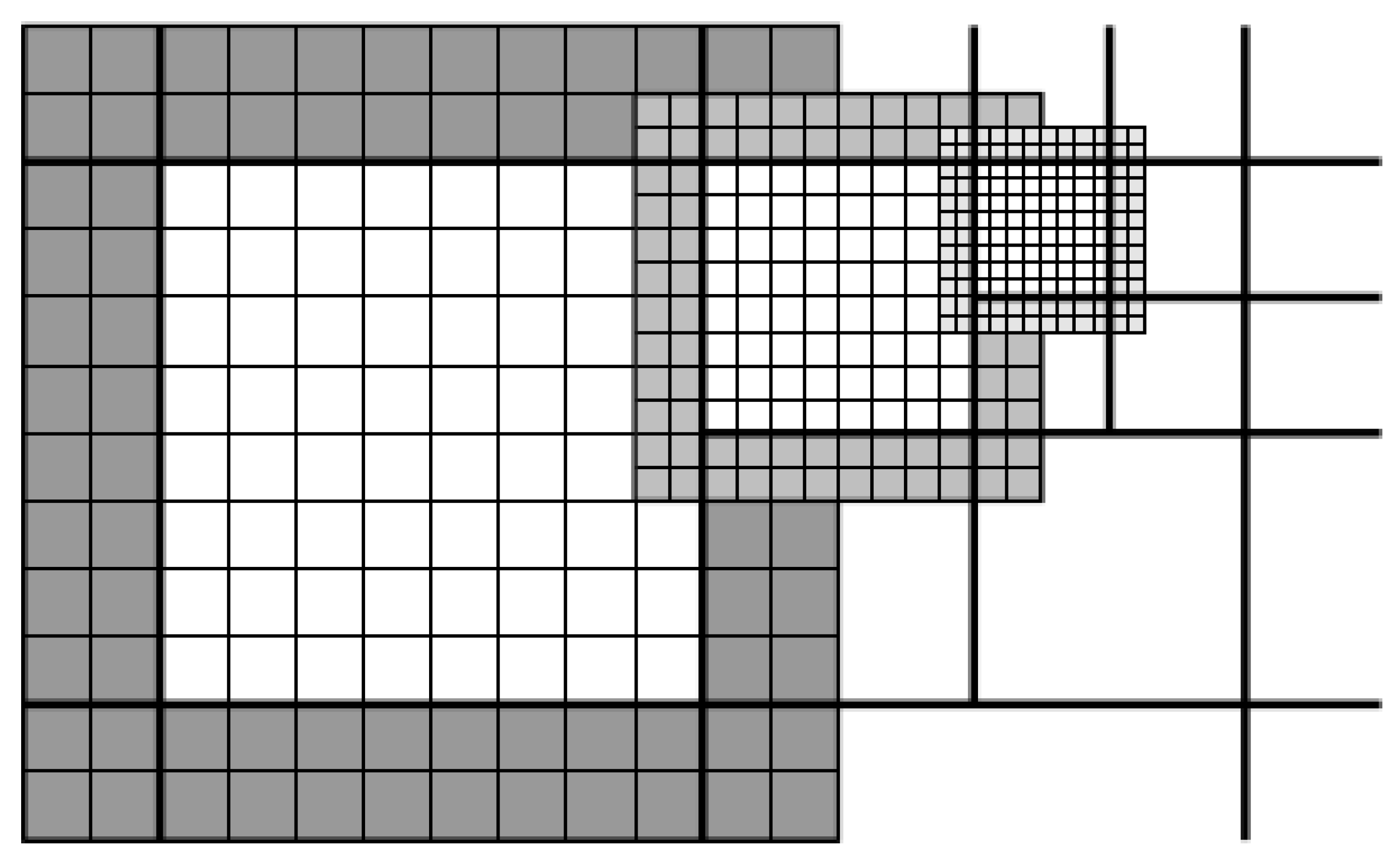
From the figure above, three levels of refinement are shown, a ForestClaw domain consists of a static arrangement of one or more blocks where by each is subdivided into more quadrants. During refinement, a quadrant will be partitioned in to four quadrants of the same size (level 1), further more the quadrants will be partitioned into four other quadrants and so on until when the resolution needed is achieved.
All the aforementioned software packages (P4est and Forest Claw) are integrated into GeoFlood with the objective of solving shallow water equations and GeoClaw is used to benchmark to eval- uate the performance of GeoFlood.This integration is motivated by their capability to accurately represent the behavior of water across a broad spectrum of flow conditions.
4. Methodology
The GeoFlood code integrates with libraries such as ForestClaw and P4est, supported by essential dependencies including Libtool, make, CMake, GCC 12, Git, MPICH-GCC 12 (version 12.0), zlib, and pkg-config.Libtool simplifies the creation and utilization of shared libraries, facilitating portability and maintainability (Matzigkeit et al., 1996).Make automates compilation, dependency management, and supports incremental builds, crucial for managing dependencies and installing packages like ForestClaw. CMake ensures code build and installation independence from user environments, vital for distributing the code effectively (Marson and Jankowski, 2016).GCC 12 is a compiler that compiles a source code into executable programs or libraries, while MPICH- GCC12 supports parallel programming with MPI.The zlib library enables data compression and decompression, optimizing storage requirements and resource utilization.Pkg-config is employed during compilation to ensure compatibility with the C compiler and library.
The topography data is collected from platforms like Google Maps and Google Earth, alongside various other sources.Topography is represented as digital elevation models (DEM) which can be categorized into three main types:
Type 1: This is a topography file consisting of three columns, namely x, y and z, where x and y represent positions of the physical features and z represents the elevation or depth.
Type 2: This is a topography file consisting of six headers, namely, number of columns(ncols), number of rows(nrows), xl corner, yl corner, cell size (dx or dy) and region with no data.
Type 3: This topography includes all six headers from Type 2 and includes topography lines with dimensions of mx by my, where mx indicates number of rows and my indicates number of columns.
The topography utilized in the Malpasset Dam benchmark that we will study was obtained from a bench marking exercise conducted in 1999 under the support of the CADAM (Concerted Action on Dam-break Modelling) project, a collaborative European research initiative.This bench marking effort, documented by (Frazao et al., 1999), involved a collection of 13541 points with irregular spacing and known coordinates, serving as the basis for defining the numerical domain.The Dam break referred to in this case is Malpasset Dam Break which will be talked about more in the next chapter.The topography for this incident is of 6 different forms, namely; domain-grid, reservoir, grid-4, grid-3, grid-2 and dam approach.In the process of addressing the issue of computational cost and improving efficiency, we need to efficiently handle topography in GeoFlood, a topic we will delve into shortly as we progress through this chapter.
The following figures show plots of the different topography/bathymetry files:
Figure 4.
1: Figure shows different bathymetry files.
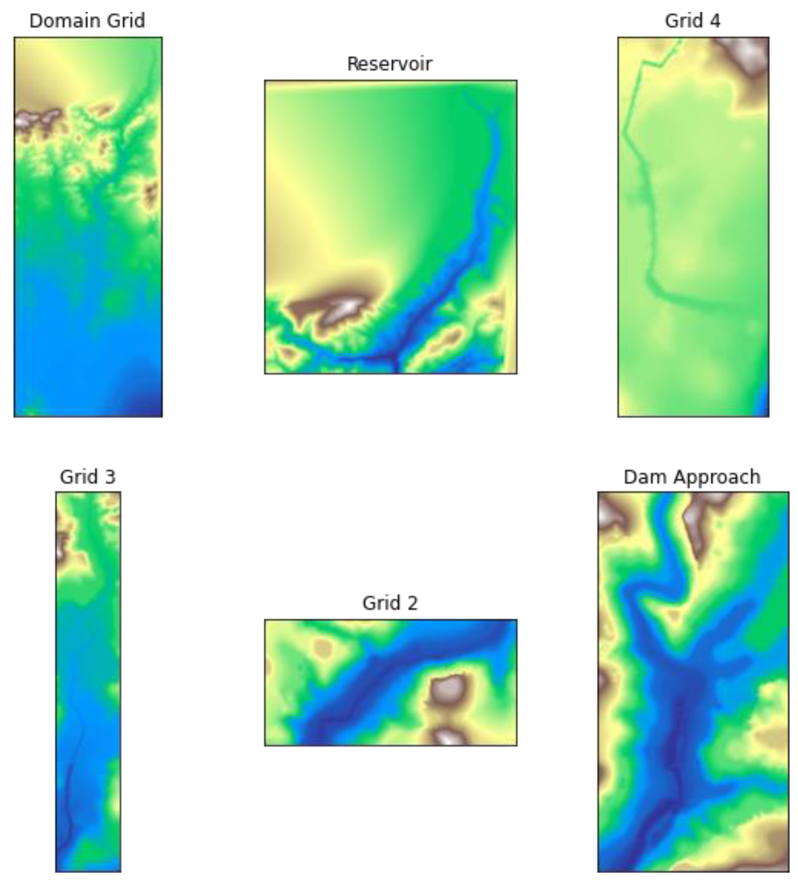
From the above, Domain grid represents the entire domain (spatial domain), Reservoir represents the location of the dam, Dam approach shows the area close to the dam and the other files (Grid 2, Grid 3 and Grid 4) show the path.
Figure 4.
2: the first figure shows the six bathymetry files plotted on the same plot, the second figure shows bathymetry files not yet discritized then the last figure shows files that are discretized.
Figure 4.
2: the first figure shows the six bathymetry files plotted on the same plot, the second figure shows bathymetry files not yet discritized then the last figure shows files that are discretized.
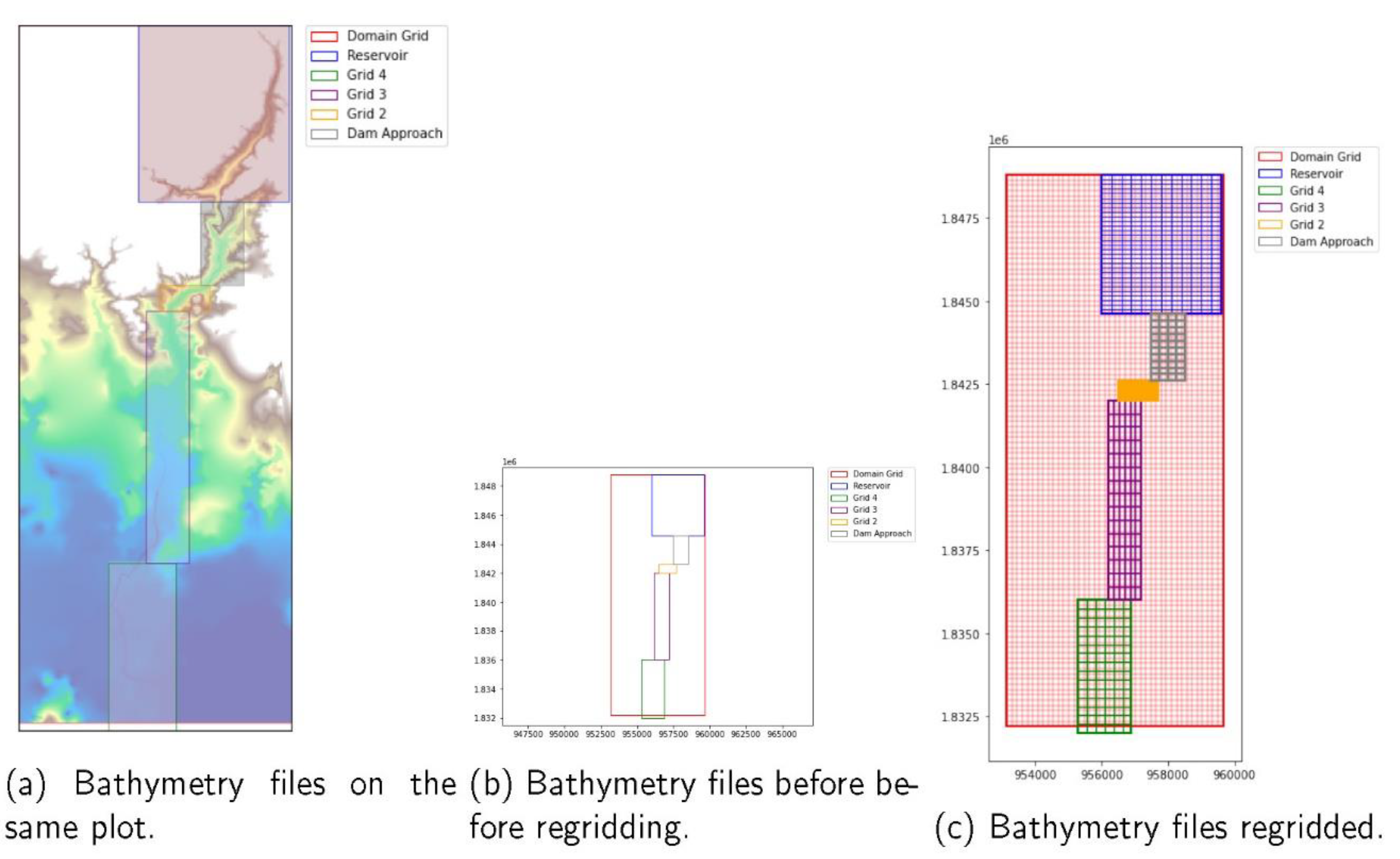
GeoFlood reads the topography/bathymetry files as rectangles punched or fit in one file (Domain file) as seen in figure (a) bellow.
When the files are combined into one, the rectangles will intersect and cells will overlap, as demonstrated in figure (c) (Reservoir intersects with Dam approach and cells for Domain overlap cells for Reservoir), posing a challenge during regridding.All of these concerns are addressed when handling bathymetry/topography in GeoFlood, as we will soon discuss.Regridding/refinement involves the computation of bilinear integrals.Bilinear integration involves dividing a given domain into different cells or portions, determining the area of each independent portion (in our case, for a single cell with four corners), and then integrating over the four corners to calculate the area of the entire domain.It is crucial to compute these bilinear integrals at the beginning and store them to prevent time-consuming recalculation during regridding.The application to be developed aims to provide these bilinear integrals so that they can be readily accessed whenever needed.
4.1. How Topography/Bathymetry Is Handled in GeoFlood
As its aimed at improving the efficiency of GeoFlood and addressing computational cost of GeoFlood during simulations of overland flooding, there are different scenarios that happen with
in topography data and may lead to inaccurate results like the overlapping of topofiles with different resolutions and yet our focus is more on those with highest resolution (finest topofiles) for accurate results, so such scenarios have to be catered for.
To show how bathymetry is handled by putting in to consideration the above scenario, we shall consider the following problem;
Problem: Let D be a union of overlapping rectangles Ri (topofiles)

The rectangles are ordered by resolution, so that the resolution of Ri is higher than the resolution for Ri+1 and so on.Over each rectangle/topofile, define a function Ti(ξ, η).Define a unique surface (grid cell/integration region) T (ξ, η), where
 where I is the smallest index for which (ξ, η) ∈ RI.
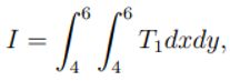
The problem is given a rectangular region C ⊂ R, compute the integral
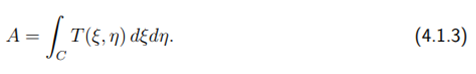
The above problem is to find the integral of the unique surface/grid cell over the overlapping rectangles/topofiles, and to achieve this, we are going to solve it or show how it is handled using a case scenario of a few topofiles with defined functions, we shall see what happens when the grid cell is embedded with in the finest topofile and when it intersects the other topofiles.
Below is mathematically how we get the intersection of two topofiles (rectangles)
Mathematically how the intersection is computed
Let topofile-1 (T1) be defined by the vertices (x1, y1), (x2, y1), (x2, y2), and (x1, y2).Similarly, let topofile-2 (T2) be defined by the vertices (x3, y3), (x4, y3), (x4, y4), and (x3, y4).The inter- section region between the above 2 topofiles I is given as:
where
I = [xmin, xmax] × [ymin, ymax],
- xmin = max(x1, x3),
- xmax = min(x2, x4),
- ymin = max(y1, y3),
- ymax = min(y2, y4).
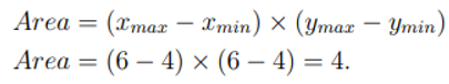
And area of the intersection region is given by
Area = (xmax − xmin) × (ymax − ymin).
So in regards to the above problem, below is the solution to the case study of three topofiles, now in this case the union of overlapping rectangles Ri contains Topofile-1 (red), Topofile-2 (green) and Topofile-3 (blue) arranged in a list from the finest to the coarsest.
Example 1:When the grid cell is embedded with in the finest topofile.
Figure 4.
3: Figure shows grid cell embedded in to the finest topofile.
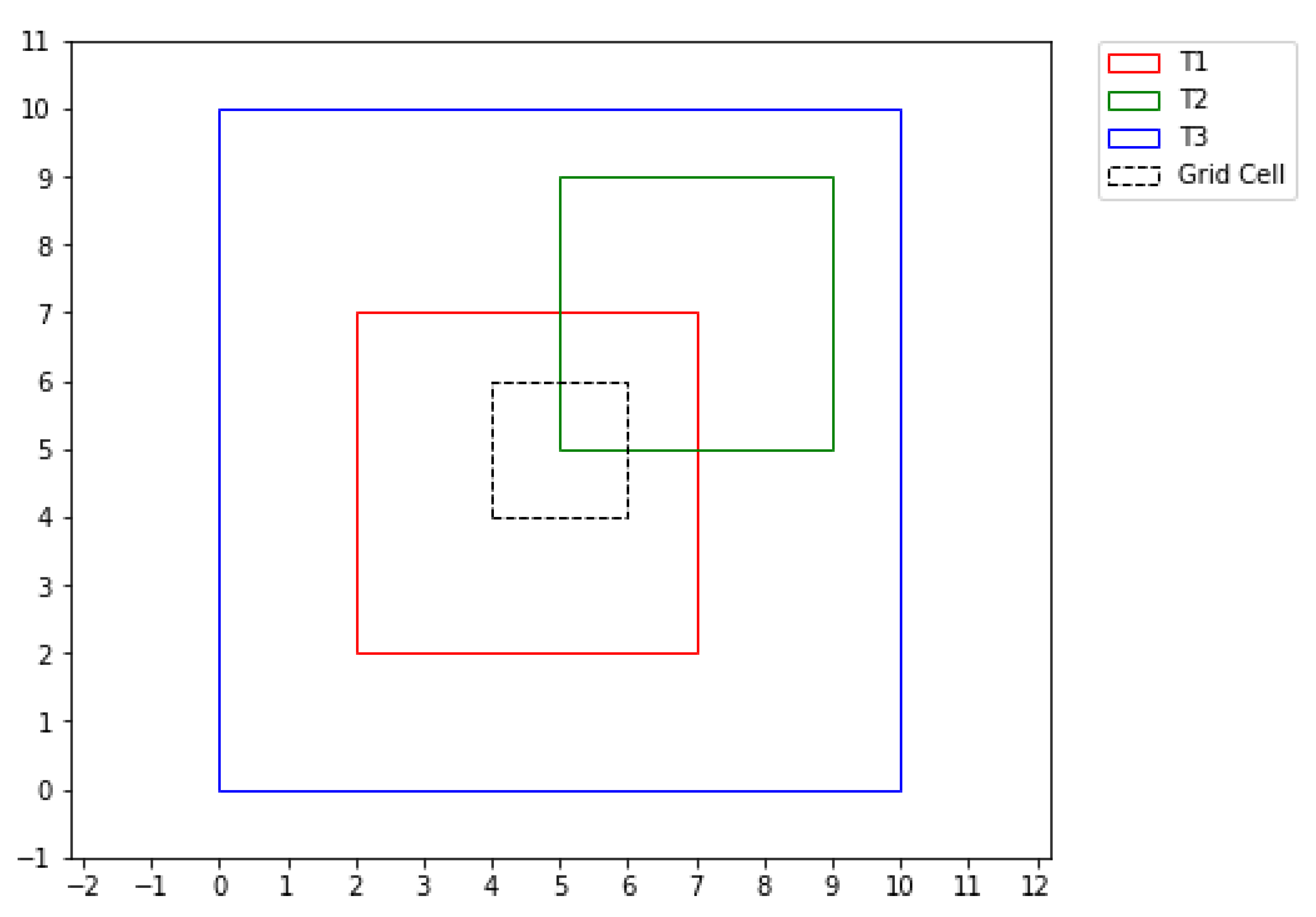
From the above plot, we have 3 rectangular topofiles with the following dimensions:.
Topofile-1(red) = [2, 2] × [7, 7],
Topofile-2(green) = [5, 5] × [9, 9],
Topofile-3(blue) = [0, 0] × [10, 10].
Let us assume the following:
- the grid cell be the black dotted rectangle with dimensions,[4,4] to [6,6],
- Topofile-1 be the finest topofile,
- Topofile-2 be the medium (fine and coarse),
- Topofile-3 be the coarsest topofile.
Recall that we are interested in accurate solution, so we are always interested in the topofile with the highest reolution (finest topofile) so the grid cell whose integral we are interested in always come from the finest topofile, so from the figure above, it clearly show that the grid cell is embedded with in the finest topofile but still this can be seen mathematically as shown bellow.
First step:We compute the area of the grid cell:
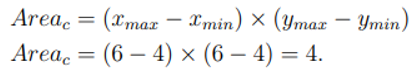
Second step:We find the intersection region between the finest topofile and the grid cell, then compute its area.The intersection region is [4, 6, 4, 6] and the area of the intersection region is
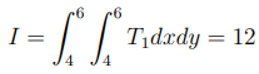
Third step:Check if the Area of the grid cell is the same as that of the intersection, now for this example its the same, meaning the grid cell is embedded with in the finest topofile and since we are interested in the finest one, we just compute the area of the grid cell or the integral of the grid cell using the function of the finest topofile.
where f1 is a function assigned to topofile-1 (finest topofile), similarly other topofiles are assigned functions like T2 for topofile-2 and T3 for topofile-3.
If given T1 = 3, then we have
Lets now see another example where the grid cell is not entirely embedded with in the finest topofile, but rather intersects with other topofiles.
Example 2:
Figure 4.
4: Figure shows grid cell embedded in to the finest topofile.
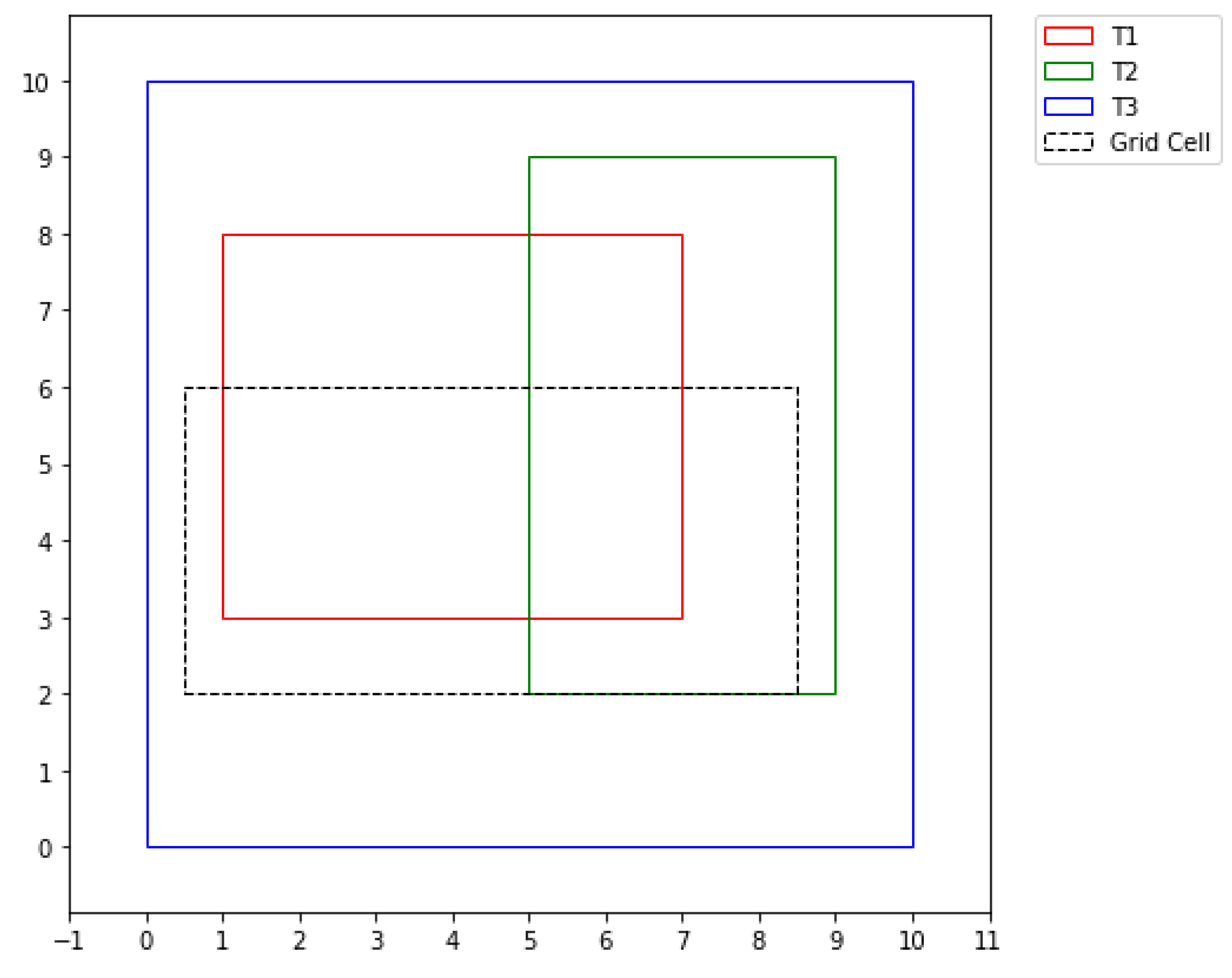
The above graph shows rectangles/topofiles with the following dimensions:
topofile-1(T1) = [1, 7, 3, 8],
topofile-2(T2 = [5, 9, 2, 9],
topofile-3(T3) = [0, 10, 10],
Grid cell = [0.5, 8.5, 2, 6].
Similarly the above topofiles are also arranged from the finest to the coarsest topofile,and associ- ated with functions, f1, f2 and f3 respectively.So to calculate the integral of the grid cell in such scenario, we shall have to compute the independent integrals for each intersection of the grid cell and the different topofiles, which is shown below.
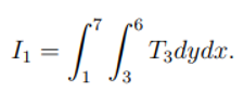
The intersection region of topofile-1 and the grid cell is[1, 7, 3, 6].
The integral (I1) of the region is
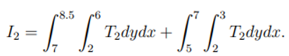
The intersection regions of topofile-2 and grid cell are [7, 8.5, 2, 6] and [5, 7, 2, 3].
The integral for these regions I2 is computed from
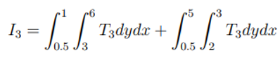
The intersection regions of topofile-3 and grid cell [0.5, 1, 3, 6] and [0.5, 5, 2, 3]
The integral (I3) for these regions is:
So to get the total integral (I) of the grid cell, we shall have to sum all the independent integrals computed above, that is;
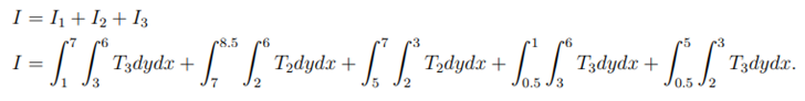
If given the values of the functions, say T1 = 3, T2 = 2 and T3 = 1, then the integral is

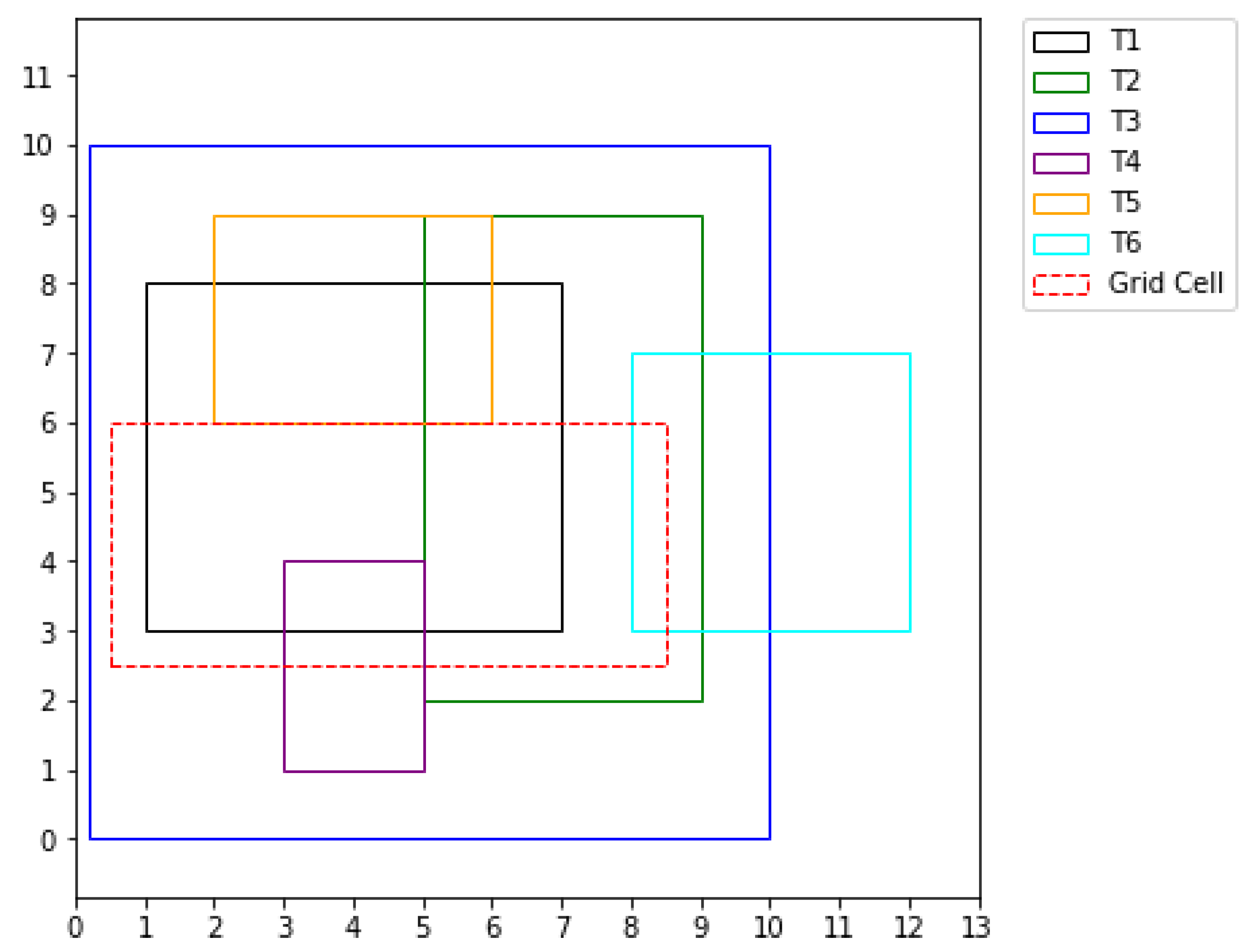
However we may have cases where the integral may not be computed easily or its time consuming, that is in cases when the topofiles are many or in cases when they are of large dimensions, for example the figure below. In such cases a subroutine was written to to compute these integrals and it can be referred to by the Pseudo code written down.
Example 3:
The figure above shows six topofiles and the grid cell (red), in the above figure it may take you time to compute the integral of the grid cell manually or even you may be in position to do so but end up getting a wrong answer, so in such cases, and due to the fact that in real life problems we deal with huge sums of data, a subroutine following the Pseudo code below was written.
Figure 4.
5: Figure shows grid cell overlapping more than three topofiles.
Algorithm to compute integral of a grid cell
4.1.1. Functions Assigned to Each Topofile and Topofiles Initialized
- Define topography functions assigned to each topofile for example T1, T2, T3) and so on.
- Define the dimensions of the grid cell, say a list with [xmin, xmax, ymin, ymax]
- Define a list of topofiles and their respective dimensions. (for the dimensions, you may need only the lower left coordinates and the upper right coordinates for each topofile).
4.1.2. Define a Function to Check for the Intersection of Two Topofiles
-
Function: intersection(r_1, r_2):
- -
- It will take in two rectangles
- -
- It will compute the intersection.
- -
- Check if there exists the intersection, if so it then computes the area of the intersection.
- -
- It will return the dimensions of the intersection region and the area if it exists, if it does not, it will return area as 0.
4.1.3. Define Function to Recursively Compute the Integral of the Grid Cell
This function helps to compute the integral incase the grid cell is not embedded with in the topofile with highest resolution but when its overlapping with so many other topofiles of different resolution.
-
Function: compute_integral(grid_cell, m):
- -
- It will take in the grid cell and index of the current topofile as arguments.
- -
-
Set the number of topofiles.
- *
-
Base case:
- It will check if the topofile is the coarsest (the last one in the list).
- If topofile is the coarsest, it will compute the area of the intersection between that topofile and the grid cell using the above intersection function, and also returns that area and the dimensions of the intersection region in case it exists.
- If the area is zero, that is no intersection, it returns zero (0).
- *
-
Recursive case:
- If the topofile is not the last one in the list (coarsest), it will make a recursive call to compute the integral (First integral) for the next topography file in the list.
- It will again calculate the area of the intersection between the grid cell and the current topography file.
- If the area is positive, that is,there is an intersection.
- It will define the intersection region as the intersecting sub-region of the grid cell.
- It will again make a recursive call to compute a second integral, over this intersecting region to be subtracted from the First integral to cater for over- laps.
- It will compute the Third integral as the area of intersection multiplied by the function value of the current topofile, to be added to the First integral to correct overlaps.
- Then finally it will return an integral as First integral-Second integral+Third integral.
4.1.4. Define the Main Function/Routine Which Will Then Call the First Two Functions to Compute the Integral
-
Function grid_cell_int(grid_cell):
- -
- It will first calculate the Area of the grid cell using its dimensions.
- -
-
It will then iterate through the topofiles.
- *
- For each topofile, it will check if there exists an intersection between each and the topofile by calling the intersection function above.
- *
- If the area of the intersection between the topofile and the grid cell exists and its equal to that of the grid cell, it will the compute the integral asI = Area × function assigned to that topofile
- *
- If its found that the area of the intersection is less than that of the grid cell, it will compute the integral recursively by calling the recursive function. This is because for this case there will be overlaps, so they have to be handled well to avoid double counting which may lead to over estimation or under estimation of the integral.
- *
- This is the function the returns the integral of the grid cell.
Note: Note that the above algorithm can still change. The functions can be defined in any way that is easiest, provided the overlaps are handled efficiently and accurately, and computational time is also taken into consideration.
4.2. How the Above Is Done in Real Case (Piecewise bilinear Surface)
A computational domain is created from a union of rectangular topofiles.Data in the topofiles is a collection of points on a Cartesian grid.The lower left and upper right corners of the topofile, along with the number of points and the cell size is specified in the file.For example, one of the topofiles in the Malpasset Dam problem has 20m resolution (e.g. cell size) and 953155 × 1832200 points.
The challenge is to define the function Ti(ξ, η) for a particular topofile

where (ξ, η) is in topofile cell tm,n.
Define a bilinear function of the form
where a,b,c and d constants for the rectangular region representing a mesh cell [ξ1, ξ2, η1, η2] in the topofile.These bilinear functions are computed and combined to form the overall surface.They are combined in such a way to allow continuity at the boundaries of each.
tmn(ξ, η) = aξ + bη + cξη + d
The value of the bathymetry over a computational mesh cell Cij is defined as the average value of this piecewise bilinear surface over the computational cell and is given by
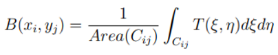
The mesh cell Cij is now the grid cell referred to in the previous examples.
Lets look at the integral of the bilinear function of a rectangular surface mathematically.
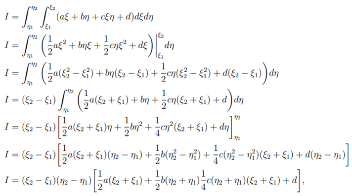
where
Area(of the rectangular surface) = (ξ2 − ξ1)(η2 − η1).
Diagram showing an integral intersection with bilinear cells:
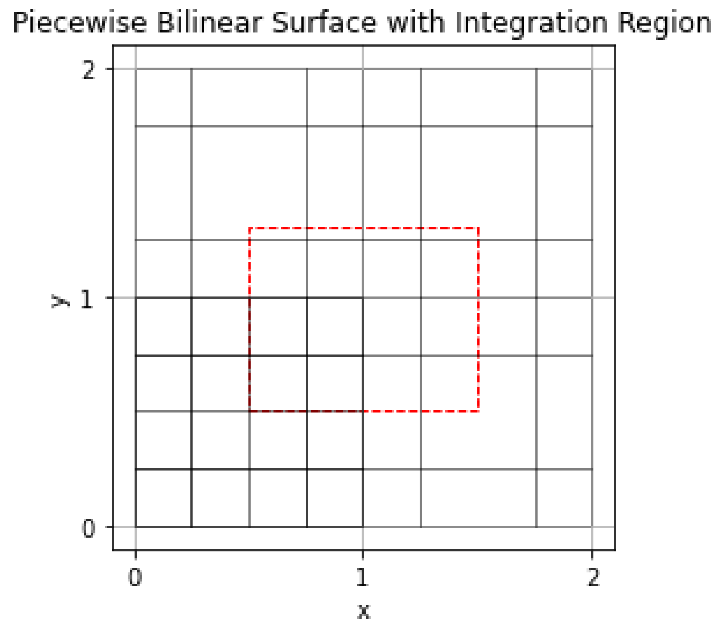
Figure 4.6 shows a piecewise bilinear surface in 2D with dimensions [0,2,0,2], bilinear cells (the black rectangles) with dimensions [0,1,1,2], [1,2,1,2], [0,1,0,1] and [1,2,0,1], with an integration region (red) with dimensions [(0.5, 0.5), (1.5, 0.5), (1.5, 1.3), (0.5, 1.3)] that intersects the multiple bilinear cells.
Figure 4.
6: Figure shows an integral intersecting bilinear cells.
5. Results and Discussions
5.1. Results
The Malpasset Dam, located about 12 km upstream from Frejus, France, was a slender arch dam built in a narrow gorge above the Reyran River valley to create a reservoir holding 55106 cubic meters of water.Unexpectedly, on December 2nd, 1959 at 21:14 hours, the dam catastrophically failed, generating a sudden acoustic shock wave felt in Frejus, indicating an almost instantaneous collapse.Standing at a height of 66.5 meters with a crest span of 223 meters, the dam’s arch was the only remaining structure after the failure, accompanied by significant erosion of the nearby rock bank.Investigations suggest that the arch dislodged from its base, triggering a rapid and sequential collapse (Valiani et al., 2002)
The incident resulted in 433 fatalities and significant infrastructure damages, including the oblit- eration of a 1.km section of free way and an adjoining bridge, and extensive flooding of Frejus.The downstream displacement of massive blocks indicated the power of the flood.The flood waves rose to approximately 20m above the original riverbed.For comprehensive understanding of the incident, you can refer to (Boudou et al., 2017).
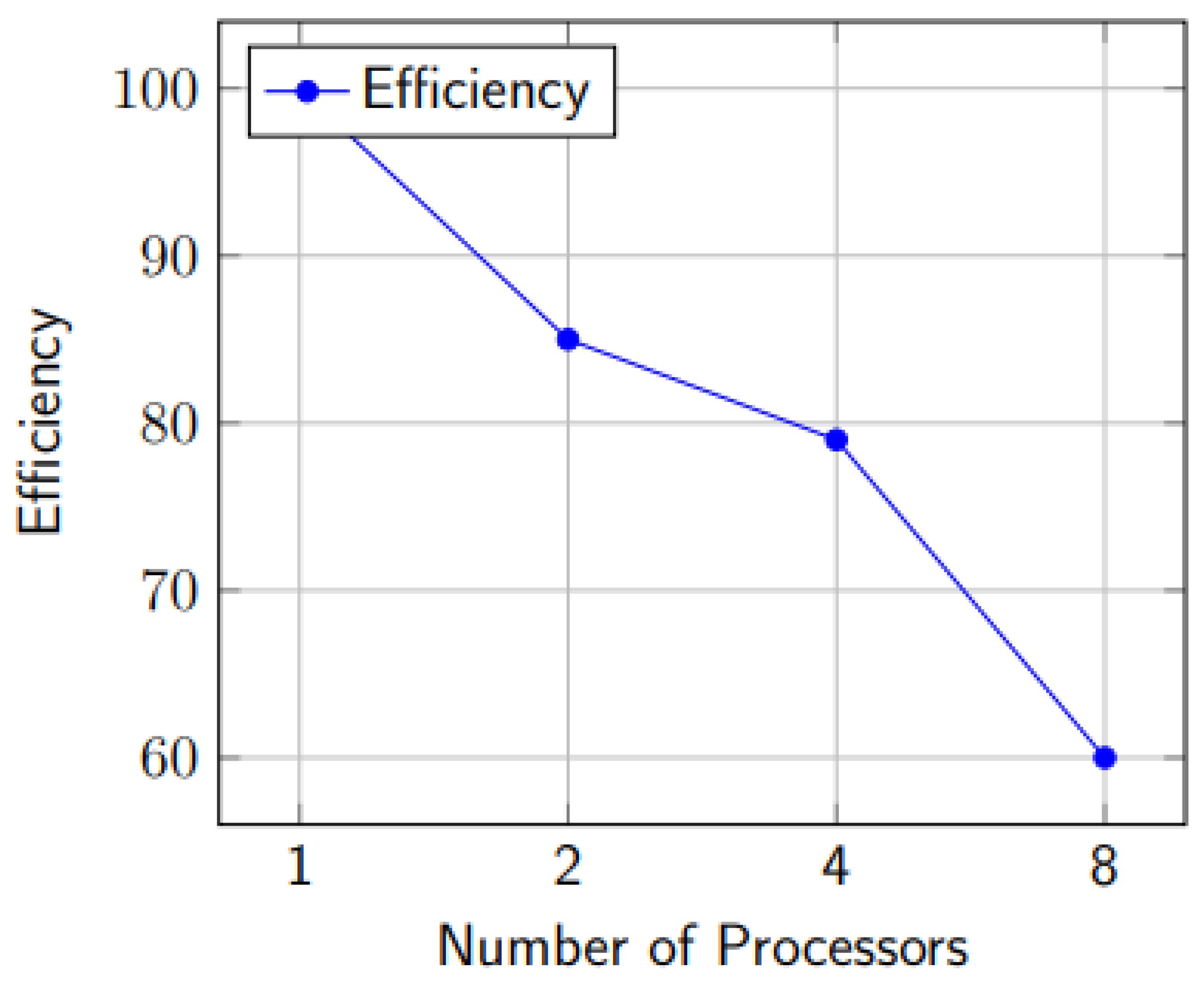
Before doing modifications with in the code, we ran the Malpasset data on different number of processors and below was the out come.Different processors were evaluated in terms of time taken when refining these data files and the wall time, advance time, Regrid time and Regrid-build times were recorded.This study aimed to assess the efficiency of various processors to identify opportunities for improving computational cost.Processors 1, 2, 4, and 8 were tested, and below are the achieved results.
Based on the results presented in the Table 1, the wall time for 8 processors was lower com- pared to that for 1, 2, and 4 processors. Similarly,the advance time was also lower compared to the other three cases.However, the Regrid time was higher than the other three cases, while the Regrid-build time was lower.For the case of 4 processors,the Regrid-build time was slightly higher than that for 2 processors.These results highlight that significant time is consumed during refine- ments, particularly evident in the Regrid time, despite the overall small wall time.It suggests that increasing the number of processors leads to a reduction in wall time, but further enhancements are necessary during refinements to optimize computational costs.
Figure 5.1 shows efficiency against number of processors used to run on the Malpasset data and it is found out that really the efficiency on 8 processors is not very bad (60%) but still it needs to be improved to raise the percentage, this is because the more the number of processors, the tasks are distributed equally to the processors which means time taken to do the regridding will be shortened.
Figure 5.
1: Efficiency (On Wall time) against Number of Processors.
Note that the aforementioned results were obtained under the following conditions: the final time was set to 600.0 units, the number of equations (shallow water equations) solved was 3, the topography domain spanned [953236.0, 959554.0] × [1832407.25,1848572.75],the number of refinement levels was 4, ranging from level 1 to level 4, and the grid dimensions were [16,16].
At present, every time regridding or refining occurs, processors must recalculate integrals, which, as observed in the above results, is time-consuming.This implies that the more levels of refinement there are, the longer the time taken.However, in many cases, we require finer refinements, which necessitate more integrals.Therefore, we must address this issue.
Bellow are some of the pictures showing the incident of the Malpasset dam break.
Figure 5.
2: Figures show Malpasset dam break incident at different time intervals.
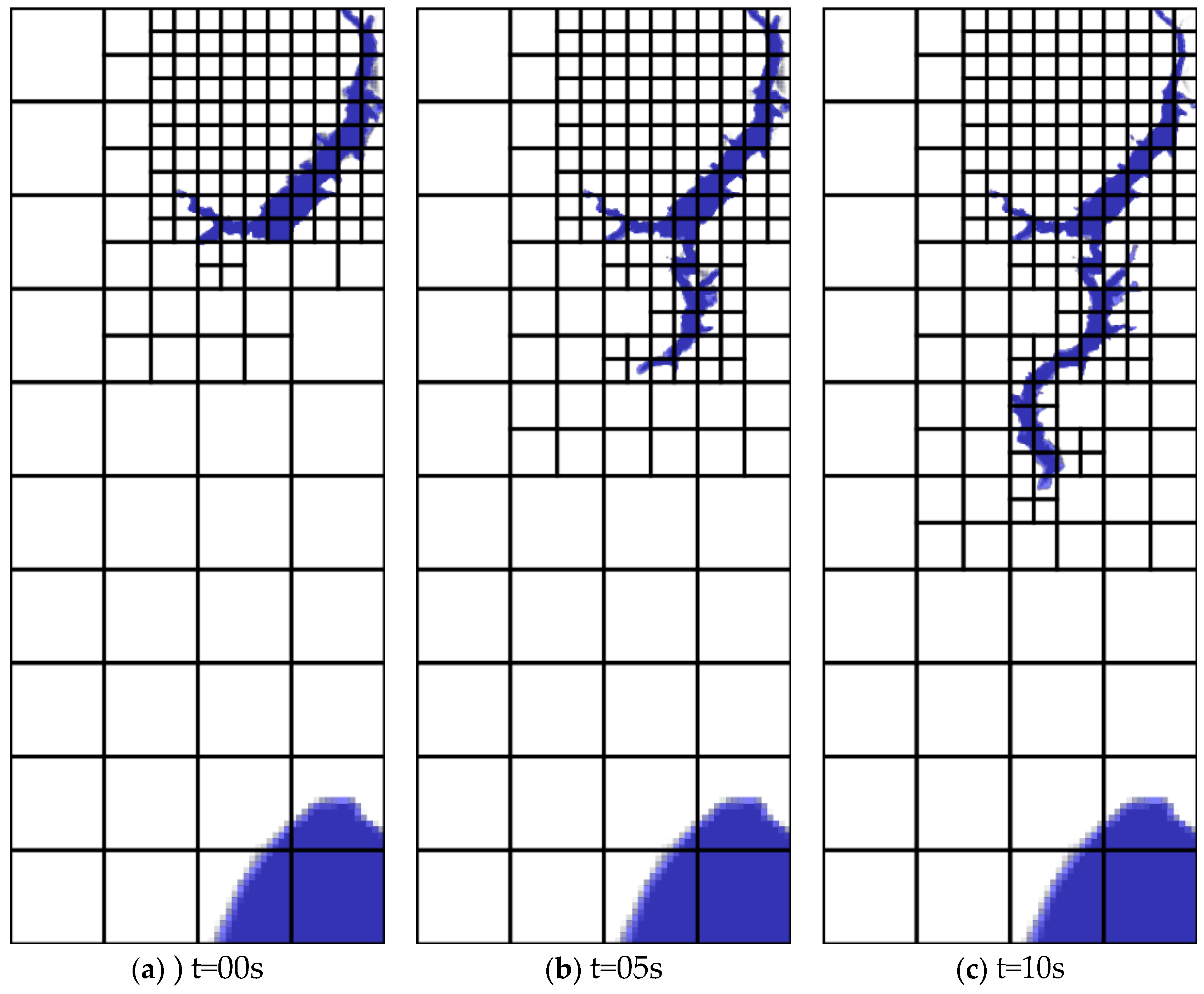
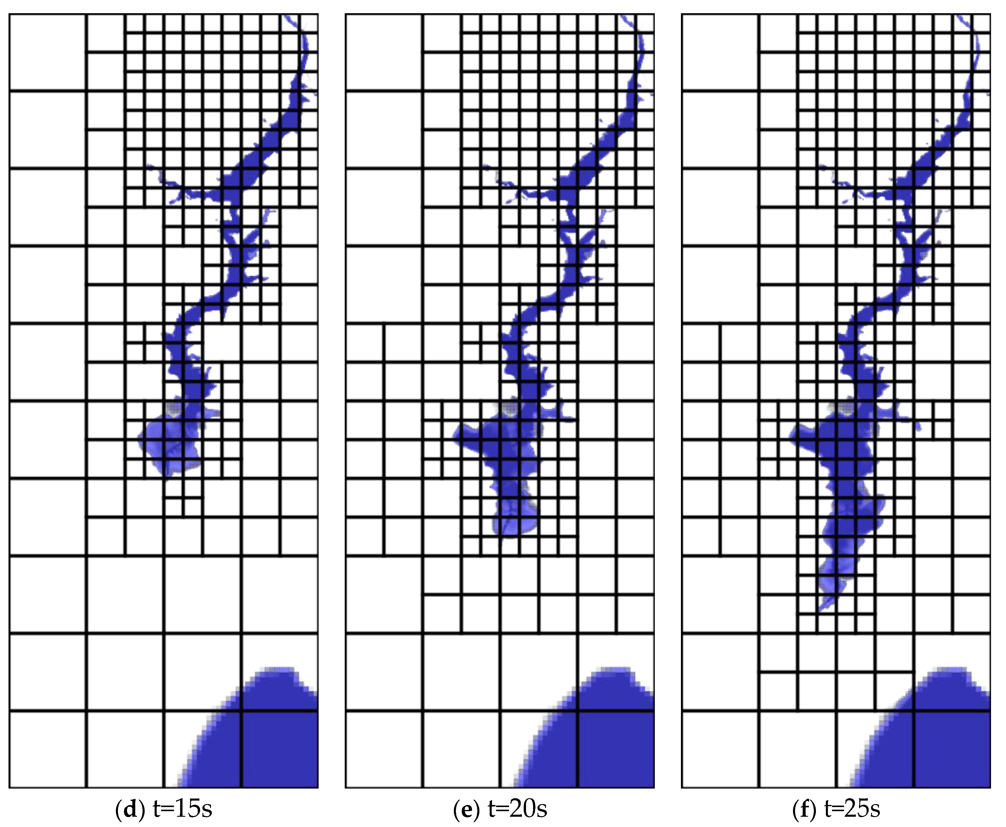
Figure 5.
3: Figures show Malpasset dam break incident at different time intervals.
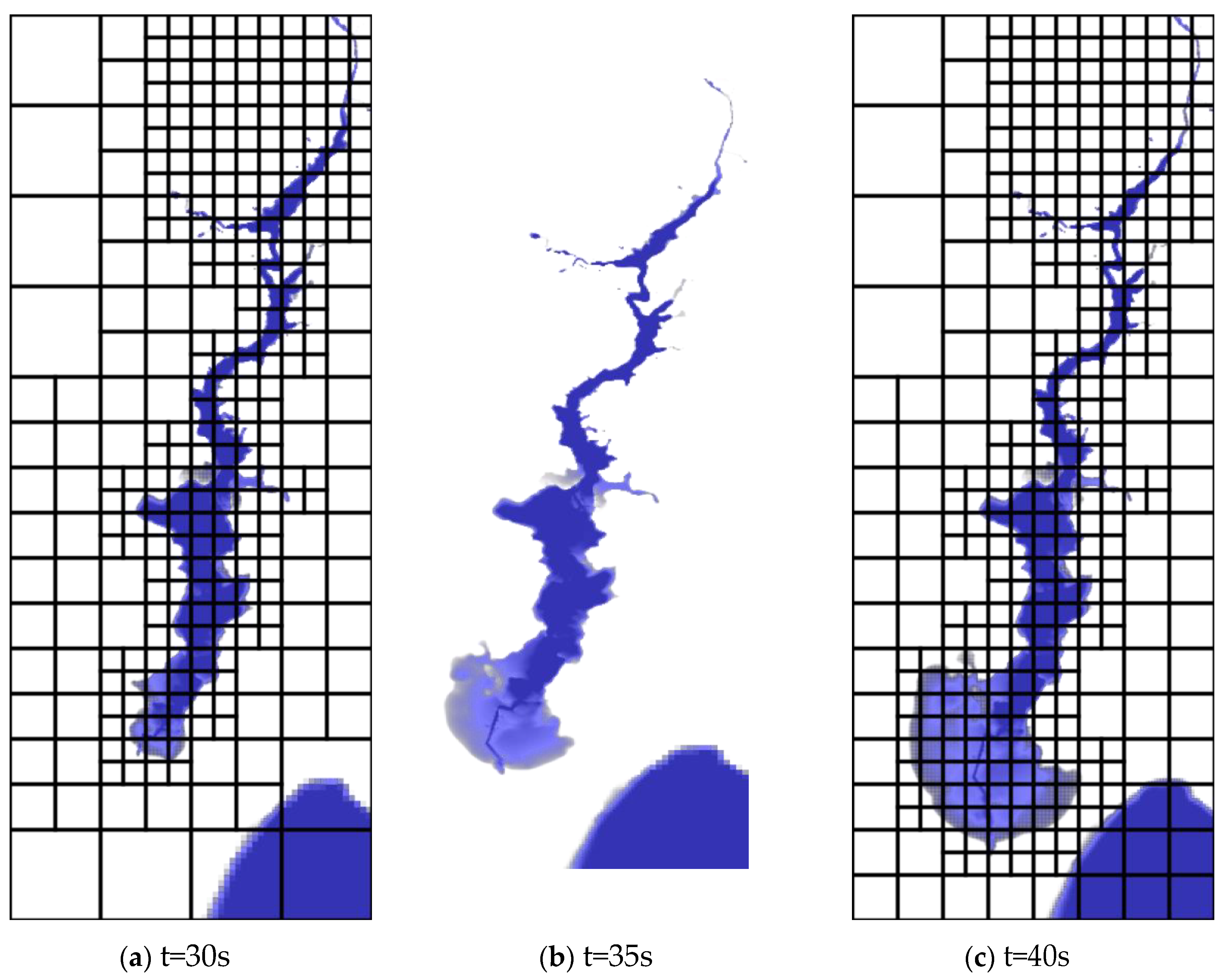
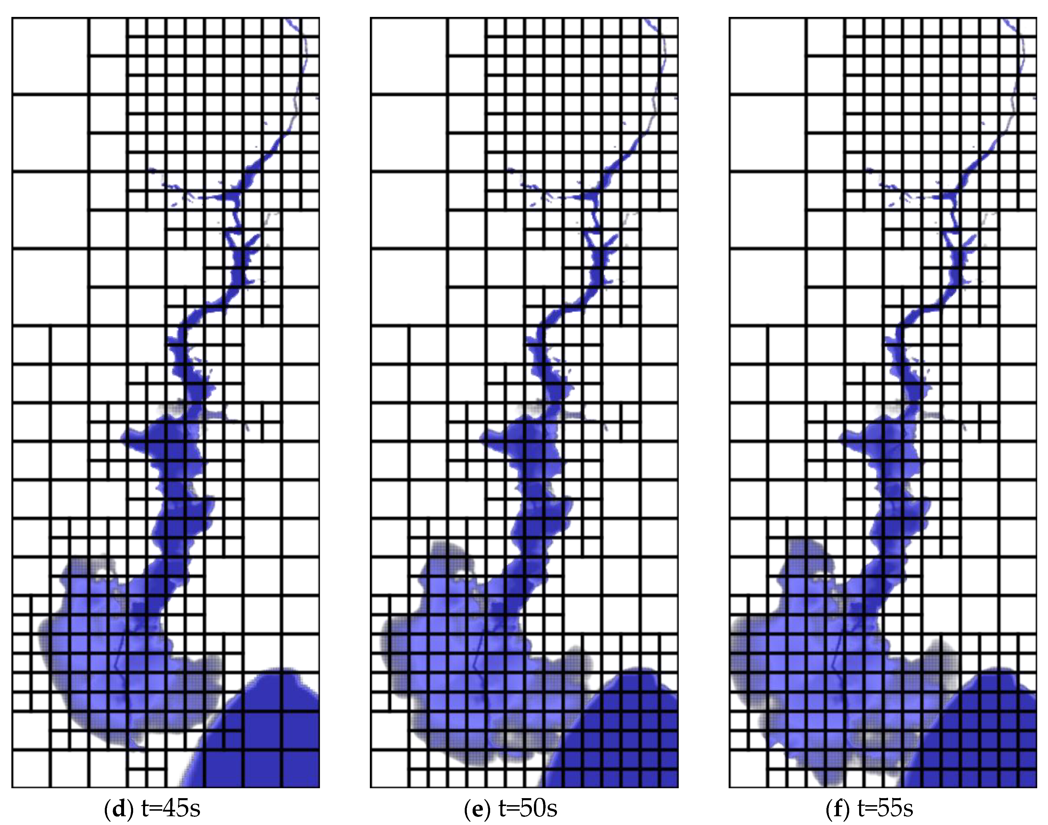
The above sequence of figures, show the incident of the Malpasset dam break at different time intervals.They were illustrated using google earth imagery.
5.2. Discussions
From the figures above, at time t=0s, the event shows a full reservoir with the dam intact. But as time went on, that is to say at 5s, 10s, 15s etc, the dam failed, which led to flood waters over topping the A8 highway. Between time t=15s, and t=25s, the flood waters proceeded through the valley, reaching Frejus.At time t=55s, the flood waters had reached the sea, hence the progression of the incident.
The Figures 5.2 and 5.3, they as well show refinements performed, adaptive mesh refinement applied in the simulation at time intervals of t=0, 5, 10 up to 55 seconds.At the initial time t=0s, the reservoir area was refined up to level 3.As time moved on, the broader region affected by the floods was refined at varying levels from l=1 to l=3, while the other parts not affected by floods were coarsely refined, that is to say were subjected to low resolution.
5.3. Initial Conditions and Boundary Conditions for Malpas- Set Dam Breakdown
Here the sea level and the initial reservoir level are assumed to be constant are set at 0 and 100m above sea level respectively.Although the outlet gate near the bottom of the dam was open during the incident, we neglected pre incident stream flow in the channel, that is to say the bottom of the dam was considered to be dry.Since the actual pre incident stream flow discharge is unknown, it was assumed to be negligible. Similarly since the value of the inlet discharge upstream of the reservoir is unknown, an imposed discharged constant of zero was used.The sea level was maintained constant (equal to zero).Note, we assume a short period dam failure.
5.4. Simulation Results for the Malpasset Dam Break before the Modifications Were Made
In the simulations before modifications in the code were made, we used a manning coefficient of 0.03333.The simulation runs were done on a 2.3 GHz i7 processor with 16 GB RAM.The simulations were performed on the computational grid or domain of dimensions 32 80 meters, with refinement levels from l=1 to l=3.The initial time step of 1 second, relying on a Courant- Friedrichs-Lewynumber (CFL) of 0.75.Note that CFL is a dimensionless number that ensures stability and accuracy during simulations, it is usually related to the ration of time step size to grid spacing.The adaptive mesh refinement criterias (flags) were designed basing on various conditions such as water depth, bathymetry, velocity, topographical features and the origin of the flood.This model accurately represented the flood’s domain and intricate details in the areas surrounding the flood plain during the dam failure as shown in figures 5.2 and 5.3.
The model led to the generation of simulations with high resolution mesh adaptations in the areas around the dam and flood plain as shown in the figures above.But still modifications are required to improve efficiency and reduce on the time taken during simulations.
5.5. GeoFlood Compared to Other Models to Simulate Max- Imum Water Elevations
To confirm that GeoFlood is the best fit to simulate overland flooding, it was compared with other models like GeoClaw, physical model data, static fitted mesh and Telemac2D to simulate the maximum height of the water.
From the Figures 5.4 and 5.5, the comparison drawn between GeoFlood simulated results at the 17 field-surveyed and 9 gauge locations against the field and experimental data (Frazao et al., 1999), with numerical results from GeoClaw, physical model data, static fitted mesh and Telemac2D.
Figure 5.
4: Police-surveyed points.
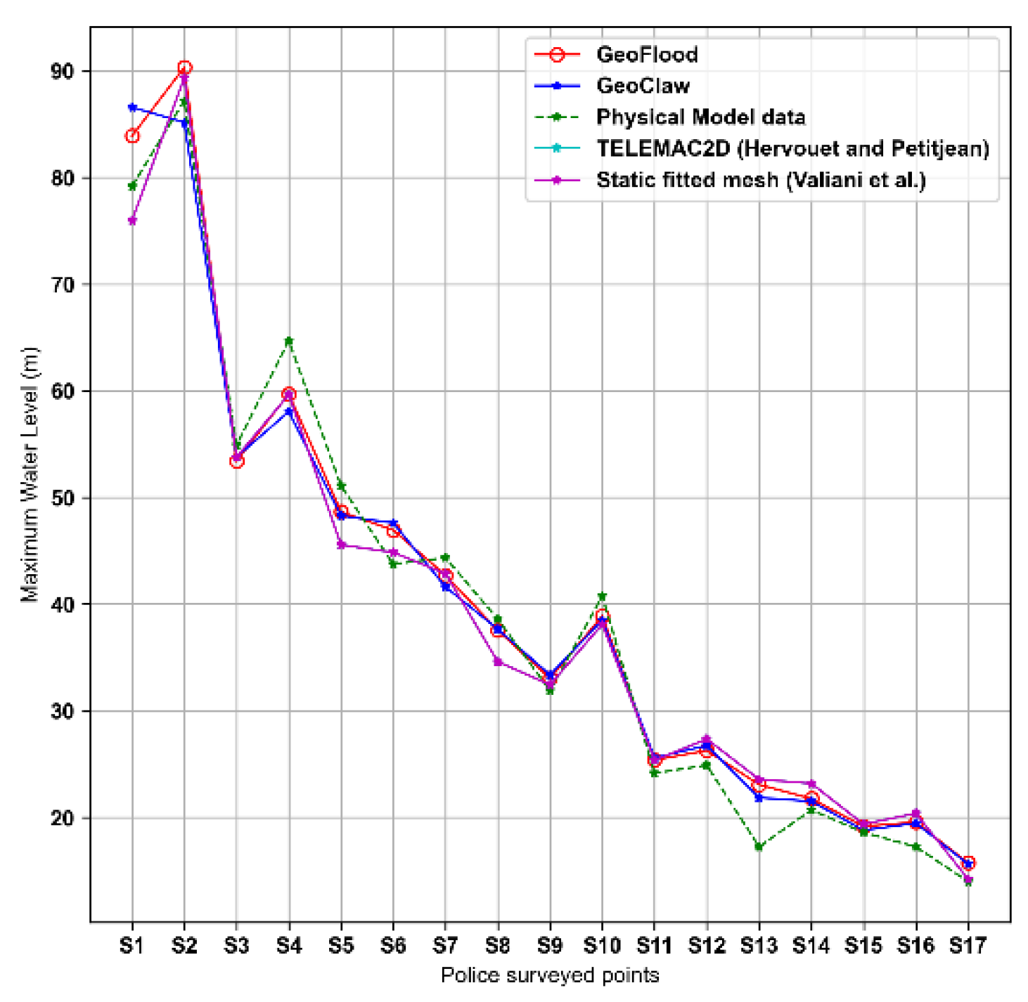
Figure 5.
5: Gauge points.
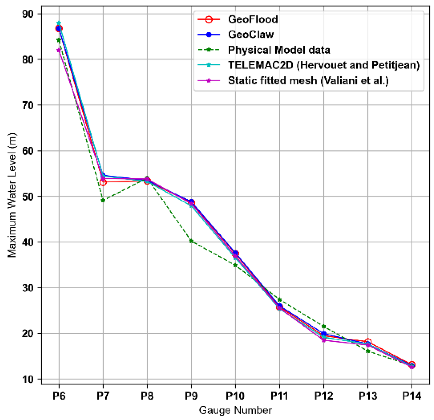
GeoFlood’s parallel grid management supported by Forest Claw allows the model to effectively monitor the flood’s extent and dynamically adjust the wet-dry boundaries during the refinement process. Field-surveyed locations tend to have a higher margin of error compared to gauge points. We attribute this to the fact that they are located near the margins of the flow. Given that all the models in comparison are based on shallow water equations,the prediction capability of different codes is most clearly differentiated by their ability to track the flood extents at the field-surveyed locations(Kyanjo et al., 2024). And it is evident that GeoFlood simulates well the maximum of water elevations.
6. Conclusion and Future Work
6.1. Conclusion
During this research I was able to install GeoFlood and configurations were made, GeoFlood was ran on a Malpasset data (for the dam failure) using different number of processors but it was found out that the efficiency needs to be improved and also the computation cost needs to be addressed.These issues are supposed to be addressed by finding an approach that efficiently handles bathymetry data.I also understood how bathymetry is handled with in GeoFlood during simulations.
6.2. Future Work
The main goal to address the above issues is to integrate adaptive mesh refinement (AMR) topography techniques into GeoFlood topography routines, leveraging the p4est (parallel mesh management library) routines to optimize topography handling(Burstedde et al., 2011).Then use new coupling techniques available in GeoFlood through p4est to provide topography on a distributed quad tree mesh.This technique is expected to be more efficient for real-world problems with complex and large domains.Then validate new developments against already existing test cases (Malpasset dam failure) and compare the results.So all the above was not able to be reached due to time hence calls for future work to be done so that the new features of P4est are coupled with in GeoFlood in order to enhance the efficiency and also reduce the computational cost during simulations.
Acknowledgments
I would like to express my appreciation to all those who have contributed to the completion of this research, both emotionally and academically. First and foremost, let me take this opportunity to thank my supervisor Prof. Donna Calhoun and co-supervisor Mr. Kyanjo Brian for giving me this opportunity to work with them on this interesting project, I thank all of them for the time and assistance I needed throughout the two months of my essay phase. I would like to as well thank all the tutors, but a big thanks to Dr. Roger Ranomenjanahary for always guiding me during this period. I thank AIMS administration and IT department for the resources (like internet, computer) they have provided to me so that my research is carried on smoothly and also for the opportunity to improve my research skills. Finally, my heartfelt thanks go to my friends, Jackila Elliot Bitakwate, Joel Muwanguzi, Derrick Chilenga and Daphine Miriam Namugosa for the extra support they have provided through the discussions to see that we grasp the concepts well.I also thank my family but my wife in particular Zahara Lutalo Namusoke for their encouragement words and prayers so that I complete this journey with success.
References
- Boudou, M. ; Moatty, A.; Lang, M. 1 - analysis of major flood events: Collapse of the malpasset dam, december 1959. In Freddy Vinet, editor, Floods, pages 3–19. Elsevier, 2017. ISBN 978-1-78548-268-7. [CrossRef]
- URL https://www.sciencedirect.com/science/article/pii/B9781785482687500018.
- Burstedde, C.; Wilcox, L.C.; Ghattas, O. p4est: Scalable algorithms for parallel adaptive mesh refinement on forests of octrees. In SIAM Journal on Scientific Computing; 2011; Volume 33, pp. 1103–1133. [Google Scholar]
- Donna Calhoun and Carsten Burstedde. Forestclaw: A parallel algorithm for patch-based adaptive mesh refinement on a forest of quadtrees. arXiv preprint 2017, arXiv:1703.03116.
- Clawpack Development Team. Clawpack software, 2024. URL http://www.clawpack.org. Version 5.10.0.
- Sandra Soares Frazao, Francisco Alcrudo, and Nicole Goutal. Dam-break test cases summary 4th cadam meeting. 1999. URL https://api.semanticscholar.org/CorpusID:109693772.
- George, D.L. Finite volume methods and adaptive refinement for tsunami propagation and inundation. University of Washington, 2006. [Google Scholar]
- George, D.L. Augmented riemann solvers for the shallow water equations over variable topog- raphy with steady states and inundation. Journal of Computational Physics, 2008; 227, 3089–3113. [Google Scholar]
- Kyanjo, B. GeoFlood wiki. https://github.com/KYANJO/GeoFlood/wiki, 2023.
- Kyanjo, B.; Calhoun, D.; George, D.L. Geoflood: Computational model for overland flooding. arXiv preprint arXiv:2403.15435, 2024.
- LeVeque, R.J.; George, D.L.; Berger, M.J. Tsunami modelling with adaptively refined finite volume methods. Acta Numerica, 2011; 20, 211–289. [Google Scholar]
- Mandli, K.T.; Ahmadia, A.J.; Berger, M.; Calhoun, D.; George, D.L.; Hadjimichael, Y.; Ketcheson, D.I.; Lemoine, G.I.; LeVeque, R.J. Clawpack: building an open source ecosystem for solving hyperbolic pdes. PeerJ Computer Science 2016, 2, e68. [Google Scholar] [CrossRef]
- Marson, R.L.; Jankowski, E. Build management with cmake. In Introduction to scientific and technical computing, pages 119–132. CRC Press, 2016.
- Matzigkeit, G.; Oliva, A.; Tanner, T.; Vaughan, G.V. Gnu libtool, 1996. Alessandro Valiani, Valerio Caleffi, and Andrea Zanni. Case study: Malpasset dam-break simulation using a two-dimensional finite volume method. Journal of Hydraulic Engineering 2002, 128, 460–472. [CrossRef]

Table 1.
Timing results for different processors.
| No. of processors | Wall time(s) | Advance time(s) | Regrid time(s) | Regrid-build time(s) |
| 1 | 10729.7 | 9563.86 | 20.5029 | 1.01052 |
| 2 | 6313.88 | 4919.63 | 14.8174 | 0.541249 |
| 4 | 3381.63 | 2517.43 | 12.0432 | 0.25904 |
| 8 | 2205.49 | 1561.47 | 13.4691 | 0.173513 |
Disclaimer/Publisher’s Note: The statements, opinions and data contained in all publications are solely those of the individual author(s) and contributor(s) and not of MDPI and/or the editor(s). MDPI and/or the editor(s) disclaim responsibility for any injury to people or property resulting from any ideas, methods, instructions or products referred to in the content. |
© 2024 by the authors. Licensee MDPI, Basel, Switzerland. This article is an open access article distributed under the terms and conditions of the Creative Commons Attribution (CC BY) license (http://creativecommons.org/licenses/by/4.0/).
Copyright: This open access article is published under a Creative Commons CC BY 4.0 license, which permit the free download, distribution, and reuse, provided that the author and preprint are cited in any reuse.


