Submitted:
05 June 2024
Posted:
06 June 2024
You are already at the latest version
Abstract
Recently, there appeared in this journal (Beh and Lombardo \textbf{2022}, {\it Symmetry}, 14, 1103) a paper that showed how to perform a correspondence analysis on a two-way contingency table where Bowker's statistic lies at the numerical heart of this analysis. Thus, we showed how this statistic can be used to visually identify departures from perfect symmetry. Interestingly, Bowker's statistic is a special case of the symmetry-version of the Cressie-Read family of divergence statistics. Therefore, this paper presents a new framework for visually assessing departures from perfect symmetry using a second-order Taylor series approximation of the Cressie-Read family of divergence statistics.
Keywords:
Bowker's chi-squared statistic
; correspondence analysis
; Cressie-Read family of divergence statistics
; singular value decomposition
1. Introduction
The correspondence analysis of a symmetric contingency table, has been a topic of research undertaken by, for example, Greenacre [22] and Beh and Lombardo [10]. Both approaches involve the partition of such that
where is the matrix that reflects the symmetric part of the table and reflects the skew-symmetric part. This partition was considered in various context by many including, but certainly not limited to, Bove [14], Section 3 Constantine and Gower [16] and Gower [25].
The methods of Greenacre [22] and Beh and Lombardo [11] approach the visualisation of the departure from perfect symmetry using correspondence analysis by partitioning the transformed contingency table into a skew matrix and a skew-symmetric matrix, as (1) does. While both correspondence analysis approaches have (1) as a common thread, they are quite different. Greenacre [22] uses Pearson’s chi-squared statistic, , that centres the elements of the contingency table with respect to the mean of the row and column marginal totals, yielding two low-dimensional displays; one depicting departures from perfect symmetry and the other depicting departures from skew-symmetry. On the other-hand, Beh and Lombardo [11] use Bowker’s chi-squared statistic, [15], producing a single low-dimensional display depicting departures from perfect symmetry.
While the difference between and is that the former assesses departures from complete independence while the latter assesses departures from perfect symmetry, both can be expressed as a special case of the Cressie-Read family of divergence statistics (Cressie and Read [17]) when viewed as a goodness-of-fit measure. For more on how correspondence analysis can be performed on a two-way contingency table using the Cressie-Read family of divergence statistics refer to Beh and Lombardo [11]. Their method includes, as special cases, the classical approach to correspondence analysis [6,8,21,28], log-ratio analysis (LRA) [23,24] and the Hellinger Distance Decomposition (HDD) method [18,19]. Rather than using Pearson’s statistic as the numerical foundation, LRA and HDD use the modified log-likelihood ratio statistic [29] and the Freeman-Tukey statistic [20], respectively.
This paper presents a family of symmetry divergent statistics based on the two recent works of Beh and Lombardo [10], Beh and Lombardo [11] by demonstrating how a correspondence analysis can be performed for assessing departures from perfect symmetry of . To do so, this paper is divided into five further sections. Section 2 gives an overview of the classic test of the departure from perfect symmetry for a two-way contingency table. It also describes how the Cressie-Read family of divergence statistics can be used for performing such a test. This family is dependent on the power parameter where changes in lead to special cases of the family. In this paper we focus on the second order approximation of this family which yields exactly Pearson’s chi-squared statistic (), the Freeman-Tukey statistic () and the modified likelihood ratio statistic (). Section 3 describes the core interest of this paper; the development of a correspondence analysis framework that can be applied to a two-way contingency table to visualise sources of departure from perfect symmetry when using the Cressie-Read family of divergence statistics. As part of this discussion, we also show that when , the method described by Beh and Lombardo [10] is a special case of this new framework. Two examples are given that demonstrate the various features of this new framework. Section 4 studies a artificial contingency table which exhibits perfect symmetry when a constant is added to a cell frequency. As C increases, the artificial table exhibits features consistent with increasing departures from perfect symmetry and so this example examines the features of this correspondence analysis framework as C and change. Our second example (Section 5) examines the data of Wiepkema [33] that is concerned with 12 pre- and post-courtship behaviours of a small European fish called a bitterling (Rhodeus amarus Bloch). Some final comments on the framework outlined here are made in Section 6.
2. Test of Perfect Symmetry and the Cressie-Read Family of Divergence Statistics
2.1. Notation
Suppose we have an contingency table, , where the th cell entry has a frequency of for and . Let the grand total of be n and let the matrix of relative frequencies be so that its th cell entry is where . Define the ith row marginal proportion by . Similarly, define the jth column marginal proportion as .
2.2. Testing Depatures from a Hypothesised
Testing whether there is evidence of a statistically significant association between the row and column variables of N can be made by considering any member of the Cressie-Read family of divergence statistics
for any , where is some value of under a well defined null hypothesis. When assessing departures from complete independence for so that (2) is a chi-squared random variable with degrees of freedom. However, Cressie and Read [17] also presented a second order approximation of (2) around that is very useful for the purposes of applying correspondence analysis to N. This approximation is
2.3. Testing Departures from Complete Independence
Of course, any reasonable choice of may be defined but we will confine ourselves to briefly discussing its definition under complete independence and perfect symmetry. For the case where one is interested in assessing departures from complete independence of the variables of N, (2) is expressed as
The subscript “A” has been added to the left-hand side to show that this family of statistics assesses departures from complete association. The general nature of (2), and (4), ensures that specific values of lead to well defined and well understood measures of association, all of which are chi-squared random variables. These include Pearson’s chi-squared statistic, the log-likelihood ratio statistic, and the Freeman-Tukey statistic which are , and , respectively. The modified chi-squared statistic, the modified log-likelihood ratio statistic and the Cressie-Read statistic are also special cases such that and , and , respectively.
Beh and Lombardo [11] showed that a correspondence analysis of N when assessing departures from independence can be undertaken by making use of the second order Taylor series approximation of (2) around
resulting in
This approximation may be obtained by substituting into (3). See also pp. 94 – 95 Cressie and Read [17] for a derivation of this approximation of (4). This family of statistics gives exactly the following commonly used chi-squared statistics: Pearson’s statistic , the Freeman-Tukey statistic and the modified log-likelihood ratio statistic . In the context of correspondence analysis, serves as numerical foundations of the traditional approach, is the foundations of the method described in Beh, Lombardo and Alberti [12] and Cuadras and Cuadras [18], while serves as the foundations of LRA, a variant of correspondence analysis described by Greenacre [23]. A fourth chi-squared statistic that is commonly used in the context of contingency table analysis, and was discussed from a correspondence analysis perspective by Beh and Lombardo [11] is when yielding , a second order approximation of the Cressie-Read statistic so that .
2.4. Testing for Departures from Perfect Symmetry
Sometimes it is the case that the two variables of N are, say, identical but measured over two different time periods. It may be that these same variables are collected between two different cohorts. In cases such as these, it is more typical to analyse the departures from perfect symmetry between the rows and columns of N. Therefore, when testing for departures from perfect symmetry, the null hypothesis is
for and for .
Assessing whether there exists any evidence of symmetry between the variables of N in the population, p. 427 Agresti [1] and p. 321 Anderson [4] showed that the most appropriate choice of is
Therefore, the Cressie-Read family of divergence statistics can be defined for testing departures from perfect symmetry so that (2) can be expressed as
and is a chi-squared random variable with degrees of freedom. The subscript “S” has been added to the left-hand side of (7) to show that this family of statistics assesses departures from perfect symmetry. This statistic has been the topic of interest by Tomizawa, Seo and Yamamoto [30], Ando, Hoshi, Ishii and 98izawa [5] and Altun and Saraçbaşi [2]. Our focus will be to examine the role of a second order approximation of for performing a correspondence analysis to visually detect departures from perfect symmetry. Therefore, it presents a more general framework to the correspondence analysis discussed by Greenacre [22] and Beh and Lombardo [11].
2.5. A Second Order Approximation
A second-order Taylor series approximation of (7) around
can be obtained by substituting (6) into (3). Doing so yields the family of asymptotically chi-squared random variables with degrees of freedom under the null hypothesis of perfect symmetry, (6),
or, alternatively but equivalently,
There are three special cases of this family of divergence statistics that we shall consider in our analysis of symmetry in a two-way contingency table. The first is when :
which is just Bowker’s chi-squared statistic [15]. Beh and Lombardo [10] used this statistic as the basis for performing correspondence analysis to assess departures from perfect symmetry in N.
Secondly, suppose that we consider the case where (8) is evaluated when . Then, we can show that
is the Freeman-Tukey statistic when assessing departures from perfect symmetry.
The third special case of (8) is when . For this value of , (8) does not exist. However, we can obtain the limiting value of (8) as . Doing so means that we can use the Box-Cox transformation so that
Therefore,
simplies to
and is the modified version of the log-likelihood ratio statistic when testing for perfect symmetry in . Note that eq. (8.2-11) Bishop, Fienberg and Holland [13], p. 489 Haberman [26] and eq. (1.3) Ireland, Ku and Kullback [27] gave the (unmodified) log-likelihood ratio statistic:
for assessing departures from perfect symmetry in a contingency table.
When there is perfect symmetry between the variables of N so that (5) holds, (9), (10) and (11) will be zero. When there exists a statistically significant departure from perfect symmetry, we can visually assess the statistical significance of this departure then using correspondence analysis. We shall now show how (8) can be used to perform a correspondence analysis on N when assessing these departures.
3. Correspondence Analysis & Perfect Symmetry
3.1. The Divergence Residual
To perform a correspondence analysis on under the null hypothesis of perfect symmetry we first define the matrix of divergence residuals, , where its th element is
Note that when (so that we are concerned with the diagonal elements of ) these residuals are zero for all . Three examples of the form that (12) takes is when and (approaching) 0. Respectively, these values of give the residuals
The first of these, , is the th Bowker residual described by eq. (7) Beh and Lombardo [10] so that n times its sum-of-squares produces Bowker’s statistic, (9).
The second and third residuals are akin to the Freeman-Tukey residual and modified log-likelihood ratio residual, respectively, described by Beh and Lombardo [11], but are used when assessing departures from perfect symmetry. Note that n times the sum of squares of these two residuals gives (10) and (11), respectively.
For , it is assumed that all cells of the contingency table have non-zero frequencies so that for and . This is to avoid any problems with calculating the natural logarithm of zero. In the event that a zero cell frequency is observed, a simple remedy is to replace it with a small value, say 0.01. Alternatively, one may use more objective methods to accommodate for a zero cell frequency. Other residuals can also be obtained using alternative values of .
3.2. Is the Matrix of Divergence Residuals Skew-Symmetric?
One of the benefits of using Bowker’s statistic as the numerical basis on which to perform correspondence analysis is that the resulting matrix of divergence residuals is skew-symmetric. That is, when , has the property that . Therefore, and for , . It also means that the singular values, and the left and right singular vectors, of can be calculated by applying an eigen-decomposition to or, equivalently, . Ward and Gray [32] and p. 113 Gower [25] discuss that for a skew-symmetric matrix, like , that if S is odd then there will always be a zero eigen-value and positive eigen-values. If S is even there will always be S eigen-values that exist in pairs [16].
When , is not a skew-symmetric matrix, since there will be at least one cell where , , unless there is perfect symmetry between the variables of .
3.3. Singular Value Decomposition and the Divergence Residual
When assessing departures from perfect symmetry in , the correspondence analysis approach of Beh and Lombardo [10] involves applying a singular value decomposition (SVD) to the matrix . Since Bowker’s statistic is a special case of (8), this suggests that a more general family of correspondence analysis techniques can be developed for visualising departures from perfect symmetry. Such a general family can be developed using the family of statistics generated from (8). Therefore, a new general family of correspondence analysis techniques can be obtained by applying a SVD to such that, for the th cell,
where
and M is the maximum number of dimensions required to depict all of the association that exists between the variables of the contingency table. When then if S is even and if S is odd. For other values of , . The quantities and are the ith and jth element, respectively, of the mth left and right singular vectors of the matrix of divergence residuals for a fixed . The mth largest singular value is so that .
The matrix form of (15) and (16) is
with
being the matrix form of (16). Here, is a identity matrix, is the matrix where the th element is , is the matrix where the th element is , and is the diagonal matrix of singular values with as it’s th element.
While the Cressie-Read family of divergence statistics can be expressed in terms of – see (13) and (14) – it can also be expressed in terms of its singular values. To show this, substituting (17) into (13) leads to
when is of full rank so that . Therefore, the total inertia of can be expressed as the sum-of-squares of the squared singular values so that
Expressing the total inertia in this manner is analogous to the total inertia of p. 22 Beh and Lombardo [11] when the Cressie-Read family of divergence statistics is used as the numerical basis of the correspondence analysis of a two-way contingency table.
3.4. The Principal Inertia Values
Beh and Lombardo [10] showed that when assessing departures from perfect symmetry when is a contingency table, , has two equal singular-values whose squared values are
and are the principal inertia values of the first two dimensions of the correspondence plot when analysing a two-way contingency table. Similarly, when symmetry is of concern for contingency table, the three principal inertia values are
For both sized , the sum of their squared singular values gives Bowker’s statistic.
When analysing the symmetry of a two-way table using the Cressie-Read family of divergence statistics we can consider values of . For example, when is of rank 2 then amending Appendix A of [10] for shows that there will be two unequal singular values whose squares are
Note that when these squared singular values simplify to (19).
When , then (19) and (20) are satisfied only when there exists perfect symmetry between the variables of (in which case all squared singular values will be zero). This is because when , is not a skew-symmetric matrix.
We now turn our attention to the construction of the M-dimensional correspondence plot by defining and describing the principal coordinates for each row and column of .
3.5. Principal Coordinates
When visually portraying the categories of N, define the metric matrix by
Then the matrix of row and column principal coordinates is
respectively. These provide a more general set of principal coordinates than those of eqs. (14) & (15) Beh and Lombardo [10] who were concerned only with the case when . Although, the principal coordinates of eqs. (14) & (15) Beh and Lombardo [10] can be obtained by simply substituting into (23) and (24).
Defining the row and column principal coordinates by (23) and (24), respectively, means that the row and column spaces have the same metric that is based on the aggregation of across the two variables, irrespective of the value of . Such an aggregation is done since (7) relies only on the cell proportions and .
Post-multiplying both sides of (23) by and simplifying gives us an alternative expression for the row principal coordinates
Similarly, it can be shown that the column principal coordinates can be expressed in terms of such that
As we have already shown, is not a skew-symmetric matrix unless . In the event that then, as shown by Beh and Lombardo [10],
where is an block-diagonal and orthogonal skew-symmetric matrix so that
See Section 5.1 Beh and Lombardo [10] for examples of when and 4.
3.6. On the Total Inertia and the Origin
The total inertia of the two-way contingency table can be expressed in terms of the matrices of row and column principal coordinated given by (23) and (24). To show this, suppose we consider the total inertia in terms of the row principal coordinates. Then,
Similarly, we can also show that the total inertia can be expressed in terms of the column principal coordinates so that
Therefore, if there is perfect symmetry between the rows and columns of our two-way contingency table then the total inertia will be zero. When this happens, the position of the row and column principal coordinates will be located at the origin. Therefore, the origin is interpreted as the point in the low-dimensional space where there is perfect symmetry between the row and column variables. The further a point is away from this origin then the more deviation it has from the null hypothesis of perfect symmetry. When assessing departures from complete independence assessing the contribution of a row and column point to the association structure can be undertaken using the closed-form equations that yield confidence regions for each point; see Beh [7] and Beh and Lombardo [9] when and Alzahrani, Beh and Stojanovski [3] for other values of . Such regions have not yet been developed for studying departures from perfect symmetry and so we shall leave this for future study.
4. Example 1: Artificial Data
4.1. The Data
To examine how the Cressie-Read family of divergence statistics can be used for the purposes of applying correspondence analysis to visually assess departures from perfect symmetry we consider the artificial data set given in Table 1. Beh and Lombardo [10] used this contingency table to highlight the features obtained when using Bowker’s statistic and so we shall focus on showing the features of the correspondence analysis using (8) for and 0. Thus the numerical foundations of this variant of correspondence analysis uses the modified log-likelihood ratio statistic, , the Freeman-Tukey statistic and Pearson’s chi-squared statistic . In Table 1 the th cell frequency is where is a constant; note that Beh and Lombardo [10] considered the case where for their analysis of Table 1. When then the variables of Table 1 exhibit perfect symmetry and as the departure from perfect symmetry between the variables becomes more apparent. The sample size of Table 1 is .
4.2. The Family of Divergence Statistics
Since there exists perfect symmetry in all but two cells of Table 1 we only need to confine ourselves to examining the difference between the th and th cells. Of course, when there is perfect symmetry then and this happens only when . We shall examine the changes in these two values as C and change. Therefore, to assess the departure from perfect symmetry in Table 1 we shall do so by comparing
and
for , otherwise
and
using the Box-Cox transformation.
Therefore, when assessing departures from perfect symmetry for the data in Table 1 the Cressie-Read family of divergence statistics can be expressed in terms of and so that
We can immediately see that this family of statistics can also be derived by substituting (21) and (22) into (18) (since ) yielding the equivalent expression
Substituting into (27) for Table 1 of
which is Bowker’s statistic derived by eq. (21) Beh and Lombardo [10]. Similarly, the Freeman-Tukey statistic, (10), and modified log-likelihood ratio statistic, (11), can be written in terms of C so that
A visual representation of , , and versus at unitary increments is given in Figure 1; the horizontal line is the quantile of the chi-squared distribution with 6 degrees of freedom for so that . Figure 1 shows that all three statistics are quite similar, especially for values of . Note that when these three statistics are all zero showing there is perfect symmetry in Table 1. When all three statistics decrease to zero and then increase for . Therefore, there is a minimum value of C that will lead to the rejection of the null hypothesis of perfect symmetry. We now investigate what this value of C is for , and .
4.3. On the Departure from Perfect Symmetry
Beh and Lombardo [10] show that for Bowker’s statistic, , there is a statistically significant departure from perfect symmetry at the level of significance, when
where is quantile of the chi-squared distribution with degrees of freedom. For example, the minimum value of C when is 29.59, or 30 when rounded up to an integer value. Hence, the th cell frequency must be at least 50 to detect any departure from perfect symmetry when performing the test at the 0.05 level of significance using Bowker’s statistic.
There is also a second solution to C that leads to a rejection of the null hypothesis of perfect symmetry. This is when
yeilding an upper bound of this interval of . Thus, there is a rejection of the null hypothesis of perfect symmetry when the th cell frequency is less than 2.99, or 2 when rounding down to an integer value.
Figure 1 shows fairly similar values of C (and ) are required when assessing the test of perfect symmetry using and . Although obtaining a simple expression to determine these cell counts, like (28) and (29) do for Bowker’s statistic, is not straightforward. However, numerical methods show that the values of C that produce a statistically significant are when and , for and for 6 degrees of freedom. So, when using , the values of the th cell frequency that ensure that the null hypothesis of perfect symmetry is rejected at the 5% level of significance is and .
Similarly, numerical methods show that when using the value of C that rejects the null hypothesis of perfect symmetry is and . Therefore, the values of the th cell frequency that ensure that the null hypothesis of perfect symmetry is rejected at the 5% level of significance is and .
4.4. Features of Correspondence Analysis & Symmetry
4.4.1. The Matrix of Divergence Residuals
We can derive the matrix of divergence residuals, for Table 1. Based on (25) and (26) this matrix is
when . For example, when then
which is a skew-symmetric matrix since , . When and , then the matrix of divergence residuals is
and
respectively. These two matrices are not skew-symmetric matrix since for and 1/2 unless . In this case there is perfect symmetry in Table 1 so that .
4.4.2. The Singular Values
The structure of the matrix given by (30) is identical to the matrix obtained by removing the zero rows and columns of the matrix. Appendix A Beh and Lombardo [10] derived the two singular values of for Table 1 and showed them to be
for and are both zero when . When the two singular values are not equivalent since, for these values, is not a skew-symmetric matrix. Although, the two singular values will be approximately equivalent when . Adjusting the derivation of Appendix A Beh and Lombardo [10] for and , the two singular values of Table 1 are
so that when . Therefore, while the diagonal matrix of eigen-values consists of zero values for the th and th elements, the matrix of non-zero eigen-values is
so that both singular values remain positive when . For example, when these two singular values simplify to (31). Similarly, when ,
When , then applying the Box-Cox transformation to (32) and (33) yields, for , the two singular values
Figure 2 displays versus for and 1, while Figure 3 shows versus ; the vertical axis of both figures are identically scaled to enable an easy comparison of the two singular values. These two figures show that, for all values of C, as expected since is a skew-symmetric matrix. It also shows that when . A comparison of Figure 2 and Figure 3 shows that for .
Figure 2 shows that, for , as moves from 0 to 1 the singular value decreases in magnitude for all C. However, the values of increases as goes from 0 to 1, although any difference between values of for a given is not as large as the differences observed between the values.
Suppose we define so that, from (34),
for all values of ; note that this difference is zero when . This difference is also zero when irrespective of the choice of . A plot of this difference versus is given in Figure 4. It confirms that while the difference between the two singular values is at its largest when . Thus, LRA will produce a more heavily dominant first dimension than its second dimension when compared with the correspondence analysis approach of Beh and Lombardo [10]. In fact, Figure 2 and Figure 3 show that when the first singular value will be larger than the first singular value when performing HDD and correspondence analysis to assess departures from perfect symmetry. Therefore, the first dimension of an LRA will always account for a larger proportion of any departure from perfect symmetry than HDD and correspondence analysis.
4.4.3. Principal Coordinates
To derive the row and principal coordinates, (23) and (24), we first need to determine . p. 11 Beh and Lombardo [10] showed that for Table 1
so that
We also have the matrix of left and right singular vectors which are
when and, when ,
When then, using (34), (35), and from (36), the elements of the matrix of row principal coordinates, (23), can be expressed in terms of and C so that
Therefore, changing and C does not influence the position of the principal coordinates of the third and fourth rows of Table 1. This make sense since there is perfect symmetry for these two rows and so that their position in the correspondence plot is at the origin. Note that for , the th and elements of , denoted by and , respectively, are both negative for . The link between them is
where
for and . Thus, the magnitude of will always be at least times larger than the magnitude of for all . For example, when in Table 1, the lower bound of this ratio is and this will occur as . Therefore, when , will always lie at least 1.3416 times further from the origin than . Thus row 1 of Table 1 will contribute more to any departure from perfect symmetry than row 2, irrespective of the choice of . When then so that the row principal coordinates of eq. (23) Beh and Lombardo [10] are derived. Also, when , the link between and can be established using (37) instead of (36) and is
This is identical to the ratio derived by Section 6.3 Beh and Lombardo [10] when using Bowker’s statistic to assess departures from perfect symmetry.
We can also obtain similar expressions for the column principal coordinates. Substituting (34), and (35), and from (36), into (24) leaves us with
Note that the choice of and C does not influence the position of the third and fourth columns in the two-dimensional correspondence plot, where they lie at the origin. This makes sense since these columns of Table 1 are perfectly symmetrical with the third and fourth rows of the contingency table. Something else to note is that the th element of , denoted by is negative for . Also, the th element of , denoted by is always positive for these values of . Therefore, the ratio of these two coordinates is always negative and is
Therefore,
and shows that the relationship between the first and second row and column principal coordinates remains constant for some given value of C and .
4.5. The Correspondence Plots
Figure 5 gives the correspondence plot of Table 1 for and 0; these are constructed with , and , respectively, as their numerical foundation with .
Suppose we consider first the correspondence plot (Figure 5a) which can also be obtained using the technique outlined in Beh and Lombardo [10]. It shows that R3, R4, C3 and C4 are located at the origin. This should not be surprising for two related reasons: (1) there is perfect symmetry between R3 and C3, and between R4 and C4, and (2) these rows and columns are not influenced by the magnitude of C. Thus, these four categories of Table 1 play no part in determining the magnitude of Bowker’s statistic. Instead, is influenced solely by the row categories R1 and R2, and the column categories C1 and C2, since C impacts on the symmetry (or lack thereof) of the th and th cell frequencies of Table 1. However, there is a noticeable difference in the position of R1 and C1 showing that there is a large departure from perfect symmetry between these categories; a feature present because . Similarly, R2 and C2 are situated at quite a distance from each other showing the influence of C on their position in the correspondence plot. However, since this distance appears shorter than between R1 and C1 this shows the influence of C impacts more on the symmetry between R1 and C1 than it does on the symmetry between R2 and C2.
The configuration of points in Figure 5b,c are quite similar, although appear quite different when compared with the configuration of points in Figure 5a. However, since then the configuration of points in Figure 5a remains unchanged if it is rotated clockwise 90 degrees and reflected along the first dimension. Doing so produces a configuration of points that is comparable to Figure 5b,c and, since for our three values of , the three correspondence plots in Figure 5 depict all of the departures that exist from perfect symmetry. The only noticeable difference between the three plots is the percentage of the total inertia accounted for by the two dimensions. While all three plots display 100% of the departures from perfect symmetry (and are therefore excellent visual depictions) the first dimension is very much the most dominant when , accounting for 77.1% of , while 64.5% of is accounted for along this dimension when . This confirms the findings in our discussion of Figure 4.
5. Example 2: Pre- and Post-Courtship Behaviour of Bitterlings
5.1. The Data
We now move away from the analysis in Section 4 of the artificial contingency table and turn our attention to a more practical application. Consider Table 2 where that originally comes from the extensive study of Table II Wiepkema [33]. The data concerns the pre- and post-courtship behaviour of male bitterlings (Rhodeus amarus Bloch), a small European fish where the behaviour is classified according to 12 traits. Here we use the (pre/POST)-courtship labelling convention that is an adaptation of the one used by Wiepkema [33] and van der Heijden [31]: jerking (jk/JK), turning beats (tu/TU), head butting (hb/HB), chasing (cs/CS), fleeing (fl/FL), quivering (qu/QU), leading (le/LE), head-down posture (hd/HD), skimming (sk/SK), snapping (sn/SN), chafing (cf/CF) and fin-flickering (ff/FF).
Table 2 was the subject of a classical correspondence analysis performed by van der Heijden [31] where departures from complete independence were assessed. Given the symmetric nature of the variables, we shall now perform a correspondence analysis using (8) to assess any departures from perfect symmetry that may exist in the data.
5.2. Test of the Departure from Perfect Symmetry
Of the 144 cells in Table 2 there are 22 zero cell frequencies (or 15.3% of the cells). The affect of this is that there are 16 values of that are zero which means that (8) involves 16 instances where a division by zero occurs. To overcome this problem 0.01 has been added to each cell of the contingency table. Doing this leads to Bowker’s statistic, (9), of 277.801 while (10) and (11) are 333.9 and 671.0, respectively. With degrees of freedom, these three statistics have a p-value that is less that 0.0001. Therefore, there is enough evidence in Table 2 to conclude that there is a statistically significant departure from perfect symmetry. That is, there is at least one of the 12 pairings of the pre- and post-courtship behaviour that is statistically different.
5.3. On the Divergence Residuals
One may evaluate where these departures from perfect symmetry lie by observing the elements of . Table 3 gives these residuals for and 0. Note that since all diagonal elements of are zero they have been omitted from Table 3. Those residuals designated “” are residuals lying within the interval .
The largest (negative and positive) divergence residuals for our three values of appear in bolded text in Table 3. We can see that the largest positive residuals are for the pre- and post-courtship pairs (hd, LE), (sk, HD) and (qu, SK). These combinations reflect that there are more observations in these cells that what would be expected if there were perfect symmetry between the variables. For example, for (LE, hd) the observed cell count is 167 while the expected number of observations under perfect symmetry is . On the other hand, the largest negative residuals are for the pairs (QU, sk), (HD, le) and (SK, hd) and reflect those cells where the observed cell count is smaller than what is expected under perfect symmetry. This can be see with the (HD, le) pairing where the observed cell count is 7 and the expected number of observations under perfect symmetry is 87 (as we showed above). Therefore, these three pairs of pre- and post-courtship behaviour are the reverse of those pairings with a large positive divergence residual.
Table 3 also shows that for all . For our other two values of there is either perfect or near perfect symmetry since the th and th divergence residuals are of the same or similar magnitude (differing only in their sign). Although, there are clear differences in magnitude of some of these residuals. For example (corresponding to the (HD/le) pair) while (corresponding to the (LE/hd) pair). Comparing these divergence residuals shows that the negative interaction between HD and le is about three times greater than the positive interaction between hd and LE.
The similarities, and differences, in these divergence residuals can be visualised using the correspondence plot. We now turn our attention to the correspondence plot of Table 2 when and 0.
5.4. Visualising the Departures from Perfect Symmetry
To visualise where the departures from perfect symmetry exist we construct the correspondence plot using the principal coordinates of (23) and (24) for and 0. These plots are given in Figure 6 where departures from perfect symmetry are assessed using the statistics, (9) (11) and (10) for and 0, respectively. These three correspondence plots provide an excellent visual depiction of departures from perfect symmetry in Table 2 since they all account for about 84% of the total inertia calculated using , and .
The first thing to note about the configuration of points in the three correspondence plots of Figure 6 is that there is a large cluster of points that lie close to the origin. In fact, most of the categories of Table 2 lie at, or near, the origin with only a few categories that lie at a distance from the origin. Therefore, the three plots of Figure 6 show that most of the categories of Table 2 are fairly consistent with what is expected under perfect symmetry. Note that we are not saying here that all of the categories located in close proximity to the origin are perfectly symmetric. This can be achieved by determining the confidence region for each category (for some level of significance, ) which is beyond the scope of this paper. Although, when assessing departures from complete independence, such regions were recently developed by Alzahrani, Beh and Stojanovski [3] and are based on those described in Beh [7] and Beh and Lombardo [9].
We now turn our attention to those categories that are located relatively far from the origin. The three plots of Figure 6 show these to be le/LE (pre- and post-courtship leading), sk/SK (pre- and post-courtship skimming), and hd/HD (pre- and post-courtship head-down posture). Therefore it is these three behaviours that deviate the most from what would be expected if there were perfect symmetry in Table 2, and are the dominant source for why the p-value of (9), (10) and (11) is very small. Interestingly, these are three of the four behaviours that Wiepkema [33, p. 131] and van der Heijden [31, p. 56] note as being the sexual factors that underlay bitterling courtship behaviour. The fourth trait they identified was quivering (qu/QU). Note that there is a relatively large negative divergence residual between sk and QU in Table 3 which suggests that a pre-courtship skimming behaviour is unlikely to lead to a quivering post-courtship behaviour. While QU lies relatively close to the origin for all four values of , it does lie at a distance from sk. However, there are many other post-courtship behaviours that lie close to the origin of their correspondence plot and hence at a distance from sk and have a relatively small divergence residual. So is there really an under-count of pre-courtship skimming behaviour and post-courtship quivering? While adding a third dimension does not add a great deal to our visual display of the departures from perfect symmetry, they do show, for our three values, that the proximity of sk from the origin is matched by the proximity that le and/or hd (depending on the choice of ). Therefore, the third dimension does add additional context to the differences highlighted in Table 3 between sk and QU.
Suppose we now discuss other courtship behaviours and pairs that are located relatively far from each other. The first thing to point out here is that for our three values of , LE, HD and SK are all located in different parts of their correspondence plot. This suggests that the post-courtship behaviours of leading, head-down posture and skimming all contribute differently to the lack of perfect symmetry in Table 2. So too are their pre-courtship behaviours le, hd and sk. Interestingly, each of these three pre-courtship behaviours is not followed by their post-courtship behaviour. That is, for example, a pre-courtship display of leading is not followed by a post-courtship display of leading. In fact, Figure 6 shows that the differences between these three courtship behaviours is quite consistent.
While there are differences in pre- and post-courtship behaviours there are also some clearly defined pairings that can be identified by observing where departures from perfect symmetry exist. These are for the pairings of (hd, LE), (sk, HD) when and 1/2; recall that the divergence residuals for these pairs in Table 3 is relatively large and positive. This suggests that when assessing the departures from independence using the statistics (9) and (10), a pre-courtship display of head-down posture is followed by a leading post-courtship display, while a pre-courtship display of skimming is followed by a post-courtship display of head-down posture. Only when does there appear to be quite a difference between sk and HD; in fact, Figure 6a shows that a pre-courtship display of skimming is equally likely to lead to a post-courtship behaviour of head-down posture and skimming, although the link between the (sk, SK) and (sk, HD) pairs is not strong when .
6. Discussion
When numerically assessing departures from perfect symmetry one need not be confined to Bowker’s statistic [15], defined here by (9). There are a range of alternative statistics that can be considered and have been available for many decades; here we have focused our attention on the Freeman-Tukey statistic, , and the modified log-likelihood ratio statistic . These statistics are special cases of the Cressie-Read family of divergence statistics, defined by (2), as well as the second order Taylor series approximation of this family; see (3).
This paper has demonstrated how (3) can be used as the numerical foundations for performing a correspondence analysis to visualise departures from perfect symmetry. A special case of this family is when leading to the correspondence analysis technique recently described by Beh and Lombardo [10]. While we have discussed that any value of can be considered when performing this analysis, there are advantages in considering , and . With such flexibility in the choice of , one may well ask what is the most appropriate choice of δ to use? We discussed this issue when showing the links between (4) and correspondence analysis when assessing departures from complete independence; see Beh and Lombardo [11]. We described in that paper that the choice of may depend on many factors, including “the structure of the data, the output that is generated from the analysis or the ease and interpretability that a value of provides” (p. 38). However, there are other factors that may impact on the choice of . As the applications have shown, one may wish to choose the value of that yields the greatest percentage of the total inertia in a two-dimensional, say, correspondence plot; this depends greatly on the data structure that is being assessed for departures from perfect symmetry. One may consider to be an ideal choice for numerous reasons including (1) it leads to the more traditional correspondence analysis (2) the total inertia is measured using the well known and well understood Bowker’s statistic, and (3) the first two dimensions will account for the same percentage of the total inertia. This third reason also means that the analyst is provided with flexibilities to rotate and/or reflect the configuration of points around either dimension without affecting the general interpretability of the configuration. As the application to Table 2 also shows, of the three values we considered, also leads to the greatest percentage of the total inertia being visualised.
The next step in the evolution of this method of correspondence analysis is to derive the confidence regions alluded to Section 3.6 for visualising those categories that are statistically significant contributors to the global measure of the departure from perfect symmetry. Such regions expand upon those describe by Alzahrani, Beh and Stojanovski [3] and complement the correspondence analysis framework developed by Beh and Lombardo [11]. We shall leave this, and other further developments of the method of correspondence analysis outlined in this paper, for future work.
Funding
This research received no external funding.
Institutional Review Board Statement
Not applicable.
Informed Consent Statement
Not applicable.
Data Availability Statement
Conflicts of Interest
The authors declare no conflict of interest.
References
- Agresti, A. Categorical Data Analysis, 3rd ed.; Wiley: New York, NY, USA, 2013. [Google Scholar]
- Altun, G.; Saraçbaşi, T. Determination of model fitting with power-divergence-type measure of departure from symmetry for sparse and non-sparse contingency tables. Communications in Statistics – Simulation and Computation 2022, 51, 4087–4111. [Google Scholar] [CrossRef]
- Alzahrani, A.; Beh, E.J.; Stojanovski, E. Confidence regions for simple correspondence analysis using the Cressie-Read family of divergence statistics. Electronic Journal of Applied Statistical Analysis 2023, 16, 423–448. [Google Scholar]
- Anderson, E.B. The Statistical Analysis of Categorical Data; Springer: Berlin/Heidelberg, Germany, 1991. [Google Scholar]
- Ando, S.; Hoshi, H.; Ishii, A.; Tomizawa, S. A generalized two-dimensional index to measure the degree of deviation from double symmetry in square contingency tables. Symmetry 2021, 13, 2067, (10 pages). [Google Scholar] [CrossRef]
- Beh, E.J. Simple correspondence analysis: A bibliographic review. International Statistical Review 2004, 72, 257–284. [Google Scholar] [CrossRef]
- Beh, E.J. Elliptical confidence regions for simple correspondence analysis. Journal of Statistical Planning and Inference 2010, 140, 2582–2588. [Google Scholar] [CrossRef]
- Beh, E.J.; Lombardo, R. Correspondence Analysis: Theory, Practice and New Strategies; Wiley: Chichester, UK, 2014. [Google Scholar]
- Beh, E.J.; Lombardo, R. Confidence regions and approximate p-values for classical and non symmetric correspondence analysis. Communications in Statistics - Theory and Methods 2015, 44, 95–114. [Google Scholar] [CrossRef]
- Beh, E.J.; Lombardo, R. Visualising departures from symmetry and Bowker’s X2 statistic. Symmetry 2022, 14, 1103, (25 pages). [Google Scholar] [CrossRef]
- Beh, E.J.; Lombardo, R. Correspondence analysis and the Cressie-Read family of divergence statistics. International Statistical Review 2024, 92, 17–42. [Google Scholar] [CrossRef]
- Beh, E.J.; Lombardo, R.; Alberti, G. Correspondence analysis and the Freeman-Tukey statistic: A study of archaeological data. Computational Statistics and Data Analysis 2018, 128, 73–86. [Google Scholar] [CrossRef]
- Bishop. Y.M.; Fienberg, S.E.; Holland, P.W. Discrete Multivariate Analysis: Theory and Practice; MIT Press: Cambridge, MA, USA, 1975. [Google Scholar]
- Bove, G. Asymmetric multidimensional scaling and correspondence analysis for square tables. Statistica Applicata 1992, 4, 587–574. [Google Scholar]
- Bowker, A.H. A test for symmetry in contingency tables. Journal of the American Statistical Association 1948, 43, 572–598. [Google Scholar] [CrossRef] [PubMed]
- Constantine, A.G.; Gower, J.C. Graphical representation of asymmetry. Applied Statistics 1978, 27, 297–304. [Google Scholar] [CrossRef]
- Cressie, N.A.C.; Read, T.R.C. Multinomial goodness-of-fit tests. Journal of the Royal Statistical Society (Series B, Methodological) 1984, 46, 440–464. [Google Scholar] [CrossRef]
- Cuadras, C.M.; Cuadras, D. A parametric approach to correspondence analysis. Linear Algebra and its Applications 2006, 417, 64–74. [Google Scholar] [CrossRef]
- Cuadras, C.M.; Cuadras, D.; Greenacre, M.J. A comparison of different methods of representing categorical data. Communications in Statistics – Simulation and Computation 2006, 35, 447–459. [Google Scholar] [CrossRef]
- Freeman, M.F.; Tukey, J.W. Transformations related to the angular and square root. The Annals of Mathematical Statistics 1950, 21, 607–611. [Google Scholar] [CrossRef]
- Greenacre, M.J. Theory and Applications of Correspondence Analysis; Academic Press: London, UK, 1984. [Google Scholar]
- Greenacre, M. Correspondence analysis of square asymmetric matrices. Journal of the Royal Statistical Society (Series C, Applied Statistics) 2000, 49, 297–310. [Google Scholar] [CrossRef]
- Greenacre, M. Power transformations in correspondence analysis. Computational Statistics and Data Analysis 2009, 53, 3107–3116. [Google Scholar] [CrossRef]
- Greenacre, M. Log-ratio analysis is a limiting case of correspondence analysis. Mathematical Geosciences 2010, 42, 129–134. [Google Scholar] [CrossRef]
- Gower, J.C. The analysis of asymmetry and orthogonality. In Recent Developments in Statistics; Barra, J.R., Brodeau, F., Romer, G., van Cutsem, B., Eds.; North-Holland: Amsterdam, The Netherlands, 1977; pp. 109–123. [Google Scholar]
- Haberman, S.J. Analysis of Qualitative Data, Volume 2: New Developments; Academic Press: New York, 1979. [Google Scholar]
- Ireland, C.T.; Ku, H.H.; Kullback, S. Symmetry and marginal homogeneity of an r×r contingency table. Journal of the American Statistical Association 1969, 64, 1323–1341. [Google Scholar] [CrossRef]
- Lebart, L.; Morineau, A.; Warwick, K.M. Multivariate Descriptive Statistical Analysis: Correspondence Analysis and Related Techniques for Large Matrices; Wiley: New York, 1984. [Google Scholar]
- Neyman, J. Contributions to the theory of the χ2 test. In Proceedings of the Berkeley Symposium on Mathematical Statistics and Probability; Neyman, J. Ed.; Statistical Laboratory of the University of California, Berkeley, 1949; pp. 239 -– 273.
- Tomizawa, S.; Seo, T.; Yamamoto, H. Power-divergence-type measure of departure from symmetry for square contingency tables that have nominal categories. Journal of Applied Statistics 1998, 25, 387–398. [Google Scholar] [CrossRef]
- van der Heijden, P.G.M.; de Vries, H.; van Hooff, J.A.R.A.M. Correspondence analysis of transition matrices, with special attention to missing entries and asymmetry. Animal Behavior 1990, 40, 49–64. [Google Scholar] [CrossRef]
- Ward, R.C.; Gray, L.J. Eigensystem computation for skew-symmetric matrices and a class of symmetric matrices. ACM Transactions on Mathematical Software 1978, 4, 278–285. [Google Scholar] [CrossRef]
- Wiepkema, P.R. An ethological analysis of the reproductive behaviour of the bitterling (Rhodeus amarus Bloch). Archives Néerlandaises de Zoologie 1961, 14, 103–199. [Google Scholar] [CrossRef]
Figure 1.
, and versus at unitary increments for Table 1.
Figure 1.
, and versus at unitary increments for Table 1.
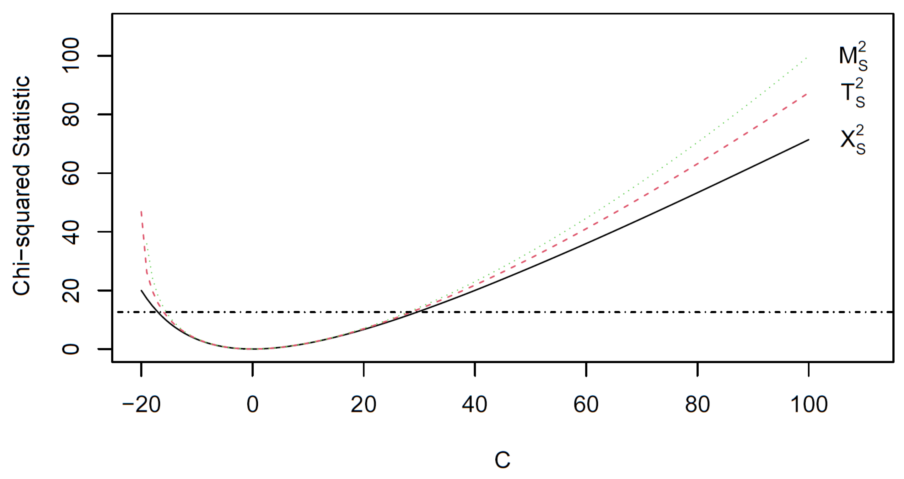
Figure 2.
versus for Table 1; and 0
Figure 2.
versus for Table 1; and 0
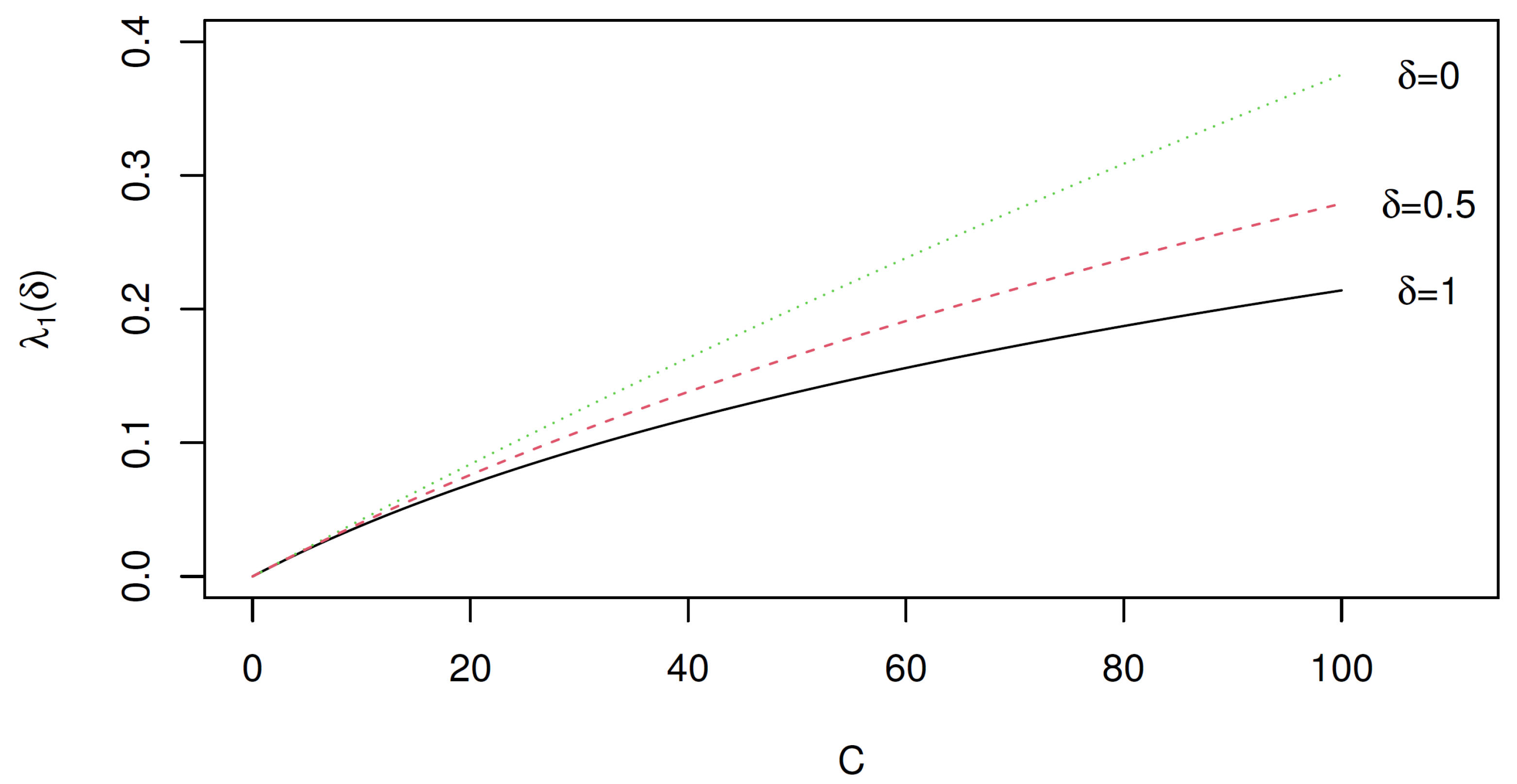
Figure 3.
versus for Table 1; and 0
Figure 3.
versus for Table 1; and 0
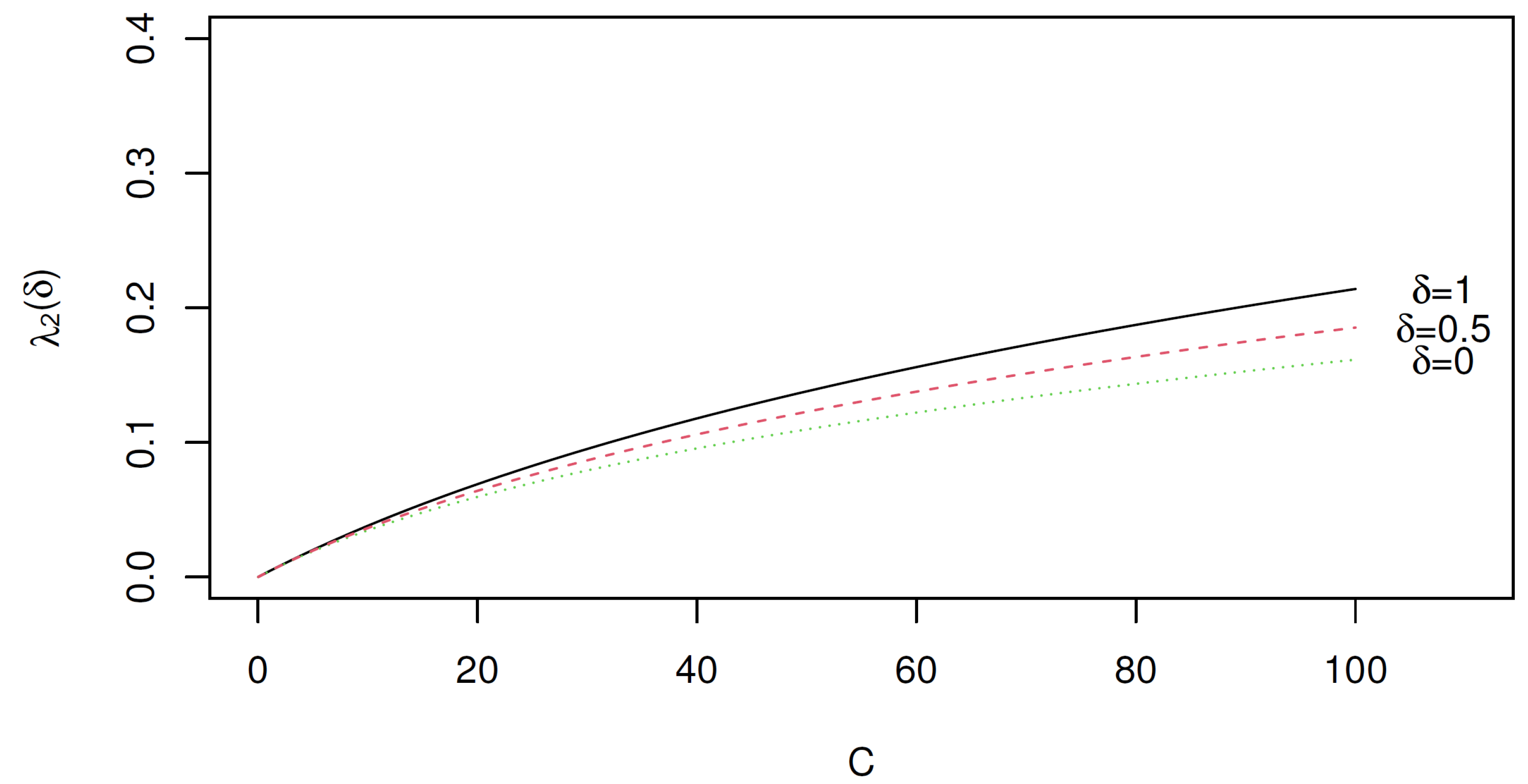
Figure 4.
versus for Table 1; and 0
Figure 4.
versus for Table 1; and 0
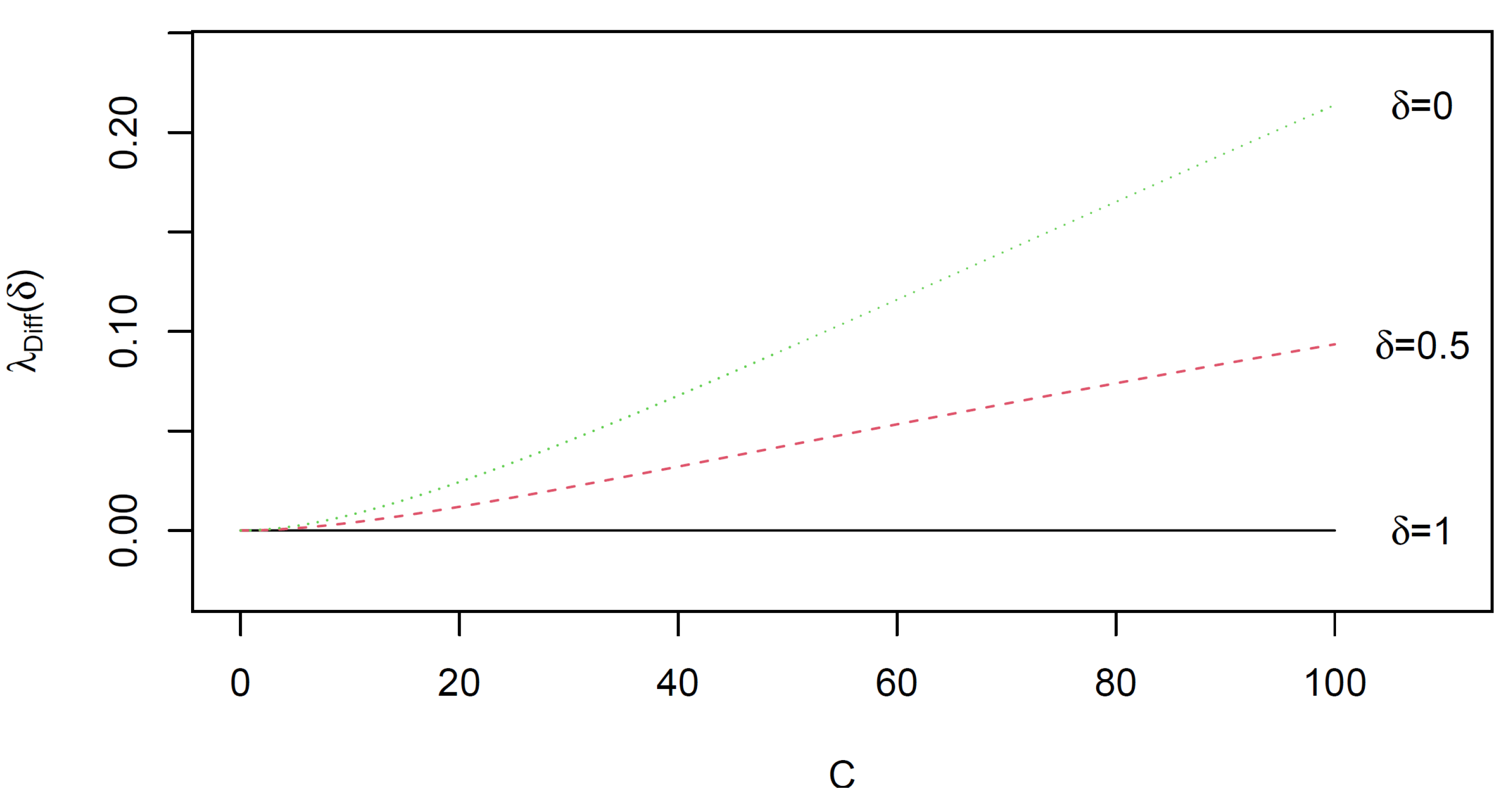
Figure 5.
Correspondence plot for Table 1 with where (a) , (b) and (c)
Figure 5.
Correspondence plot for Table 1 with where (a) , (b) and (c)
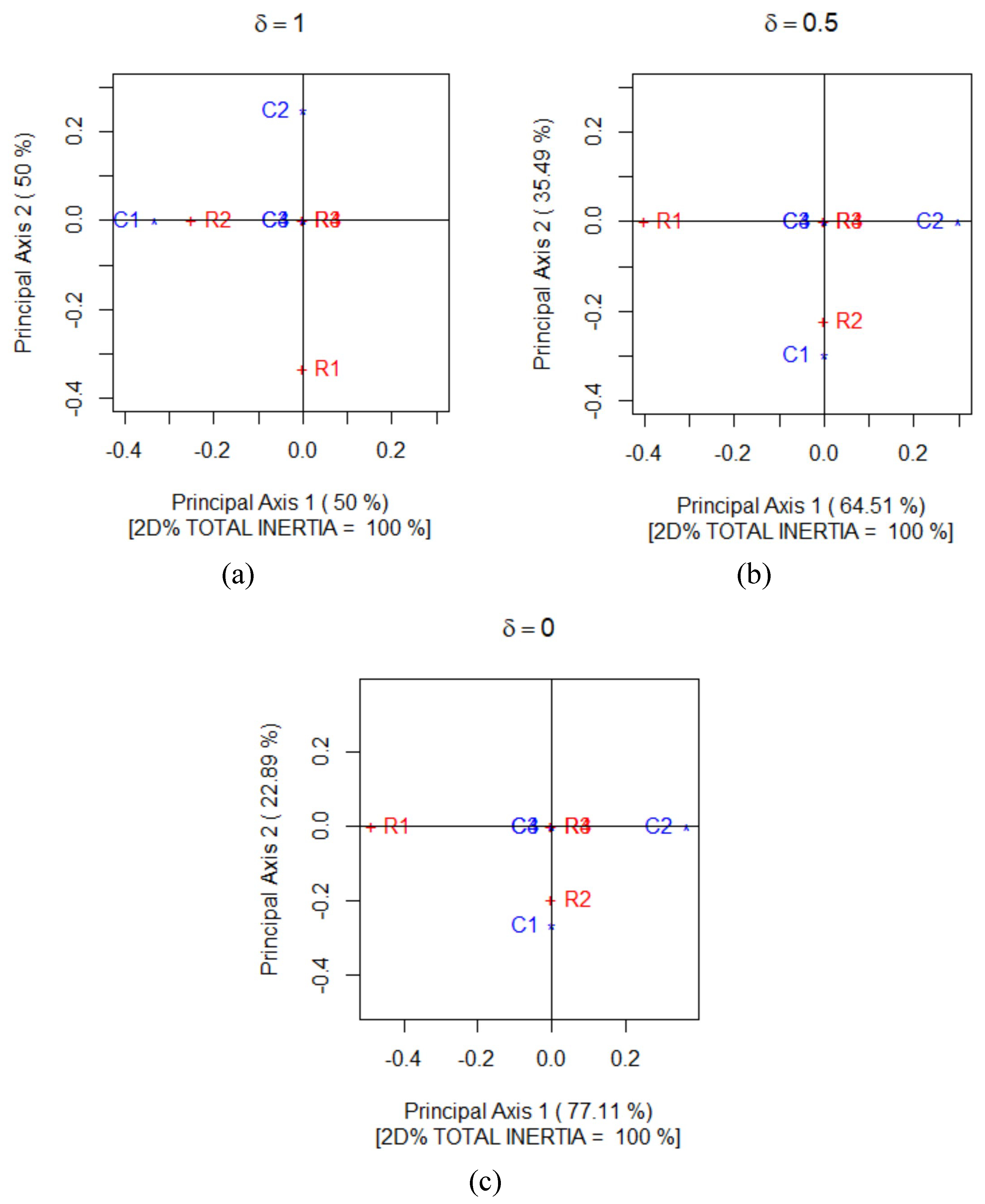
Figure 6.
Correspondence plot for Table 2 where (a) , (b) and (c)
Figure 6.
Correspondence plot for Table 2 where (a) , (b) and (c)
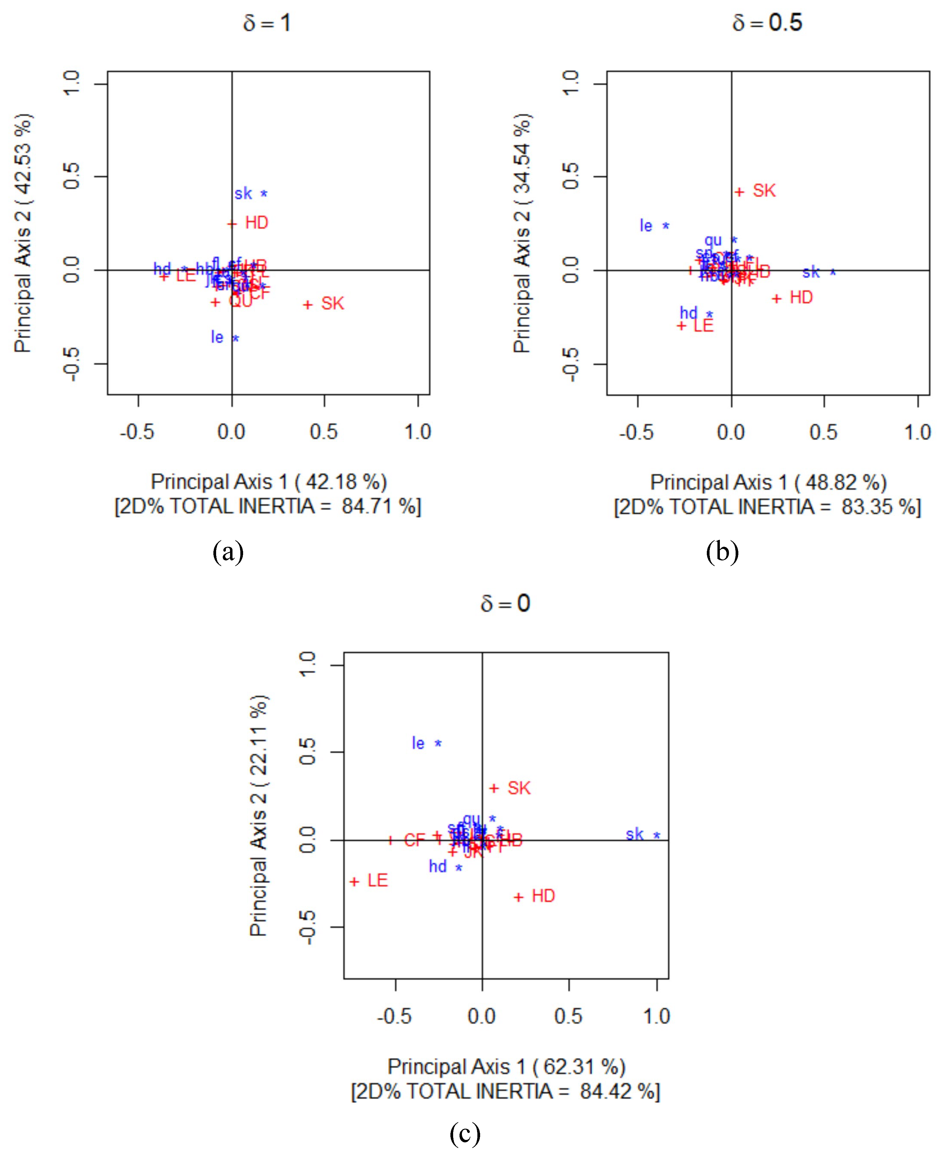

Table 1.
A near-symmetric artificial contingency table where C is a non-negative integer.
| Columns | |||||
|---|---|---|---|---|---|
| Rows | C1 | C2 | C3 | C4 | Total |
| R1 | 10 | 20 | 30 | 40 | 100 |
| R2 | 20 + C | 50 | 60 | 70 | 200 + C |
| R3 | 30 | 60 | 20 | 40 | 150 |
| R4 | 40 | 70 | 40 | 80 | 230 |
| Total | 100 + C | 200 | 150 | 230 | 680 + C |
Table 2.
The pre- and post-courtship behaviour of bitterlings (Rhodeus amarus Bloch, Source: [33] ).
Table 2.
The pre- and post-courtship behaviour of bitterlings (Rhodeus amarus Bloch, Source: [33] ).
| Pre-Courtship Behaviour | |||||||||||||
|---|---|---|---|---|---|---|---|---|---|---|---|---|---|
| Post- | jk | tu | hb | cs | fl | qu | le | hd | sk | sn | cf | ff | Total |
| JK | 654 | 128 | 172 | 56 | 27 | 25 | 1 | 28 | 0 | 46 | 14 | 18 | 1169 |
| TU | 101 | 132 | 62 | 27 | 5 | 1 | 1 | 11 | 0 | 8 | 5 | 9 | 362 |
| HB | 171 | 62 | 197 | 130 | 0 | 25 | 0 | 50 | 14 | 18 | 14 | 12 | 693 |
| CS | 60 | 22 | 152 | 135 | 0 | 8 | 0 | 43 | 16 | 15 | 12 | 4 | 467 |
| FL | 19 | 2 | 0 | 0 | 419 | 19 | 0 | 2 | 0 | 17 | 5 | 11 | 494 |
| QU | 36 | 1 | 18 | 5 | 12 | 789 | 119 | 295 | 26 | 70 | 1 | 14 | 1386 |
| LE | 4 | 0 | 0 | 0 | 0 | 57 | 167 | 73 | 0 | 8 | 0 | 0 | 309 |
| HD | 22 | 9 | 40 | 37 | 5 | 245 | 7 | 171 | 287 | 53 | 8 | 13 | 897 |
| SK | 3 | 2 | 7 | 38 | 0 | 120 | 8 | 134 | 19 | 28 | 4 | 9 | 363 |
| SN | 42 | 2 | 17 | 16 | 20 | 70 | 11 | 67 | 9 | 225 | 12 | 12 | 503 |
| CF | 18 | 3 | 10 | 13 | 6 | 5 | 0 | 8 | 0 | 24 | 97 | 9 | 193 |
| FF | 27 | 3 | 6 | 5 | 10 | 13 | 0 | 18 | 0 | 10 | 8 | 29 | 129 |
| Total | 1157 | 366 | 681 | 462 | 504 | 1377 | 314 | 900 | 371 | 522 | 180 | 131 | 6965 |
Table 3.
The matrix of divergence residuals, for and 0.
| Pre-Courtship Behaviour | |||||||||||||
|---|---|---|---|---|---|---|---|---|---|---|---|---|---|
| Post- | jk | tu | hb | cs | fl | qu | le | hd | sk | sn | cf | ff | |
| 1 | 0.015 | <0.001 | -0.003 | 0.010 | -0.012 | -0.011 | 0.007 | -0.015 | 0.004 | -0.006 | -0.011 | ||
| JK | 1/2 | 0.015 | <0.001 | -0.003 | 0.010 | -0.013 | -0.014 | 0.007 | -0.027 | 0.004 | -0.006 | -0.012 | |
| 0 | 0.014 | <0.001 | -0.003 | 0.009 | -0.013 | -0.017 | 0.007 | -0.074 | 0.004 | -0.006 | -0.013 | ||
| 1 | -0.015 | 0 | 0.006 | 0.010 | 0 | 0.008 | 0.004 | -0.012 | 0.016 | 0.006 | 0.015 | ||
| TU | 1/2 | -0.016 | 0 | 0.006 | 0.009 | 0 | 0.007 | 0.004 | -0.022 | 0.014 | 0.006 | 0.013 | |
| 0 | -0.016 | 0 | 0.006 | 0.008 | 0 | 0.006 | 0.004 | -0.056 | 0.013 | 0.005 | 0.012 | ||
| 1 | <0.001 | 0 | -0.011 | 0 | 0.009 | 0 | 0.009 | 0.013 | 0.001 | 0.007 | 0.012 | ||
| HB | 1/2 | <0.001 | 0 | -0.011 | 0 | 0.009 | 0 | 0.009 | 0.012 | 0.001 | 0.007 | 0.011 | |
| 0 | <0.001 | 0 | -0.012 | 0 | 0.008 | 0 | 0.008 | 0.011 | 0.001 | 0.006 | 0.010 | ||
| 1 | 0.003 | -0.006 | 0.011 | 0 | 0.007 | 0 | 0.006 | -0.025 | -0.002 | -0.002 | -0.003 | ||
| CS | 1/2 | 0.003 | -0.006 | 0.011 | 0 | 0.007 | 0 | 0.006 | -0.029 | -0.002 | -0.002 | -0.003 | |
| 0 | 0.003 | -0.006 | 0.011 | 0 | 0.006 | 0 | 0.005 | -0.033 | -0.002 | -0.002 | -0.003 | ||
| 1 | -0.010 | -0.010 | 0 | 0 | 0.011 | 0 | -0.010 | 0 | -0.004 | -0.003 | 0.002 | ||
| FL | 1/2 | -0.010 | -0.011 | 0 | 0 | 0.010 | 0 | -0.011 | 0 | -0.004 | -0.003 | 0.002 | |
| 0 | -0.011 | -0.013 | 0 | 0 | 0.010 | 0 | -0.013 | 0 | -0.004 | -0.003 | 0.002 | ||
| 1 | 0.012 | 0 | -0.009 | -0.007 | -0.011 | 0.040 | 0.018 | -0.066 | 0 | -0.014 | 0.002 | ||
| QU | 1/2 | 0.011 | 0 | -0.009 | -0.008 | -0.011 | 0.037 | 0.018 | -0.083 | 0 | -0.017 | 0.002 | |
| 0 | 0.011 | 0 | -0.010 | -0.008 | -0.012 | 0.034 | 0.017 | -0.106 | 0 | -0.023 | 0.002 | ||
| 1 | 0.011 | -0.008 | 0 | 0 | 0 | -0.040 | 0.063 | -0.024 | -0.006 | 0 | 0 | ||
| LE | 1/2 | 0.010 | -0.015 | 0 | 0 | 0 | -0.044 | 0.053 | -0.046 | -0.006 | 0 | 0 | |
| 0 | 0.009 | -0.034 | 0 | 0 | 0 | -0.049 | 0.046 | -0.144 | -0.006 | 0 | 0 | ||
| 1 | -0.007 | -0.004 | -0.009 | -0.006 | 0.010 | -0.018 | -0.063 | 0.063 | -0.011 | 0 | -0.008 | ||
| HD | 1/2 | -0.007 | -0.004 | -0.009 | -0.006 | 0.009 | -0.019 | -0.088 | 0.058 | -0.011 | 0 | -0.008 | |
| 0 | -0.008 | -0.004 | -0.009 | -0.006 | 0.008 | -0.019 | -0.132 | 0.054 | -0.012 | 0 | -0.008 | ||
| 1 | 0.015 | 0.012 | -0.013 | 0.025 | 0 | 0.066 | 0.024 | -0.063 | 0.026 | 0.017 | 0 | ||
| SK | 1/2 | 0.012 | 0.010 | -0.014 | 0.023 | 0 | 0.058 | 0.020 | -0.070 | 0.024 | 0.014 | 0 | |
| 0 | 0.010 | 0.008 | -0.016 | 0.021 | 0 | 0.051 | 0.017 | -0.079 | 0.021 | 0.012 | 0 | ||
| 1 | -0.004 | -0.016 | -0.001 | 0.002 | 0.004 | 0 | 0.006 | 0.011 | -0.026 | -0.017 | 0.004 | ||
| SN | 1/2 | -0.004 | -0.020 | -0.001 | 0.002 | 0.004 | 0 | 0.006 | 0.011 | -0.031 | -0.019 | 0.004 | |
| 0 | -0.004 | -0.024 | -0.001 | 0.001 | 0.004 | 0 | 0.005 | 0.010 | -0.037 | -0.021 | 0.003 | ||
| 1 | 0.006 | -0.006 | -0.007 | 0.002 | 0.003 | 0.014 | 0 | 0 | -0.017 | 0.017 | 0.002 | ||
| CF | 1/2 | 0.006 | -0.006 | -0.007 | 0.002 | 0.002 | 0.012 | 0 | 0 | -0.032 | 0.016 | 0.002 | |
| 0 | 0.006 | -0.007 | -0.008 | 0.002 | 0.002 | 0.011 | 0 | 0 | -0.090 | 0.015 | 0.002 | ||
| 1 | 0.011 | -0.015 | -0.012 | 0.003 | -0.002 | -0.002 | 0 | 0.008 | 0 | -0.004 | -0.002 | ||
| FF | 1/2 | 0.011 | -0.017 | -0.013 | 0.003 | -0.002 | -0.002 | 0 | 0.007 | 0 | -0.004 | -0.002 | |
| 0 | 0.010 | -0.020 | -0.015 | 0.003 | -0.002 | -0.002 | 0 | 0.007 | 0 | -0.004 | -0.002 | ||
Disclaimer/Publisher’s Note: The statements, opinions and data contained in all publications are solely those of the individual author(s) and contributor(s) and not of MDPI and/or the editor(s). MDPI and/or the editor(s) disclaim responsibility for any injury to people or property resulting from any ideas, methods, instructions or products referred to in the content. |
© 2024 by the authors. Licensee MDPI, Basel, Switzerland. This article is an open access article distributed under the terms and conditions of the Creative Commons Attribution (CC BY) license (http://creativecommons.org/licenses/by/4.0/).
Copyright: This open access article is published under a Creative Commons CC BY 4.0 license, which permit the free download, distribution, and reuse, provided that the author and preprint are cited in any reuse.


