Exploring Reduced Graphene Sheets RGo Stabilized by Cu(II) and Cu(I) Cations and Dispersed in Ethanol

Cu-ions dispersed on reduced graphene RGo prepared and characterized in a liquid state in ethanol. Either constant ultrasounds or a sequence of ultrasounds (15s working, 15s stop) were applied for 6 min or 2h overall time, at a power of 500 W. Commercial graphite in ethanol was introduced at a concentration of 0.04 g/mL and CuCl2 2.5 H2O concentrations between 0.012 and 0.04 g/mL were used. The structural characterizations performed by XRD, microscopic, and spectroscopic techniques, after a centrifugation at 5000 rpm applied 12 min before Cu-introduction, led to conclude that: 1) Without copper, negative peaks in UV spectra were detected with concentrated pure graphene solutions, indicating light emission as nicely confirmed next by fluorescence measurements, 2) After addition of copper chloride and equilibration for 2 min , very intense and narrow peaks of intensity larger than 10 were observed. These peaks due to collective excitations generating plasmons were suppressed at a higher dilution and also if the cell with one cm optical path was replaced by a narrower cell with a 0.2 cm path. When plasmons were suppressed, in the UV spectral range, a band gap due to the energy transition between the valence filled  orbitals and conducting empty * orbitals, was observed. The presence of Cu (II) and Cu (I) cations were evidenced by Visible NIR spectroscopy. The formed “green” liquors containing Cu (II) Cu (I) /graphene in ethanol were stable in air for months and had good photocatalytic visible properties as demonstrated by the decomposition of two dyes.

Keywords:

Photocatalysis

;

Cu2+ and Cu+

;

graphite

;

reduced graphene (RGo)

;

Ultrasounds

;

Plasmons

;

Dyes decomposition

Subject:

Chemistry and Materials Science - Materials Science and Technology

Supplementary Material

supplementary.pdf (288.08KB )

1. Introduction

Single or few layers 2D graphene sheets have excellent mechanical and optical properties. They are formed by carbon atoms arranged to form a honeycomb structure, defined by carbon atoms in a sp² hybridization, as described in a general public magazine in 2008 [1]. The word graphene has a beginning in graph- to recall carbons species. Its –ene end is associated to its polycyclic aromatic hydrocarbon’s nature [2]. The electrons inside the sigma bonds between the carbon atoms are stable. Extraordinary optical properties are due to the electrons inside the atomic 2p_z orbitals of the carbon atoms. These atomic orbitals are overlapped and extended valence bonding π and conducting anti-bounding π* molecular orbitals are formed. Intrabands and interbands electronic transitions in the spectral range UV, visible and Far Infrared are observed.

The introduction of graphene in photocatalysis was reviewed in 2016 [3]. Different methods for its exfoliation and to obtain 2D graphene particles of several dimensions and thicknesses were reviewed in ref. [4]. The UV-visible-NIR absorption spectra of reduced graphene particles is complex mainly because of electrons interactions. The first detailed general description of electrons interactions has been published in 1952 [5]. Localized surface plasmons have then been described in 2007 by Maier, S.A. [6]. Initial studies were devoted to metallic particles but possible application also to reduced graphene have been reported in 2014 [7,8,9]. With added copper chloride, RGo particles are associated with strong absorption, that can be called plasmons. Furthermore, if the graphene particles are suspended in a solvent, they have indirect semi-conducting properties and a band gap can be detected between their valence and their conduction bands. [10,11]. These bands positions in energy are strongly affected by the size and the shape of the graphene nanoparticles, as well as by their O-containing defects (OH, peroxide and carboxylic acid groups) and structural defects (C-vacancies). We have looked to plasmons and also to band-gap value in our samples prepared with CuCl₂ 3H₂O and reduced graphene obtained by ultra-sounds and dispersed in ethanol, the four questions which were now arising being:

1) is the added Copper chloride hydrated salt necessary to observe plasmons?

2) can we adjust plasmons positions and intensities by a simple dilution?

3) can we evidence the plasmons coupling with C-C vibrations?

4) can we eliminate s the plasmons to study photocatalytic properties that can be attributed to our Copper species and reduced graphene particles.

We will answer to these four questions, using a simple UV-visible-NIR spectra. In addition, small negative peaks are observed in the UV range and suggest that some emission of light, fluorescence also takes place, and can be due to copper and to graphene sheets. To clarify that point, and check that the fluorescence was due to the graphene sheets in themselves, measurements of fluorescence before the addition of copper have been made. Fluorescence results are then compared with published ones [12]. Two methods aimed at suppressing the plasmons, dilution or use of special cells with a 0.2 cm optical cell are compared. When plasmons are suppressed, band-gap measurements of C-species can be made using classical method [13] and the methods developed in our laboratory [13,14,15,16,17]. Obtained optical characterizations, band gap values, are compared to published ones [18,19]. Catalytic tests about two dyes, eosin and bromophenol blue decomposition, are finally introduced to follow the subject of dye degradation under visible light irradiation over copper.

We have acquired a commercial graphite containing 3D graphite particles and stable 2D nanoscrolls. Nanoscrolls are described and their practical use is details by several authors [20,21,22]. We have reported that ultra-sound technique can be used to exfoliate them and the 3D graphite GR particles to obtain flat particles and to use them after as supports for Zn-ferrite nanoparticles to eliminate antibiotic traces of an antibiotic, Amoxycillin [23]. In the most common preparation method using ultra-sounds, in water, oxidized GO sheets are obtained using the Hummer’s method. GO is then reduced to give RGo, and three distinct three distinct reducers have been used, hydrazine, ascorbic acid and natural extracts of Amaranthus hybrids [24]. Here, ethanol was used as solvent and also as a reducer [23]. The RGo symbol was kept to describe our reduced graphene containing samples, having a black color, even if no intermediate oxidized step was necessary to prepare them. Ultra-sound treatments to prepare graphene particles suspended in a solvent are common. Some of the reported data concern samples prepared indirectly, using ultrasounds in thermostatic beakers introduced in a water bath or a horn introduced inside the solution that can be water [25], ethanol [26] or water with strong mineral acids [27]. As made in refs 10 to 12, we have used a horn directly introduced inside the liquid solvent. More details about the three publications (power, frequencies, times of the ultrasound treatment are summarized in Supplementary Information).

Copper is an interesting metal, cheap and abundant. Solid catalysts containing isolated copper ions dispersed on porous nanocrystals of zeolite FAU or of Reduced graphene oxide for instance are interesting for oxidation reactions of oxygen and also for the degradation of pollutants [19,29]. The complexation of transition metal ions in the surface of graphene has been recently reviewed [30] and the grafting of copper yielding to Cu(I) isolated sites has been studied for instance in refs. [31,32]. Liquid Cu/Zn on graphene have also been formed by CVD [33]. To avoid graphene agglomeration, neutral surfactants and negatively charged species can be added. But simple addition of organics is affecting the physical-chemical properties of the graphene sheets. Here, similar solids are obtained by a simple contact of suspended graphene nanoparticles with mineral species Cu (Cl)₂ 3H₂O after an ultra-sound treatment aimed at eliminating the nanoscrolls of graphene and a centrifugation aimed at eliminating graphite 3D particles. Solids characterizations are performed by XRD, SEM and TEM micrographs, associated with Selected Area Electrons Diffraction. We will focus on the description of the plasmons intensities and positions as a function of the Cu/RGo dilution in ethanol. In addition, small negative peaks are observed in the UV range will suggest that some emission of light, fluorescence also takes place, and can be due to copper and to graphene sheets. To clarify that point, and check that the fluorescence was due to the graphene sheets in themselves, measurements of fluorescence before the addition of copper have been made. Fluorescence results are then compared with published ones [14]. Two methods aimed at suppressing the plasmons, dilution or use of special cells with a 0.2 cm optical cell are compared. We will see that plasmons and vibrations of the C-species are coupled. When plasmons are suppressed, band-gap measurements of C-species can be made using classical method [15] and the methods developed with our students [16,17,18] and with students of another group [19]. Obtained optical characterizations, band gap values, are compared to published ones [12,34]. Catalytic tests about two dyes, eosin and bromophenol blue decomposition, are finally introduced to follow the subject of dye degradation under visible light irradiation over Copper/ RGo.

2. Materials and Methods

2.1. Materials

Initial commercial graphite flakes, GR, are 99% Carbon, 100 Mesh, Natural from Sigma Aldrich n° 808091, CAS 7782-42-5. We used absolute alcohol CAS 64-17-5 and CuCl₂ 2.5 H₂O, CAS 10125-13-0 from the same society. All these reagents lack of intrinsic toxicity. We focused here on the work made with the catalysts in a liquid state, its dilution in ethanol. Graphene suspensions contained reduced graphene RGo and are easily recognized because of their black color. The ultrasounds treatment was applied directly inside centrifugation vials, to warrant the absence of unwanted contamination due to metallic species and ascertain that the containers always have the same shape and volume. The vials have a conical basic shape and a height of 115 cm. They contain between 40 and 45 mL of ethanol.

2.2. Methods

Scanning electron microscopy (SEM) imaging was performed with a Hitachi SU-70 FESEM. Transmission electron micrographs were registered on a JEOL JEM 2011 UHR (LaB6) microscope operating at 200 kV and equipped with an ORIUS Gatan Camera. For the observations, the liquids were deposited on 3 mm copper grids coated with an amorphous carbon film and let to dry.

Ultrasonic irradiations were generated by a Vibracell VCX 500 apparatus from Bioblock (500 W power, used at 40%, with a frequency of 20 kHz). The horn of this apparatus of 13 mm in diameter and was made with an alloy of Ti-6Al-4V, warranted for an overall volume of solution of 50 ml. The probe was penetrating by 6 cm inside the used liquid inside the vial. We have used either constant irradiations for 5, 6, 7 min or for 2 hours with and without pulses of 15s and stops of 15s. Experimental conditions, the influence of the ultra sounds power, several sonication times and of the initial graphite concentration GR were detailed for instance by Navik et al. [26]. The used initial concentration of graphite was equal to 5 mg/ ml, the sonication was realized in sonication bath with a power of 1.08 kW. The cited publication was devoted to graphene stabilization by an organic molecule, curcumin, stable for a graphene concentration of 1.44 mg/mL, but it was also containing complementary data concerning the detection of graphene sheets in ethanol with several initial GR concentrations. There is a main difference between these published results and ours, since the used ultra sound horn is penetrating deeply in solution.

In our liquors, to avoid solids precipitation, we have used 6 min or 2h of ultrasound treatment, and we have used concentrations of initial graphite GR introduced in concentrations lower than 0.5 mg/ml. After the ultrasonic treatment, a centrifugation was applied at 3000 and/or 5000 rotations by min, rpm, 12 min. Bulk 3D graphite was recovered at the bottom of the flask. It contains a lot of 3D graphite (demonstrated by SAXS measurements, Figure S1) and was eliminated. The transparent black liquor was then used directly to dissolve the salt, copper chloride trihydrate. The solution was changing of color spontaneously and became green in less than 2 min. We were surprised to observe that the green color of the solution was extremely stable, remaining constant even after several months of storage in air, whereas the species that we have detected that can be green are Cu (I) cations and are known to be instable so that only the redox potential of the couple Cu (II) Cu (metal) is given in books. To explain their stability, a positive role of ethanol to protect them is proposed.

The presence of the graphene sheets in suspension in ethanol was studied first by WAXS Wide Angle Scattering. WAXS measurements were made on a Bruker type D8 Advance within the range 2θ from 0.3 to 90 with a copper 1.54186 Å, with a mixture of Kα₁ and Kα₂, with a ratio of 1 for 2. A Bragg Brentano set-up was used to obtain graphics in intensities versus 2θ. Simulations were made using the Fullprof program. With this program, precise values of peaks positions and intensities (integrated units) were obtained. Within the range 23-31°, three observed peaks were labelled (1), (2) and (3). (1) is a small peak on the left part. Peaks (2) and (3) are more than 5 times more intense and are on the right part. Two additional peaks attributed to X-ray diffusion are presented in Figure S2 about the shape of the diffraction peaks (2) and (3) were calculated, based on two parameters H = FWHM, the Full-Width at Half Maximum and ETA, η, that was a linear combination of a Lorentzian L and a Gaussian G line-shapes with the same FWHM.

η = η_{0} + 2 θ X = η L + (1 - η) G,

(1)

A value of η close to zero is indicating a Gaussian line shape. Intermediates values between 0 and 1 indicated a pseudo-Voigt shape with given % of G(x) and L(x). Numerical correct expressions of the integration of L(x) and G(x) functions between

23 a n d 31 °

as a function of x = 2θ, with

x_{0}

corresponding to the peak maximum, can be written:

Gaussian:

G (x) = \int_{+ 23}^{+ 31} e^{{- x}^{2}} d x

(2)

Lorentzian:

L (x) = \int_{+ 23}^{+ 31} \frac{H}{2 π} \frac{1}{\frac{H^{2}}{4} + {(x - x_{0})}^{2}} d x

(3)

Two very small diffraction peaks associated with X-ray diffusion are located at the same positions than peaks (2) and (3) and are labelled peaks (4) and (5) (Figure 1).

UV-visible-NIR spectra were measured on a Varian 4000 spectrometer within the range 200-1400 nm. They were measured in the UV (200 to 400 nm), the visible (400 to 800 nm) and the NIR ranges inside two kinds of quartz cell, one in quartz with an optical path of 1 cm and a second with an optical path (internal) of 2 mm. Fluorescence measurements were made with a Horiba Jobin Yvon spectrometer Fluorolog®FL3-22. We have tried two kinds of fluorescence measurements. We have tried two kinds of florescence measurements, the first one with diluted solutions in ethanol and the second one directly with the concentrated initial solutions obtained by applying ultrasounds 6 min and without centrifugation.

The amount of graphene dispersed in absolute ethanol was determined by comparing the weight of an Eppendorf of 4 mL filled with several volumes of dilution (see details in the text) before and after ethanol evaporation.

Better results in fluorescence were obtained on the non-diluted solutions and for an angle between excitation light and detector set at 90° to avoid detector saturation.

3. Results

3.1. Solid Graphite GR, XRD to Study Mixture of Nanoscrolls and 3D Graphite

In XRD, enlargements between 23 and 31° were performed and analyzed with the program Fullprof. The positions of peaks (2) and (3), labels being indicated in the experimental part, are equal to 26.208 and 26.427° with respective FWHM values of 0.495 and 0.179° and for ETA values both equal to zero. The two peaks are then Gaussian in shape. Peak (3) is the narrowest and can be assigned to 3D graphite (Figure 1).

Particles sizes can be estimated using Scherer equation in the following form:

L_{h k l} = \frac{0.9 λ}{{F W H M}_{h k l} c o s θ}

(4)

where FWHM = β is expressed in radians. Average particles sizes of 700 and 300 Å are obtained on peak (2) and (3). These dimensions are too large for nanoparticles (Figure 1)

Peak (2) is attributed to graphene sheets, their varied sizes being associated with a large FWHM of this peak, significantly larger than the one of peak (3), attributed to graphite 3D particles. It is interesting to know that this decomposition of the X-ray diffraction peak is no longer detected when the GR commercial sample is submitted to an ultra-sound treatment after its suspension in ethanol, for 2h. In that case, a single XRD peak at 26.54° with a Gaussian shape that corresponds to the 002 diffraction of reconstructed 3D graphite domains is observed. The integrated intensities of the peaks (1), (2) and (3) indicate that the percentage of 3D graphite is 60.52% and the one of graphene, stabilized in nanoscrolls, of 36.33%.

3.2. Observations Correlated to Graphene Particles Sizes

3.2.1. Measurements Performed on SEM and TEM Images

The presence of the initial graphene nanoscrolls is evidenced on SEM images. They are formed by the scrolling of single layers of large graphene sheets (Figure 2). These nanoscrolls are decomposed after a simple manual grinding. Their diameter, as measured on adjacent nanoscrolls is of 235 nm. The commercial power also contains crystallized 3D graphite particles. A correct evaluation of the two solids is difficult on SEM images only, because only a given part of the sample is visible. But relative percentages of the two phases can be obtained using the XRD measurements.

After an ultrasound treatment of 6 min with pulses of 15s and stops of 15s, the nanoscrolls are no longer detected neither by microscopy, nor by XRD. The fact that nanoscrolls can be transformed in flat domains was already known, bubbles of cavitation being inserted within the main part of the scrolls and destroying them [21]. The present work complements previous studies by showing that the size of the flat nanoparticles is directly affected by the time of the applied ultrasound. μm size particles observed after 6 min of ultrasounds and drying are replaced by smaller particles, of size lower than 100 nm after ultra-sounds 2h as shown in Figure 3 on a TEM image. On the enlargement presented in Figure 4, several nanoparticles of copper oxide are seen aggregated and above the carbon surface, probably of a 3D particle of graphite of important size (more than 25 layers). A distance between fringes of 1.195Å can be measured. This distance is confirmed by a Fourier mathematical transformation and it is difficult to identify an inorganic species with one value only.

An additional Selected Electron Diffraction is presented in Figure 5 and was made on a graphene sheet. This image is important to establish that the studied specific sheet contains 5 distinct layers. The white spots are indeed grouped by 3 on the Bragg rings but the medium spot is larger than the 2 other ones.

These SEM and TEM images analysis were important to evidence 2D graphene thin (5 layers) mixed with more thick ones and also with 3D graphite. The information about the copper species is difficult to analyze since a dehydration was necessary and was performed before the introduction of the samples inside the TEM apparatus.

3.2.2. UV Visible-NIR Spectroscopy

3.2.2.1. Before Copper Introduction

The measured absorbance was used to estimate the concentration of graphene sheets in suspension. We used the Beer Lambert relation: A = ε c l and a cell with an optical path of l = 1 cm. The absorbance A has no units. C is the graphene concentration and ε their absorption coefficient in l. mol^-1.cm^-1.

Measurements were performed on two solutions, recovered after ultrasounds treatments of 6 min, and realized one with and one without pulses of 15 s for progressive dilutions in absolute ethanol. Four points corresponding to dilution by a factor of 0.10 to 0.35 were used and initial concentration was 500 mg of graphite commercial in 45 mL of absolute ethanol. Navik and Gai [9] (b) have proposed for curcumin stabilized in water solutions of graphene, a preliminary value of (ε ∗c), of 1650 mL/mg for graphene suspensions in water. The same value cannot be used here since water is replaced by ethanol.

We present in Figure 6, the absorbance that can be measured after mixing several volumes of the activated solutions just after ultra-sounds treatment 6 min and centrifugation at 5000 rpm 12 min with and without pulses. The two solutions are black and a dilution by absolute ethanol is necessary before to measure the absorbance on a flat straight line between 700 and 800 nm.

Two times more graphene is formed with pulses. The corresponding overall amount of C-species in solution was determined in Eppendorf open and let to evaporate. No difference was measured with the two solutions made with 1000 and 750 μl, with pulses, mass of 0.062 mg and 0.0605 mg of Carbon were found. With the solution at 500 μl, the weight of carbon was equal to 0.0417 mg. Converted in μg by ml (with 4 ml total volume, this gives 15.5, 15.1 and 10.4 μg by ml of the diluted solution.

In practice, as detailed previously dilution was necessary before to collect the UV visible spectra. The necessary dilutions were performed taking Eppendorf of 5 mL containing 250 μL of the selected “green” liquor taken with a high precision manual Eppendorf pipette BIOHT Proline 100 – 1000 μL, calibrated at 1% of precision for 500 μL at room temperature (with a balance of precision 0.001 g) and letting them dry in an autoclave at 60°C, 2h. The weight of sample before and after drying was measured with a Mettler- Toledo (XPR204S maximum capacity 210 g, readability 0.1 mg) was given after ethanol evaporation, the final measured weight of solid, being due to the carbon contribution in the solution.

In Figure 7, a straight line is observed for the absorbance as a function of the detected C-species in the flask containing the solution after ethanol evaporation. the linearity is better when the observed absorbance is plotted as a function of the concentration of carbon expressed in μg by ml. This line was used after to estimate the

C-amount in our ethanol solutions (without dilution).

If the point corresponding to 1000 μl of the solution prepared with 6 min of ultrasounds and pulses of 15s is used, it corresponds to 11.5 μg of C-species by ml and then there are 0.52 mg of suspended C-species in the 45 ml of ethanol initial. Since we start with 500 mg of GR, this corresponds to a low percentage, only 0.1% of the introduced C-species. Direct comparison with results published by Navik [10] (b) that concern ultrasounds applied with a horn, as we have made, is possible an amount of C-species in ethanol of 1.36 mg by ml, more than two times larger than ours, was obtained. The better obtained result was assigned to the use of curcumin large organic molecules that stabilize the graphene sheets. The power of the used ultra-sound treatment was equal to 0.18, 0.54, 1.08 and 1.8 W in that publication and we have used 40% of a power of 500W, 200W, more than 20 times more power. Despite the higher power that we have used, our graphene suspension in ethanol was lower. More than the ultrasounds power, this difference can then be assigned: 1) to curcumin, 2) to the used initial 3D graphite, its weight being equal to 50 mg by ml in this publication and equal to 500 mg in 45 ml in our case, lower 11.11 mg by ml, 3) to the time during which the ultra-sound treatment is applied is also important. It was of 4h in the publication and we have used 6 min.

3.2.2.1. b) After Copper Chloride Addition

After a first centrifugation at 3000 rpm 12 min, the solution is recovered and the solid CuCl₂ 2 H₂O salt is added, the salt is fully dissolved in less than 2 minutes and the liquor exhibits a “green” homogeneous color. This treatment has been reproduced with centrifugation at 5000 rpm 12 min.

After addition of CuCl₂.2H₂O, three distinct kinds of vibrations are observed: 1) in the UV range, vibrations of the C-C, C=C bounds of graphene and graphite, 2) between 300 and 400 nm, very intense vibrations, due to collective excitation, plasmons of intensities greater than 10, 3) above 800 nm, vibrations of octahedral (tetrahedral Cu-complexes possible also).

On the right part of the visible spectrum recorded with our more concentrated solution, one broad at 866 nm and a second one at 930 nm. Figure 6 is presenting the spectra recorded as a function of the dilution in ethanol. An observed broad peak due to stable species corresponds to three peaks because of the axially distorted octahedral crystal field formed by 6 water molecules around the Copper cations. This distortion occurs because of the Jahn Teller effect in the hexa-aqua [Cu (H₂O)₆ ]²⁺ complexes. The value of the Δ^O parameter which characterize the electrons d-d transition in Cu (II) complexes is slightly too high to corresponds to a Jahn Teller effect. The average position of the observed peak is indeed shifting from 800 nm for a hexa-aqua complex to 866 nm. The observed important distortion can be attributed to the exchange of 2 water molecules by ethanol. Indeed, no ethanol/water exchange by 3 molecules is possible, as demonstrated an old ESR study [34]. We will confirm that point in the future on our samples... There is also a broad absorption that is observed at 930 nm on the spectrum of the most concentrated solution spectrum (Figure 6 (c)). Because of its position this signal is attributed to Cu(I) species, possibly grafted on the graphene surface. They are stable toward an oxidation by air, by oxygen molecules. Some protection by the solvent, is necessary to explain their stability. Similar kinds of Cu-species, grafted on C-vacancies of carbon species on solid carbon diamond were very recently been evidenced [9,29,34]. They were investigated by demanding and expensive methods, EXAFS-XANES [29], but also by less expensive operando IR measurements [18]. Here, we have selected to use UV-visible-NIR spectroscopy.

In the left part of the spectrum, still with a concentrated solution, multiple and very intense peaks were detected between 309 and 371 nm (4.01 to 3.81 eV) with a second non resolved broad peak between 262 and 371 nm. By progressive dilutions, the narrow and intense peaks are eliminated and the first peak is decomposed in at least 3 peaks, one at 230 nm and two above 250 nm. By even more dilution, the broad peak with one component is shifting to 265 nm, position reported for thin reduced graphene. This position can be attributed to the π−π* electronic transition and is demonstrating the absence of GO in our diluted samples. For oxidized samples, a first peak value close to 230 nm was reported. The intense additional peaks were attributed to plasmons associated with light reflection by graphene suspended nanoparticles. We have observed that a simple dilution can eliminate their very intense peaks. A very similar result is obtained by changing the thickness of the used cell, going from 1 cm to an overall path of 2 mm internal (and 4 mm external). As illustrated in Figure 8 (a) and (b), in the two cases, the intense reflections are eliminated.

a): In black, preparation with 0.269 g graphite commercial GR; 45 mL absolute ethanol; ultra sounds 7 min and pulses of 15s.
b): In blue, dilution “1”: inside the UV cell, few drops inside 4 mL of absolute ethanol
c): In pink, dilution 2: 1 ml of dilution “1” diluted by 3 mL ethanol (inside the visible cell)

In our samples, it is not true that graphene has a zero band-gap because of the used dispersion in a solvent. A band-gap, difference in energy between its valence and its conduction band, is seen just after the plasmons in the UV range and its value is calculated here at the intersection between the most vertical line observed when going from 365 to 400 nm and the Ox axis and its conversion in energy (eV), spectra indicate a shift from 3.09 to 3.39 eV if the plasmons contribution is removed. In the orange spectrum, coupling between them and the natural vibrations of graphene, its C-C, C=C bounds is evidenced. Coupling between the added copper species and the plasmons is also demonstrated by the position of the broad peak due to the [Cu (H₂O)₆]²⁺ complex which is shifting from above 850 nm down to its usual value circa 800-810 nm with the dilution.

Reduced graphene is a semi-conductor and its band gap can be estimated after conversion of the Ox axis of the visible spectra in energy (E = (h. c)/λ, with h, the Planck constant, c the celerity of light in vacuum and λ, the light wavelength; obtained in eV, the value is then converted in Joule and gives 1238/λ); with graphene highly diluted in ethanol solutions. On TAUC plots, representing (E*α) power 0.5 versus the energy in eV, straight lines are obtained. The corresponding band gap for an indirect semi-conductor is obtained by calculation of the intercept of the lines with the Oy axis divided by the slope. An in- direct value of 4.08 eV is obtained for the sample obtained with 6 min of ultra-sounds. A value of 4.40 eV is obtained with the sample submitted to 2h of ultrasounds. The indirect value can be compared with the range between 4.7 eV (for a free-standing sheet of graphene) and 7.0 eV (graphite 3D) for a plasmon (collective) π - π* interband transition as proposed and calculated by Politano and Chiarello in 2014 [35].

For a given concentration, there is a small peak at 230 nm on Figure 9, observed only with the smallest thickness path cell. This peak is due to a contamination by oxidized C-species that can be OH, peroxide or COOH groups. At the highest concentration a superposition with a negative absorption is observed and the negative peak is masking traces of oxidized species. When the negative peak is present, no information about the oxidized species is available. After the elimination of the strong plasmons, only a maximum of absorption is observed at 270 nm in Figure 8 and can be attributed to the reduced graphene sheets, without coupling with the others vibrations. They are composed of C-atoms hybridized sp², forming closed domains which sizes are clearly evidenced by the presented UV spectra.

Care is necessary before to use this value. Indeed, in old publications, the graphene sheets were in general considered to have a zero band-gap. It is obviously not the case here since we are studying graphene sheets dispersed on a solvent. In ethanol and if plasmons are suppressed, we observe a very strong absorption in the UV spectrum and the existence of a band-gap in energy will be then confirmed by fluorescence spectra, as investigated next. We will just insist on the fact that the measured band gap energy can be measured using the Tauc expression recommended for indirect semi-conductors. A value of 3.67 eV is obtained with the larger graphene particles obtained after 6 min of ultra-sounds (Figure 10). Small sheets obtained after 2h of ultra-sounds are giving a larger energy value, of 4.02 eV because of a smaller number of involved C-atoms and a less efficient π delocalization.

BG in reduced graphene is given at 3.90, 3.60, and 3.20 eV for nanoparticles obtained by reduction of GO [31,32], the decreasing value being associated with differences of thicknesses. We assume that our two values 4.02 and 3.67 eV are rather associated with the dimension of our graphene particles

3.2.4. Influence of Graphene Sizes Studied by Fluorescence (Emission) Spectra

We have tried two kinds of florescence measurements, the first one with diluted solutions in ethanol and the second one directly with the concentrated initial solutions. Better results were obtained without dilution and for an angle excitation light–detector set at 90° to avoid detector saturation.

The fluorescence spectrum of reduced RGo dissolved in water, benzene, toluene, ethyl acetate, acetone, with an excitation pulse of 300 nm was already published [34]. It was demonstrated inside this publication that the fluorescence indeed exists and that the fluorescence properties were strongly affected by the solvent polarity. Ethanol polarity is larger than the one of acetone, a free OH group is also offering the possibility of H-bounds and we were therefore expecting to find a fluorescence signal.

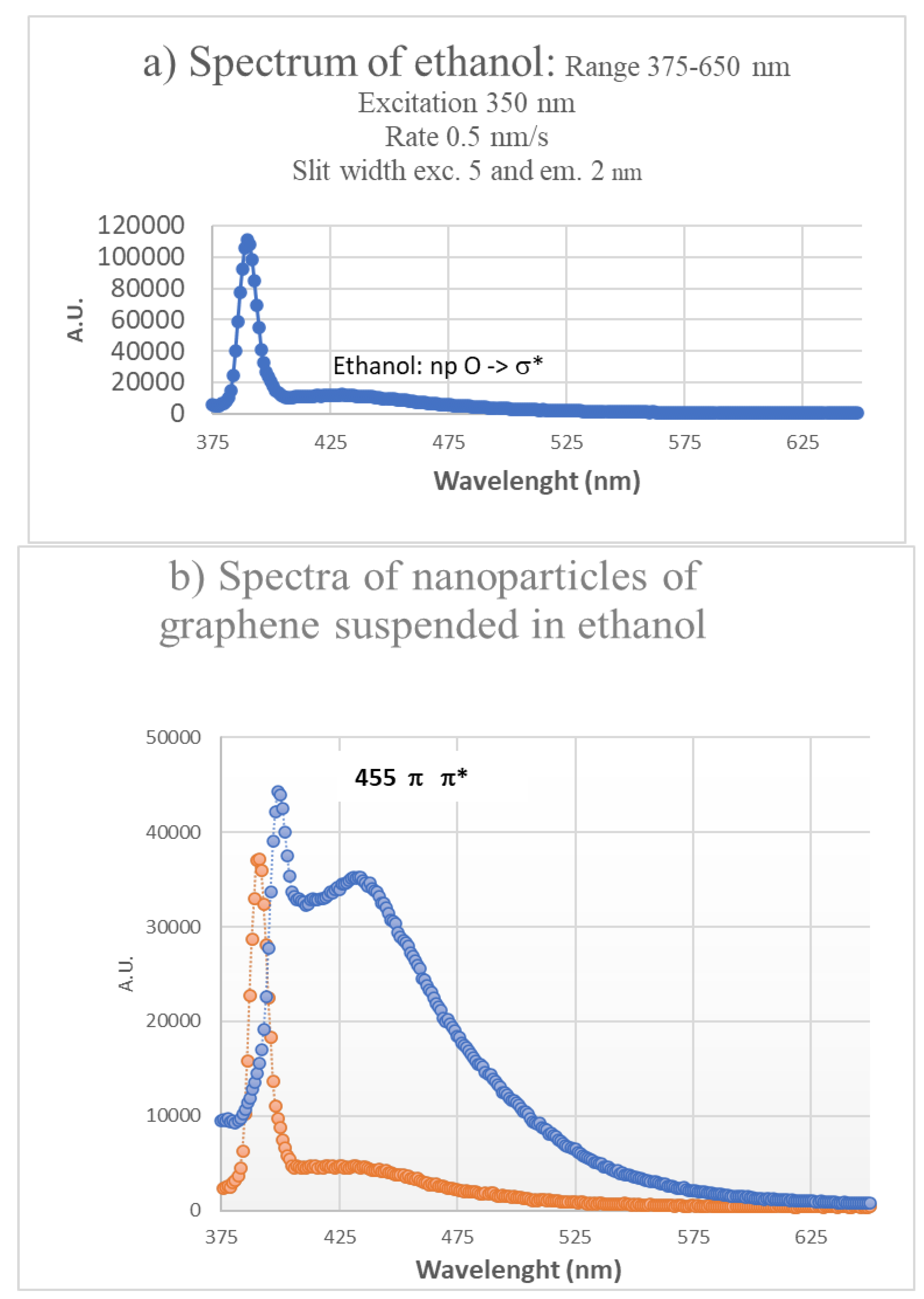
The detected fluorescence signals are presented in Figure 11 (a) ethanol and (b) two spectra recorded on the small particles of graphene obtained by a 2h ultrasound treatment and with ultrasounds 6 min

The signal keeps a detectible intensity between 400 and 625 nm. The fluorescence spectrum of RGo dissolved in water, benzene, toluene, ethyl acetate, acetone at the excitation pulse of 300 nm have already been reported. The signal detected here in ethanol is stronger with the larger graphene nanoparticles obtained with 6 min of ultrasounds than after 2h of ultra-sounds. Its maximum shifts from 425 to 455 nm if the graphene particles size increases from micron sizes to lower than 100 nm in SEM and TEM images with less involved C-atoms and a lower energy π delocalization. The two measurements were performed with the same excitation 358 nm, the same rate of 1 nm by s and the same slit width, external of 5 nm and internal of 2 nm.

3.2.5. Reactivity Test

UV visible spectra were necessary to follow two organics dyes (eosin and bromophenol blue) oxidation. With eosin, the used initial concentration of the dye was equal to 44 mg inside 100 ml of distilled water. Dilutions were then made and necessary to collect UV visible NIR spectra:

1) 250 μL of the initial solution was diluted in 4 mL of distilled water, directly inside a 1 cm cell in quartz,

2) dilution 2 by dilution of 250 μL of dilution 1 into 4 mL of distilled water,

3) dilution 3, 250 μL of dilution 2 into 4 mL of water. To these dilutions, 250 μL of liquid was removed and replaced by 250 μL of the active liquor.

With the three solutions, the characteristic peaks of the eosin dye, were located at 503 and 534 nm, with relative absorbance of 0.503 and 1.15 for dilution 3. The three peaks were eliminated in seconds with a few drops of the active green liquors that we have tested both with small and with large RGo particles. A similar treatment was made with a blue bromophenol dye in water. The treatments were also reproduced in ethanol.

It is important to know that at the used dilutions, no plasmons of RGo were expected to be present. This was made on purpose to study the materials photocatalytic activity in their absence.

Conclusions and Perspectives

Ultra-sound treatments of ethanol dispersions of a commercial graphite (GR) were very efficient to obtain reduced and “flat” graphene sheets that we have characterized by XRD, SEM, TEM. UV-visible-NIR results were complemented by fluorescence spectroscopy. For ultrasounds at a power of 500 W (used at 40% and with a frequency of 20 MHz) treatments were made with a horn directly introduced inside the solution and were performed either in a constant method or using pulses of 15s, stops of 15s, for overall times of 5- 7 min and of 2 h.

Thanks to the systematic use of centrifugation vials having the same volume (45 mL), of solvent, the same amount of commercial graphite GR, and similar centrifugation conditions, we can conclude that the graphene sheets dimension was directly affected by the time of the used ultra-sound treatment. The main dimension of the graphene particles was decreasing from larger than a micron (ultrasounds of 6 min) to smaller of 100 nm (after ultrasounds 2h). Even after 2h of ultra-sound treatment, the C-particles remained stacked, more than 5 to 25 sheets were detected.

Interesting plasmons (collective excitation of electrons, considered as a gaseous plasma) were observed after centrifugation and addition of CuCl₂ 3H₂0 and both their intensities (absorption that can be larger than 10) and their positions were affected by dilutions. The existence of a coupling between the plasmons and the vibrations of the C-lattice was demonstrated. At a high dilution to remove the plasmons, the prepared Cl/Cu/graphene solutions were very strong oxidants as demonstrated by catalytic tests performed with a dye (eosin and blue of bromophenol in water and in ethanol). In our experimental conditions, the visible signal of the dye was indeed eliminated in a few seconds with both small and large RGo particles.

In the future, more concentrated solutions will be used to preserve plasmons. A more complete study including several solvents of varied polarity and using atomic force microscopy to study, molecular interactions between Copper, RGo and added organic molecules and to study process dynamic will be proposed.

Supplementary Materials

The following supporting information can be downloaded at the website of this paper posted on Preprints.org.

Acknowledgements

We would like to thank Mohamed Selmane, David Montero and Dalil Brouri working at Sorbonne University for their help in the measurements of X-ray diffraction at small and large angle, SEM and TEM measurements. SEM & EDS funded by Sorbonne Université, CNRS and Région Ile de France. Thanks to the Fédération de Chimie et de Matériaux de Paris Centre (FCMat) for using the X-ray diffusion and diffraction plateform and the electronic microscopes. The current Director, Vincent Vivier of the Laboratoire de Reactivité de Surface, Sorbonne Université and all the technical staff of the Laboratory of Surface Reactivity in Sorbonne Université are also acknowledged

Funding

This research did not receive any specific grants or funds.

Data Availability Statement

There is no additional data. The original contributions presented in the study are included in the article.

Conflicts of Interest

The author declares no conflicts of interest.

References

Fuchs, J.N. ; Goerbig, M.O. le graphène premier crystal bidimensionnel, Pour la Science, Physique, 2008, 367. 1-9.
Mbayachi, B.; Ndayiragije, E.; Sammani, T.; Taj, S.; E. Mbuta, R.; Khan, A. U. Graphene synthesis, characterization and its applications: A review, Results in Chemistry, 2021, 3, 100163. [CrossRef]
Li, X.; Yu, J.; Wageh, S.; Al-Ghamdi, A.A.; Xie, J.Graphene in Photocatalysis: A Review. Small., 2016, 12(48), 6640-96.
Minzhen, C.; Thorpe, D.; Adamson, D. H.; Schniepp. H. C. Methods of Graphite Exfoliation. Journal of Materials Chemistry, 2012, 22 (48) 24992. [CrossRef]
Ikram, M.; Sarfraz, A.; Aqeel, M.; A.U-H; Imran, M.; Haider, J.; Haider, A.; Shahbaz, A.; Salamat, A. Visible-Light-Induced Dye Degradation over Copper-Modified Reduced Graphene Oxide, Journal of Alloys and Compounds, 2020, 837. 155588. [CrossRef]
Grasseschi, D.; Silva, W.C.; Souza Paiva, R.D.; Starke, L.D.; Do A.S. Nascimento, Surface coordination chemistry of graphene: Understanding the coordination of single transition metal atoms, Coordination Chemistry Reviews, 2020, 422, 21346.
Huang, F.; Deng, Y.; Chen, Y.; Cai, X.; Peng, M.; Jia, Z.; Xie, J.; Xiao, D.; Wen, X.; Wang, N.; Jiang, Z.; Liu, H.; Ma, D. Anchoring Cu₁ species over nanodiamond-graphene for semi-hydrogenation of acetylene, Nat Commun, 2019, 10, 4431.
Zhang, L. ; Yang, X. ; Yuan, Q. et al. Elucidating the structure-stability relationship of Cu single-atom catalysts using operando surface-enhanced infrared absorption spectroscopy. Nat Commun, 2023, 14, 8311. [CrossRef]
Li, L.; Li, M.; Zhang, R.; Zhang, Q.; Geng, D. Liquid Cu–Zn catalyzed growth of graphene single-crystals. New J Chem. 2023, 47(45):20703-7.
Tabaja, N.; Brouri, D.; Casale, S.; Zein, S.; Jaafar, M.; Selmane, M.; Toufaily, J.; Davidson, A. Use of SBA-15 silica Grains for Engineering Mixtures of Co Fe and Zn Fe SBA-15 for Advanced Oxidation Reactions under UV and NIR, Applied Catalysis B: Environmental, 2019, 253, 369–378. [CrossRef]
Chettah, W.; Barama, S.; Medjram, M.-S.; Selmane, M.; Montero, D.; Davidson, A.; Védrine, J.C. Materials Chemistry and Physics, 2021, 257, 123714. [CrossRef]
Ghazinejad, M.; Hosseini Bay, H.; Reiber Kyle, J.; Ozkan, M. SPIE proceedings, 2014, Vol. 8994, 169-175. 0277786.
Jubu, P.R.; Yam, F.K.; Igba, V.M.; Beh, K.P. Tauc-plot scale and extrapolation effect on bandgap estimation from UV–vis–NIR data – A case study of β-Ga₂O₃, Journal of Solid State Chemistry, 2020, 290, 121576.
Tabaja, N. Nanoparticules d’oxydes de fer et de ferrites obtenues par nano-réplication : Réactivité chimique et application en dépollution des eaux, PhD Thesis, 2015, Paris, France. https://theses.fr/070382972.
Jezzini, A. ZnFe₂O₄ for Heterogeneous Photocatalysis in the Visible Spectrum, PhD Thesis,2020, Sorbonne Université, Paris, France.
Shenoy, R.U.K.; Rama, A.; Govindan, I.; Naha, A. The purview of doped nanoparticles: Insights into their biomedical applications, OpenNano, 2022, 8, 100070. [CrossRef]
Larin, G.M.; Minin, V.V.; Levin, B.V. and Buslaev, Y.A. Complexation in the CuCl₂_C₂H₅OH_H₂O System N. S. Kurnakov Institute of General and Inorganic Chemistry, Academy of Sciences of the USSR, Moscow. Translated from Izvestiya Akademii Nauk SSSR, Seriya Khimicheskaya, 1990, 12, 2725-2729.
Mak, K.F.; Ju, L.; Wang, F.; THeinz, .F. Optical spectroscopy of graphene: From the far infrared to the ultraviolet Solid Stat. Commun. 2012, 152, 1341 – 1349. [CrossRef]
Kumar, Pankaj. Bandgap Measurement of Reduced Graphene Oxide Monolayers through Scanning Tunneling Spectroscopy. arXiv preprint arXiv, 2019, 1911.06230.
Li, H.; Papadakis, R.; Hassan, S.; Jafri, M.; Thersleff, T.; Michler, J.; Ottosson, H.; Leifer, K. Superior adhesion of graphene nanoscrolls Common, Phys. 2018, 1, 44. [CrossRef]
Atri, P.; Tiwari, D.C.; Sharma, R.Synthesis of reduced graphene oxide nanoscrolls embedded in polypyrrole matrix for supercapacitor applications, Synthetic Metals 2017, 227, 21–28.
Wallace, J.; Shao, L.Defect-induced carbon nanoscroll formation, Carbon, 2015, 91, 96.
Jezzini, A.; Chen, Y.; Davidson, A.; Hamieh T.; Toufailly. J. Crystals 2023, 14(3), 291. [CrossRef]
Faniyi, O.; Fasakin O.; Olofinjana, B. A.; Adekunle, S.; Oluwasusi, T.V.; Eleruja, M.A.;.Ajayi, E.O.B. The comparative analyses of reduced graphene oxide (RGO) prepared via green, mild and chemical approaches, S.N. Applied Science Sci. 2019, 1, 1181.
Thiurnina, A.V. Ultrasonic exfoliation of graphene in water: A key parameter study, Advanced Materials 2010, 22, 1039–1059.
Navik, R.; Gai, Y.; Wang, W.; Zhao, Y. Curcumin-assisted ultrasound exfoliation of graphite to graphene in ethanol, Ultrasonics Sonochemistry 2018, 48, 96–102.
Muthosamy, K.; Manickam S. State of the art and recent advances in the ultrasound-assisted synthesis, exfoliation and functionalization of graphene derivatives, Ultrasonics Sonochemistry 2017, 39, 478–493.
Simani, M.; Dehghani, H. The study of electrochemical hydrogen storage behavior of the UiO-66 framework on the metal/reduced graphene oxide substrate, Fuel, 2023, 341, 127624. [CrossRef]
Kuterasiński, L.; Podobiński, J.; Madej, E.; Smoliło-Utrata, M.; Rutkowska-Zbik, D.; Datka, J. Reduction and Oxidation of Cu Species in Cu-Faujasites has been Studied by IR Spectroscopy. Molecules, 2020, 25(20):4765. [CrossRef]
Grasseschi, D.; W.C. Silva, R.D. Souza Paiva, L.D. Starke, A.S. Do Nascimento, Surface coordination chemistry of graphene: Understanding the coordination of single transition metal atoms, Coordination Chemistry Reviews, 2020, 422, 21346.
Yao, D. ; Wang, Y. ; Li, Y. et al. Scalable synthesis of Cu clusters for remarkable selectivity control of intermediates in consecutive hydrogenation. Nat Commun, 2023, 14, 1123. [CrossRef]
Zhang, L., Yang, X., Yuan, Q. et al. Elucidating the structure-stability relationship of Cu single-atom catalysts using operando surface-enhanced infrared absorption spectroscopy. Nat Commun, 2023, 14, 8311. [CrossRef]
Han, J.; Feng, J.; Kang, J.; Chen, J.-M.; Du, X.-Y.; Ding, S.-Y.; Liang, L.; Wang, W. Fast growth of single-crystal covalent organic frameworks for laboratory x-ray diffraction, Science, 2024, 383, 1014. [CrossRef]
Bano, N.; Hussain, I.; EL-Naggar, A. M.; Albassam, A. A. Reduced Graphene Oxide-Nanostructured Silicon Photosensors with High Photoresponsivity at Room Temperature, Diamond and Related Materials. 2019, 94, 59–64. [CrossRef]
Politano, A.; Chiarello, G. Plasmon modes in graphene: Status and prospect, Nanoscale, 2014, 6 (19) 10927-10940. [CrossRef]

Figure 1. Commercial sample, GR. Possible decomposition of an XRD peak into five components , and , and small added and peaks, above a not visible straight line using the program Fullprof within 2θ in the range 23 – 31°. The first very broad peak on the left is not attributed yet. and labels are used for the two intense peaks, on the right part, both having Gaussian shapes. I (Observed) in black with red spots, I (Calculated) for three peaks labelled (1) in red (2) in green and (3) in brown, and in blue: difference between I (Observed) and I (Calculated). Pink and green very are small peaks.

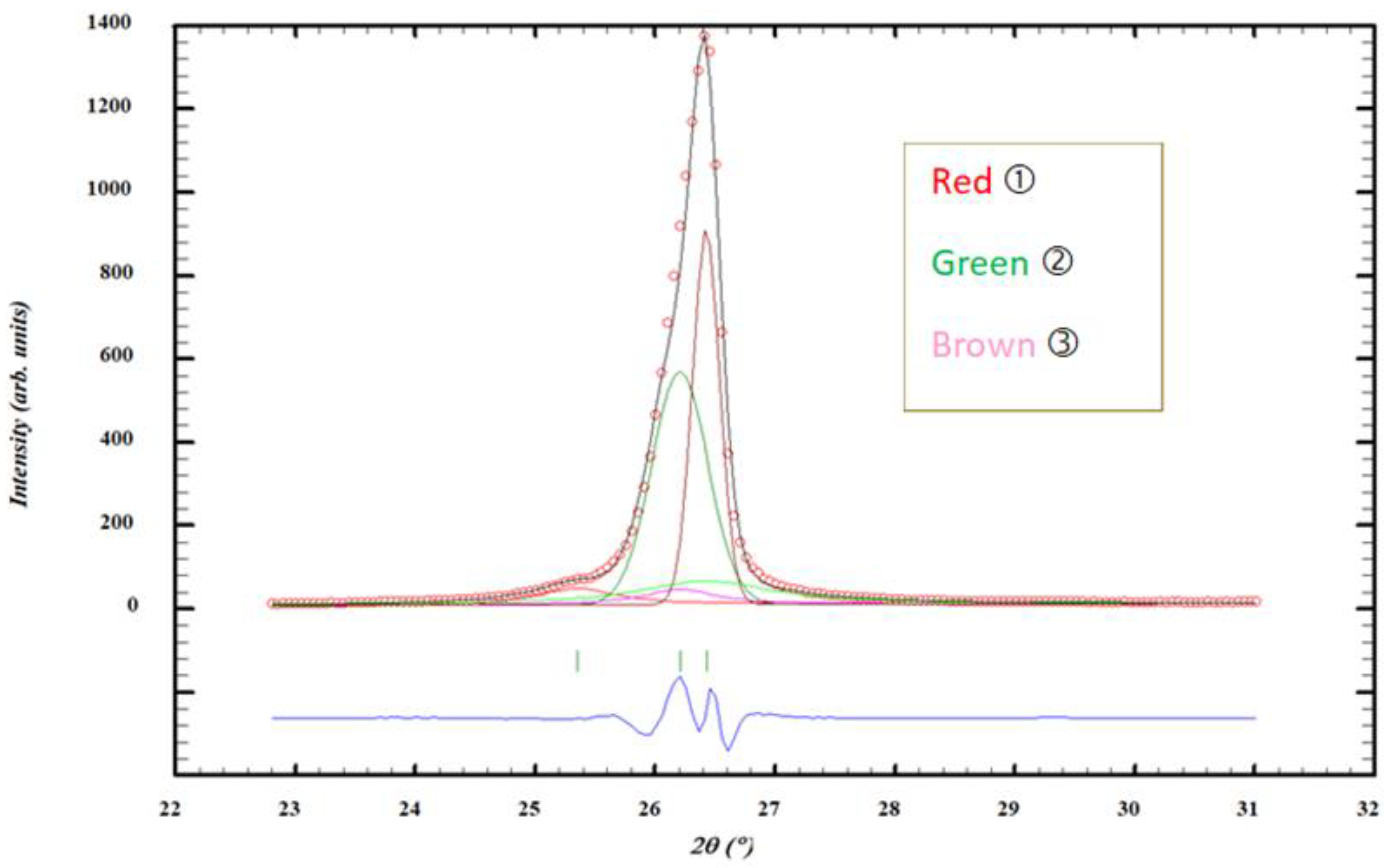
Figure 2. SEM images of the nanoscrolls already published [1]. Replaced by the second SEM and the images collected with an optical microscope (x 25000, scale barre 2 μm).

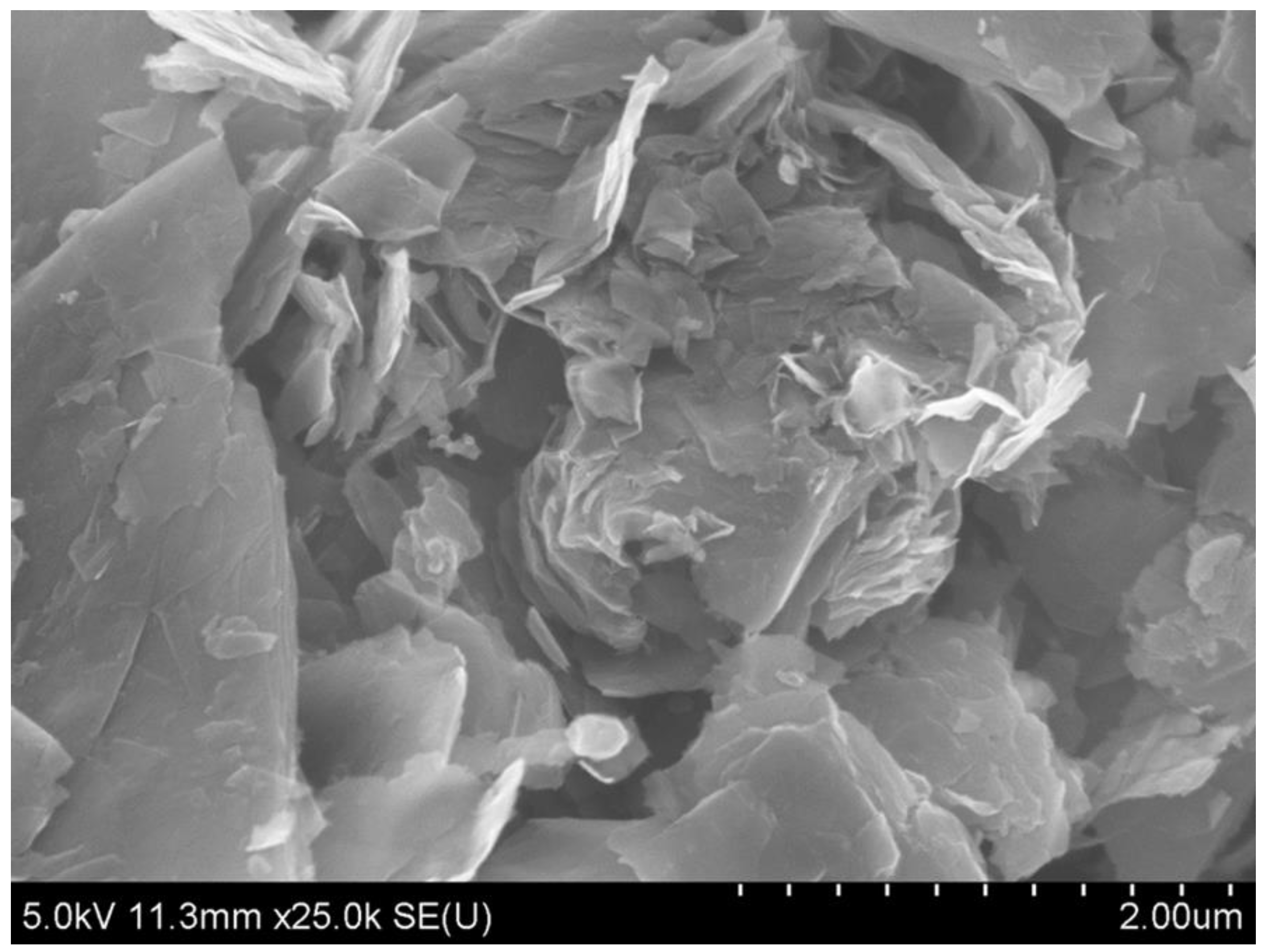
Figure 3. Graphene sheets inside a Cu/graphene sample after 2 h of ultrasounds – mixture of graphene with several thicknesses, flats. From 2 to 20 layers, their sizes can be larger than 20 nm. (x60000, scaling barre 50 nm).

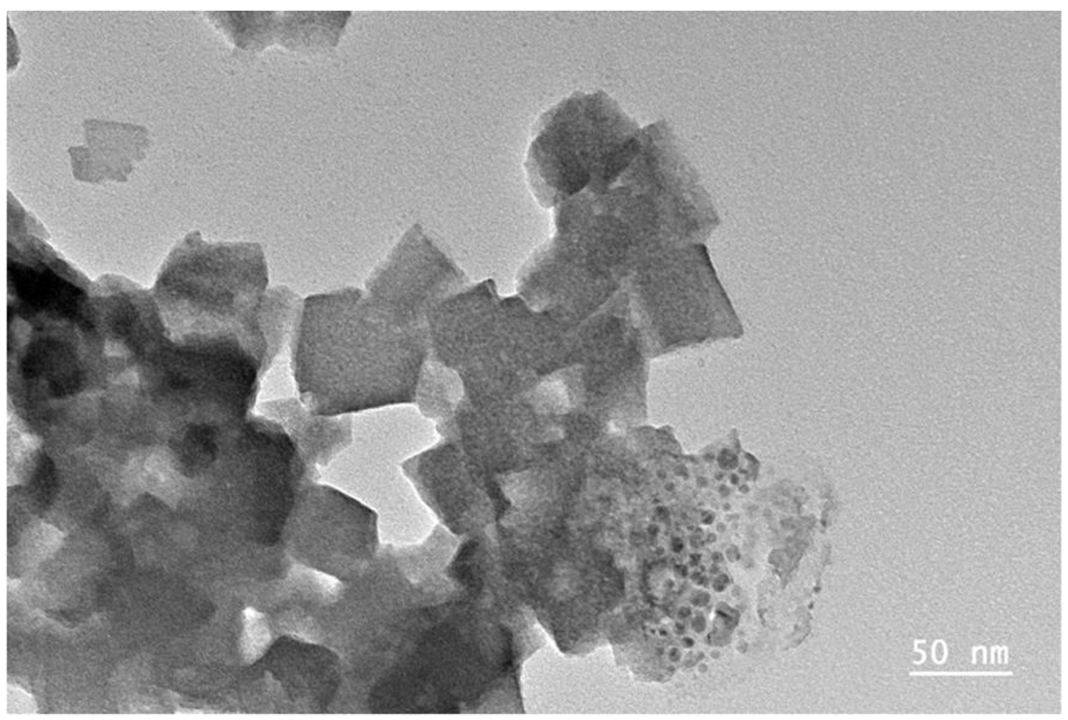
Figure 4. Selected area electron diffraction (a) SAED on a graphene particle and (b) TEM micrograph on a sample prepared with 2 hours of ultrasounds.

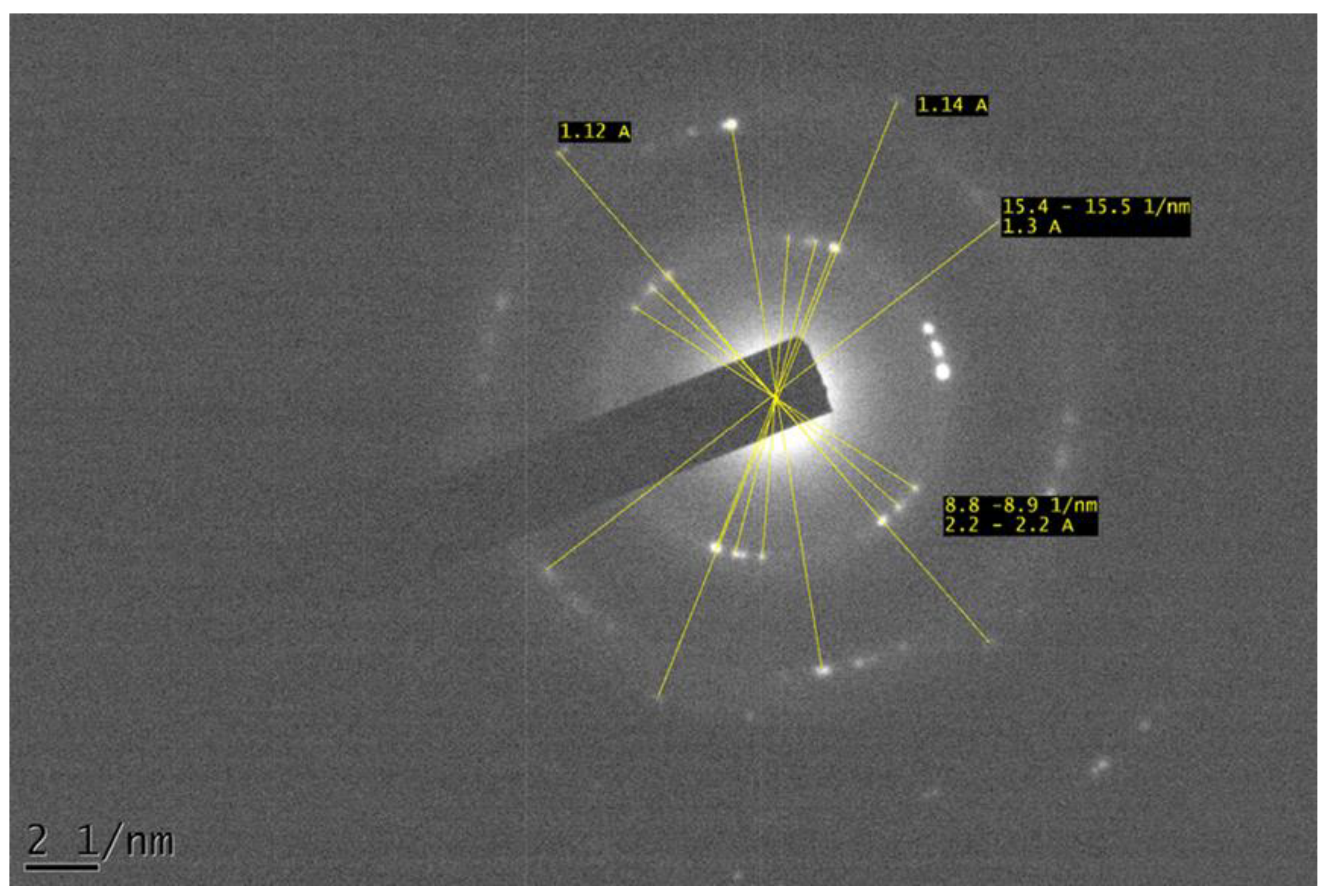
Figure 5. Details about copper oxide nanoparticles, external and covered by carbon layers. FFT made on external oxide particles (x500000, scaling barre 10 nm).

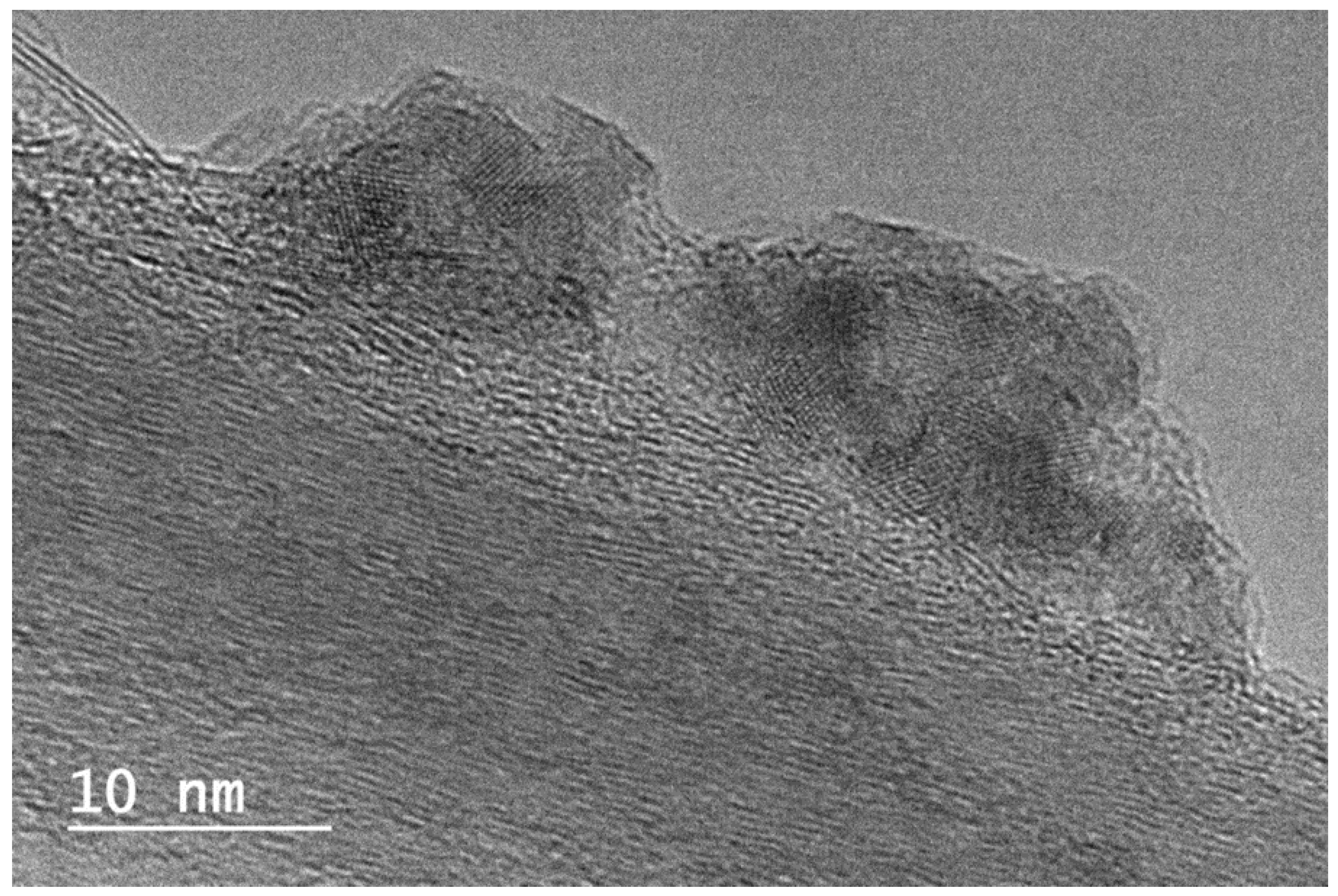
Figure 6. UV visible results, absorbance collected on dispersed graphene diluted in absolute ethanol: 1000, 750 and 500 μl diluted inside 3.00, 3.25 and 3.50 ml (cm³) of ethanol to obtain a total volume of 4 ml, studied in a one cm cell (in quartz) after ultrasounds 6 min, with and without pulses of 15s and stops of 15s and centrifugation at 5000 rpm 12 min.

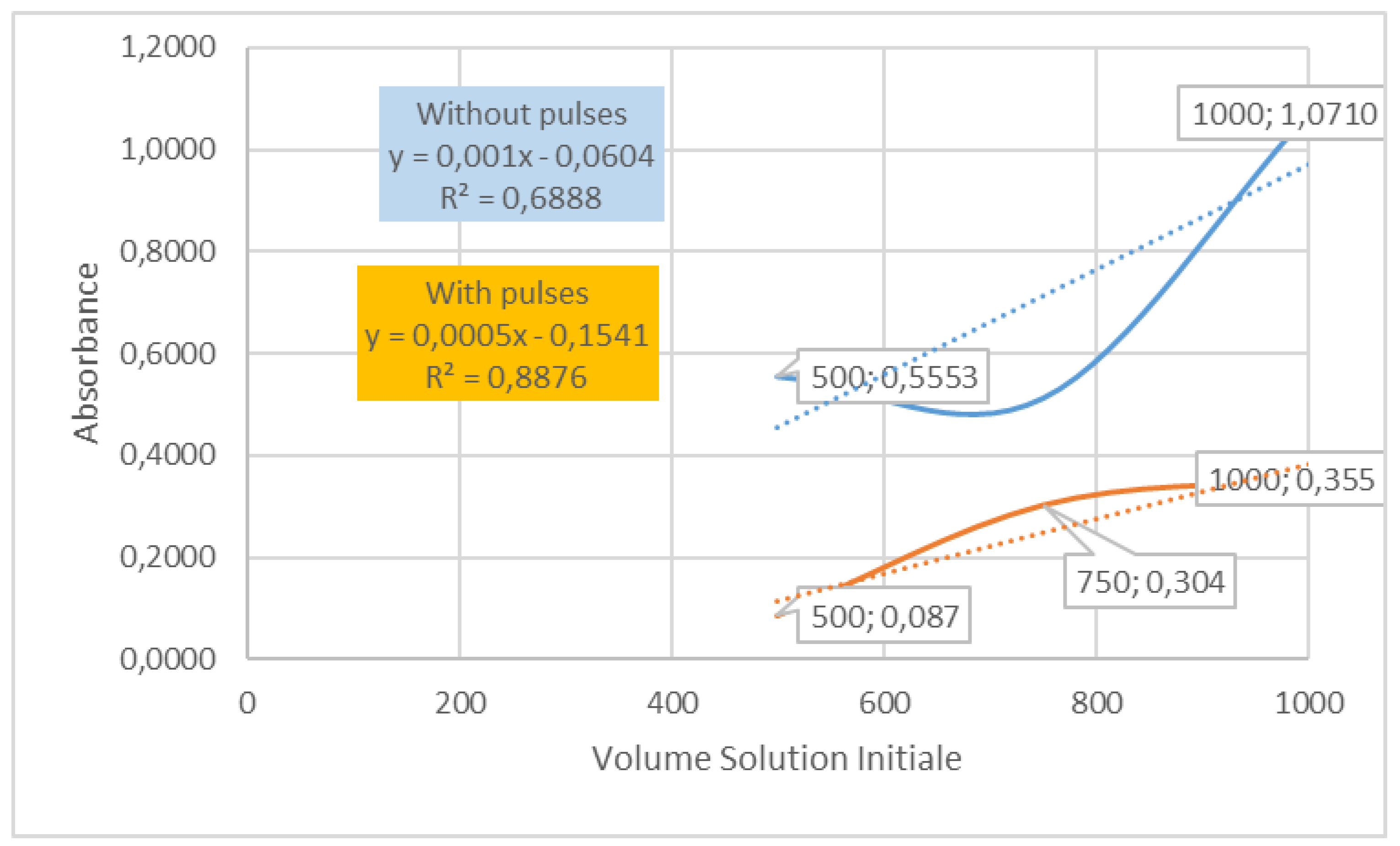
Figure 7. Absorbance measured as a function of the composition of the studied solution expressed in μg by ml.

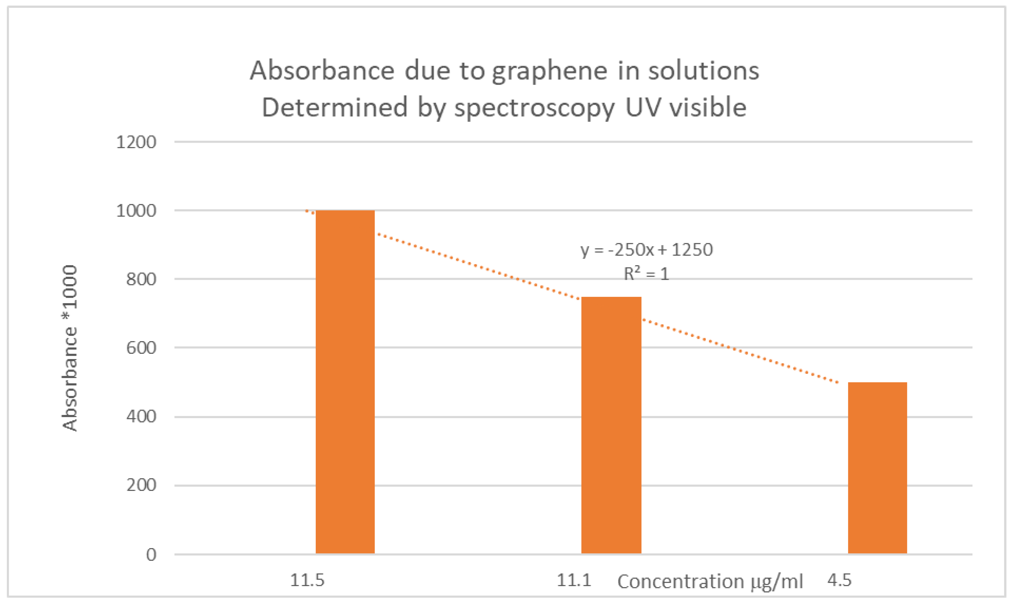
Figure 8. Influence of dilution by ethanol on UV visible spectra of “green” liquors of Cu/Graphene/Ethanol:.

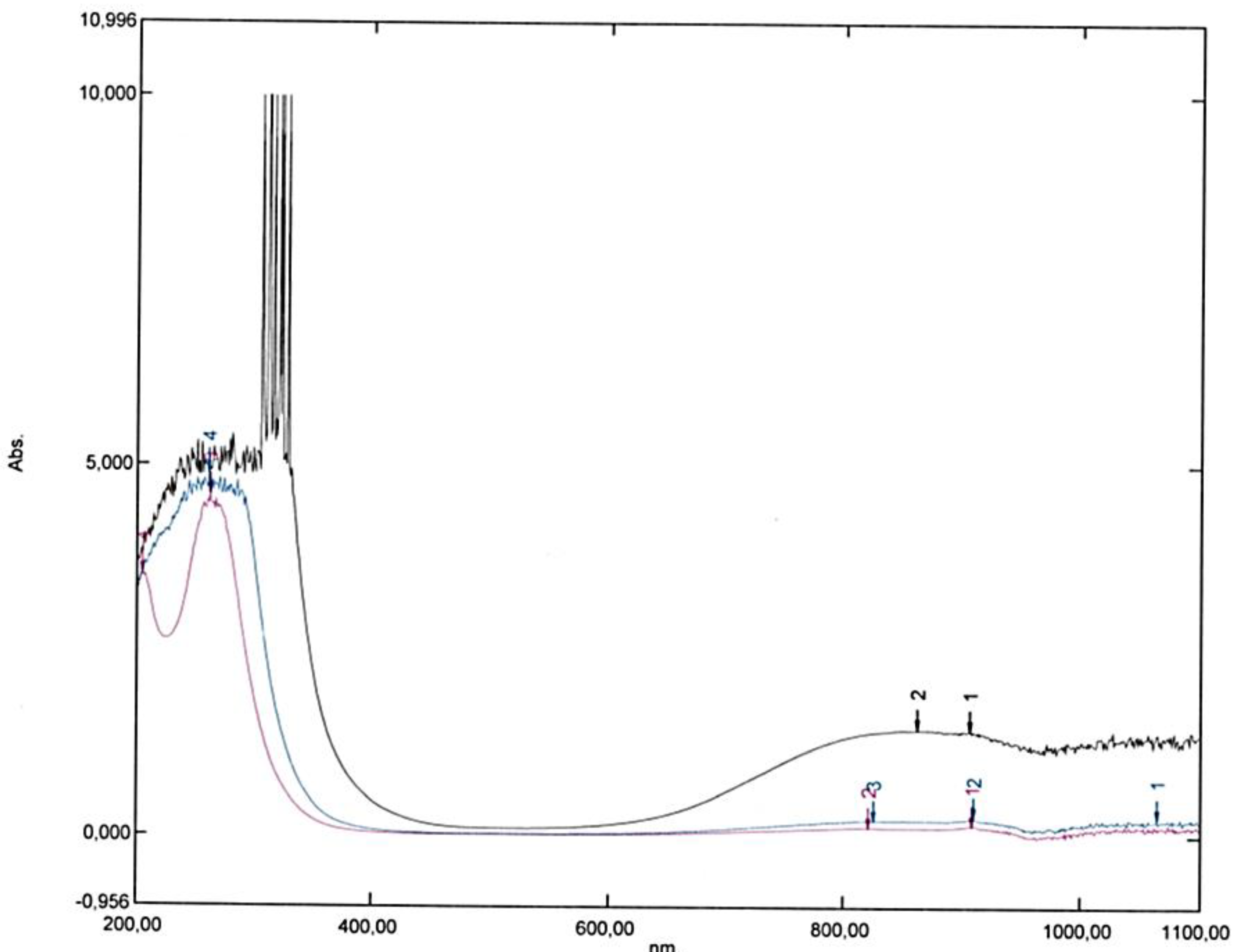
Figure 9. Influence of the optical path of UV visible cells on plasmons coupling with the others vibrations: C-C vibrations on the left (from above to below 400 nm) and [Cu Ethanol₂(H₂O)₄]²⁺ complex (864 nm instead of 800 nm for the hexa-aqua complex), orange in a cell of 1 cm and blue in a cell of 0.2 cm (internal).

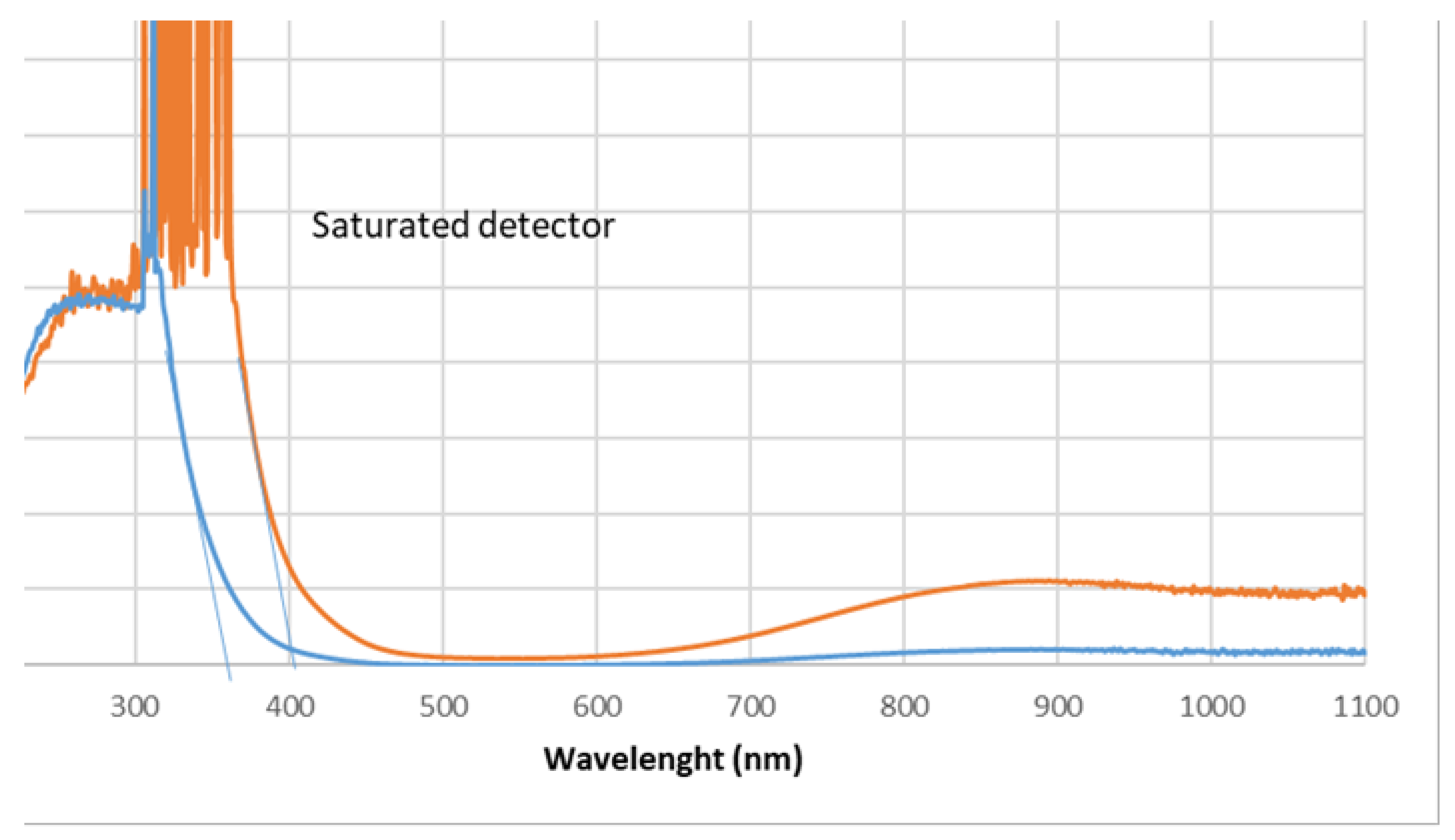
Figure 10. Associated TAUC plot for an indirect semi-conductor, obtained after 6 min of ultra-sounds treatment with pulses. The value of the band gap is calculated by the extrapolation of the straight line in orange, by dividing its origin (its common point with the Ox axis) by its slope. Here, a value of 3.67 eV is obtained.

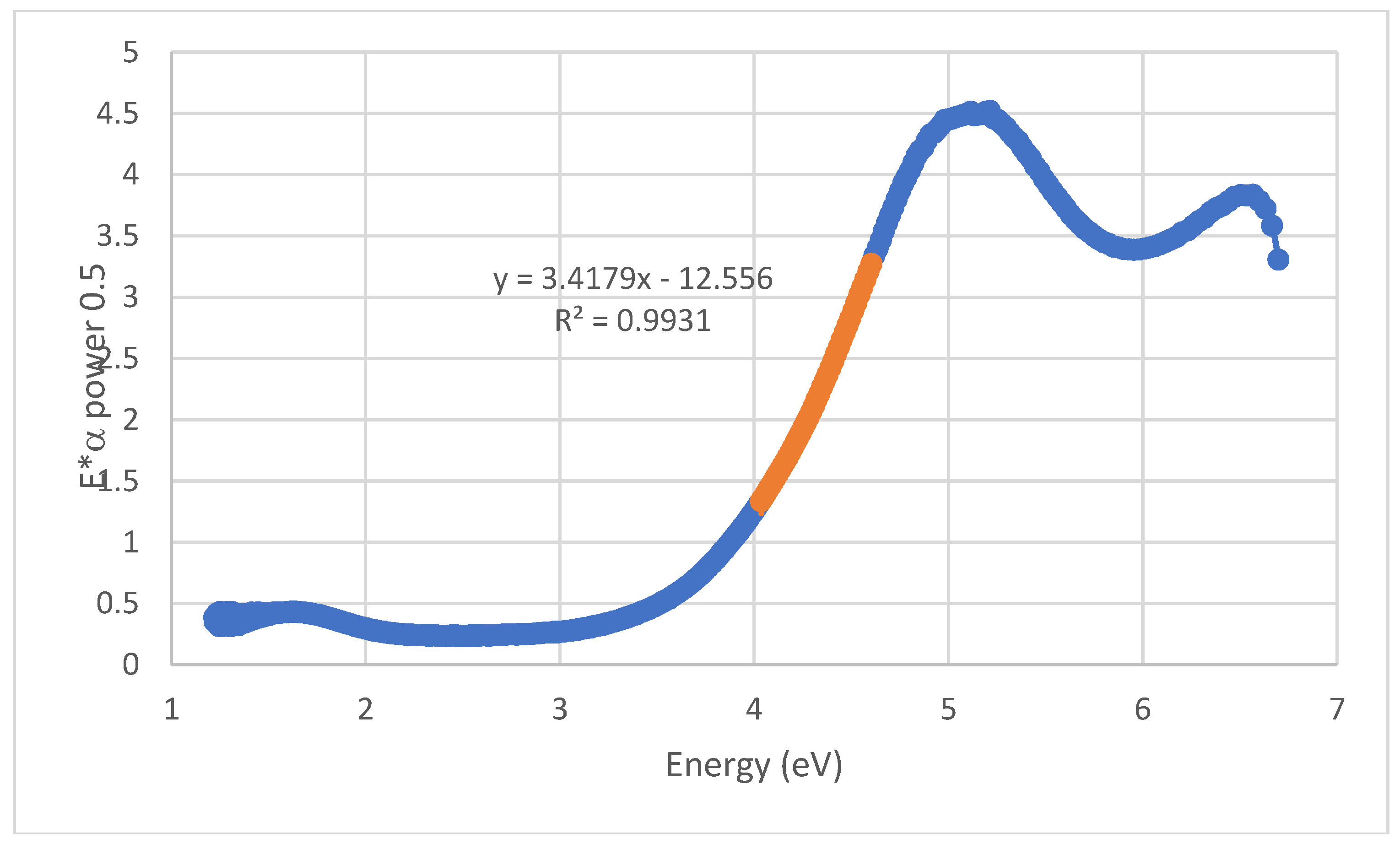
Figure 11. Fluorescence spectra of ethanol and of two solutions of graphene suspended in ethanol prepared respectively with 6 min and with 2h of the ultrasound treatment (excitation at 358 nm). No centrifugation.

Disclaimer/Publisher’s Note: The statements, opinions and data contained in all publications are solely those of the individual author(s) and contributor(s) and not of MDPI and/or the editor(s). MDPI and/or the editor(s) disclaim responsibility for any injury to people or property resulting from any ideas, methods, instructions or products referred to in the content.

© 2024 by the authors. Licensee MDPI, Basel, Switzerland. This article is an open access article distributed under the terms and conditions of the Creative Commons Attribution (CC BY) license (http://creativecommons.org/licenses/by/4.0/).

Copyright: This open access article is published under a Creative Commons CC BY 4.0 license, which permit the free download, distribution, and reuse, provided that the author and preprint are cited in any reuse.

Downloads

Views

Comments

Subscription

Notify me about updates to this article or when a peer-reviewed version is published.

MDPI Initiatives

Important Links

Choose an area of interest and we will send you notifications of new preprints at your preferred frequency.

Disclaimer