
Submitted:
30 May 2024
Posted:
30 May 2024
You are already at the latest version
Abstract
Surveys on the optimum seismic design of structures reveal that many investigations focus on how to minimize its initial cost while satisfying the performance constraints. Although reducing the initial cost while complying with the requirements of earthquake design codes of practice will significantly guarantee the life safety of occupants against earthquakes, it may still cause considerable economic losses to residents and fatalities. Accordingly, calculating the possible earthquake damages caused during the structure's lifetime may become essential from the optimal Life Cycle Cost (LCC) design point of view. LCC analysis is used to evaluate economic feasibility including construction, operation, occupancy, maintenance and end-of-life costs. For optimization, the population-based, meta-heuristic algorithm based on the Ideal Gas Molecular Movement (IGMM), has established its capability in solving highly nonlinear mono and multi-objective engineering problems. Therefore, this paper investigates the LCC -based mono and multi-objective optimum design of a 3-D four-story concrete building structure combined with the Endurance Time (ET) competence. The results show that, apart from substantially reducing the total number of analyses required, the proposed technique significantly affected dipping minor injury cost, rental, and income costs by 22%, 16%, and 16%, respectively. In total, a 10% reduction in all structural life-cycle costs was achieved, which could well be considered significant.
Keywords:
IGMM Algorithm
; Endurance Time Method
; Life-Cycle Cost Assessment (LCCA)
; Multi-Objective Optimization
; Reinforced Concrete Structures
; Performance-Based Design
1. Introduction
Despite significant advances in earthquake engineering in the last two decades, the seismic design codes are presently based on controlling the forces created in the structural components and displacements formed in two or more limit states for safety observation purposes. These codes do not consider the structural performance in its life-cycle in terms of cost and loss-of-life possibility; they are more based on setting some minimum values for the structure components' stiffness and strength and providing its overall safety [1,2,3]. Therefore, these codes have moved towards reliability-based designs and present criteria for the performance-based design as guidelines. In performance-based earthquake engineering (PBEE), the structural performance after its construction is studied to provide appropriate performance in its life cycle [4]. Accordingly, in such methods, more precise analyses with higher computations usually estimate the structure's nonlinear response under different intensity levels [5,6]. Performance-based design (PBD) starts with selecting design criteria articulated through one or more performance objectives. The first stage is how to choose the performance goals and develop an initial design accordingly. The structural design response will then be assessed and revised until the satisfactory criteria for all intended performance goals are met.
There are some performance-based optimum design (PBOD) algorithms used effectively to achieve optimal structural designs with acceptable performances, while their responses such as plastic hinge rotation and inter-story drifts are incorporated as constraints, and structural weight or cost is contemplated as the objective function [7]. Among many researchers, Liu et al. [8] applied a PBD method for multi-objective optimization using a genetic algorithm subject to uncertainties to provide a set of Pareto-optimal designs. Moreover, Pan et al. [9] combined multiple design constraints into a multi-objective method using a new formulation based on the constraint approach.
These studies deal with the minimum cost while meeting the minimum requirements set out in the design regulations and constraints. However, they may not necessarily lead to an economical design with the lowest total cost over the lifetime of the structure. This highlights the need to improve the design approach to reduce economic losses to an acceptable level while protecting human lives. To this end, the Life Cycle Cost (LCC) based design approach has been developed to address economic concerns directly in the design process.
In recent years, LCC Analysis (LCCA) has been considered by many researchers. It measures a structure's efficiency over its whole life cycle in terms of cost. It has engaged much attention from decision-makers looking for the most cost-effective approach for constructing buildings in seismic zones [10,11]. Wen and Kang [12] devised a long-term cost-benefit consideration for evaluating the expected life-cycle cost of an engineering system under multiple hazards in the early 2000s, as one of the motivating missions in this field. Later experiments were carried out to take advantage of the benefits of financial accounts in structural engineering. Takahashi et al. [13], using a renewal model for the occurrence of earthquakes in a seismic source, formulated the estimated life-cycle cost of construction alternatives. As a decision issue, a temporal relationship between characteristic earthquakes and the methodology was extended to an actual office building.
The LCC analysis requires calculating the cost components related to the structural performance under different seismic intensity levels [1,14]. It is necessary to use time-history methodologies and precise numerical models to estimate the structure's seismic performance with acceptable accuracy. However, the high computational effort required in these methods and the complications that prevailed, make the optimization algorithms difficult. Therefore, to estimate the structure response, earlier researchers have used simplified methods such as pushover analysis which is known for its limitations and weaknesses in estimating the acceleration of the stories and reduced precision and reliability of the results. The importance of considering the life cycle cost as an additional objective for the primary structural cost objective function in the field of multi-objective optimization has been investigated by Fragiadakis et al. [15]. They used pushover analysis to compare a single objective weight minimization with a performance-based two-objective design of a steel moment-resisting frame, yielding a basis for producing a Pareto front of the solutions.
To investigate the effectiveness of strengthening reinforced concrete buildings, Kappos and Dimitrakopoulos [16] used cost-benefit and LCCA as decision-making tools. By determining initial and damage cost components for each design, Mitropoulou et al. [1] studied the influence of the behavior factor in the final design of RC buildings under earthquake loading in terms of safety and economy. Also, they investigated multiple effects of the analysis method, the number of seismic records imposed, the performance criterion used, and the structural type on the LCC assessment of 3-D reinforced concrete structures. In addition, by using the Latin hypercube sampling method, they investigated the effect of uncertainties on the seismic response of structural systems and their impact on life-cycle cost assessments.
In recent years, the Endurance Time (ET) method, as a dynamic analysis approach that requires much less computational effort compared with other standard time-history methods, has been introduced and used in various cases [17,18,19,20].
Recently, Varaee et al. proposed an LCCA-based probabilistic optimization procedure for 3-D RC structures based on the FEMA-P-58 [21]. Their proposed method leads to the proper distribution of materials in the structures, and also it can reduce the life cycle costs without increasing the initial costs of construction.
Asadi and Hajirasouliha [22] developed a practical methodology for the optimum seismic design of RC frames to minimize damage and life-cycle cost based on uniform damage distribution (UDD). They demonstrate that the blind increase of the reinforcement ratio does not necessarily reduce the displacement demands and the damage costs. Mirfarhadi and Estekanchi [23,24] used value-based seismic design as a framework for optimal seismic design of structures considering a comprehensive set of performance indicators. In their work, design outcomes were compared to the conventional code-based design procedure minimizing the structural construction cost in terms of seismic response and consequences. Sarcheshmehpour et al. [14] proposed a practical framework for the optimal seismic design of high-rise steel buildings in compliance with all the constraints in the design regulations. This framework was used to compare the seismic behavior of pipe-to-pipe and frame pipe systems in conventional 20 and 40-story 3-D buildings.
Recently, the IGMM algorithm has been used as a population-based technique based on ideal gas molecular motion, with high convergence speed and acceptable accuracy in providing a general optimal solution utilizing a relatively small number of analyses [21,25,26,27]. Therefore, the present research makes simultaneous use of the ET method and IGMM algorithm to let the seismic loss reduction criteria enter the trend of the optimum design directly. The proposed method here can help present more all-inclusive definitions of such effects as seismic damage, damage to the contents of the structure, downtime costs, and costs due to injuries and fatalities in the form of quantitative parameters.
It can be expected that the intended structure may have an acceptable performance during and after an earthquake.
The optimization process of a 3-D four-story concrete structure is carried out in multiple steps to reduce the problem solution time. First, each response vector generated by the IGMM algorithm is controlled for the initial constraints, including the observance of the continuity of the sections' height and steel bar ratio for beams and columns. If the initial constraints are satisfied, linear analysis is allowed for the static loads. If the sections are found to respond well, a nonlinear analysis will be allowed then, and the optimization process will be continued until global convergence occurs.
The rest of the paper is organized as follows: In Section 2, the mono and multi-objective types of the IGMM algorithm are briefly described. Section 3 explains the ET method as a dynamic time-history analysis. Section 4 describes the methodology used for the LCCA design based on the ET method. In Section 5, the mathematical modelling of the optimization problem is introduced. Finally, the mono and multi-objective optimization of a 3-D four-story RC building is conducted, presenting and discussing results..
2. Optimization Algorithm
2.1. Mono-Objective IGMM-Based Algorithm
Ideal gas molecules in an isolated environment, due to the two latent factors of high velocity of ideal gas molecules and their high probability of collision, quickly disperse in different directions and cover the entire confined space.
Recently, the IGMM algorithm has been introduced as a meta-heuristic optimization method and its application in solving numerical and engineering optimization problems has been evaluated [28,29]. It uses the equations governing the elastic collision and speed equation of ideal gas molecules to determine the new position of the gas molecules in each iteration. Different steps of the IGMM algorithm for mono-objective optimization problems may be found in [30]. Figure 1 shows the flowchart of the IGMM algorithm.
2.2. IGMM-Based Multi-Objective Optimization
Multi-objective optimization problems commonly contain terms in conflict with each other. One procedure combines all the objectives into a single one and attempts to solve the problem using conventional mono-objective optimization algorithms [29-30]. Generating a Pareto optimal front is another way [31-33], where the solution is a set of Pareto optimal solutions, referred to as non-dominated optimum points. This set represents the best trade-offs between the objectives [34,35].
By extending the basic ideas of IGMM, the aim is to develop a type of Multi-Objective IGMM-based algorithm noted as MO-IGMM, to be described later. First, an archive of non-dominated designs is gradually built and equipped to reach a predefined size finally. It allows its members to renovate through the optimization procedure and build upon the number of its associates until a maximum diverse size is reached. It then replaces its members with more enhanced and uniformly distributed solutions. The probability of collision of each molecule from the current set in the population is calculated. In the event of a collision, the stationary molecule is selected from the low-density region of the archive molecules. Then the new velocity and position of the selected molecule will be calculated based on the elastic collision equations. Finally, it approximates the true Pareto optimal front as closely as possible. The following is how archive molecules are used, updated, and selected during the optimization process to ensure consistent distribution of its members.
A stationary molecule is selected from the least populated area of the determined Pareto front to achieve a uniform Pareto optimal front. In order to find the least populated area, the search space is divided into segments. For this purpose, the best and worst objectives of Pareto optimal solutions are found at each iteration, and a hyper-cube is built to cover all the solutions. It is then divided into equal sub-hyper-cubes, and a selection operand is carried out based on the Coello et al. suggestion by a Roulette-wheel mechanism with the following probability for each segment [21,36]:
where c is a constant value greater than one [37, 38] and is the number of found Pareto optimal solutions in the i-th segment. Based on this equation, stationary molecules have a greater chance of being selected from the less populated segments. Moreover, this can allow molecules to migrate around regions faster, improving the Pareto optimal front's distribution.
The archive should be updated in each iteration where it may primarily turn into complete. However, it allowed converting into more enhanced non-dominated solutions during optimization. Therefore, there should be a system to handle the archive. It should be prohibited from entering the archive if a solution is dominated by at least one of the archive members. Suppose a solution dominates any of the Pareto optimal solutions in the archive. In that case, all of them should be deleted from the archive and replaced with the only accepted non-dominated solution. If the archive is complete, one or more solutions may be deleted from the most populated segments to make room for a new solution(s) [21,36]. The ability to assess new points adjacent to their current position is given to enhance the MO-IGMM’s local search. This mechanism is only activated for molecules that are not involved in the collision to avoid unnecessary function evaluations. A detailed explanation on the procedure of MO-IGMM algorithm may be found in [36].
3. Endurance Time Method
As a response history analysis, the Endurance Time (ET) method can measure the structural responses such as maximum displacements, inter-story drift ratios, and stresses in time steps while the intensity of the applied accelerograms is increasing. Excitation in these artificial acceleration functions begins at a low intensity and steadily increases until structural failure occurs. Moreover, this allows structural responses to be tracked through a wide range of intensities. [4]. The ET method does, in fact, link analysis time to excitation intensity. The concept of acceleration reaction spectrum is helpful in ET for characterizing excitation intensity. ET excitation functions (ETEFs) are optimized while each time window, from zero to a particular time, generates a response spectrum that fits a template spectrum with a varying scale factor. [39]. Many studies have shown that the currently available ETEFs provide accurate structural response estimates at various excitation intensities with minimal computational effort [19,40]. Various ET acceleration functions are now freely accessible on the ET method's website [41]. In this investigation, “ETA40h” series acceleration functions are utilized as the basic accelerogram. The template spectrum of this series is the average response spectrum of seven ground motions recorded on soil type C. These motions are selected from a set of 20 earthquake records listed in FEMA440 [42]. According to Estekanchi et al., three acceleration functions in this series, which have different starting points for optimization, can reduce the random scatter effects in the results [17].
In the ET method, the value of the required engineering demand parameter (EDP) (e.g., drift for each story) is found over time. Then, the maximum absolute value of the EDP in the time interval [0,t] is plotted against the analysis time t. The x-coordinate axis of an ET curve is analysis time, but it is not common and, occasionally, can be confusing to evaluate and express seismic performance with time. Therefore, substituting a standard parameter such as peak ground acceleration (PGA) or return period for a time in the evaluation and expression of the performance of the structures is essential. A correlation between ET analysis time and the stated standard parameter should be determined [43]. In this research, the problem of correlation between time and the PGA has been used
4. Design Based on the Life-Cycle Cost
To optimally design the desired structure based on the life-cycle cost, the sum of the initial construction cost and those caused by probable earthquakes during the structure's useful period for a lifetime is considered as the total life-cycle cost.
We will show that the ET analysis provides a useful tool for performing acceptable-volume economic calculations on different design alternatives. The initial construction cost and the expected earthquake loss during the structure lifetime are usually two essential parameters for making decisions [1]. A severe obstacle in evaluating the cost of the earthquake loss is to estimate the structure response against the ground motion under different intensity levels. Different researchers have proposed different simplified seismic analysis methods to overcome the immense computational effort required to evaluate a large number of different designs. However, the cost evaluation has been used so far for comparative studies among a limited number of design alternatives. Researchers have only recently considered the direct use of the life-cycle cost in the design process [1,44]. The total life-cycle cost of the structure C_LC can be written as the sum of the initial cost C_IN, which is a function of the design vector s and the present value of the lifetime cost C_L which is a function of the structure lifetime t and the design vector s as in Eq. (2) [1]. The details of which will be explained next.
4.1. LCC Calculations Based on the ET Approach
The Life-Cycle Cost (LCC) assessment in the optimization process steps through the results found from the ET analysis requires a specific procedure, the steps of which are as follows:
Step 1. In this step, the history of the engineering demand parameters, including the maximum inter-story drift and acceleration of the stories over time, are found through the ET analysis, presented in the form of an ET response curve, and smoothed by fitting a curve on it. Figure 2(a). shows the ET response curve related to the history of the maximum inter-story drift for an assumed structure. It is worth mentioning that before drawing Figure 2(a), the amounts of the responses are extracted for all the stories, and their maximum absolute values are determined.
This process is carried out for all the required demand parameters, including the maximum drift in the Y direction and the maximum acceleration in different directions.
Step 2. In this step, mapping time (in the ET curve) to PGA is done based on the procedure explained in [38] and the curve of PGA versus time is drawn based on the fundamental period of the structure being studied (Figure 2(b)).
Step 3. Here, the curve of the response values (e.g., the maximum drift) versus PGA is drawn, which will result in the elimination of the time factor from the relations, and PGA is substituted (Figure 2(c)).
Step 4. In this step, the hazard curve of the region of the structure under investigation (LA in this research) is drawn based on the information obtained from the USGS Site [45]. Figure 2(d) shows the relation between PGA and Annual Frequency Exceedance (AFE).
Step 5. Here, the relation between the structure response (maximum inter-story drift) and the AFE is created, and the PGA is omitted from the relations (Figure 2(e)).
Step 6. In this step, the damage model is made, and the relation between the damage and the AFE is drawn. This step is for different damage components, including the costs of repairs, losing contents due to inter-story drift, losing contents due to the acceleration of stories, losing rents, losing incomes, cost of injuries, and cost of fatalities, and different damage components are found based on the explanations presented at the beginning of this chapter. Figure 2(f) shows the loss curve of the repair costs due to the drift in direction X.
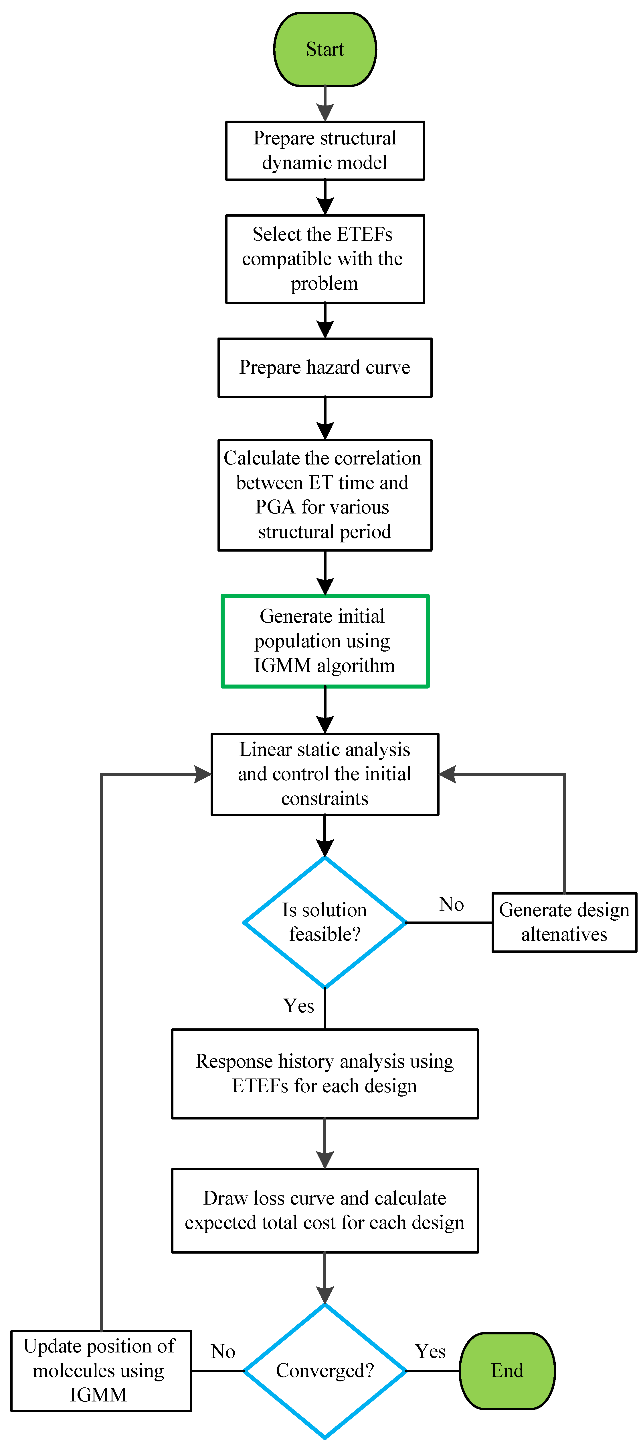
The above process is repeated many times in different optimization steps until the algorithm convergence conditions are satisfied and the optimum solution is achieved. As mentioned before, step 4 depends on the region of the structure and does not necessarily be repeated in each iteration. Figure A.1 given in Appendix A shows the flowchart of the optimization cycle.
Next, the optimization process is carried out once single-objectively using the IGMM algorithm and bi-objectively using the MOIGMM algorithm.
4.2. Initial Cost
The initial cost is usually the cost of constructing a new structure or retrofitting an existing one. In the design example of a new 3-D moment frame RC structure being investigated, the initial cost is related to the costs of land, building materials, and the labor force needed to construct the structure. Since the costs of land and other non-structural elements are the same for all the design alternatives, they can be omitted from the total cost calculations. Therefore, the initial cost can be calculated based on Eq. (3), taking into account the reinforcement steel, concrete, and framework costs.
where , , and are the unit costs of concrete, steel reinforcement, and formwork, respectively, with the corresponding values of respectively 735 $/m3, 7.1 $/kg, and 54 $/m2 [46]. is the section area of the steel reinforcement (for beams, it is equal to the sum of the section areas of the upper and lower bars), , , and are the member section dimensions, breadth, height, and length, respectively.
4.3. Useful Period of the Lifetime Cost
This part includes the structural costs sustained during the useful period of its lifetime. These costs are generally all-inclusive and include losses due to natural and unnatural disasters. However, in the present research, only the seismic losses caused by earthquakes have been considered lifetime costs. According to the existing technical literature, different limit states have been used considering the inter-story drift and the acceleration of the stories. These limit states (and the resulting loss) are due to the performance of the structural and non-structural elements.
The lifetime costs of a structure during its useful period may be due to many factors including natural and unnatural disasters such as seismic hazards. They may be characterized as the loss of contents itemized by the maximum inter-story drift and the floor acceleration, the damage repair cost, loss of rental cost, income cost, the cost of injuries, and the cost of human fatalities [1,12,47]. As for an economic assessment of these losses, a correlation is used according to limit states suggested by Ghobarah [48] for maximum inter-story drift ratios and a work by Elenas and Meskouris [49] for the maximum floor accelerations, shown in Table A.1, recorded in Appendix A. In general, the maximum inter-story drift ratio (∆) is used to calculate both structural and non-structural damages, and maximum floor acceleration () is used to justify the loss of contents [47]. In order to create a continuous relationship between the damage states and costs, a piecewise linear relation is assumed. As mentioned earlier, the lifetime cost of the structure is a combination of different components. The limit state cost (), for the i-th limit state, may be characterized as follows:
where is the damage repair cost; is the loss of contents cost due to the interstory-drift; indicates the loss of contents cost due to the acceleration in each floor; is the loss of rental cost; signifies the cost of income loss; is the injuries cost and indicates the cost of human fatalities. Formulae to calculate each cost component are shown in Table A.2, noted in Appendix A. The values of the mean damage index, loss of function, downtime, expected minor injury rate, expected serious injury rate, and expected death rate used in this study are based on ATC-13 [50] restated in FEMA-227 [51]. Table A.3 given in Appendix A provides corresponding parameters for each damage state. The method, with no limitation, has the capability of incorporating detailed calculations on cost components. The expected LCC of the building is computed by summing up the present values of the annual damage costs throughout the lifetime. For convenience, the detailed procedure to calculate for the structure, using ET method, is depicted in Figure 3.
If the useful structural lifetime period is assumed 50 years, Eq. (5) can be used, in the present time, to estimate the loss cost to different structural components along its useful lifetime period.
where is the cost of the i-th damage component during the useful structural lifetime period t and ϑ is the annual discount rate (3% in this research [4]). The structure's lifetime cost due to damage will be calculated by adding the computed present cost for each damage component. According to Eq. (2), the total life-cycle cost is equal to the total initial construction cost and the present annual cost of a useful structural lifetime period.
5. Numerical Example
5.1. Structural Model
In this research, a numerical structural model has been used, considering nonlinear material properties and deterioration. The structural analyses were carried out using the Performance-Based Earthquake Engineering (PBEE) toolbox [52]. The Euro code 8 [53] specifications together with the works by Fajfar and Eeri [54] and Perus et al. [55] were employed to define moment-rotation relations of the plastic hinges.
Some assumptions used in the nonlinear modeling process are as follows:
- –
- the floor diaphragms are assumed to be rigid in their planes, and the masses and the moments of inertia are lumped at the center of gravity.
- –
- The elastic elements connect all joints at the story level to the center of mass. They are used to model the rigid diaphragm at the story level, where the mass can be represented in one point. Columns contain the P-delta effect.
- –
- One-component lumped plasticity elements, consisting of an elastic beam and two inelastic rotational hinges (defined by the moment–rotation relationship), are used to model beam and column flexural behaviors. The element's formulation is based on the concept of a point of inflection at the element's midpoint. The plastic hinge is only used for the main axis bending in beams. For columns, two independent plastic hinges for bending about the two principal axes are used [56].
- –
- In the present study, the elastic beam-column elements and zero-length-section elements are used to create the model. At each elevation, “rigid” elements linked all of the nodes. The TakedaDAsym uniaxial material, designed in the software OpenSees, is used for plastic hinges in beams and columns [52].
- –
- A bi-linear or tri-linear relationship is used to model the moment-rotation relationship. When determining the moment-rotation relationship for beams or columns, zero axial force and axial strain due to gravity loads are considered, respectively. After the maximum moment, a linear negative post-capping stiffness is assumed.
- –
- The gravity load was modeled on beams as a uniformly distributed load and on columns as point loads. The self-weight of the slab and beams and the permanent load on the slab result in an evenly distributed load on the beams. Only the self-weight of columns is modeled using the point loads at the top of the columns.
- –
- The structure can be subjected to earthquake excitations in X and/or in the Y direction. The Newmark integrator is used assuming γ=0.5 and β=0.25.
5.2. Defining the Optimization Problem
In single-objective optimization, the minimization of the total cost is considered as the objective function. Accordingly, it is required that the design alternatives satisfy certain initial constraints. Columns' strengths have a reducing trend in the building height, meaning that the dimensions of the upper columns should be equal to or smaller than those of the lower ones. Besides these constraints, all the other code-based constraints regarding the gravity loads should be satisfied too. After these are satisfied for a design alternative, the LCC analysis is done based on the ET analysis (explained in subsection 4.1). To achieve the optimum design, this algorithm generates new designs based on the initial population until the convergence criterion is reached.
The design variables are the details of the beams and columns. In a general state, include the relative section areas of the lower and upper bars ( and , respectively), beam breadth and height (b and h, respectively), and stirrups’ relative section area and spacing ( and s, respectively) among which the latter two are assumed constant in the optimization process. Their values are found based on the seismic design specifications specified in the related codes. To simplify the execution of the final design, the beams section breadth at each story level is limited to that of the columns below, and only the beams section height is defined as a discrete variable in the range 30-60 cm with 5 cm paces. Also, the relative section area of the beam's lower bars is assumed half that of the upper bars (more than the minimum permissible value specified in the related codes). Therefore, the design variables in the optimization problem include only the beam section heights and section areas of the upper bars. Also, the relative section areas of the beam reinforcement bars are defined discretely considering arrangements of 2, 3, and 4 bars 16-25 mm in diameter.
The columns details, in a general state, include the relative section area of all the column reinforcement bars (), column section breadth and height (b and h, respectively), and stirrups’ relative section area and spacing ( and s, respectively). Similar to beams, the latter two are found based on the seismic design specifications specified in the related codes. To define the problem discretely and consider construction limitations, column section dimensions and numbers and diameters of the steel bars are shown in Table 1, from which the optimization algorithm chooses the required values. Column sections have been assumed squares with discrete dimensions that vary with 5 cm paces. The reinforcement bars have 8, 12, and 16 setting arrangements with appropriate clear spacing between the steel bars. In defining the sections, use has been made of 16, 18, 20, 22, and 25 mm diameter bars so that the column section bar ratio lies within the permissible range specified in the related codes.
The studied case is a 3D 4-story RC structure with two spans in each direction; in direction X, the span dimensions are both equal to 5 m, and in direction Y, they are 4 and 6 m. The height of the bottom story is 3.5 m, and the height of the other stories is 3.0 m. Twelve column types (6 for stories 1 and 2 and 6 for stories 3 and 4) and 28 beam types (3 for direction X and 4 for direction Y in all different stories) have been considered due to the existing symmetry in the structure. So, there are 72 design variables for the problem, including 12 for the column sections, 4 for the beam heights, and 56 for the beam's upper steel bars (one independent variable for each end of a beam). As mentioned before, these variables can assume only predefined values. Locations of each beam (B1-B7) or column (C1-C6) section on the plan are shown in Figure 4.
5.3. Mono-Objective Optimization
To achieve a design with the slightest variations in the initial cost, first, the structure was designed according to the ACI 318-14 [57] provisions and observing all the existing constraints. Secondly, the range of variations of every design variable in the optimization process was determined based on the life-cycle costs. Accordingly, the permissible values the design variables can assume are provided in Table 2. A non-stationary multi-stage assignment penalty function method is applied similar to that of [58,59,60] to handle constraints
In this example, the IGMM algorithm was able to find the optimum structure with an initial population of 20 after 20 cycles which is nearly 1200 time-history analyses (three analyses for each ET response curve based on the combinations of the three pairs of accelerograms).
Figure 5(a) compares the response curves of the maximum inter-story drift of the ET analysis of a structure designed based on the ACI318-14 and the optimum structure designed based on the life-cycle cost, and Figure 5(b) compares the smoothed curves of the drift versus PGA for both structures. In these curves, the drift values in lower accelerations (that have more occurrence probabilities) are less in the structure optimized based on the life-cycle cost than in the one designed based on codes.
Since drift values directly correlate with the structure damages and the related losses, this parameter can reduce the life-cycle cost.
Figure 5(c) shows the loss curve due to the drift in direction X of the two structures, one designed based on the ACI318-14 and the other optimized based on the life-cycle cost.
As shown in Figure5(c), the solid blue curve related to the latter shows smaller values. Although the difference may be negligible, considering that it shows the probable annual loss and the area under it is calculated and extended to a 50-year useful period of the lifetime, the slight reduction of this curve can considerably reduce the expected total loss.
As shown in Table 3, the initial cost has increased from 125004 $ in the design based on conventional codes to 126302 $ in the design based on the life-cycle cost. And, as shown in Table 4 the costs of the useful lifetime have reduced from 397192 $ in the code-based design to 345865 $ in the life-cycle cost-based design. Therefore, in general, only a 1% increase in the initial cost will result in a 13% reduction in the useful period of lifetime costs and a total 10% reduction in the total life-cycle cost of the structure being studied. Table 3, Table 4 and Table 5 present the comparative information regarding the details of the lifetime period and initial costs; the percent variation of each cost parameter due to optimization is also shown in each table. Comparative three first periods and mode shapes of the code-based and LCCA based optimum design are also provided in Table 6.
In Table 3, the initial cost of the structure has been recorded for the two cases of LCC-based optimal design and Traditional design. As mentioned in Section 4, the initial cost of the structural components includes the cost of reinforcement, concrete and formwork, which is shown in Table 3. The breakdown for structural components including beams and columns has been specified. Due to the reduction of column sections and the increase of beam sections in the optimal design, the initial costs related to columns for reinforcement, concrete and formwork are reduced by 4, 9 and 2 percent, respectively, whereas for beams there is an increase by 10, 2 and 2 percent, respectively. In total, LCC based optimal design will cause a cost increase by 1% compared to Traditional design.
The comparison of the life cycle costs of the structure can be seen in Table 4. The important point is the positive effect of LCC based optimal design in reducing life cycle costs compared to traditional design. The greatest impact on reducing the costs of the life cycle of the structure is on with 22%, followed by , and with 20, 16 and 16%, respectively. The comparison of the total initial costs and the life cycle costs of the structure for LCC based optimal design and traditional design in Table 5 shows that with only 1 percent increase in the initial costs for the structure, the life cycle costs of the structure can be reduced by 13 percent and with a reduced total life cycle costs of 10 percent. Thus, the cost of the entire life cycle of the structure shows a decrease from 5.22E+05 dollars to 4.71E+05 dollars.
5.4. Multi-Objective Optimization
The initial or total cost of a structure alone may not prepare comprehensive data on the structure's performance in a real-life design problem. Many contradictory and often inconsistent requirements should be considered concurrently to arrive at a rational design in practical decision-making issues. As a result, a consistent decision-making process necessitates detailed knowledge about design options from which a designer chooses the one that best balances conflicting goals. This knowledge can be better demonstrated in a Pareto front of design alternatives with optimized initial costs and life-cycle costs concurrently. The two most critical metrics for decision-making are generally the initial construction cost and the expected cost over the structure's lifetime Multi-objective optimization procedures can solve the optimization problem and achieve specific Pareto optimal designs. The multi-objective algorithm generates a collection of optimal designs for a wide range of alternatives. The key feature of the Pareto optimal set is that no change in one objective is possible without deterioration in other objectives.
The structure's initial cost and lifetime cost are the two different objectives in this multi-objective optimization problem. The discrete optimization problem is solved using the multi-objective ideal gas molecular movement (MOIGMM) algorithm. The algorithm's ability to solve multi-objective optimization problems in a computationally capable manner has been demonstrated by its use in engineering problems [36]. The initial cost and the expected lifetime cost of the structure are the first and second objectives, respectively, and thus, the optimization problem can be set as:
where s is the design vector, F is the feasible design space, and k is the number of constraint functions. There are totally 72 design variables for the problem, including 12 for the column sections, 4 for the beam heights, and 56 for the relative section areas of the beam's upper steel bars, one independent variable for each end of a beam. denotes the constraints that candidate design alternatives should meet. One of the constraints is that the selected sections for columns in each story cannot be weaker than those in the upper story. In addition, all code-based limitations imposed by ACI318-14 design recommendations must be met. Moreover, this means that according to prescriptive design requirements, all Pareto optimal designs would be acceptable. Inter-story drift ratio limits are also set at both operation and ultimate levels. These are controlled using a linear elastic analysis by OpenSees software [61]. Once the expressed constraints have been met, a nonlinear time-history analysis using the ET method is carried out. The expected lifetime cost due to future seismic hazards is measured using life-cycle cost assessment.
Now, each design variable’s variations interval is increased according to Table 7, and the MOIGMM algorithm is allowed to search a broader range to eventually yield a complete Pareto Front. After 25 cycles, with an initial population of 20, archive size of 25 and number of sub-cubes equal to 30, this algorithm performed the Pareto Front shown in Figure 6.
It is worth noting that each design on a Pareto Front that meets a vertical line with a specified distance from the origin (initial cost) is the one with the best performance possible to be built with its initial cost. For instance, Figure 6 shows the optimum design based on a mono-objective optimization and its related initial cost. It reveals that this design has the lowest total cost among those with similar initial costs. As expected, an increase in the range of variations of the design variables will yield points with lower total costs than the solution found in the mono-objective optimization. Besides, this figure can be studied as a guide for decision-making to see the reduction trend of the lifetime cost with an increase in the initial cost. This information can assist the decision-makers to choose a design that can create a relative balance between two objective functions. It also shows that in design alternatives with an initial cost of about 147000 $, a slight increase in the initial investment can considerably enhance the structure performance and reduce the future costs. It is worth mentioning that the problem space is discrete because the design variables are discrete, and this has created some discontinuities in the obtained Pareto Front. It is possible to consider the sum of the initial and lifetime costs as a criterion for choosing a point from among different Pareto Front points. This criterion is shown in Figure 6 by drawing the line . Points lying on this line are responses that will have the minimum total life-cycle cost.
6. Conclusions
The present work inspects the optimum seismic design of a life-cycle cost on a 3-D four-story concrete building structure. The implemented means of the research could perform a comprehensive definition of the seismic effects like structural losses, losses to the structural contents, downtime costs, and costs due to injuries and fatalities as quantitative parameters. Using this technique, one could expect the ensued structure to operate satisfactorily during and after the earthquake. Endurance Time method was employed to proceed with the nonlinear analysis and structural response prediction. It estimates the structural response under different seismic intensities with computation costs substantially lower than the conventional time-history methods. The utilized technique also prepares the means to employ stochastic algorithms for optimization. The mono and multi-objective optimization technique based on a new IGMM technique, recently proposed by the authors, was employed here. It is based on the ideal gas molecular movements and can converge to the global optimum at the early stages of the optimization process. Based on the customary codes of practice, having compared the currently found optimum structural response with those available in the literature, it signifies the approach for minimizing the lifetime costs of complicated structures. In the following, the main findings are summarized:
- –
- The mono-objective optimization procedure led to a 13% reduction of useful lifetime costs by merely increasing a 1% initial cost.
- –
- In total, a 10% reduction in all structural life-cycle costs was attained by mono-objective optimization.
- –
- The use of LCC-based optimization could cause a significant effect on reducing minor injury, rental, and income costs by 22%, 16%, and 16%, respectively.
- –
- Using multi-objective IGMM-based optimization resulted in performing a set of optimum responses for the 3-D four-story concrete building under the study that could assist engineering designers in making a decision to perform an optimum design.
- –
- As a result, the accessible methodology here, including the ET method as an analysis tool and IGMM algorithm as an optimizer, provides a numerical tool with a considerable computational saving for the quantitative estimation of the life-cycle cost and the vulnerability assessment of any real-scale reinforced concrete building.
Conflicts of Interest
The authors declare that they have no conflict of interest.
Replication of Results
All codes and models are generated using Matlab and OpenSees. The full datasets, as well as the developed codes, can be made available with a reasonable request to the corresponding author.
Appendix A

Table A1.
Inter-story drift ratio and maximum floor acceleration limits for different damage states.
Table A1.
Inter-story drift ratio and maximum floor acceleration limits for different damage states.
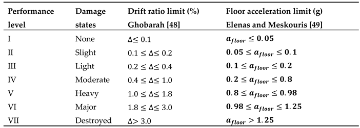
Table A2.
Formulas for cost calculation in monetary units (MU, corresponding to Dollars or Euros) [1].
Table A2.
Formulas for cost calculation in monetary units (MU, corresponding to Dollars or Euros) [1].
| Cost category | Calculation formula | Basic cost |
|---|---|---|
| ) | Replacement cost × floor area × mean damage index | |
| ) | Unit content cost × floor area × mean damage index | |
| ) | Rental rate × gross leasable area × loss of function | |
| ) | Rental rate × gross leasable area × down time | |
| ) | Minor injury cost per person × floor area × occupancy rate × expected minor injury rate | |
| ) | serious injury cost per person × floor area × occupancy rate × expected serious injury rate | |
| Human fatality cost per person × floor area × occupancy rate × expected death rate | ) |
* Occupancy rate 2
Table A3.
Damage state parameters for cost calculations [1].
Table A3.
Damage state parameters for cost calculations [1].
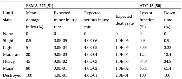
Figure A1.
Flowchart of the LCCA-based optimum design using IGMM and ET method.
References
- Mitropoulou CC, Lagaros ND, Papadrakakis M. Life-cycle cost assessment of optimally designed reinforced concrete buildings under seismic actions. Reliab Eng Syst Saf 2011;96:1311–31. [CrossRef]
- Varaee H, Safaeian Hamzehkolaei N, Safari M. A hybrid generalized reduced gradient-based particle swarm optimizer for constrained engineering optimization problems. J Soft Comput Civ Eng 2021;5:86–119. [CrossRef]
- Noori F, Varaee H. Nonlinear Seismic Response Approximation Of Steel Moment Frames Using Artificial Neural Networks. Jordan J Civ Eng 2022;16.
- Basim MC, Estekanchi HE. Application of endurance time method in performance-based optimum design of structures. Struct Saf 2015;56:52–67. [CrossRef]
- Kleingesinds S, Lavan O, Venanzi I. Life-cycle cost-based optimization of MTMDs for tall buildings under multiple hazards. Struct Infrastruct Eng 2021;17:921–40.
- Chen A, Ruan X, Frangopol DM, Tsompanakis Y. Life-cycle, reliability and sustainability of civil infrastructure. Struct Infrastruct Eng 2022:1–2.
- Ganzerli S, Pantelides CP, Reaveley LD. Performance-based design using structural optimization. Earthq Eng Struct Dyn 2000;29:1677–90. [CrossRef]
- Liu Z, Atamturktur S, Juang CH. Performance based robust design optimization of steel moment resisting frames. J Constr Steel Res 2013;89:165–74. [CrossRef]
- Pan P, Ohsaki M, Kinoshita T. Constraint approach to performance-based design of steel moment-resisting frames. Eng Struct 2007;29:186–94. [CrossRef]
- Basim MC, Estekanchi H. Application of Endurance Time Method in Value Based Seismic Design of Structures. Second Eur Conf Earthq Eng Seismol 2014;56:1–12.
- Salgado RA, Apul D, Guner S. Life cycle assessment of seismic retrofit alternatives for reinforced concrete frame buildings. J Build Eng 2020;28:101064.
- Wen Y-KK, Kang YJ. Minimum Building Life-Cycle Cost Design Criteria. I: Methodology. J Struct Eng 2001;127:330–7.
- Takahashi Y, Der Kiureghian A, Ang AHS. Life-cycle cost analysis based on a renewal model of earthquake occurrences. Earthq Eng Struct Dyn 2004;33:859–80. [CrossRef]
- Sarcheshmehpour M, Estekanchi HE. Life cycle cost optimization of earthquake-resistant steel framed tube tall buildings. Structures, vol. 30, Elsevier; 2021, p. 585–601.
- Fragiadakis M, Lagaros ND, Papadrakakis M. Performance-based multiobjective optimum design of steel structures considering life-cycle cost. Struct Multidiscip Optim 2006;32:1–11. [CrossRef]
- Kappos AJ, Dimitrakopoulos EG. Feasibility of pre-earthquake strengthening of buildings based on cost-benefit and life-cycle cost analysis, with the aid of fragility curves. Nat Hazards 2008;45:33–54. [CrossRef]
- Estekanchi HE, Valamanesh V, Vafai A. Application of endurance time method in linear seismic analysis. Eng Struct 2007;29:2551–62.
- Estekanchi HE, Riahi HT, Vafai A. Application of endurance time method in seismic assessment of steel frames. Eng Struct 2011;33:2535–46. [CrossRef]
- Hariri-ardebili M a. A, Sattar S, Estekanchi HEE. Performance-based seismic assessment of steel frames using endurance time analysis. Eng Struct 2014;69:216–34. [CrossRef]
- Mirzaee A, Estekanchi H, Vafai A. Application of Endurance Time Method in Performance-Based Design of Steel Moment Frames. Sci Iran 2010;17:482–92. [CrossRef]
- Varaee H, Shishegaran A, Ghasemi MR. The life-cycle cost analysis based on probabilistic optimization using a novel algorithm. J Build Eng 2021;43:103032. [CrossRef]
- Asadi P, Hajirasouliha I. A practical methodology for optimum seismic design of RC frames for minimum damage and life-cycle cost. Eng Struct 2020;202. [CrossRef]
- Mirfarhadi SA, Estekanchi HE. Value based seismic design of structures using performance assessment by the endurance time method. Struct Infrastruct Eng 2020;16:1397–415.
- Mirfarhadi SA, Estekanchi HE, Sarcheshmehpour M. On optimal proportions of structural member cross-sections to achieve best seismic performance using value based seismic design approach. Eng Struct 2021;231:111751.
- Ghasemi MR, Varaee H. Modified Ideal Gas Molecular Movement Algorithm Based on Quantum Behavior. Adv. Struct. Multidiscip. Optim., Cham: Springer International Publishing; 2018, p. 1997–2010. [CrossRef]
- Ghasemi MR, Varaee H. Damping vibration-based IGMM optimization algorithm: Fast and significant. Soft Comput 2019;23:451–81. [CrossRef]
- Shabakhty N, Enferadi MH, Ghasemi MR, Varaee H. Application of Shape Memory Alloy Tuned Mass Damper in Vibration Control of Jacket type Offshore Structures. Iran J Mar Sci Technol 2020;7:64–75.
- Ghasemi MR, Ghiasi R, Varaee H. Probability-based damage detection using kriging surrogates and enhanced ideal gas molecular movement algorithm. ICAVMS 2017 19th Int Conf Acoust Vib Mech Struct 2017;4.
- Varaee H, Ghasemi MR. An improved chaotic ideal gas molecular movement algorithm for engineering optimization problems. Expert Syst 2022;39:e12913. [CrossRef]
- Varaee H, Ghasemi MR. Engineering optimization based on ideal gas molecular movement algorithm. Eng Comput 2017;33:71–93. [CrossRef]
- Marler RT, Arora JS. Survey of multi-objective optimization methods for engineering. Struct Multidiscip Optim 2004;26:369–95.
- Yang X. Multiobjective Firefly Algorithm for Continuous Optimization. Eng Comput 2013;29:175–84.
- Mirjalili S, Lewis A. Novel performance metrics for robust multi-objective optimization algorithms. Swarm Evol Comput 2015;21:1–23.
- Coello CAC, Pulido GT, Lechuga MS. Handling multiple objectives with particle swarm optimization. Evol Comput IEEE Trans 2004;8:256–79.
- Mirjalili S. Dragonfly algorithm: A new meta-heuristic optimization technique for solving single-objective, discrete, and multi-objective problems. Neural Comput Appl 2016;27:1053–73. [CrossRef]
- Ghasemi MR, Varaee H. A fast multi-objective optimization using an efficient ideal gas molecular movement algorithm. Eng Comput 2017;33:477–96. [CrossRef]
- Coello CAC. Evolutionary multi-objective optimization: Some current research trends and topics that remain to be explored. Front Comput Sci China 2009;3:18–30.
- Coello CAC, Reyes-Sierra M. Multi-Objective Particle Swarm Optimizers: A Survey of the State-of-the-Art. Int J Comput Intell Res 2006;2:287–308. [CrossRef]
- Nozari A, Estekanchi HE. Optimization of Endurance Time acceleration functions for seismic assessment of structures. Int J Optim Civ Eng 2011;2:257–77.
- Mirzaee A, Estekanchi HE. Performance-based seismic retrofitting of steel frames by the endurance time method. Earthq Spectra 2015;31:383–402.
- Https://sites.google.com/site/etmethod/. Endurance Time Method n.d. https://sites.google.com/site/etmethod/.
- FEMA-440. Improvement of Nonlinear Static Seismic Analysis Procedures. FEMA 440, Fed Emerg Manag Agency, Washingt DC 2005.
- Mirzaee A, Estekanchi HEE, Vafai a. Improved methodology for endurance time analysis: From time to seismic hazard return period. Sci Iran 2012;19:1180–7. [CrossRef]
- Kaveh A, Laknejadi K, Alinejad B. Performance-based multi-objective optimization of large steel structures. Acta Mech 2012;223:355–69. [CrossRef]
- https://www.usgs.gov/. U.S. Geological Survey n.d. https://www.usgs.gov/.
- Camp C V, Huq F. CO 2 and cost optimization of reinforced concrete frames using a big bang-big crunch algorithm. Eng Struct 2013;48:363–72. [CrossRef]
- Mitropoulou CC, Lagaros ND, Papadrakakis M. Building design based on energy dissipation: A critical assessment. Bull Earthq Eng 2010;8:1375–96. [CrossRef]
- Ghobarah A. On drift limits associated with different damage levels. Proc Int Work Performance-Based Seism Des 2004.
- Elenas A, Meskouris K. Correlation study between seismic acceleration parameters and damage indices of structures. Eng Struct 2001;23:698–704. [CrossRef]
- Applied Technology Council. ATC-13: Earthquake damage evaluation data for california. 1985.
- FEMA-227. ABenefit-Cost Model for the Seismic Rehabilitation of Buildings. vol. 2. 1992.
- Dolsek M. Development of computing environment for the seismic performance assessment of reinforced concrete frames by using simplified nonlinear models. Bull Earthq Eng 2010;8:1309–29. [CrossRef]
- European Commitee for Standardization. Eurocode 8: Design of structures for earthquake resistance - Part 1 : General rules, seismic actions and rules for buildings. vol. 1. 2004. doi:[Authority: The European Union per Regulation 305/2011, Directive 98/34/EC, Directive 2004/18/EC].
- Fajfar P, Eeri M. A Nonlinear analysis method for performance based seismic design. Earthq Spectra, NICEE 2000;16:573–92. [CrossRef]
- Peruš I, Fajfar P, Dolšek M. Simplified nonlinear seismic assessment of structures using approximate Sdof-Ida curves. 14th World Conf. Earthq. Eng., Beijing, China: 2008.
- PBEE TOOLBOX - Examples of Application Version 1.0. Matjaž Dolšek 2008.
- American Concrete Institute. ACI 318-14: Building code requirements for structural concrete. 2014.
- Varaee H, Ahmadi-Nedushan B. Minimum cost design of concrete slabs using particle swarm optimization with time varying acceleration coefficients. World Appl Sci J 2011;13:2484–94.
- Ahmadi-Nedushan B, Varaee H. Optimal Design of Reinforced Concrete Retaining Walls using a Swarm Intelligence Technique. In: B.H.V. Topping and Y. Tsompanakis, editor. Proc. First Int. Conf. Soft Comput. Technol. Civil, Struct. Environ. Eng., vol. 92, Stirlingshire, Scotland: Civil-Comp Press; 2009, p. 1–12. [CrossRef]
- Hoseini Z, Varaee H, Rafieizonooz M, Jay Kim J-H. A New Enhanced Hybrid Grey Wolf Optimizer (GWO) combined with Elephant Herding Optimization (EHO) Algorithm for Engineering Optimization. J Soft Comput Civ Eng 2022;6:1–42.
- McKenna F. OpenSees: A framework for earthquake engineering simulation. Comput Sci Eng 2011;13:58–66.
Figure 1.
Flowchart of the IGMM algorithm.
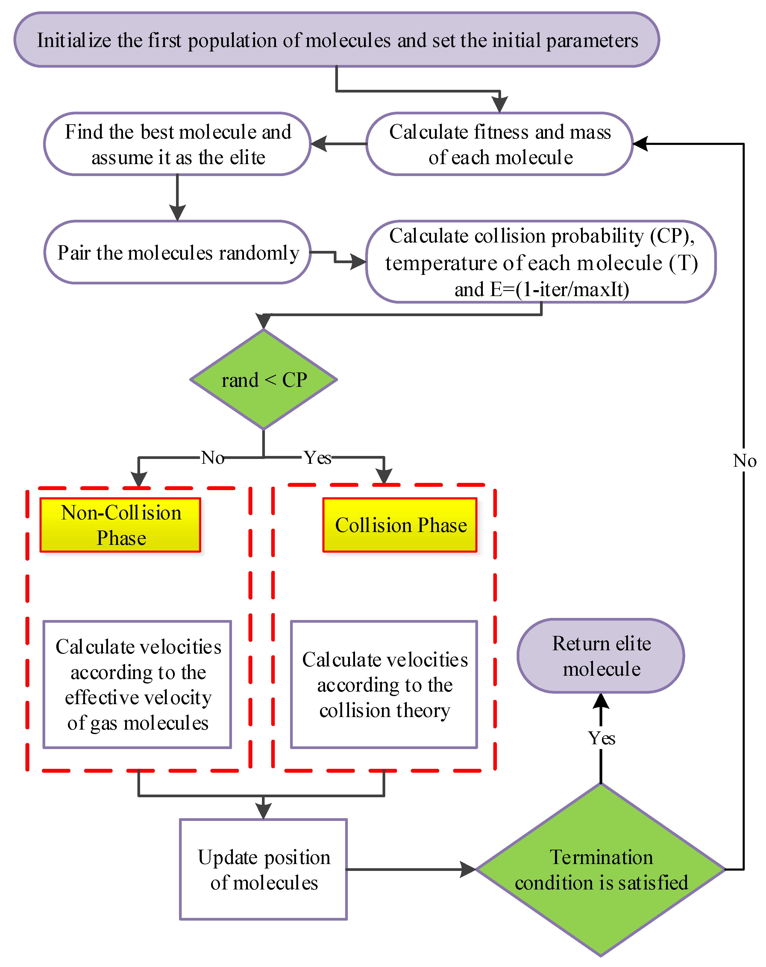
Figure 2.
(a) The response curve due to the ET analysis. (b) The Mapping relation of Time to PGA for a 0.84 Second Period. (c) Illustration of Drift variation against PGA. (d) LA Hazard Curve. (e) The relation between structural response and the annual Exceedance frequency (f) The loss curve of repair cost due to the drift in the X direction.
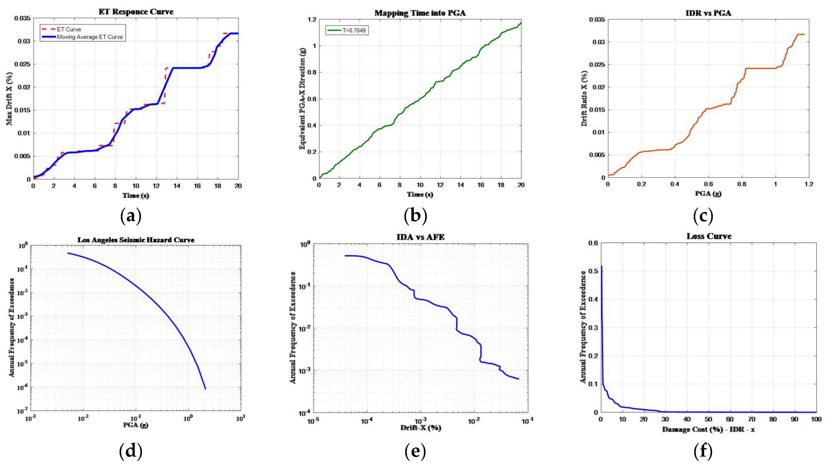
Figure 3.
The procedure of computing the life cycle cost of the structure using ET method.
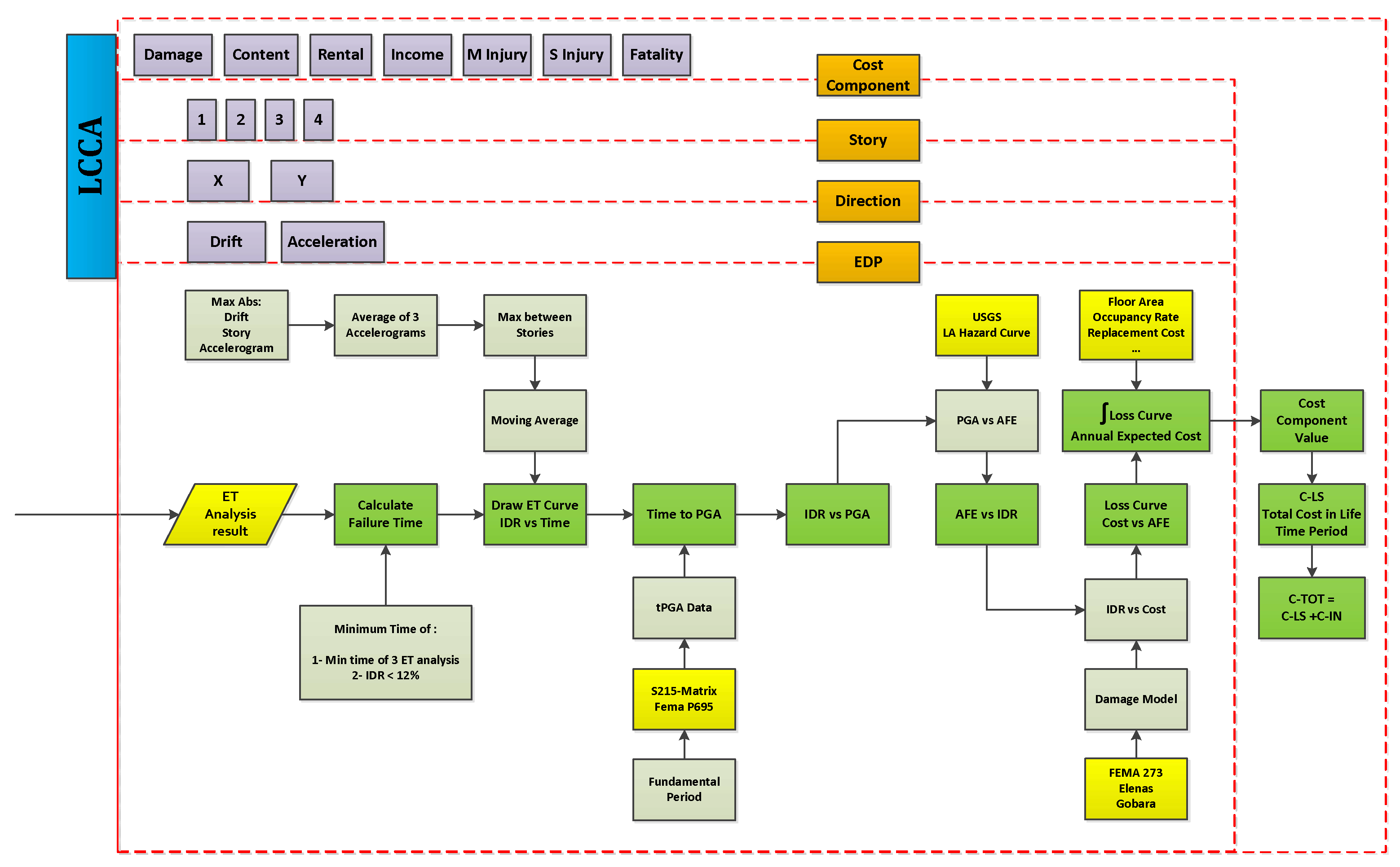
Figure 4.
sections of 3D 4-story RC structure.
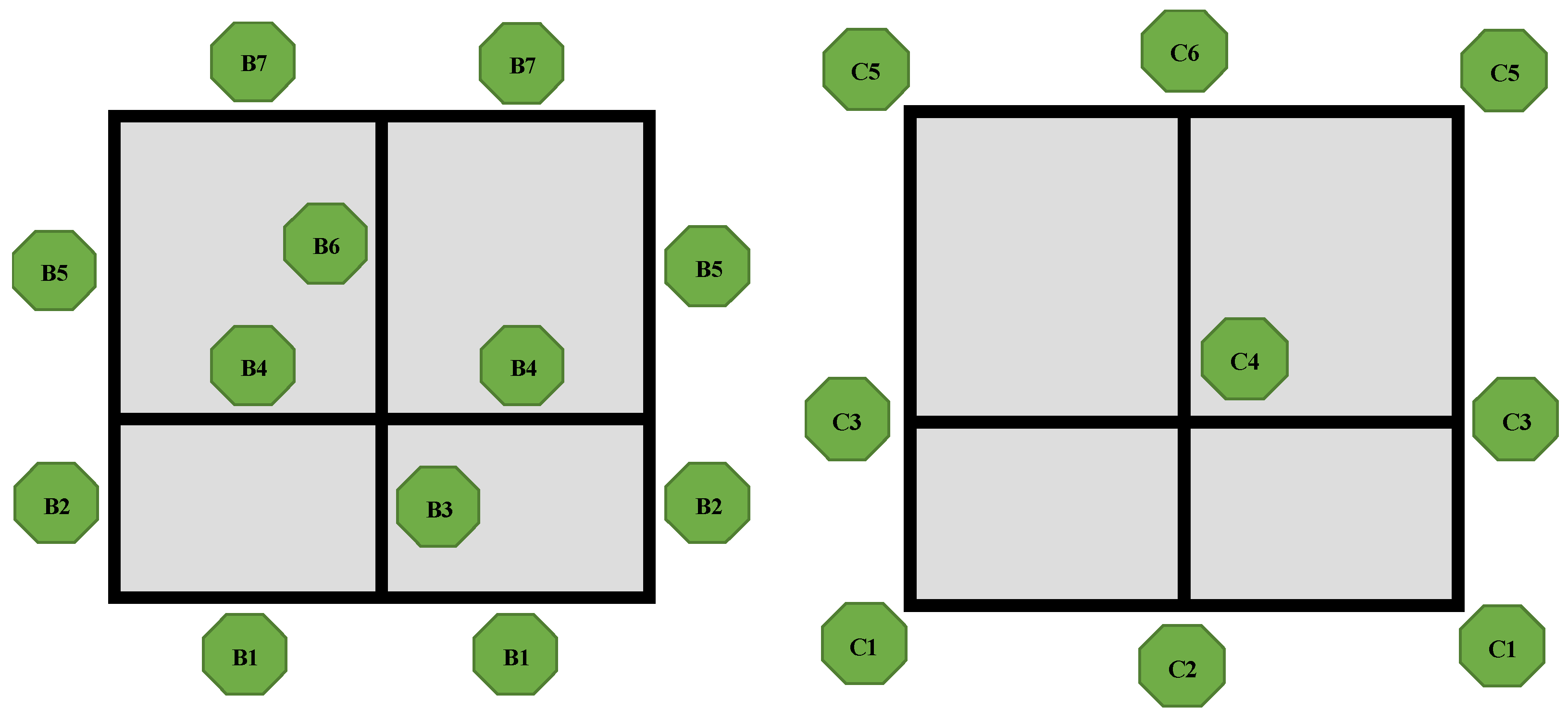
Figure 5.
(a) ET response curves of the code-based and LCCA optimum based designs (b) inter-story drift versus PGA in the code-based and LCCA optimum based designs (c) Loss curve due to drift in direction X for both code-based and LCCA optimum based designs.
Figure 5.
(a) ET response curves of the code-based and LCCA optimum based designs (b) inter-story drift versus PGA in the code-based and LCCA optimum based designs (c) Loss curve due to drift in direction X for both code-based and LCCA optimum based designs.
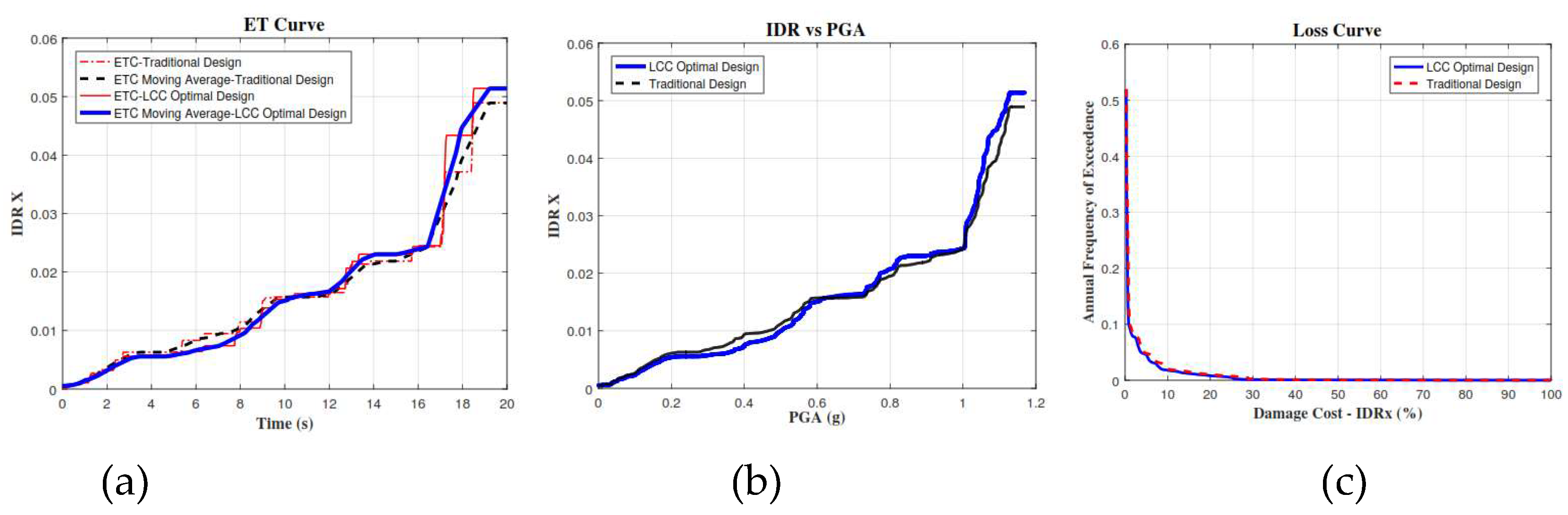
Figure 6.
Optimal Pareto Front obtained from MOIGMM optimization algorithm.
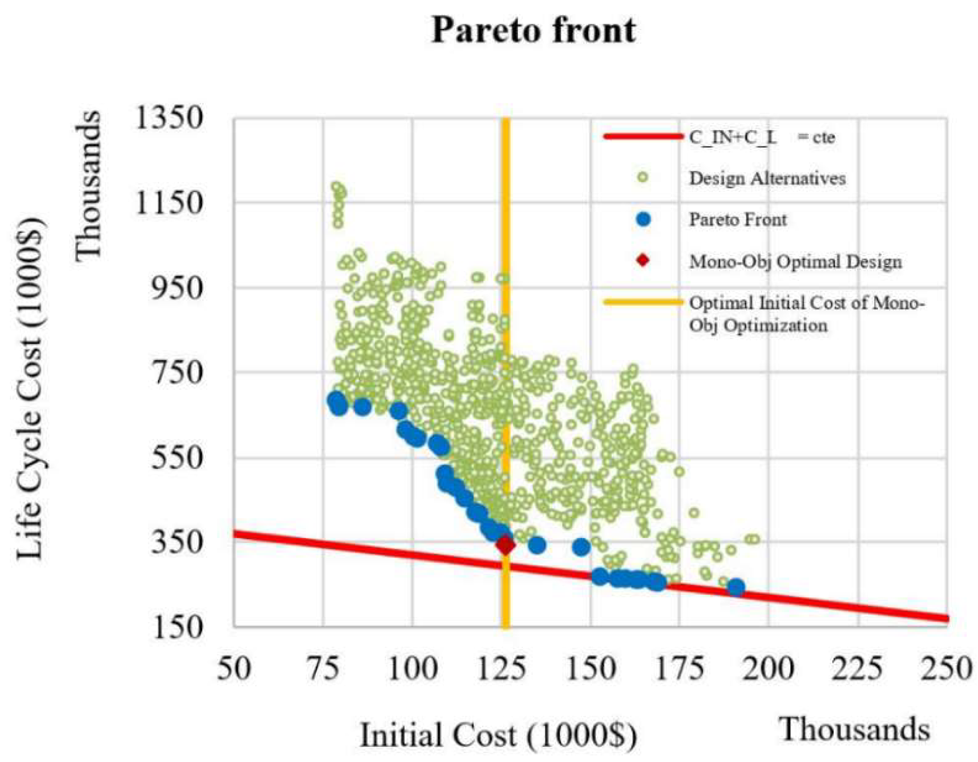
Table 1.
Predefined column sections properties.
| Number | Name | n | (mm) | (cm) | (cm) | (cm2) | (cm2) | (%) |
|---|---|---|---|---|---|---|---|---|
| 1 | C30x30-8T16 | 8 | 16 | 30 | 30 | 16.08 | 900 | 1.79% |
| 2 | C30x30-8T18 | 8 | 18 | 30 | 30 | 20.36 | 900 | 2.26% |
| ... | ... | ... | ... | ... | ... | ... | ... | ... |
| 27 | C45x45-16T20 | 16 | 20 | 45 | 45 | 50.26 | 2025 | 2.48% |
| 28 | C45x45-16T22 | 16 | 22 | 45 | 45 | 60.82 | 2025 | 3.00% |
| ... | ... | ... | ... | ... | ... | ... | ... | ... |
| 65 | C60x60-24-22 | 24 | 22 | 60 | 60 | 91.23 | 3600 | 2.53% |
| 66 | C60x60-24-25 | 24 | 25 | 60 | 60 | 117.81 | 3600 | 3.27% |
Table 2.
Predefined column sections properties.
| Element | Variable | Permissible values |
|---|---|---|
| Column | Column section | 28 first section of Table 1 |
| Beam | Height (cm) | 30, 35, 40, 45 |
| Beam | Relative section areas of the upper bars (%) | 0.35, 0.5, 0.7, 0.8, 1.0, 1.2, 1.4, 1.6, 2.0 |
Table 3.
Comparative information regarding the details of initial cost.
| Initial cost components | Traditional design ($) | LCC based optimal design ($) | Percentage of variation |
|---|---|---|---|
| Column Reinforcement | 13433 | 12961 | -4% |
| Column Concrete | 18931 | 17173 | -9% |
| Column Formwork | 9790.2 | 9595.8 | -2% |
| Beam Reinforcement | 42689 | 43527 | +2% |
| Beam Concrete | 24933 | 27451 | +10% |
| Beam Formwork | 15228 | 15595 | +2% |
| Sum | 125,004 | 126,302 | +1% |
Table 4.
Comparative information regarding the details of life-cycle cost.
| Lifetime cost components | Traditional design($) | LCC based optimal design($) | Percentage of variation |
|---|---|---|---|
| 1.42E+05 | 1.21E+05 | -15% | |
| 47408 | 40171 | -15% | |
| 58914 | 59981 | +2% | |
| 637.49 | 538.41 | -16% | |
| 1.28E+05 | 1.08E+05 | -16% | |
| 71.728 | 55.702 | -22% | |
| 223.76 | 204.26 | -9% | |
| 19937 | 15915 | -20% | |
| Sum | 397,192 | 345,865 | -13% |
Table 5.
Comparative information regarding the details of total life-cycle cost.
| Total cost | Initial cost($) | Lifetime cost($) | Total life-cycle cost($) |
|---|---|---|---|
| Traditional Design | 1.25E+05 | 3.97E+05 | 5.22E+05 |
| LCC Based Optimal Design | 1.26E+05 | 3.45E+05 | 4.71E+05 |
| Percentage of Improvement | +1% | -13% | -10% |
Table 6.
Comparative Eigenvalue results of the code-based and LCCA based design.
| Code based design | LCCA based design | |||||
|---|---|---|---|---|---|---|
| First mode (s) | Second mode (s) | Third mode (s) | First mode (s) | Second mode (s) | Third mode (s) | |
| Period | 0.736 | 0.730 | 0.602 | 0.722 | 0.693 | 0.569 |
| Mode shape | UX | UY | RZ | UX | UY | RZ |
| Story 1 | 0.4563 | 0.4535 | 0.4669 | 0.2986 | 0.3031 | 0.2247 |
| Story 2 | 0.7051 | 0.7014 | 0.7162 | 0.5667 | 0.5716 | 0.4242 |
| Story 3 | 0.8968 | 0.8954 | 0.9046 | 0.8205 | 0.8252 | 0.5983 |
| Story 4 | 1 | 1 | 1 | 1 | 1 | 1 |
Table 7.
Permissible values of design variables for multi-objective optimization.
| Element | Variable | Permissible values |
|---|---|---|
| Column | Column section | All predefined sections from Table 1 |
| Beam | Height (cm) | 30, 35, 40, 45, 50, 55, 60 |
| Beam | Relative section areas of the upper bars (%) | 0.35, 0.40, 0.45, 0.50, 0.60, 0.65, 0.70, 0.75, 0.80, 0.85, 0.90, 0.95, 1.00, 1.10, 1.20, 1.30, 1.40, 1.50, 1.60, 1.80, 2.00 |
Disclaimer/Publisher’s Note: The statements, opinions and data contained in all publications are solely those of the individual author(s) and contributor(s) and not of MDPI and/or the editor(s). MDPI and/or the editor(s) disclaim responsibility for any injury to people or property resulting from any ideas, methods, instructions or products referred to in the content. |
© 2024 by the authors. Licensee MDPI, Basel, Switzerland. This article is an open access article distributed under the terms and conditions of the Creative Commons Attribution (CC BY) license (http://creativecommons.org/licenses/by/4.0/).
Copyright: This open access article is published under a Creative Commons CC BY 4.0 license, which permit the free download, distribution, and reuse, provided that the author and preprint are cited in any reuse.


