Time-travelling Turing Machines and the Self-consistent Halting Problem

Preprint

Article

Time-travelling Turing Machines and the Self-consistent Halting Problem

Altmetrics

Downloads

148

Views

Comments

José Ignacio Orlicki^*

This version is not peer-reviewed

Submitted:

22 September 2024

Posted:

23 September 2024

You are already at the latest version

Alerts

Abstract

This paper introduces the novel concept of Time-Traveling Turing Machines (TTTMs) — Turing Machines with the ability to read symbols that have been explicitly sent from their future computational state. We delve into their properties and behavior, particularly emphasizing the importance of maintaining a self-consistent computational timeline. We present theorems demonstrating the universality of these machines and the challenges in achieving faster computations than traditional Turing Machines.

Keywords:

Subject: Computer Science and Mathematics - Computer Science

1. Introduction

The concept of time travel has long captivated the human imagination, prompting deep questions about causality, paradoxes, and the nature of time itself. While extensively explored in science fiction and philosophy, the computational implications of time travel have received comparatively little attention. This paper aims to bridge that gap by introducing and rigorously analyzing Time-Traveling Turing Machines (TTTMs) - a novel model that extends the capabilities of standard Turing Machines by allowing limited interactions with their own future computational states.

The significance of this work lies in its potential to shed new light on the fundamental limits of computation and the complex interplay between information processing and temporal dynamics. By carefully defining the semantics of time travel within the well-established framework of Turing Machines, we can begin to ask precise questions about the power and limitations of such models, and their relationship to classical notions of computability and complexity.

Our work builds upon a rich tradition of exploring unconventional computation models to gain insights into the nature of information and physical reality. Probabilistic Turing Machines, for example, introduced stochasticity into the deterministic world of classical computation, paving the way for the study of randomized algorithms and cryptography [1]. Quantum Turing Machines took this a step further by harnessing the power of quantum superposition and entanglement, leading to the burgeoning field of quantum computing [2].

Time-Traveling Turing Machines represent a natural next step in this progression. While quantum models leverage the counterintuitive features of quantum mechanics, TTTMs draw inspiration from the equally enigmatic concept of closed timelike curves (CTCs) from relativistic physics [3]. However, unlike most previous studies of CTCs, which focus on their logical consistency and physical plausibility [4], our work adopts a more abstract, algorithmic perspective.

The key novelty of our approach lies in the careful design of the TTTM model to allow only limited, self-consistent interactions with the future. By restricting time travel to the transmission of a single symbol or tape contents, rather than arbitrary computational states, we prevent the most egregious temporal paradoxes while still enabling non-trivial effects. This allows us to prove strong theorems about the expressiveness and efficiency of TTTMs, shedding light on the power of even limited forms of time travel.

Moreover, our work differs from previous studies of hypercomputation and infinite computation [5] in its emphasis on finite, discrete models of time travel. Rather than allowing unlimited computational steps or oracular access to undecidable problems, TTTMs operate within the constraints of classical computability theory, augmented only by self-consistent closed timelike curves. This grounded approach enables us to make precise statements about the relationship between TTTMs and standard complexity classes.

In summary, Time-Traveling Turing Machines represent a significant and novel contribution to the study of unconventional computation models. By carefully extending the classical Turing Machine framework to allow limited forms of time travel, we open up new avenues for exploring the fundamental connections between information, causality, and temporality. Our work thus holds the potential to enrich both theoretical computer science and the broader scientific discourse on the nature of time and computation.

2. Related Work

Historical and contemporary research into unconventional computational models have frequently pushed the boundaries of our understanding. Bennett’s pioneering exploration into logically reversible Turing Machines [6] elucidated the potential for machines that never lose information, leading to the intriguing proposition of thermodynamically reversible computation. This work showed that general-purpose computing automata, such as Turing Machines, can be made logically reversible at every step while retaining their simplicity and ability to perform general computations. The implications of this result are of great physical interest, suggesting the possibility of thermodynamically reversible computers that could perform useful computations at practical speeds while dissipating considerably less than kT of energy per logical step.

Similarly, Probabilistic Turing Machines extended the conventional deterministic computation model, introducing an element of randomness [1]. Gill demonstrated that Probabilistic Turing Machines with small but non-zero error probability can compute certain number-theoretic functions more quickly than deterministic Turing Machines. Additionally, it was shown that Probabilistic Linear-Bounded Automata can simulate Non-Deterministic Linear-Bounded Automata. These results highlight the potential advantages of incorporating randomness into computational models.

Other noteworthy contributions include Predictor Machines [7], which postulate links between predicting the future and emergent complex behaviors. Moore showed that motion with as few as three degrees of freedom can be equivalent to a Turing Machine and thus capable of universal computation. Such systems possess a type of unpredictability qualitatively stronger than that previously discussed in the study of low-dimensional chaos: even if the initial conditions are known exactly, virtually any question about their long-term dynamics is undecidable.

Moreover, quantum computing, with its capability to intertwine communication across various time points through phenomena like entanglement, offers tantalizing glimpses into the union of time and computation. Several models of Universal Quantum Turing Machines have been proposed and analyzed in relation to their physical properties, such as closed timelike curves (CTCs) [2,4,8]. Benioff discussed and reviewed quantum Turing Machines, emphasizing models with Hamiltonians constructed from step operators that include fully quantum mechanical processes taking computation basis states into linear superpositions. Aaronson and Watrous showed that if CTCs existed, quantum computers would be no more powerful than classical computers: both would have the power of the complexity class PSPACE. Khanehsar and Didehvar studied the paradoxical aspects of CTCs and their impact on the theory of computation, proposing axioms to address physical consistency issues and suggesting conditions under which the computational power of CTCs could be realized.

CTCs are a central concept in the study of time travel and its computational implications. The seminal work by Deutsch [9] introduced a model for CTCs that imposes a probabilistic consistency condition to avoid grandfather paradoxes. Aaronson and Watrous [4] built upon this model, studying CTC computers with a polynomial size restriction and showing that they solve exactly the problems in PSPACE, in both the classical and quantum cases. Our work extends these results to the computability setting, where we consider CTCs with no bound on their size. We prove that in this setting, computers with CTCs can solve exactly the problems that are Turing-reducible to the Halting Problem, again in both the classical and quantum cases. This provides a more complete understanding of the computational power of CTCs across different resource bounds.

Another key difference between our work and previous studies of CTCs is the treatment of consistency. In the Deutsch model, CTCs are required to have fixed points (i.e., consistent solutions) for all possible inputs. However, we show that in the computability setting, not all CTCs have fixed points, even probabilistically. Despite this, we prove that the CTCs that do have fixed points are sufficient to have a universal machine that simulates any particular machine of the model. This result highlights the subtle differences between the complexity-theoretic and computability-theoretic perspectives on CTCs.

Hypercomputation, in general, is the study of computational models that are more powerful than Turing Machines, usually incorporating oracles that solve problems and define a hierarchy of machines [5]. Ord surveyed much of the work on hypercomputation, explaining how non-classical models fit into the classical theory of computation and comparing their relative powers. In our case, we introduce a very limited form of oracle that is an operation of sending a symbol from a future configuration into the past configuration of the machine.

Some literature discusses time travel in the context of membrane computing systems [10], focusing on time capsules traveling unchanged from the past to the future, allowing for parallel worlds and the decidability of recursively enumerable languages. However, in our specific model with self-consistent computation histories, decidability of traditional undedidable Turing Machine languages is still not possible. An interesting link between a single finite symbol time traveling and a finite string of symbols has also been explored in the past, with a focus on complexity classes [11]. O’Donnell and Say showed that randomized computation with logarithmically many CTC bits (i.e., polynomially many CTC states) is equivalent to

B P P_{p a t h}

, and quantum computation augmented with logarithmically many classical CTC bits is equivalent to

P P

In contrast to these works, our model of Time-Traveling Turing Machines (TTTMs) focuses on deterministic computation with the ability to send a single symbol back in time. We show that this model is capable of simulating both the Deutsch and postselected CTC models, providing a unified framework for studying the computability aspects of time travel. Furthermore, we introduce the notion of self-consistent computations, which ensures that the outputs of different branches of a TTTM computation agree whenever there are multiple possible timelines. This allows us to define a consistent notion of computation in the presence of time travel, avoiding the grandfather paradox and other logical inconsistencies.

By carefully analyzing the power and limitations of TTTMs, we provide new insights into the relationship between time travel and computation. Our results on the universality of TTTMs and the complexity of simulating them with standard Turing Machines help to delineate the boundaries of what is computable with and without access to time travel. Moreover, by introducing the notions of self-consistent computations and fixed-point solutions, we offer a fresh perspective on the nature of causality and consistency in the context of closed timelike curves.

In summary, our work on Time-Traveling Turing Machines extends and complements the existing literature on unconventional computation, closed timelike curves, and hypercomputation. By focusing on the computability aspects of time travel and introducing novel notions of consistency and simulation, we provide a unified framework for studying the computational power of deterministic systems with access to limited forms of time travel. Our results highlight the subtle interplay between time, information, and computation, opening up new avenues for future research in this exciting area.

3. Definitions

3.1. Traditional Turing Machines

A standard multi-tape, one-sided Turing Machine consists of:

Tape alphabet $Γ$ , with blank symbol ⊔, start symbol ▹.
Set of states Q, initial state $q_{0}$ , halting states $H \subseteq Q$ .
Tape heads, initially positioned at the leftmost cells.
Transition function $δ : Q \times Γ^{k} \to Q \times Γ^{k} \times {L, R}^{k}$ .

The machine operates as follows:

Tape 1 contains the input in cells to the right of ▹. Other tapes have only ▹.
At each step:
- $δ$ uses the current state q and symbols $γ_{1}, \dots, γ_{k}$ under the heads to determine the next state $q^{'}$ , write symbols $γ_{1}^{'}, \dots, γ_{k}^{'}$ , and head moves $D_{1}, \dots, D_{k}$ .
- Heads move left or right, according to $D_{i}$ . They cannot move left from ▹.
- Write $γ_{i}^{'}$ unless it is ▹.
Halting in state $q_{h} \in H$ gives the output: non-blank contents of tape 1.

Tape 1 contains the input and output. Other tapes can be used as scratch space during computation.

Figure 1 illustrates a traditional Turing Machine with input "abc" on tape 1 and scratch work on tape 2. The machine’s state and tape head positions are updated according to the transition function

δ

at each step of the computation.

3.2. Single Symbol Time-Traveling Turing Machine

A Single Symbol Time-Traveling Turing Machine (SSTTM) augments the standard model with the following:

Tape 1 holds a non-negative integer S in binary using all symbols except blank.
Tape 2 holds the input and scratch workspace.
Special internal state $q_{send} \in Q$ to send a symbol back in time.

The machine operates as follows:

Computation proceeds as normal, except tape 1 holds the "time lag" S.
Upon entering $q_{send}$ , the symbol $γ$ under the tape 2 head is sent S steps back in time on tape 2.
If the current timestep $t < S$ , the machine transitions to a special error state $q_{error} \notin H$ .
Otherwise, $γ$ is placed on tape 2 at the same position corresponding to past configuration in timestep $t - S$ , overwriting the symbol that was there.
Computation continues in timestep $t - S$ from $q_{send}$ , potentially in a new timeline.
As before, halting in H gives the output from tape 1.

This allows a single tape 2 symbol to be sent into the past, determined by the time lag S on tape 1.

Figure 2 depicts a SSTTM sending a symbol back in time. The time lag S is encoded on tape 1, and the symbol

γ

under the tape 2 head is sent S steps into the past, potentially creating a new timeline.

3.3. Internal Clock Time-Traveling Turing Machine

An Internal Clock Time-Traveling Turing Machine (ICTTM) has:

Internal timestamp counter C incrementing at each step.
Special state $q_{send} \in Q$ to optionally send the tape 1 symbol to time 0.

The machine operates as follows:

C starts at 0 and increments at each timestep.
Computation proceeds normally until optionally entering $q_{send}$ .
Upon entering $q_{send}$ , the current tape 1 symbol is sent to the same tape position at time 0, overwriting what was there.
Computation continues from $q_{send}$ .
Halting gives the output on tape 1.

Figure 3 illustrates an ICTTM sending a symbol to time 0. The internal timestamp counter C keeps track of the current timestep, and upon entering

q_{send}

, the current tape 1 symbol is sent to the same position at time 0.

Theorem 1.

Any Internal Clock Time-Traveling Turing Machine (ICTTM) can be simulated by a Single Symbol Time-Traveling Turing Machine (SSTTM) using an additional scratch tape.

Proof.

Let M be an ICTTM with tape alphabet

Γ

, states Q, initial state

q_{0}

, halting states H, and transition function

δ

. We construct an SSTTM

M^{'}

that simulates M as follows:

$M^{'}$ has tape alphabet $Γ^{'} = Γ \cup {(γ, q, d) ∣ γ \in Γ, q \in Q, d \in {L, R}}$ , where the additional symbols encode the tape contents, head position, and state of M at each step.
$M^{'}$ has states $Q^{'} = Q \cup {q_{sim}, q_{send}^{'}, q_{retrieve}, q_{write}}$ , where $q_{sim}$ is used for simulating M, $q_{send}^{'}$ is used for sending symbols back in time, $q_{retrieve}$ is used for retrieving the sent symbol, and $q_{write}$ is used for writing the retrieved symbol to the simulated tape of M.
$M^{'}$ has initial state $q_{0}$ and halting states $H^{'} = H$ .
$M^{'}$ uses tape 1 for the time lag and tape 2 for simulating the tape of M and encoding the computational history.

The simulation proceeds as follows:

$M^{'}$ starts in state $q_{0}$ with input w on tape 2 and time lag S on tape 1.
In state $q_{sim}$ , $M^{'}$ simulates one step of M using the transition function $δ$ . It updates the current state, tape contents, and head position on tape 2 according to $δ$ .
After each simulated step, $M^{'}$ writes the current tape symbol $γ$ , state q, and head direction d as $(γ, q, d)$ to the scratch tape to record the computational history.
If M enters state $q_{send}$ , $M^{'}$ transitions to state $q_{send}^{'}$ and sets its time lag on tape 1 to the binary encoding of the current step number C.
In state $q_{send}^{'}$ , $M^{'}$ sends the current symbol on tape 2 back C steps in time. It then moves the head to the position on tape 2 corresponding to time 0.
$M^{'}$ transitions to state $q_{retrieve}$ and reads the symbol $(γ, q, d)$ from the scratch tape at the position corresponding to time 0.
$M^{'}$ transitions to state $q_{write}$ , writes $γ$ to tape 2, moves the head in direction d, and updates the current state to q.
$M^{'}$ transitions back to state $q_{sim}$ and continues the simulation of M.
If M enters a halting state in H, $M^{'}$ also halts, and its output is the contents of tape 2, which represents the final tape of M.

To illustrate the simulation, consider an example ICTTM M with the following behavior:

M starts with input "01" on its tape.
At step 3, M enters state $q_{send}$ and sends the current symbol "1" to time 0.
M continues its computation and halts at step 5 with output "11".

The SSTTM

M^{'}

simulates M as follows:

$M^{'}$ starts with input "01" on tape 2 and time lag 3 (binary "11") on tape 1.
$M^{'}$ simulates steps 1 and 2 of M in state $q_{sim}$ , writing the computational history to the scratch tape: "(0, $q_{0}$ , R)", "(1, $q_{1}$ , R)".
At step 3, M enters $q_{send}$ , so $M^{'}$ transitions to $q_{send}^{'}$ and sends the current symbol "1" back 3 steps in time.
$M^{'}$ moves the head on tape 2 to the position corresponding to time 0, transitions to $q_{retrieve}$ , and reads "(0, $q_{0}$ , R)" from the scratch tape.
$M^{'}$ transitions to $q_{write}$ , writes "1" to tape 2, moves the head right, and updates the current state to $q_{0}$ . The scratch tape now contains "(1, $q_{0}$ , R)" at the position corresponding to time 0.
$M^{'}$ transitions back to $q_{sim}$ and continues simulating M from state $q_{0}$ with tape contents "11".
$M^{'}$ simulates steps 4 and 5 of M, writing the computational history to the scratch tape: "(1, $q_{2}$ , R)", "(1, $q_{3}$ , R)".
At step 5, M enters a halting state, so $M^{'}$ also halts with output "11" on tape 2.

This step-by-step breakdown demonstrates how the SSTTM

M^{'}

uses its scratch tape to encode the full computational history of the ICTTM M and correctly simulates the internal clock send operation. By recording the tape contents, head position, and state at each step,

M^{'}

can accurately update the simulated tape of M when a symbol is sent back in time, ensuring a faithful simulation of the ICTTM. □

This shows that the internal clock model can be simulated by a single symbol time traveler, demonstrating that the latter is at least as powerful as the former.

3.4. Full Tape ICTTM

A Full Tape Internal Clock Time-Traveling Turing Machine has:

Internal counter C incremented each step.
State $q_{send}$ to send all non-blank contents of tape 1 to time 0.

It operates as follows:

C increments each timestep.
Upon entering $q_{send}$ , the entire current non-blank contents of tape 1 are sent to the same positions at time 0, overwriting what was there.
Computation continues from $q_{send}$ .
Halting gives the output on tape 1.

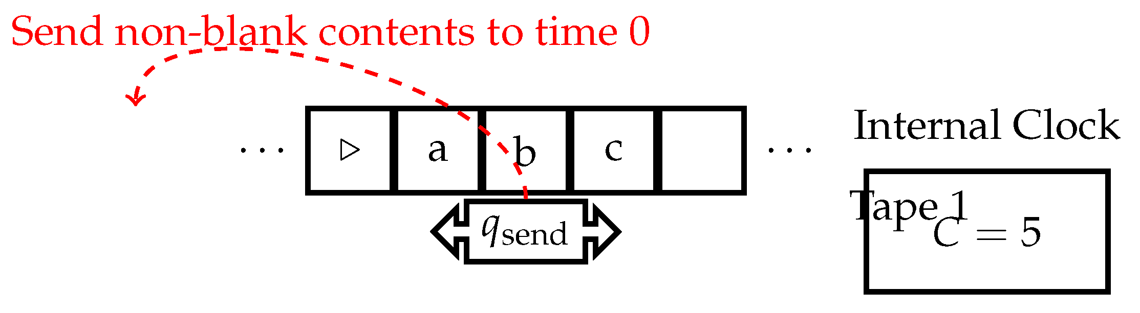
Figure 4 depicts a Full Tape ICTTM sending the entire non-blank contents of tape 1 to time 0. Upon entering

q_{send}

, all non-blank symbols on tape 1 are sent to their corresponding positions at time 0, overwriting the previous contents.

Theorem 2.

The Full Tape ICTTM can be simulated by a Single Symbol ICTTM.

Proof.

Let M be a Full Tape ICTTM with tape alphabet

Γ

, states Q, initial state

q_{0}

, halting states H, and transition function

δ

. We construct a Single Symbol ICTTM

M^{'}

that simulates M as follows:

$M^{'}$ has tape alphabet $Γ^{'} = Γ \cup {(γ, i) ∣ γ \in Γ, i \in N}$ , where the additional symbols encode the tape contents and their positions at each step.
$M^{'}$ has states $Q^{'} = Q \cup {q_{sim}, q_{send}^{'}, q_{iterate}, q_{retrieve}, q_{write}}$ , where $q_{sim}$ is used for simulating M, $q_{send}^{'}$ is used for initiating the sending of symbols back in time, $q_{iterate}$ is used for iterating through the scratch tape history, $q_{retrieve}$ is used for retrieving the sent symbol, and $q_{write}$ is used for writing the retrieved symbol to the simulated tape of M.
$M^{'}$ has initial state $q_{0}$ and halting states $H^{'} = H$ .
$M^{'}$ uses tape 1 for simulating the tape of M and encoding the computational history, and a scratch tape for storing the symbols and their positions to be sent back in time.

The simulation proceeds as follows:

$M^{'}$ starts in state $q_{0}$ with input w on tape 1.
In state $q_{sim}$ , $M^{'}$ simulates one step of M using the transition function $δ$ . It updates the current state, tape contents, and head position on tape 1 according to $δ$ .
After each simulated step, $M^{'}$ writes the current tape symbol $γ$ and its position i as $(γ, i)$ to the scratch tape to record the computational history.
If M enters state $q_{send}$ , $M^{'}$ transitions to state $q_{send}^{'}$ and moves the head to the beginning of the scratch tape.
In state $q_{iterate}$ , $M^{'}$ iterates through the scratch tape, reading each symbol $(γ, i)$ one at a time.
For each $(γ, i)$ , $M^{'}$ moves the head on tape 1 to position i, transitions to state $q_{send}$ , and sends $γ$ back to time 0 at position i.
$M^{'}$ then moves the head back to the scratch tape, transitions to state $q_{retrieve}$ , and reads the next symbol $(γ^{'}, i^{'})$ .
$M^{'}$ transitions to state $q_{write}$ , moves the head on tape 1 to position $i^{'}$ , writes $γ^{'}$ , and transitions back to state $q_{iterate}$ .
After processing all symbols on the scratch tape, $M^{'}$ transitions back to state $q_{sim}$ and continues the simulation of M.
If M enters a halting state in H, $M^{'}$ also halts, and its output is the contents of tape 1, which represents the final tape of M.

The runtime overhead of this simulation is

O (n^{2})

, where n is the number of steps in the computation of M. This is because for each step of M,

M^{'}

needs to iterate through the entire scratch tape history, which grows linearly with the number of steps. The space overhead is

O (n)

, as the scratch tape needs to store the tape contents and their positions at each step.

To illustrate the simulation, consider an example Full Tape ICTTM M with the following behavior:

M starts with input "01" on its tape.
At step 3, M enters state $q_{send}$ and sends the entire non-blank contents of the tape, "011", back to time 0.
M continues its computation and halts at step 5 with output "0111".

The Single Symbol ICTTM

M^{'}

simulates M as follows:

$M^{'}$ starts with input "01" on tape 1.
$M^{'}$ simulates steps 1 and 2 of M in state $q_{sim}$ , writing the computational history to the scratch tape: "(0, 0)", "(1, 1)".
At step 3, M enters $q_{send}$ , so $M^{'}$ transitions to $q_{send}^{'}$ and moves the head to the beginning of the scratch tape.
$M^{'}$ transitions to $q_{iterate}$ and reads the first symbol "(0, 0)" from the scratch tape.
$M^{'}$ moves the head on tape 1 to position 0, transitions to $q_{send}$ , and sends "0" back to time 0 at position 0.
$M^{'}$ moves the head back to the scratch tape, transitions to $q_{retrieve}$ , and reads the next symbol "(1, 1)".
$M^{'}$ transitions to $q_{write}$ , moves the head on tape 1 to position 1, writes "1", and transitions back to $q_{iterate}$ .
$M^{'}$ reads the next symbol "(1, 2)" from the scratch tape, moves the head on tape 1 to position 2, transitions to $q_{send}$ , and sends "1" back to time 0 at position 2.
After processing all symbols on the scratch tape, $M^{'}$ transitions back to $q_{sim}$ and continues simulating M from time 0 with tape contents "011".
$M^{'}$ simulates steps 4 and 5 of M, writing the computational history to the scratch tape: "(1, 3)".
At step 5, M enters a halting state, so $M^{'}$ also halts with output "0111" on tape 1.

This detailed proof and example demonstrate how the Single Symbol ICTTM

M^{'}

simulates the Full Tape ICTTM M by iterating through the scratch tape history and sequentially sending each symbol back in time to its original position. The analysis of the runtime and space overheads provides insight into the efficiency of this simulation. □

This demonstrates that the Full Tape model can also be simulated by a Single Symbol Time Traveler. We use the Single Symbol Time-Traveling Turing Machine model as the foundational model, but we have proved that many other models can be simulated with the foundational one.

4. Properties

4.1. Self-Consistent Computability

The ability of Single Symbol Time-Traveling Turing Machines (SSTTMs) to send tape symbols into the past introduces non-determinism and potential timeline bifurcations. We formalize the notion of a self-consistent computation and output, drawing inspiration from Novikov’s self-consistency principle, which states that the only possible time travel scenarios are those that do not lead to logical contradictions or paradoxes [3].

Definition 1.

Let M be an SSTTM, and let

s_{1}, s_{2}, \dots, s_{k}

be the sequence of symbols sent to the past by M during its computation on input w. Sending each symbol

s_{i}

results in either 0 or 1 new bifurcations in the computation history of M, denoted as:

$b (s_{i}) = 0$ if $s_{i}$ does not cause a new bifurcation
$b (s_{i}) = 1$ if $s_{i}$ causes a single new bifurcation

Let

O_{1}, O_{2}, \dots, O_{r}

be the set of all possible outputs printed on tape 2 from the r many bifurcations caused by sending symbols into the past during the computation of

M (w)

Then, the computation of

M (w)

is said to be self-consistent if:

$k = 0$ , i.e., no symbols are sent to the past by $M (w)$ , and $M (w)$ halts normally with output $O_{1}$ .
$k > 0$ , i.e., symbols are sent to the past, causing bifurcations, but $O_{1} = O_{2} = \dots = O_{r}$ . That is, all branches halt with the same output on tape 2. We consider this a halting computation with the common output.
If there exist l and m such that the outputs of halting branches are not equal, $O_{l} \neq O_{m}$ , then we consider this computation to be non-halting.

Intuitively, a self-consistent computation has only one possible output, despite any apparent non-determinism from time travel. This definition ensures that the computation respects Novikov’s self-consistency principle, avoiding paradoxes or contradictions that could arise from sending symbols back in time.

To illustrate these concepts, consider the following examples:

Example 1

(Consistent Computation). Let M be an SSTTM with the following behavior on input "01":

At step 3, M sends the symbol "1" back to step 1, overwriting the original "0".
M continues its computation and halts at step 5 with output "11".

This computation is self-consistent because there is only one possible output, "11", regardless of the bifurcation caused by sending the symbol back in time. The branch that starts with the original input "01" will also halt with output "11" after receiving the symbol "1" from the future.

Example 2

(Inconsistent Computation). Let M be an SSTTM with the following behavior on input "01":

At step 3, M sends the symbol "0" back to step 1, overwriting the original "0".
At step 4, M sends the symbol "1" back to step 2, overwriting the original "1".
The branch that starts with the original input "01" halts at step 5 with output "00".
The branch that receives the symbol "0" at step 1 halts at step 5 with output "01".

This computation is inconsistent because the two branches halt with different outputs, "00" and "01". The sending of symbols back in time has created a paradox, violating Novikov’s self-consistency principle.

We can now define the output of a self-consistent computation. For a given SSTTM M:

If M has a unique timeline with no time travel, the output is the tape 2 contents upon halting.
If M bifurcates timelines by time travel, the output is the common tape 2 contents across all branches when halting.
If M bifurcates timelines by time travel but some branches have different traditional outputs, we consider the self-consistent computation to be non-halting or entering an error or rejecting state.

Theorem 3.

Checking that an output has been found in a self-consistent SSTTM computation within n finite steps can be finitely decided by a traditional Turing Machine within also a finite number of steps.

Proof.

Let M be an SSTTM, and w be an input. We will construct a traditional Turing Machine T that can decide in finite time whether M has a consistent output on w across all bifurcations with n or fewer steps.

T will simulate the computation tree of M on w in a breadth-first manner, tracking tape contents at each timestep in each branch.

Formally, T operates as follows:

Create an initial configuration $C_{0}$ of M on input w.
Set list $L = [C_{0}]$ to track configurations.
While L is non-empty:
(a)

Remove the first configuration C from L.

(b)

Simulate one step of C to generate configurations $C^{'}$ .

(c)
If C halts, compare the output tape to C’s previously saved output tape.
If equal, continue to the next C.

If unequal, reject.
(d)

Add all $C^{'}$ to the end of L.
If L empties with no rejection, accept.

Observe:

Each C depends only on its parent configuration, so T can correctly recreate C.
The branching factor of M is finite, so $| L |$ is at most exponential in runtime.

Therefore, as L is finite, T will eventually simulate all configurations of M on w and detect any inconsistencies or accept. As T only needs to track a finite number of configurations, this process terminates in finite time.

This shows T can decide finitely if M has a consistent output across bifurcations within finite n steps. □

This formalization of self-consistency, along with the concrete examples and the connection to Novikov’s self-consistency principle, provides a clearer understanding of what constitutes a valid output for an SSTTM computation involving time travel. The theorem and proof demonstrate that checking for self-consistency within a finite number of steps is decidable by a traditional Turing Machine, ensuring that the notion of self-consistent computability is well-defined and computable.

This also formalizes which solutions we consider valid outputs of an SSTTM computation involving time travel. Even with timeline bifurcations, a self-consistent output requires agreement between all branches. Consistency guarantees a well-defined result, avoiding paradoxes from contradictory outputs. The problem with self-consistent computations is that they do not seem computable to decide if you are on a halting state that is part of a self-consistent computation without simulating all the bifurcations, but we will see if we can prove this is computable in our model. This means that there is a Universal SSTTM that is properly utilizing the time-traveling internal state to simulate any of the possible SSTTMs.

Theorem 4.

There exists a Universal SSTTM U that has a self-consistent output indicating whether a given SSTTM M has a self-consistent computation.

Proof.

Let U be a Universal SSTTM, and M be an arbitrary SSTTM that U takes as input. We will show that U can generate a self-consistent output indicating whether M has a self-consistent computation on input w.

U simulates the computation tree of

M (w)

in a breadth-first manner, keeping track of tape contents across all branches.

Formally, the operation of U is:

Universal SSTTM U:

1. C_0 ← initial configuration of M(w)

2. L ← [C_0]

3. while L is not empty:

4. C ← L.dequeue()

5. C’ ← simulate_one_step(C)

6. if C halts:

7. o_C ← get_output_tape(C)

8. send_to_all_prior_branches(o_C)

9. for each branch point B:

10. if o_C = o_B:

11. continue

12. else:

13. halt in state q_inconsistent

14. L.enqueue_all(C’)

15. if L is empty:

16. halt in state q_consistent

We observe:

The branching factor of M is finite as it is an SSTTM. Thus, $| L |$ is at most exponential in the runtime, i.e., $| L | \leq c^{t}$ for some constant c and runtime t.
U can correctly recreate any configuration C from its parent.
As L is finite, U will eventually simulate all possible configurations of $M (w)$ .

The number of simulation steps performed by U is bounded by the total number of configurations in the computation tree of

M (w)

. In the worst case, this is exponential in the runtime of M, i.e.,

O (c^{t})

for some constant c and runtime t. The size of each configuration is bounded by the size of M and the length of the input w, i.e.,

O (| M | + | w |)

Therefore, as U simulates all branches and compares outputs at each branch point, it will definitively enter either

q_{consistent}

M (w)

is self-consistent, or

q_{inconsistent}

if not. The total runtime of U is bounded by

O (c^{t} \cdot (| M | + | w |))

, which is exponential in the runtime of M and linear in the size of M and w.

Thus, U generates a self-consistent output indicating if

M (w)

is self-consistent across all bifurcations. □

This demonstrates that consistency can be checked within the SSTTM model itself. The potentially unbounded branching is handled by harnessing time travel to share information across timelines. Also, the potentially unbounded branching makes the consistency of these computations, which is akin to a Halting Problem, undecidable by a traditional deterministic Turing Machine. We can simulate time bifurcations in a traditional Turing Machine by exploring them either in a depth-first or breadth-first manner and using the dovetailing technique, but we can prove that the number of bifurcations can be unbounded and undecidable in the traditional model.

Theorem 5.

Given an SSTTM M, it is undecidable by a traditional Turing Machine whether simulating M results in a finite or infinite number of bifurcations.

Proof.

Let us assume for contradiction that there exists a traditional Turing Machine T that can determine if the simulation of an arbitrary SSTTM M on input w results in a finite or infinite number of bifurcations. Consider the set

S = {〈 M, w 〉}

of all possible pairs of an SSTTM M and input w. We can enumerate this set as

S = {〈 M_{1}, w_{1} 〉, 〈 M_{2}, w_{2} 〉, \dots}

. We will construct a diagonalizing SSTTM N that takes as input a pair

〈 M_{i}, w_{i} 〉

and behaves as follows:

N simulates T on input $〈 M_{i}, w_{i} 〉$ to obtain T’s prediction of whether $M_{i}$ on input $w_{i}$ will result in a finite or infinite number of bifurcations.
If T predicts that $M_{i}$ on input $w_{i}$ will result in a finite number of bifurcations, N simulates $M_{i}$ on input $w_{i}$ but introduces a time travel paradox that causes an infinite number of bifurcations. N achieves this by sending a symbol back in time that contradicts the symbol that was originally present at that position, creating a scenario similar to the grandfather paradox. This contradiction leads to an infinite number of bifurcations, each corresponding to a different resolution of the paradox.
If T predicts that $M_{i}$ on input $w_{i}$ will result in an infinite number of bifurcations, N simulates $M_{i}$ on input $w_{i}$ without introducing any additional time travel. In this case, N will have the same number of bifurcations as $M_{i}$ , which is finite.

The construction of N is analogous to the classic diagonalization technique used in proofs of undecidability, such as the proof of the undecidability of the Halting Problem. In that proof, a diagonalizing Turing Machine is constructed that takes as input the description of a Turing Machine and its input, and behaves differently than the input machine on that input. This leads to a contradiction when the diagonalizing machine is given its own description as input.

Similarly, our diagonalizing SSTTM N takes as input a pair

〈 M_{i}, w_{i} 〉

and behaves differently than

M_{i}

on input

w_{i}

with respect to the number of bifurcations, based on the prediction of the assumed deciding machine T. This leads to a contradiction when N is given its own description and input as a pair

〈 N, 〈 N, w 〉 〉

If T predicts that N on input

〈 N, w 〉

will result in a finite number of bifurcations, then N will introduce a time travel paradox causing an infinite number of bifurcations. Conversely, if T predicts that N on input

〈 N, w 〉

will result in an infinite number of bifurcations, then N will not introduce any additional time travel, resulting in a finite number of bifurcations. In either case, N behaves differently than predicted by T, contradicting the assumption that T can correctly decide whether an SSTTM on a given input will result in a finite or infinite number of bifurcations.

Therefore, by contradiction, there cannot exist a traditional Turing Machine T that can determine if the simulation of an arbitrary SSTTM M on input w will result in a finite or infinite number of bifurcations. The problem of predicting whether an SSTTM will have a finite or infinite number of bifurcations is undecidable. □

The core issue is that simulating all possible branches of an SSTTM to count bifurcations is infeasible on a traditional Turing Machine. By harnessing time travel, SSTTMs can share information across branches, but this capability cannot be reproduced without it.

4.2. Complexity Constraints

Theorem 6.

Let M be a traditional Turing Machine running in time

T (n)

on input x. Construct an SSTTM

M^{'}

which simulates M on x, sends x paired with the output back in time, then halts also with the correct output. In the worst-case complexity,

M^{'}

must still run in

Ω (T (n))

time to be self-consistent.

Proof.

Let M be a traditional Turing Machine with time complexity

T (n)

on inputs of length n. We construct an SSTTM

M^{'}

that operates as follows on input x of length n:

$M^{'}$ simulates $M (x)$ for $T (n)$ steps, recording the output as o.
At the end of the simulation, $M^{'}$ sends the pair $〈 x, o 〉$ back in time to the initial configuration.
$M^{'}$ then halts with output o.

This creates two branches in the timeline of

M^{'}

The original branch $B_{1}$ where $M (x)$ is simulated for the full $T (n)$ steps before $M^{'}$ halts.
The new branch $B_{2}$ starting with the output pair $〈 x, o 〉$ sent back in time.

To ensure a self-consistent output o, the computation in branch

B_{1}

must fully complete. This occurs with probability p, where p is the probability that

M^{'}

starts in the original timeline.

The key observations are:

The worst-case runtime of branch $B_{1}$ is $T (n)$ to simulate $M (x)$ .
The runtime of branch $B_{2}$ is constant as it starts with the output.
To be self-consistent, the output o must be produced in full in branch $B_{1}$ .

Therefore, the worst-case expected runtime of

M^{'}

across branches is

Ω (T (n))

. The potential speedup of branch

B_{2}

does not improve this worst-case bound due to the need for self-consistency with branch

B_{1}

Now, let’s consider the average-case runtime of

M^{'}

under some assumptions about the branch probability distribution. Suppose that the probability of starting in branch

B_{1}

is p and the probability of starting in branch

B_{2}

1 - p

. The average-case runtime of

M^{'}

can be expressed as:

\begin{matrix} E [runtime (M^{'})] & = p \cdot T (n) + (1 - p) \cdot O (1) \\ = p \cdot T (n) + O (1) \end{matrix}

If p is a constant (independent of n), then the average-case runtime of

M^{'}

Θ (T (n))

, which is asymptotically the same as the worst-case runtime. This suggests that, under a uniform branch probability distribution, the average-case runtime of

M^{'}

is still constrained by the need for self-consistency with branch

B_{1}

However, if p is allowed to depend on n, then the average-case runtime of

M^{'}

could potentially be improved. For example, if

p = O (1 / T (n))

, then the average-case runtime of

M^{'}

would be:

\begin{matrix} E [runtime (M^{'})] & = O (1 / T (n)) \cdot T (n) + O (1) \\ = O (1) \end{matrix}

In this case, the average-case runtime of

M^{'}

would be constant, representing a significant speedup over the worst-case runtime. However, it is important to note that this speedup comes at the cost of a reduced probability of self-consistency, as the probability of starting in branch

B_{1}

decreases with n. □

These observations suggest that the complexity constraints on SSTTMs can be sensitive to assumptions about the branch probability distribution. While the worst-case runtime is always constrained by the need for self-consistency, the average-case runtime may be improved under certain probability distributions that favor faster branches. However, this improvement in average-case runtime comes at the cost of a reduced probability of self-consistency.

Further research could explore the trade-offs between average-case runtime and the probability of self-consistency under different branch probability distributions. This could lead to a more nuanced understanding of the complexity constraints on SSTTMs and the potential for leveraging time travel to achieve speedups in specific scenarios.

In summary, because only branches that complete the original

T (n)

computation can produce self-consistent output, probabilistic speedups in worst-case complexity cannot be obtained through time travel in this model.

5. Conclusions

Time-Traveling Turing Machines provide a fascinating framework to investigate the interplay between computation, consistency, and time. Our exploration suggests that while these machines hold potential, they are bound by certain constraints, especially ensuring self-consistent timelines. Further research is needed to unlock their full potential and address the myriad of challenges they present.

In this paper, we introduced Time-Traveling Turing Machines and rigorously characterized their properties. We defined several models enabling limited forms of sending information back in time and formalized the notion of consistency for computations involving time travel.

Our main results are:

Single Symbol Time-Traveling Turing Machines (SSTTMs) can simulate other restricted models like Internal Clock Time-Traveling Turing Machines and also models with arbitrary size data traveling. This establishes a robust foundation for studying temporal effects in computation.
Determining computational consistency is possible within the SSTTM model itself. We have Universal SSTTMs that can function as watchers and controllers of SSTTM consistency. The ability to send outputs back in time allows verifying correctness across branches.
Requiring self-consistent outputs prohibits using time travel to speed up computation in the worst-case time complexity. We cannot restrict a longer computation into a shorter computation by removing some of the parallel time bifurcations.

Together, these findings help connect concepts of computation, time, prediction, and complexity. However, our current models have several limitations that present opportunities for further research:

Our models only allow sending limited symbols or tape contents back in time. Extending the model to allow more general message passing, such as sending entire programs or algorithms, could reveal new insights into the relationship between time travel and computational complexity. For example, what are the implications of sending optimized machines from the future back in time? This could lead to new connections between time travel, compression, and algorithmic information theory.
Our models focus on deterministic computation with a limited form of non-determinism introduced by time travel. Exploring the interplay between time travel and other forms of non-determinism, such as probabilistic or quantum computation, could yield new insights into the nature of computation and the role of time. For example, how does the introduction of time travel affect the computational power of Probabilistic or Quantum Turing Machines?
Our models consider time travel within a single computational system. Extending the model to allow interactions between multiple SSTTMs could lead to new questions about the nature of causality, consistency, and communication in the presence of time travel. For example, how can multiple SSTTMs coordinate to achieve a common computational goal while maintaining consistency across their respective timelines?

In addition to these limitations and open problems, it is worth considering how our models of Time-Traveling Turing Machines relate to other notions of closed timelike curves (CTCs) and hypercomputation. CTCs have been studied extensively in the context of physics and have been shown to enable hypercomputation in certain models of computation, such as Malament-Hogarth spacetimes and Kerr black holes [12]. However, these models often rely on specific assumptions about the nature of spacetime and the availability of infinite computational resources.

Our models of SSTTMs, in contrast, focus on the computational implications of time travel within the framework of classical Turing Machines. While we have shown that SSTTMs can simulate certain restricted models of hypercomputation, such as Internal Clock Time-Traveling Turing Machines, our results also highlight the limitations of using time travel to achieve speedups in computation. In particular, our results on the complexity constraints of SSTTMs suggest that time travel alone may not be sufficient to achieve arbitrary levels of hypercomputation, at least within the framework of classical computation.

Further research could explore the connections between SSTTMs and other models of hypercomputation, such as Oracle Machines and Infinite Time Turing Machines[13].This could lead to a more comprehensive understanding of the computational power of time travel and its relationship to other forms of non-classical computation.

Overall, Time-Traveling Turing Machines establish a new lens for investigating the interplay between computational theory and concepts of time, causality, and temporal logic. By formalizing the notion of consistency in the presence of time travel and studying the computational power of SSTTMs, we have opened up new avenues for research at the intersection of computer science, physics, and philosophy. We hope that this work will inspire further exploration of the fascinating and perplexing questions that arise when computation and time travel collide.

Acknowledgments

The author would like to thank the support of Trust Machines (Nassau Machines Inc.).

References

Gill, J.T. Computational Complexity of Probabilistic Turing Machines. Proceedings of the Sixth Annual ACM Symposium on Theory of Computing; Association for Computing Machinery: New York, NY, USA, 1974; STOC’74; pp. 91–95. [Google Scholar]
Benioff, P. Models of Quantum Turing Machines. Fortschritte der Physik 1998, 46, 423–441. [Google Scholar] [CrossRef]
Novikov, I.D. Time machine and self-consistent evolution in problems with self-interaction. Phys. Rev. D 1992, 45, 1989–1994. [Google Scholar] [CrossRef] [PubMed]
Aaronson, S.; Watrous, J. Closed timelike curves make quantum and classical computing equivalent. Proceedings of the Royal Society A: Mathematical, Physical and Engineering Sciences 2008, 465, 631–647. [Google Scholar] [CrossRef]
Ord, T. Hypercomputation: computing more than the Turing machine. arXiv 2002, arXiv:math.LO/math/0209332. [Google Scholar]
Bennett, C.H. Logical Reversibility of Computation. IBM Journal of Research and Development 1973, 17, 525–532. [Google Scholar] [CrossRef]
Moore, C. Unpredictability and undecidability in dynamical systems. Phys. Rev. Lett. 1990, 64, 2354–2357. [Google Scholar] [CrossRef] [PubMed]
Khanehsar, S.B.; Didehvar, F. Turing Machines Equipped with CTC in Physical Universes. CoRR 2023, abs/2301.11632. [Google Scholar]
Deutsch, D. Quantum mechanics near closed timelike lines. Phys. Rev. D 1991, 44, 3197–3217. [Google Scholar] [CrossRef]
Freund, R.; Ivanov, S. How to Go Beyond Turing with P Automata: Time Travels, Regular Observer w-Languages, and Partial Adult Halting. Proceedings of the Thirteenth Brainstorming Week on Membrane Computing 2015. [Google Scholar]
O’Donnell, R.; Say, A.C.C. One Time-traveling Bit is as Good as Logarithmically Many. 34th International Conference on Foundation of Software Technology and Theoretical Computer Science (FSTTCS 2014); Raman, V., Suresh, S.P., Eds.; Schloss Dagstuhl–Leibniz-Zentrum fuer Informatik: Dagstuhl, Germany, 2014. [Google Scholar]
Manchak, J.B. Can We Know the Global Structure of Spacetime? Studies in History and Philosophy of Science Part B: Studies in History and Philosophy of Modern Physics 2009, 40, 53–56. [Google Scholar] [CrossRef]
Hamkins, J.D.; Lewis, A. Infinite time Turing machines. Journal of Symbolic Logic 2000, 65, 567–604. [Google Scholar] [CrossRef]
Aaronson, S.; Bavarian, M.; Gueltrini, G. Computability Theory of Closed Timelike Curves. 2016. [Google Scholar]

Figure 1. A traditional Turing Machine with input "abc" on tape 1 and scratch work on tape 2.

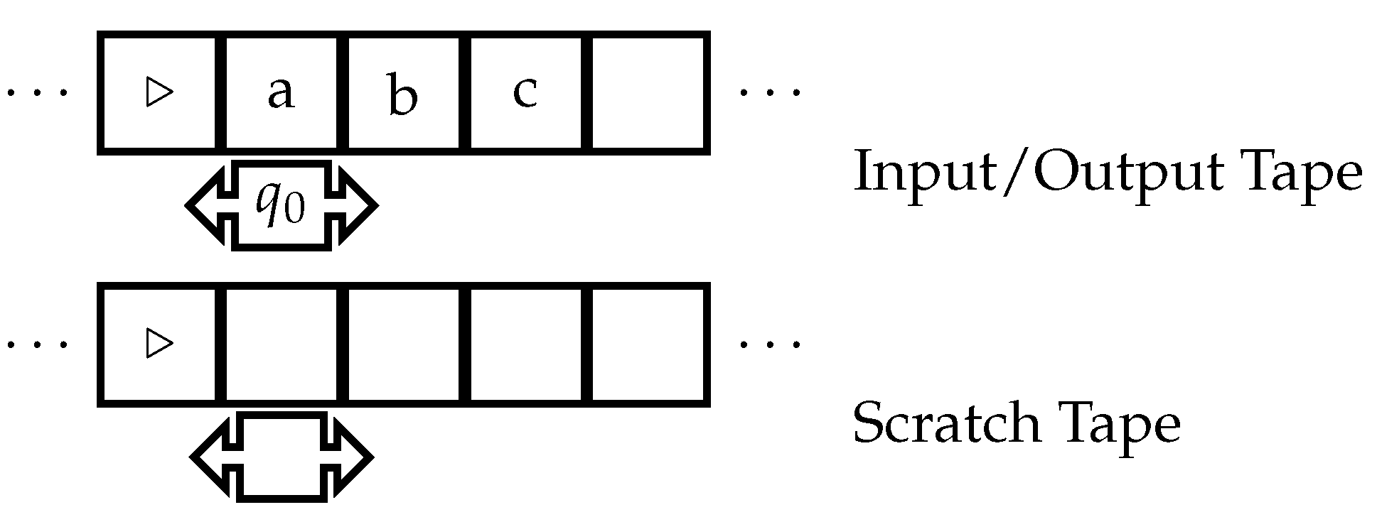
Figure 2. A Single Symbol Time-Traveling Turing Machine (SSTTM) sending a symbol back in time.

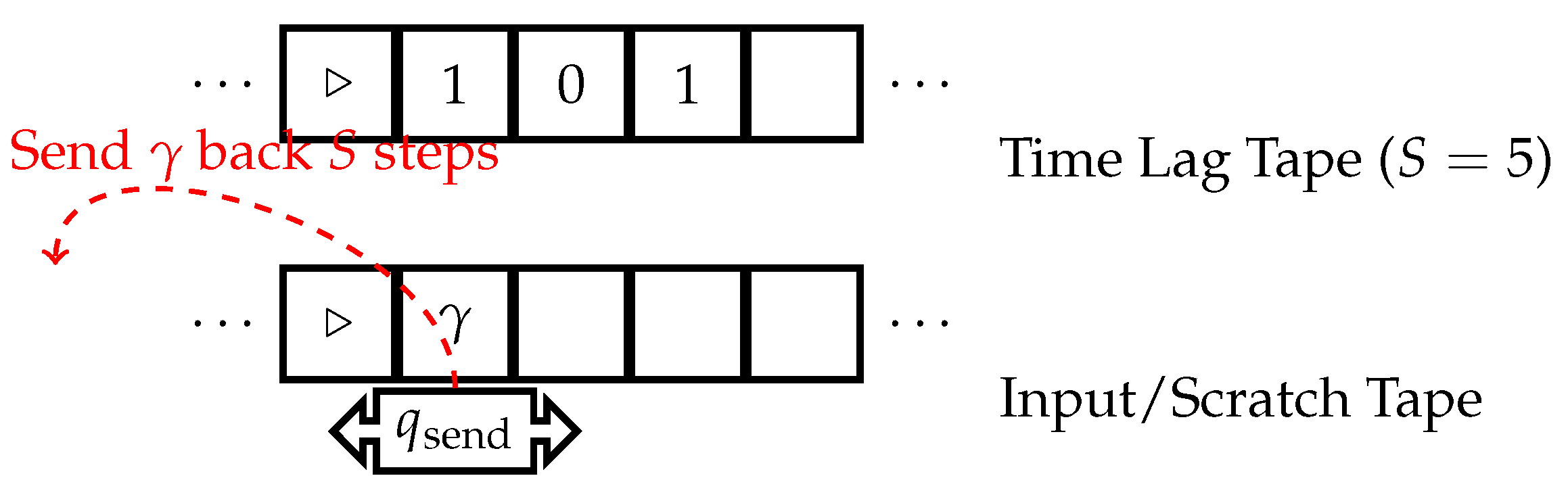
Figure 3. An Internal Clock Time-Traveling Turing Machine (ICTTM) sending a symbol to time 0.

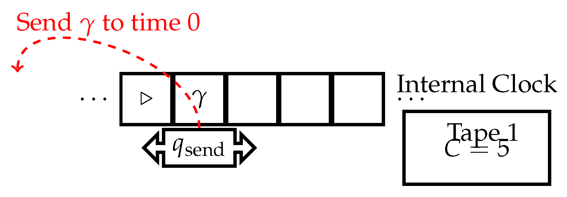
Figure 4. A Full Tape Internal Clock Time-Traveling Turing Machine sending the entire non-blank contents of tape 1 to time 0.

Disclaimer/Publisher’s Note: The statements, opinions and data contained in all publications are solely those of the individual author(s) and contributor(s) and not of MDPI and/or the editor(s). MDPI and/or the editor(s) disclaim responsibility for any injury to people or property resulting from any ideas, methods, instructions or products referred to in the content.

© 2024 by the authors. Licensee MDPI, Basel, Switzerland. This article is an open access article distributed under the terms and conditions of the Creative Commons Attribution (CC BY) license (http://creativecommons.org/licenses/by/4.0/).

Copyright: This open access article is published under a Creative Commons CC BY 4.0 license, which permit the free download, distribution, and reuse, provided that the author and preprint are cited in any reuse.

MDPI Initiatives

Important Links

Choose an area of interest and we will send you notifications of new preprints at your preferred frequency.

Disclaimer

Time-travelling Turing Machines and the Self-consistent Halting Problem

Abstract

1. Introduction

2. Related Work

3. Definitions

3.1. Traditional Turing Machines

3.2. Single Symbol Time-Traveling Turing Machine

3.3. Internal Clock Time-Traveling Turing Machine

3.4. Full Tape ICTTM

4. Properties

4.1. Self-Consistent Computability

4.2. Complexity Constraints

5. Conclusions

Acknowledgments

References

MDPI Initiatives

Important Links

Subscribe