Submitted:
30 May 2024
Posted:
30 May 2024
You are already at the latest version
Abstract
To enhance the performance of visual SLAM in underwater environments, this paper presents an enhanced front-end method based on visual feature enhancement. The method comprises three modules aimed at optimizing and improving the matching capability of visual features from different perspectives. Firstly, to address issues related to insufficient underwater illumination and uneven distribution of artificial light sources, a brightness consistency recovery method is pro-posed. This method employs an adaptive histogram equalization algorithm to balance the brightness of images. Secondly, a method for denoising underwater suspended particulates is introduced to filter out noise from the images. After image-level processing, a combined underwater acousto-optic feature association method is proposed, which associates acoustic features from sonar with visual features, thereby providing distance information for the visual features. Finally, utilizing the AFRL dataset, the improved system incorporating the proposed enhancement methods is evaluated for performance against the OKVIS framework. The system achieves better trajectory estimation accuracy compared to OKVIS and demonstrates robustness in underwater environments.
Keywords:
underwater SLAM
; underwater image processing
; visual feature point enhancement
; association of acoustic and visual feature
1. Introduction
Exploration of underwater environments has been severely constrained by harsh conditions and limited perception [1]. The utilization of robot-assisted technology for underwater exploration can alleviate the cognitive burden on divers and enhance work efficiency. Improving the robot’s capacity to perceive the surrounding environment can significantly broaden the diver’s field of vision, while the diversity and redundancy in information acquisition can offer more effective assistance for diver decision-making [2]. In recent years, numerous camera-based SLAM frameworks have emerged, capable of generating reliable state estimation results in both indoor and outdoor settings [3]. However, these frameworks are predominantly designed for terrestrial environments and lack consideration for underwater applications, resulting in suboptimal performance when deployed in underwater settings [4].
In underwater environments, the uneven attenuation of natural light within water results in color deviation and contrast degradation in images. Scenes lacking natural light are often illuminated using artificial light sources, which, being single-point light sources with limited power, cast numerous shadows in irregular underwater environments. Additionally, regardless of the lighting method used, suspended substances in the water cause diffuse reflection, disrupting the normal propagation of light [5]. These conditions render cameras more susceptible to factors such as limited visibility, color absorption, fogging, and fluctuations in light intensity when capturing underwater images, leading to image blurring compared to terrestrial shooting conditions [6]. Consequently, the application of optical cameras reliant on visual information is restricted in underwater environments [6]. As a result, when utilizing a vision-based state estimation system with continuous images captured underwater, various adverse factors mentioned above can significantly impact the extraction of stable feature points for motion estimation from feature matching. This may lead to the generation of numerous anomalous feature points due to various noise disturbances, ultimately resulting in decreased estimation accuracy or tracking failure [7].
To enhance the feasibility of visual odometry in underwater environments, this paper proposes an improved VIO front-end method based on visual feature enhancement. The main contributions are as follows:
1. Image-Level Enhancements: The proposed method integrates image brightness enhancement and suspended particulate removal techniques. This significantly increases the probability of successful detection of visual feature points after application.
2. Geometric Feature Association: From a spatial geometry perspective, a feature association method that integrates sonar acoustic features with visual features is proposed, enabling visual features to obtain depth information.
3. Benchmarking with AFRL Dataset: A comparative analysis is conducted using the AFRL dataset against the classical OKVIS visual SLAM framework. This tests the limitations of traditional frameworks in underwater datasets and demonstrates the feasibility of the proposed method.
2. Related Work
In recent years, significant strides have been made in developing image-based visual state estimation algorithms, thanks to the relentless efforts of researchers. These algorithms are applicable for state estimation using data from monocular, binocular, and RGBD cameras [8], and they exhibit commendable performance in both indoor and outdoor settings. Within the visual odometry (VO) framework, ORB-SLAM [9] stands out for its capability to extract feature points across different images. By matching and tracking these feature points over time, ORB-SLAM computes changes in their positions, enabling the derivation of the camera’s motion trajectory and attitude relative to the features. In contrast, the LSD-SLAM [10] algorithm does not rely on traditional feature point extraction. Instead, it directly utilizes grayscale information from images to perform depth estimation and motion tracking. This approach yields dense feature and depth information, thereby enhancing map density while preserving local feature details.
However, owing to the specific characteristics of underwater environments, conventional visual SLAM methods cannot be readily adapted for underwater use. Visual odometry systems are notably sensitive to fluctuations in lighting conditions, and the uneven absorption of light in underwater environments can markedly impede the extraction and matching of feature points by the feature checker. In scenarios where water depth surpasses 30 meters, natural light becomes nearly non-existent, prompting the necessity of employing active lighting methods [11] for underwater optical imaging systems. Ancuti [12] introduced a systematic processing method for enhancing underwater images, rooted in the principle of minimizing information loss to improve color and visibility. They proposed a dark channel a priori algorithm, which mitigates the influence of the red channel while accounting for the effects of optical radiation absorption and scattering on image degradation, thereby enhancing the visual quality of the image. Similarly, Barris [13] proposed a light propagation model based on visual quality perception. Building upon existing physical models, they integrated the physics of light propagation to mitigate the impact of optical radiation attenuation, further enhancing the quality of underwater images.
Water in natural environments frequently harbors a substantial quantity of suspended matter, encompassing sediments, sand, and dust particles produced by diverse planktonic organisms. The irregular morphology and surface roughness of these suspended objects pose challenges in maintaining consistent observations, as the perceived information varies with viewing angles [14]. Consequently, image fidelity diminishes, contours become indistinct, and the signal-to-noise ratio declines. These suspended materials can be considered noise in image feature extraction, significantly impacting the extraction, matching, and tracking of visual feature points in images. As a result, the operational efficiency of underwater feature-point-based visual odometry is markedly reduced compared to on-ground scenarios. Therefore, it is essential to filter underwater suspended particles from images.
The null domain denoising method partially mitigates noise by eliminating components at specific frequencies. Nonetheless, when noise in underwater images and their structural texture intersect in the frequency domain, it results in blurred image texture and unclear edges. This issue can be addressed by a nonlinear median filter enhanced through the weighted median method. Linear filters in the wavelet domain are exemplified by the Wiener filter [15]. However, the degradation process of the actual signal may not conform to a Gaussian distribution, rendering this type of filter potentially detrimental to the visual quality of the denoised image. Celebi [16] introduced a wavelet domain spatially adaptive Wiener filter image denoising algorithm to enhance the visual quality of the image post noise reduction. Additionally, C. J. Prabhakar [17] proposed an adaptive wavelet band thresholding method for reducing noise in underwater images. This method aims to filter out additive noises in the image, including scattering and absorption effects, as well as suspended particles visible to the naked eye, resulting from sand and dust on the seabed.
In recent years, there has been a growing focus on the study of vision-based multi-sensor fusion SLAM systems in underwater environments. The ORB-SLAM system demonstrated successful application in a lake characterized by clear water quality and favorable lighting conditions, yielding promising results [18]. Additionally, Hogue proposed an underwater robot state estimation algorithm grounded in multi-state constrained Kalman filtering. This algorithm incorporates pressure sensor information alongside the fusion of camera and IMU data, enabling direct acquisition of water depth data. The integration aims to enhance system estimation accuracy along the vertical orientation [19]. Furthermore, the SVIN [20] system, an extension of OKVIS, integrates sonar detection information into the VIO system to introduce additional constraints for position estimation, thereby enhancing the stability of position estimation. However, there are few papers that discuss the comprehensive optimization of underwater SLAM systems by integrating both image processing and utilizing distance sensor sonar information. This is also the primary focus of the present paper.
3. System Overview
In this paper, the existing VIO framework is used as the basis for pre-processing the camera images. The paper continues to utilize the visual feature extraction methods, the IMU-integrated VIO front-end framework, and the back-end BA optimization method from the framework. The key improvements of this paper focus on the visual image processing at the front end and the integration of sonar measurement information. Labeling the camera coordinate system, the IMU coordinate system, the sonar coordinate system, and the world coordinate system as , with the state vector denoted as , the bit position denoted using the quaternion , the linear velocity as , the bias of the gyroscope as , and the bias of the accelerometer as , and all the variables denoted in the world coordinate system, the state of the system can be denoted as :
The overall flow of the system is depicted in the system block diagram. Initially, data from each sensor undergoes preprocessing to yield the camera image, the IMU pre-integration term, and the position information of the sonar features. The original images are processed through brightness recovery and suspended matter removal modules, followed by the extraction and matching of visual feature points. The IMU data is used to correct aberrations caused by motion during the sonar scanning cycle. Next, sonar features are matched with camera features, and the distance information from sonar detection is utilized to refine the depth estimation of camera feature points. The sonar feature information corresponding to the camera features is then used to enhance the accuracy of the camera features on the image plane, thereby reducing the reprojection error. Finally, a joint error optimization is conducted, incorporating the reprojection error of the camera features, IMU error, and sonar distance error, to estimate feature points and the robot’s state.
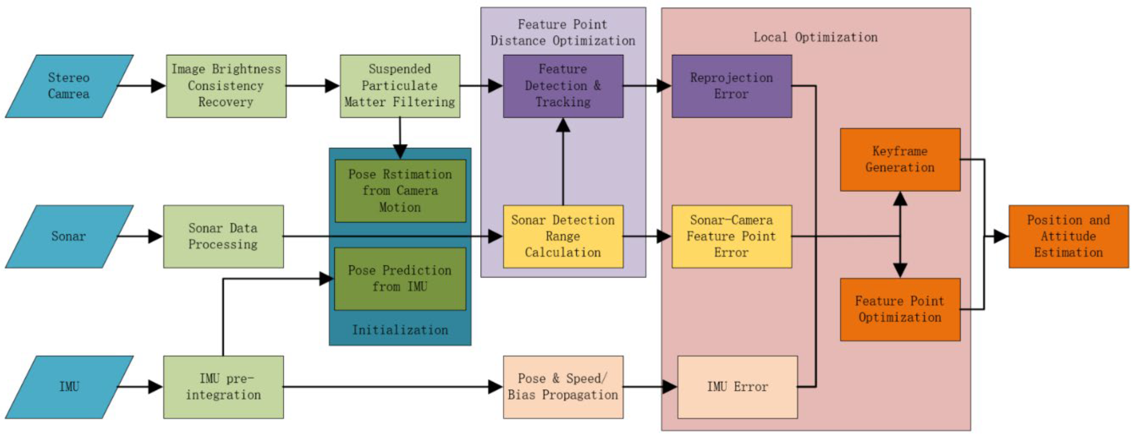
Figure 1.
System Architecture Diagram.
3. Proposed Method
3.1. Underwater Image Brightness Consistency Recovery
Visual odometry is more sensitive to changes in light, and the uneven absorption of light in the water body will greatly affect the extraction and matching of feature points by the feature checker. Different wavelengths of light in the water have different attenuation characteristics, in the visible range, the longer wavelengths of red light in the water has a larger attenuation rate, the weakest penetration rate, usually only 3-4 meters, and blue light, green light and other shorter wavelengths of light can be propagated in the water for a longer distance, the uneven attenuation of this light will lead to underwater optical image distortion, usually manifested as the image of the bluish, greenish. This color distortion will lead to a reduction in image contrast and increase the difficulty of feature point extraction.
In the underwater cave environment, the main source of light is the searchlight carried by the exploration platform, which is an artificial light source with strong directionality, limited by the power of the light source, the brightness difference between the inside and outside of the artificial light source illumination range is large. The use of searchlights in the illumination of the designated target, but also because of the light path of the mask blocking, resulting in more shadow areas. These influences are manifested in the image as an uneven distribution of brightness, i.e., the image is roughly characterized by high brightness in the central area and low brightness in the surrounding area. And part of the protruding object back to the light source is a low brightness black area.
To improve the contrast of underwater images, image contrast enhancement processing is usually performed using the HE (histogram equalization) method. However, in use, if the algorithm is used directly to process underwater images, it will appear to increase the brightness of high-brightness regions and decrease the brightness of low-brightness regions, thus exacerbating the overexposure and underexposure of the image. In order to reduce the occurrence of such situations, it is necessary to restore the light intensity of the underwater image before image enhancement to reduce the brightness differences in the image regions caused by uneven illumination of the artificial light source.
To establish an underwater light model, the image information recorded by the camera is regarded as the superposition of the reflected light in the scene and the scattered light in the water, and the light intensity at each position in the image can be expressed as the following equation:
Where represents the light intensity of the image at the position, the gray value of the image at that position. is the reflected light intensity at the location, is the scattered light intensity, and is the component weight. Due to the limitation of the irradiation range of the artificial light source resulting in different light intensity at different locations, the light range attenuation coefficient is introduced to represent the attenuation coefficient at the image location .
The maximum value of the mean gray value of the pixel points in the coverage range of each window is selected as the base brightness, and the range attenuation coefficient at this position is considered to be 1. According to the invariance of the light distribution, the mean and the standard deviation of the pixel distribution of each window should be roughly the same in the case of sufficient light. Therefore, the light attenuation coefficients at different positions can be obtained from the difference of each window .
Since the range of the window is small, it can be approximated that the scattered light intensity within the range of is unchanged, at any position within the window, the scattered light intensity is constant, so the variance can be deduced as the following equation:
where is the variance of the reflected light distribution in window and is the mean of the reflected light in that window. Find the maximum value of the standard deviation after removing the effect of the attenuation coefficient in all windows, denoted as .
Approximating the weight of the scattered light at this position as 0, i.e.,, based on the standard deviation invariance assumption , the weight of the receivable reflected light satisfies the following equation:
In the absence of natural light interference, the minimum value of the reflected light pixel gray value in each window is close to 0:
under these conditions:
where denotes the minimum value of the light intensity of the image in window . So the light attenuation coefficient at each position in the image can be expressed as:
Based on the attenuation coefficient and the scaling coefficient , the pixel can be calculated:
After performing the necessary calculations on the pixel points, it is possible to restore the image pixel values to reflect conditions of uniform and sufficient lighting. This approach helps to mitigate the problem of insufficient contrast enhancement caused by uneven illumination to a certain extent.
Then, the underwater images are processed using an adaptive histogram equalization (AHE) algorithm based on illumination consistency reduction. Initially, the images are divided into numerous small regions, and each region undergoes histogram equalization (HE) tailored to its local characteristics. For darker regions, the brightness is increased to enhance contrast and visual effect, while for brighter regions, the brightness is reduced to prevent overexposure or distortion.
Figure 2 presents the results of the original image, HE processed image, and AHE processed image. It is evident that the image directly processed by HE exhibits a larger area of overexposure and white noise. This occurs because the HE algorithm processes the entire image globally, directly adjusting the gray level distribution across the entire image. When higher brightness areas exist in the original image, enhancing the overall contrast results in the brightness values of these highlighted areas being further amplified, leading to overexposure and noise. Conversely, for darker regions, the gray levels are reduced, diminishing the contrast of useful information, which leads to the loss of some fine image details and a reduction in the number of feature points. In contrast, after AHE processing, the contrast near the rock surface is improved, and the contours of objects in the distant background become clearer. Compared with using the HE algorithm directly, AHE avoids the problems of brightness anomalies and white noise caused by global histogram equalization.
Histograms are often utilized to infer the quality of an image. An image that includes all possible gray levels and has uniformly distributed gray levels across its pixel values is characterized by high contrast and varied gray tones. Consequently, if the gray values of an image are randomly distributed, its histogram should ideally resemble a normal distribution. In the case of the HE processed image, the corresponding histogram exhibits a trend resembling a normal distribution. However, the presence of an unusually large number of pixels with certain gray levels, which are transitionally broadened during the equalization process, leads to the appearance of spikes in the histogram. These spikes indicate the presence of noise or specific textures and details in the image, reflecting the limitations of global histogram equalization in handling diverse image regions uniformly. For the AHE processed image, the histogram distribution is closer to a normal distribution compared to the original image. The peaks of the gray values of the pixels are also reduced to a certain extent, indicating that the brightness uniformity processing has been effective. This improvement helps avoid issues of excessive brightness values in local areas of the image, resulting in a more balanced and visually coherent image. The enhancement provided by AHE thus effectively mitigates the problems associated with global histogram equalization, such as overexposure and noise, while preserving fine image details and improving overall feature detection.
3.2. B. Underwater Suspended Particulate Filtration
Image blurring caused by underwater suspended particulate matter is induced by irregular tiny particles floating in the load-bearing object, similar to the image blurring caused by haze conditions on the ground. Therefore, the suspended matter in the water can be regarded as a kind of noise and processed using an image defogging algorithm. The underwater environment is complex and dynamic. Even within the same body of water, variations in factors such as season, water temperature, and light conditions can affect the quality of images captured by the camera. Consequently, it is essential to determine the necessity of filtering suspended particulate matter based on specific image conditions. The presence of suspended particulate matter introduces a gray haze, which can be identified through blurring detection techniques.
By detecting the image gradient, the degree of blurring in an image can be assessed. The image gradient is calculated by determining the rate of change along the x-axis and y-axis of the image, thereby obtaining the relative changes in these axes. In image processing, the gradient of an image can be approximated as the difference between neighboring pixels, using the following equation:
A Laplacian operator with rotational invariance can be used as a filter template for computing the partial derivatives of the gradient. The Laplacian operator is defined as the inner product of the first-order derivatives of the two directions, denoted as :
In a two-dimensional function, the second-order differences in the x and y directions are:
The equation is expressed in discrete form to be applicable in digital image processing
If the pixels have high variance, the image exhibits a wide frequency response range, indicating a normal, accurately focused image. Conversely, if the pixels have low variance, the image has a narrower frequency response range, suggesting a limited number of edges. Therefore, the average gradient, which represents the sharpness and texture variation of the image, is used as a measure: a larger average gradient corresponds to a sharper image. Abnormal images are detected by setting an appropriate threshold value to determine the acceptable range of sharpness. When the calculated result falls below the threshold, the image is considered blurred, indicating that the concentration of suspended particulate matter is unacceptable and requires particulate matter filtering. If the result exceeds the threshold, the image is deemed to be within the acceptable range of clarity, allowing for the next step of image processing to proceed directly.
The issue of blurring in underwater camera images resulting from suspended particulate matter can be addressed by drawing parallels with haze conditions on the ground. Viewing suspended particulate matter in water as a form of noise, an image defogging algorithm (DCP) can be employed to mitigate the blurring effect.
It is hypothesized that in a clear image devoid of suspended particulate matter, certain pixels within non-water regions, such as rocks, consistently exhibit very low intensity values:
Dark channels in underwater images stem from three primary sources: shadows cast by elements within the underwater environment, such as aquatic organisms and rocks; brightly colored objects or surfaces, like aquatic plants and fish; and darkly colored objects or surfaces, such as rocks. Hence, the blurring observed in these images can be likened to the occlusion experienced in haze-induced scenarios. Consequently, suspended particulate matter can be regarded as noise and filtered accordingly.
Before applying the DCP method to filter suspended particles from underwater images, it is crucial to acknowledge a significant disparity between underwater images and foggy images. The selective absorption of light by the water body results in a reduced red component in the image, which can potentially interfere with the selection of the dark channel. To effectively extract the dark channel of the underwater image, the influence of the red channel must be mitigated. Therefore, the blue-green channel is selected for dark channel extraction.
The imaging model of foggy image is expressed as
where is the image to be de-fogged, is the fog-free image to be recovered, the parameter A is the optical component, which is a constant value in Eq. and is the transmittance. The two sides of the equation are deformed by assuming that the transmittance is constant within each window and defining it as , and then two minimum operations are performed on both sides to obtain the following equation
The imaging model of the image with the presence of more suspended particulate matter is expressed as:
Where denotes each channel of the color image, denotes a window centered on pixel , denotes the R, G and B color channels. Since imaging is different from foggy day imaging, in order to avoid the uneven attenuation of light interfering with the selection of the dark channel, it is necessary to exclude the influence of the red channel and select only the blue-green channel for dark channel extraction.
According to the dark primary color theory, the intensity of the dark channel of the fog-free image tends to zero. It means the intensity of the dark channel in the fogged image is greater than that of fog-free image. Because in foggy environments, the light is subjected to scattering by particles, which results in additional light, and the intensity of the fogged image is higher than that of the fog-free image.
and it can be deduced that:
The intensity of the dark channel of a fogged image is used to approximate the concentration of fog, which is expressed as the density of suspended particulate matter in the underwater image. Considering the situation in the actual underwater environment, retaining a certain degree of suspended particulate matter, the transmissivity can be recorded as:
For each pixel the minimum value in the color channel component is deposited into a grayscale image of the same size, and then this grayscale image is minimum filtered. However, in some cases, extreme values of the transmittance can occur. In order to prevent the value from being abnormally large when the value is very small, leading to the overall overexposure of the image screen, a threshold value is set, and the final image recovery formula is as follows:
The defogging algorithm proves effective in reducing noise and halo effects. As depicted in Figure 3, it is evident that post-processing with the dark-channel priority algorithm enhances object details and sharpens object edges, thereby improving clarity.
3.3. Acoustic and Visual Feature Association for Depth Recovery
The demanding underwater conditions pose significant challenges to the extraction and tracking of visual feature points, resulting in a noticeable degradation in the accuracy of depth direction information estimation. Leveraging the precise distance information provided by the sonar, the camera’s feature scale can be effectively recovered. This study enhances the feature extraction capability through image-level processing and subsequently utilizes sonar distance data to further augment the matching proficiency of feature points.
The sonar’s spatial detection range is typically visualized as a spherical configuration with the sonar device at its center. When targeting a specific direction, this detection process effectively confines the search area to a prism-shaped region. Leveraging the sonar’s horizontal resolution, individual beams are associated with a fan-shaped ring in cross-section, facilitating target range determination. As a result, the sizing of these fan-shaped rings serves as a criterion for filtering candidate matches between the sonar and camera feature points.
The uncertainty linked to sonar detection range escalates in tandem with the separation between targets. As targets move farther away, a single sonar beam encompasses a broader expanse, especially evident in the vertical dimension where the aperture of the sonar beam widens. In earlier processing approaches, a common practice involved extracting the point with the highest bin value within a beam and then calculating the spatial distance to its centroid, deemed as the spatial feature point for the sonar. However, the uncertainty linked to sonar features stems from two key factors. Firstly, the sparse resolution of sonar, coupled with the influence of the underwater environment on the distortion of bin values, hampers the accurate reflection of the true distance to targets. Secondly, as one moves away from the center of the sonar, a bin value corresponds to a spatial region rather than a precise point, as illustrated in Figure 4.
Therefore, accurately correlating sonar feature points with visual feature points is challenging, and this paper explores an alternative approach. Firstly, the spatial position of a coarse visual feature point is calculated. Then, for each beam, the maximum bin value is identified. In the sequence, the two values before and after this maximum bin value are also considered, totaling five bin values. A joint spatial region is constructed from the geometry of these five bin values within the sonar’s beam structure. Any feature points falling within this region are considered the candidates to be mutually correlated with the corresponding sonar feature point, as shown in Figure 5.
Typically, the distribution of feature points in an image exhibits strong randomness, with local areas containing more edges and corners, resulting in a higher concentration of extracted feature points. To enhance computational efficiency, a quadtree method is commonly employed to achieve a uniform distribution of feature points. Traditional quadtree homogenization involves recursively partitioning the feature points in the image into four equally divided regions. The recursion terminates based on a predetermined condition related to the number of feature points in the image. Ultimately, only one feature point is retained in each final segmented region after equalization.
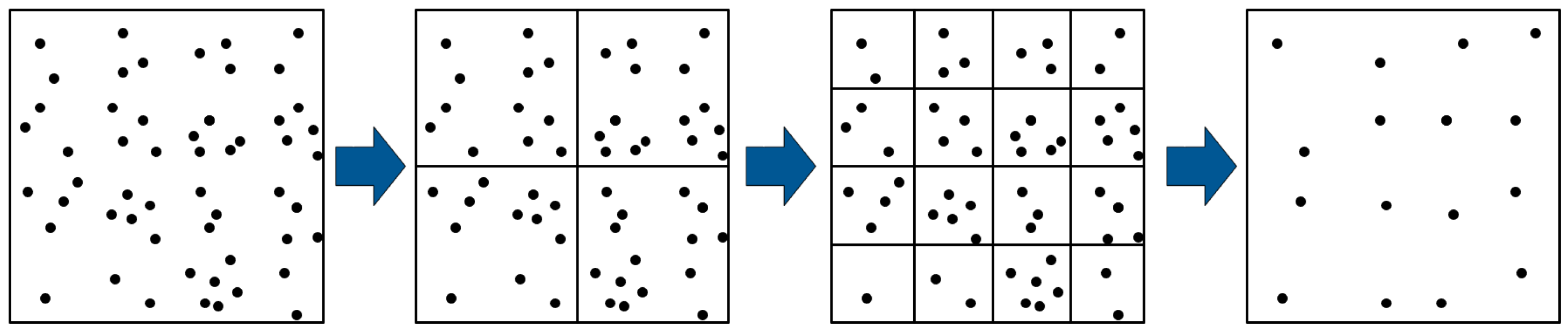
Figure 6.
Using Quadtree for features unification.
After undergoing the aforementioned association method, the visual features associated with a single sonar feature may be one or multiple. In the case of multiple visual features, these visual features may span across multiple image regions after quadtree segmentation. During the partitioning process, when a group of mutually correlated points are connected to form a polygon, the quadtree’s partitioning region for this group of points should be larger than its Minimum Bounding Rectangle (MBR). As shown in Figure 7, In the partitioning process shown in the bottom-left corner, although it ensures that each small area contains visual feature points, the visual feature points associated with a sonar feature are divided into different child node regions. However, as shown in the top-right corner, one node’s region contains the entire set of points.
In traditional quadtrees only leaf nodes can be assigned object (one polygon), hence an object may be assigned to more than one leaf node,it means these leaf nodes share same depth from sonar feature. While in the proposed quadtree segmentation, if the range matrix of a node contains the MBR of an indexed object and the range matrices of its four child nodes do not contain the MBR of that indexed object (intersecting or diverging), the object is added to that node. In this way, the root node intermediate nodes are able to be assigned indexed objects and the objects assigned to each node are not duplicated.
The termination condition for quadtree recursion in this method does not solely rely on the number of feature points but must also consider the resolution capabilities of the sonar. By incorporating the detection distance and resolution of the sonar, the maximum detection range of its sonar opening can be calculated. When the size of the divided area in the quadtree becomes smaller than the area of the polygenes, simple image segmentation becomes ineffective in providing optimal information for feature matching between the sonar and the camera. Thus, image segmentation is terminated to conserve computational resources.
3. Results and Experiments
The system proposed in this paper for underwater SLAM will undergo testing utilizing an AFRL dataset [21], which encompasses a binocular camera, an inertial measurement unit, a sonar, and a water pressure sensor. The specific sensor model is as follows.:
- Two IDS UI-3251LE cameras,
- IMAGENEX 831L Sonar,
- Microstrain 3DM-GX4-15 IMU,
- Bluerobotics Bar30 pressure sensor.
The two cameras are synchronized in hardware via an Arduino board, capturing 15 frames per second at a resolution of 1600x1400 pixels. The sonar scans the plane with an angular resolution of 0.9°, with a maximum effective detection distance of 6 meters and a scanning period of 4 seconds. The effective range of the sonar detection beam intensity values is between 6 and 255. The IMU provides angular velocity and acceleration data at a frequency of 100Hz. The depth sensor measures depth at a frequency of 15Hz. All acquired and processed data are recorded in a package file using ROS. The detailed ROS topics for the sensor are as shown in Table 1. The dataset was collected from a cave in Ginnie Spring, Florida, USA. The sonar was configured with a higher rate to accommodate the underwater environmental scene. As natural lighting was lacking in the cave, an underwater searchlight was utilized to supplement the scene during video recording. However, due to constraints related to the searchlight’s light angle and power, it could only illuminate within a certain angle corresponding to the direction of the underwater robot’s travel. This led to significant differences in illumination between the center and edge areas, resulting in poorer camera light conditions compared to shallow water environments. In this dataset, the presence of dynamic obstacles such as fish and crabs, coupled with substantial amounts of suspended particulate matter in the underwater environment, will significantly affect both acoustic signal-based sonar and optical-based underwater cameras.
Firstly, feature extraction is tested using a feature detector to extract SIFT features from the original image and the processed image, which employed adaptive histogram equalization (AHE) combine with dark channel priority (DCP) suspension removal algorithm, comparing the image before and after processing. The experiment first tested four different scenarios, corresponding to subfigures in Figure 8 below. From the comparison, it can be seen that the processed images successfully extracted more feature points and distributed them more uniformly.
To further quantify the comparison results directly, the experiment counted the number of feature points extracted from four sets of images. As shown in Table 2, it’s clear that the number of feature points goes up after using the HE algorithm, which is the first method discussed in this paper. Especially for the fourth image, which has a greenish tint and looks blurry. After applying both the AHE and suspension removal algorithms together, meaning the first and second image processing methods combined, it’s obvious that even more feature points are extracted.
Next, the matching capability of the visual feature points in the processed images was tested. In the matching process, the red connecting line represents that the pair of matching has higher confidence while the green connecting line represents that the pair of matching has lower confidence. It can be observed that after processing, in all four scenes, the majority of feature point matches maintained a high level of confidence.
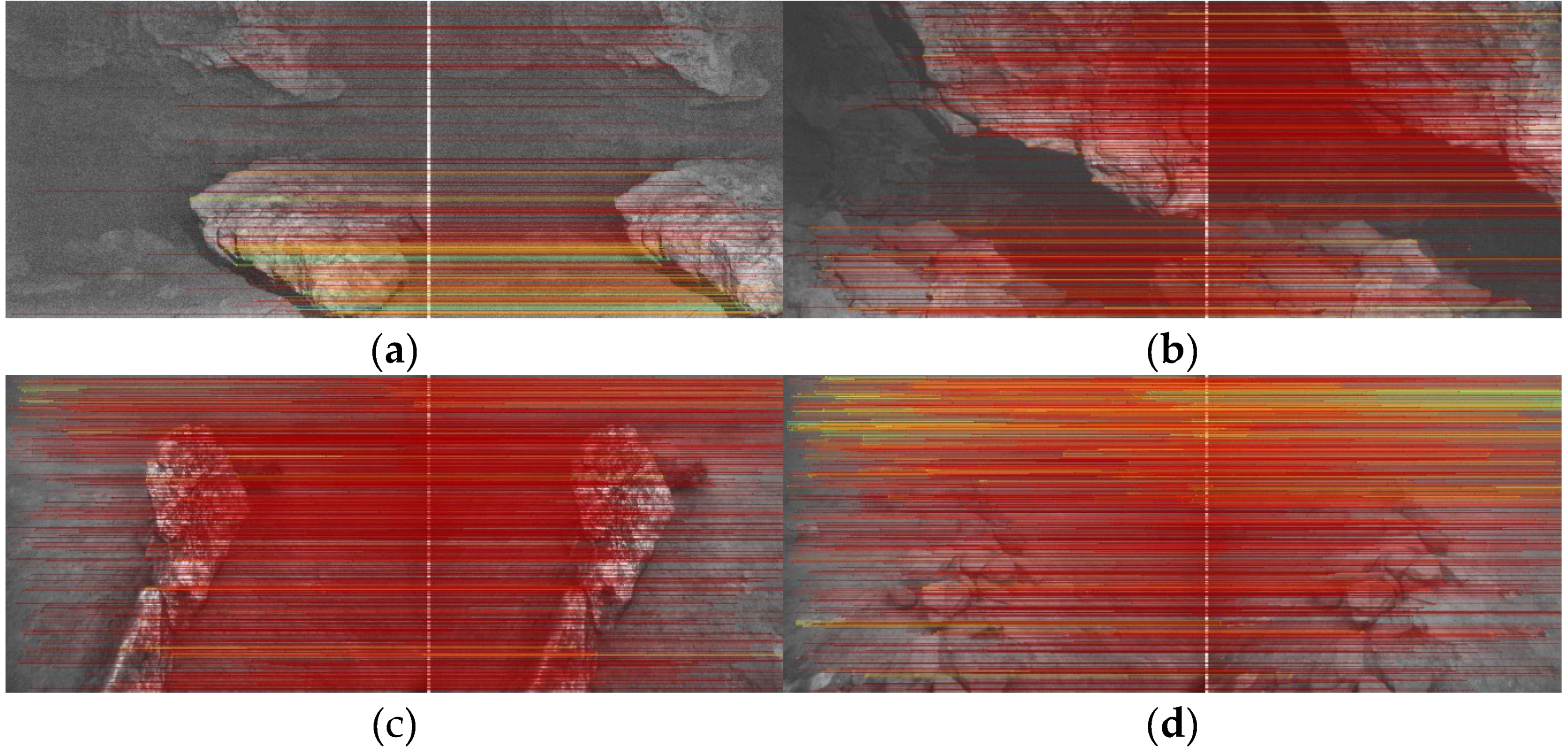
Figure 9.
Test of visual feature points matching for processed images.
To quantitatively evaluate the performance of the proposed method, this paper conducted statistical comparisons between the number of matched feature points in the original, unprocessed images and the processed ones, as shown in Table 3.
In Scene 1, feature points primarily cluster in the exposed rocky areas above and to the lower right of the image, resembling ground scenes. However, there exists a shadowed area beneath the rock where direct light cannot reach, resulting in lower confidence levels for feature point matching near this shadowed region. Consequently, such areas appear as lightly colored matches in the image. The background area at the far end is also constrained by the searchlight’s power, resulting in the area appearing black and rendering feature extraction impossible. Nevertheless, the overall quantity and quality of matches meet the system’s basic requirements. In scene 2, the primary concentration of feature points also lies within the upper right and lower left exposed rock areas. The shadowed area within the camera’s view is reduced, and appropriate illumination contributes to high confidence levels in the feature points. The only region in this image lacking sufficient brightness for feature extraction and matching is the crevice area between the rocks, attributable to inadequate illumination. In Scene 3, feature points are not only present on the rock surface but also in certain areas of the seabed, facilitating feature extraction. And the method proposed in this paper can still further increase the number of feature point matches based on this foundation. In scene 4, the surfaces of the rocks are covered with flocculent graded sediment, which may hinder the efficiency of relying on corner points and edges for feature extraction. This is reflected in the lower confidence level of feature matching in the upper half of the image. In the original, unprocessed image, there were even no successful matches of any feature point pairs. However, after the image enhancement process, it is still able to successfully match the features.
Comparing the number of feature point matches before and after image enhancement reveals that more matches can be obtained from the enhanced image compared to the original ones. In the first, second, and third images, where feature extraction is feasible in the original image, the enhanced image demonstrates varying degrees of improvement in the number of feature matches where the successfully matching feature pairs increase. The primary significance of image processing lies in enhancing the system’s robustness in coping with underwater extremes, a prominently demonstrated in the fourth image. In the fourth image, the contrast is most apparent. In the original image, the absence of feature matches, indicated by a count of zero, is attributed to the low number of extracted features and the challenge of finding their counterparts in the other image. However, following the image enhancement process, the number of extracted features can be restored to normal levels.
As OKVIS visual SLAM framework is utilized for ARFL data evaluation, this paper enhanced front-end processing by integrating three proposed functional modules, thus reconstructing the front-end accordingly of OKVIS. The resulting system, termed the “improved system,” was comprehensively compared with OKVIS results and ground truth in Figure 10. In the trajectory plots, the dashed line represents the ground truth, the blue trajectory depicts the path generated by the improved system, and the green trajectory represents OKVIS’s path. Observation reveals that the blue trajectory closely aligns with the reference trajectory, whereas the green trajectory exhibits numerous cumulative errors and considerable fluctuations.
On the x-axis, the difference between the two methods is minimal, but the trajectory of the improved system exhibits smoother motion compared to OKVIS, which demonstrates more fluctuations. This trend is also noticeable along the y-axis, particularly in the middle section. In terms of the z-axis direction, the OKVIS trajectory exhibits significant errors in the middle and front sections, with substantial drift evident towards the tail end. Conversely, the improved system consistently maintains a high level of alignment with the ground truth, demonstrating remarkable consistency throughout. Next, statistical analysis and presentation of trajectory errors were performed using the EVO plugin, the results are shown from Figure 11 and Table 4.
Based on the Figures and tables provided, the results obtained from the improved method outperform those of the OKVIS run comprehensively. In terms of both maximum and average error metrics, the improved method consistently maintains values below 1 when compared to the ground truth. Conversely, the OKVIS results exhibit larger errors, with the maximum error reaching 2.5, indicating significant trajectory shifts in certain instances. Additionally, the sum of squared errors surpasses 50 for OKVIS, suggesting highly unstable trajectories characterized by increased fluctuations and significant drift towards the tail section.
5. Conclusions
OKVIS is a well-established VIO (Visual-Inertial Odometry) visual SLAM framework. However, our data testing indicates that directly applying this framework to underwater environments does not yield effective results. The primary factor affecting accuracy is the insufficient number of visual feature points extracted and successfully matched in underwater images, which significantly degrades estimation accuracy, particularly in the vertical direction. This issue arises because underwater robots may experience jitter or rapid lens switching during ascent and descent, reducing the already limited number of matches and potentially causing misalignment.
Conversely, the enhanced system, after processing in image enhancing and feature association between camera and sonar, demonstrated commendable performance on the test dataset. It maintained strong consistency with the ground truth trajectory and exhibited robust performance, with no significant fluctuations throughout the trajectory. Experimental results suggest that the underwater visual SLAM system, augmented with image enhancement and distance sensor assistance, has shown substantial performance improvements. Nevertheless, future research will aim to determine whether the image enhancement method demonstrates good generalization performance in bright water areas and whether the segmented association method can effectively enhance system performance across different positions of sonar beams.
Author Contributions
The paper provide by seven authors, the authors contributions as follows: Conceptualization, Haiyang Qiu; Data curation, Yijie Tang; Funding acquisition, Haiyang Qiu, Hui Wang; Methodology, Yijie Tang and Lei Wang; Project administration, Haiyang Qiu; Software, Yijie Tang; Supervision, Hui Wang,Lei Wnag; Writing – original draft, Yijie Tang; Writing – review & editing, Dan Xiang and MingMing Xiao. All authors have read and agreed to the published version of the manuscript.
Funding
This work was supported by the National Natural Science Foundation of China (52101358, 41906154), Jiangsu Provincial Key Research and Development Program So-cial Development Project (BE2022783), and the Zhenjiang Key Research and Devel-opment Plan (So-cial Development) Project, No. SH2022013.
Acknowledgments
Authors would like to gratitude any reviewers who have made comments on this article
Conflicts of Interest
The authors declare no conflicts of interest.
References
- Liu H, Zhang G, Bao H. A survey of monocular simultaneous localization and mapping. Journal of Computer-Aided Design & Computer Graphics, 2016.
- Davison A J, Reid I D, Molton N D, et al. MonoSLAM: Real-time single camera SLAM. IEEE transactions on pattern analysis and machine intelligence, 2007; Volume 29, pp. 1052-1067. [CrossRef]
- B. Triggs, P. McLauchlan, R. Hartley, and A. Fitzgibbon. bundle adjustment - a modern synthesis. in W. Triggs, A. Zisserman, and R. Szeliski, editors, Vision Algorithms: Theory and Practice, 2000; Volume 1883 of LNCS, pp. 298-372.
- F. Dellaert and M. Kaess. Square Root SAM: Simultaneous localization and mapping via square root information smoothing. Int.J. of Robotics Research,2006; Volume 25, pp. 1181-1203. [CrossRef]
- M. Kaess, H. Johannsson, R. Roberts, V. Ila, J. J. Leonard, and F. Dellaert. iSAM2: Incremental smoothing and mapping using the Bayes tree. Int. J. of Robotics Research, 2012; Volume 31, pp. 217-236. [CrossRef]
- A. Agarwal, K. Mierle, and Others. Ceres solver. http://ceres-solver.org.
- R. Kummerle, G. Grisetti, H. Strasdat, K. Konolige, and W. Burgard. g2o: A general framework for graph optimization. In IEEE Int. Conf. on Robotics and Automation (ICRA), Shanghai, China, May 2011.
- Y. Bar-Shalom, X. R. Li, and T. Kirubarajan. Estimation with Applications to Tracking and Navigation. John Wiley and Sons, 2001.
- G. P. Huang, A. I. Mourikis, and S. I. Roumeliotis. Observability-based rules for designing consistent EKF SLAM estimators. Int. J. of Robotics Research, 2010; Volume 29, pp. 502-528. [CrossRef]
- D. Scaramuzza and F. Fraundorfer. visual odometry [tutorial]. Part I: The first 30 years and fundamentals. IEEE Robotics Automation Magazine, 2011; Volume 18, pp. 80 -92.
- Klein G, Murray D. Parallel tracking and mapping for small ar workspaces. 2007 6th IEEE and ACM international symposium on mixed and augmented reality, 2007; pp. 225-234.
- Mur-Artal R, Tardos J D. ORB-SLAM2: an Open-Source SLAM System for Monocular, Stereo and RGB-D Cameras. 2016. [CrossRef]
- Campos C, Elvira R, JJG Rodríguez, et al. ORB-SLAM3: An Accurate Open-Source Library for Visual, Visual-Inertial and Multi-Map SLAM. 2020. [CrossRef]
- M. A. Fischler and R. C. Bolles. Random sample consensus: a paradigm for model fitting with applications to image analysis and automated cartography. Commun.ACM, 1981; Volume 24, pp. 381-395.
- K. MacTavish and T. D. Barfoot. at all costs: a comparison of robust cost functions for camera correspondence outliers. in Conf. on Computer and Robot Vision, 2015.
- M. Irani and P. Anandan. all about direct methods. in Proc. Workshop Vis. Algorithms: Theory Pract, 1999; pp. 267-277.
- Kerl C, Sturm J, Cremers D. Dense visual slam for rgb-d cameras. 2013 IEEE/RSJ International Conference on Intelligent Robots and Systems, 2013; pp. 2100-2106.
- Engel J, Schops T, Cremers D. Lsd-slam: Large-scale direct monocular slam. European conference on computer vision, 2014; pp. 834-849.
- Gao X, Wang R, Demmel N, et al. Ldso: Direct sparse odometry with loop closure. International Conference on Intelligent Robots and Systems, 2018; pp. 2198-2204.
- Forster C, Zhang Z, Gassner M, et al. SVO: Semidirect Visual Odometry for Monocular and Multicamera Systems. IEEE Transactions on Robotics, 2017; Volume 33, pp. 249-265. [CrossRef]
- Rosten E. Machine learning for high-speed corner detection. European Conference on Computer Vision. Springer-Verlag, 2006.
- Lucas B D, Kanade T. An Iterative Image Registration Technique with an Application toStereo Vision. Proceedings of the $7^th$ International Joint Conference on Artificial Intelligence. Morgan Kaufmann Publishers Inc. 1997.
- Paul, L, Rosin. Measuring Corner Properties. Computer Vision & Image Understanding, 1999.
- Muja M. Fast approximate nearest neighbors with automatic algorithm configuration. Proc Vissapp, 2009.
- Burri, M, Nikolic J, Gohl P, Schneider T, Rehder J, Omari S, Achtelik M W. and Siegwart R. The EuRoC micro aerial vehicle datasets. International Journal of Robotics Research, 2016; Volume 35, pp. 1157-1163. [CrossRef]
Figure 2.
Gray-scale image, HE-processed image, illuminance-consistent AHE-processed image and corresponding histograms.
Figure 2.
Gray-scale image, HE-processed image, illuminance-consistent AHE-processed image and corresponding histograms.
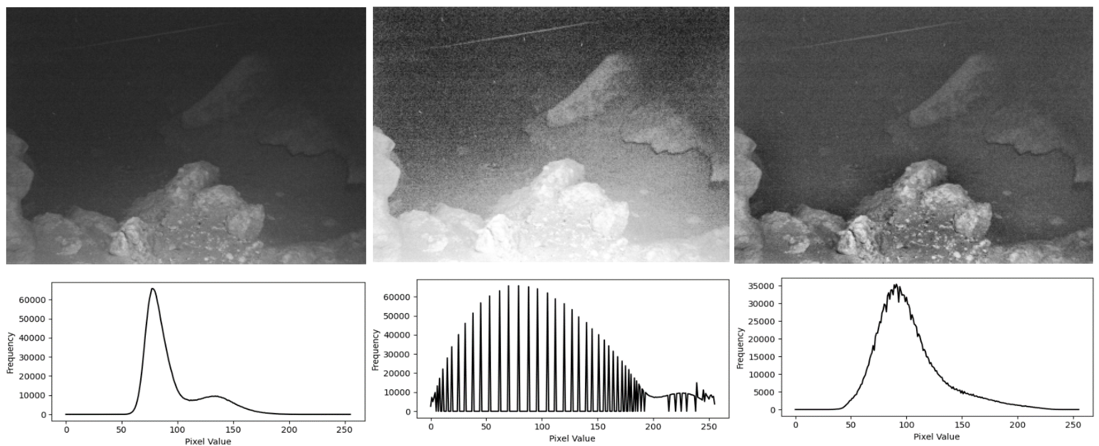
Figure 3.
Original image and processed image using DCP.
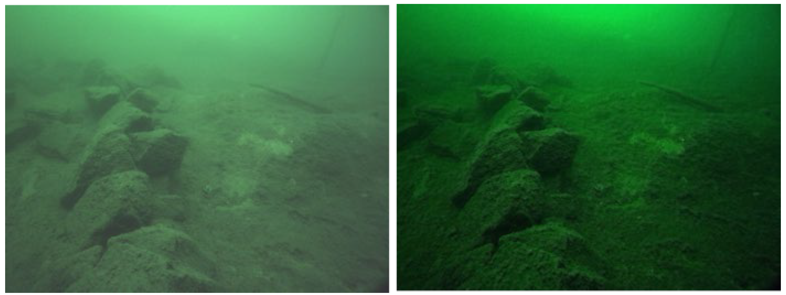
Figure 4.
Beam coverage increases with distance and may cover many feature points.
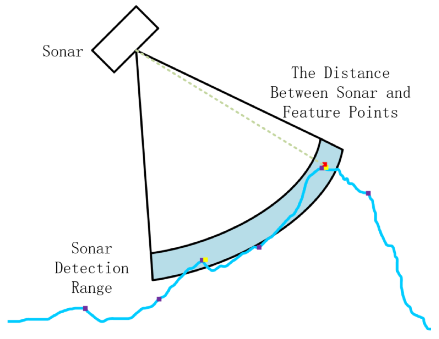
Figure 5.
Candidates matching of visual feature points with one sonar feature point.
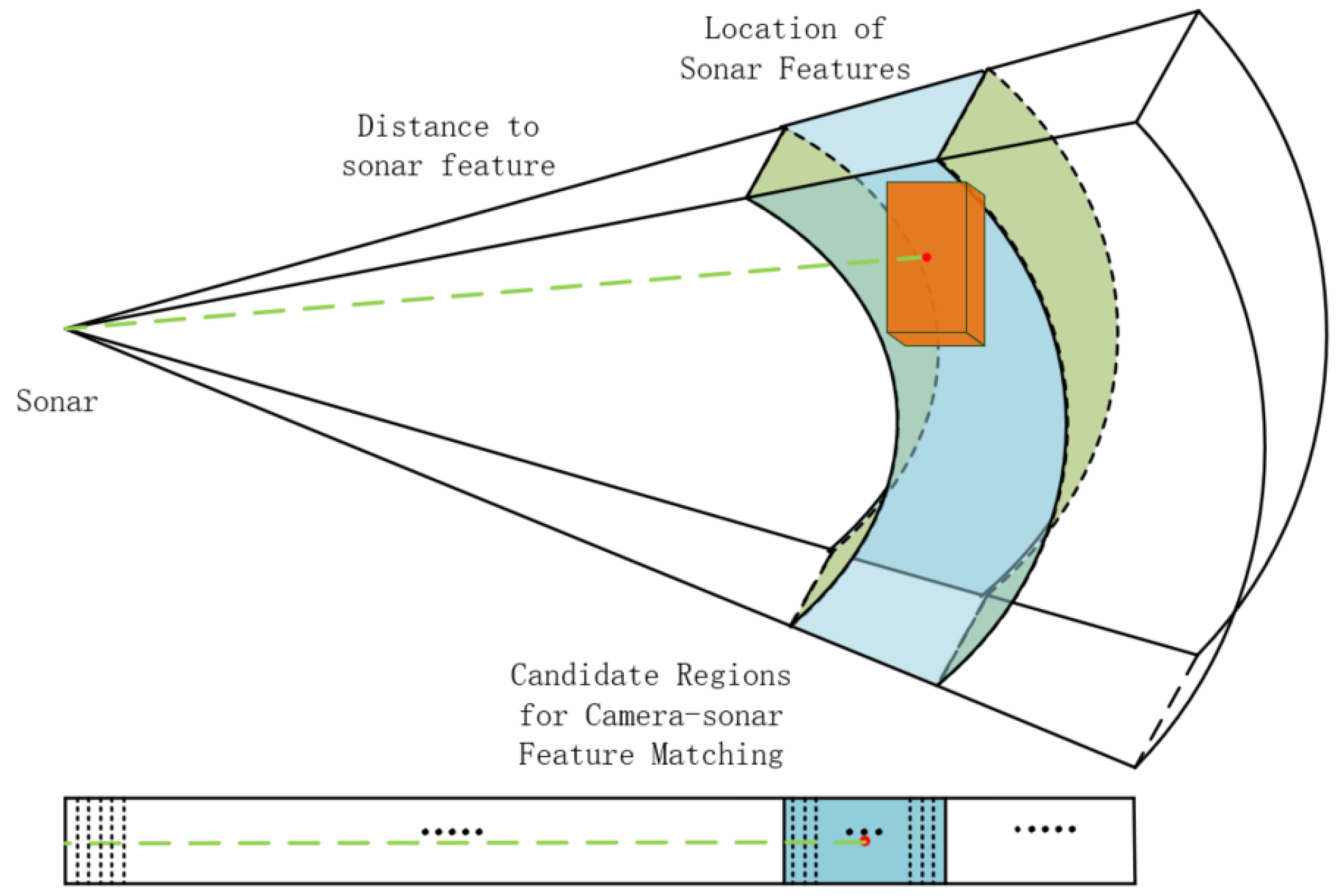
Figure 7.
Different polygenes in partitions of quadtree.
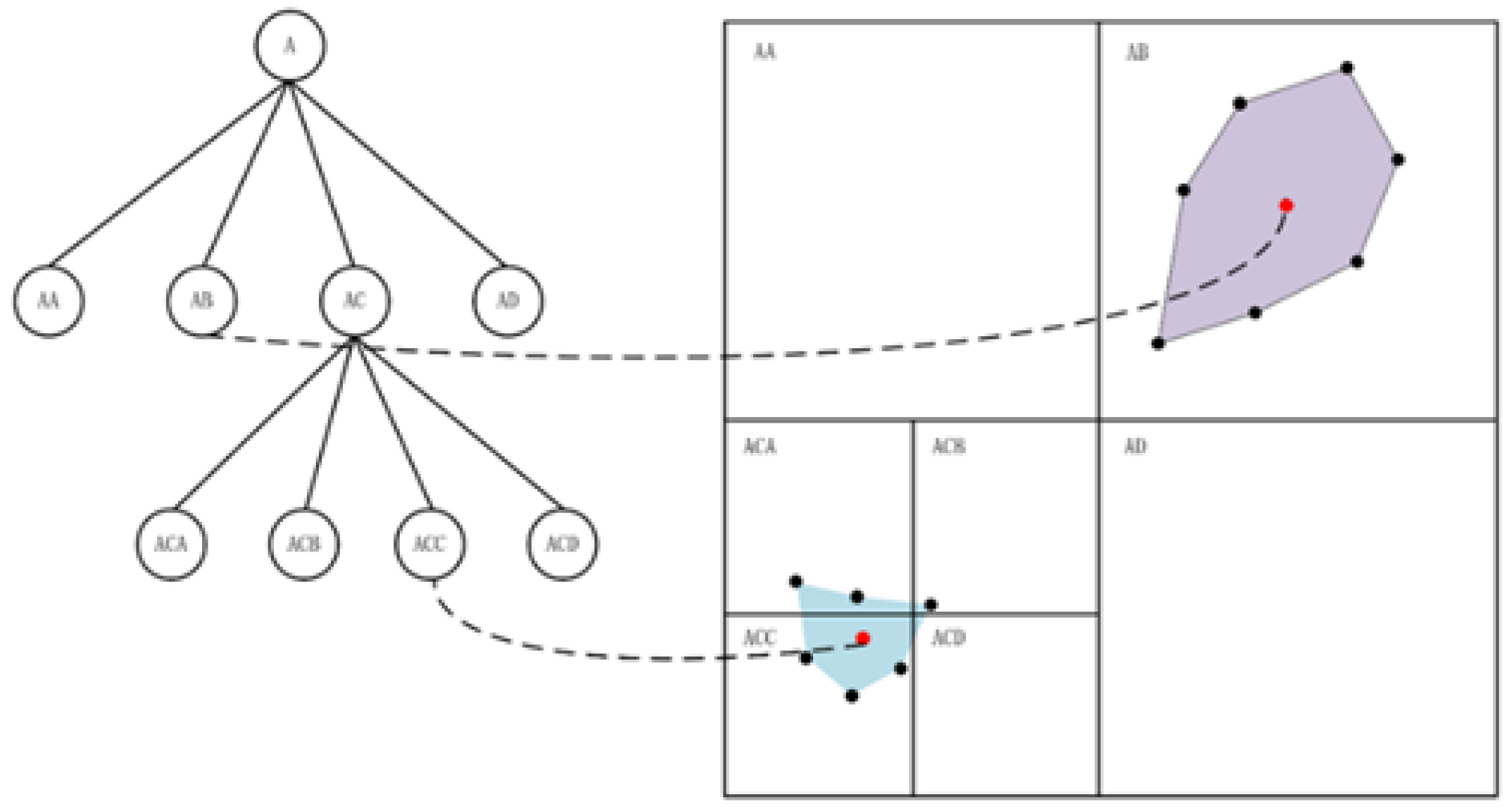
Figure 8.
Visual feature points extraction contrast in different scenarios.
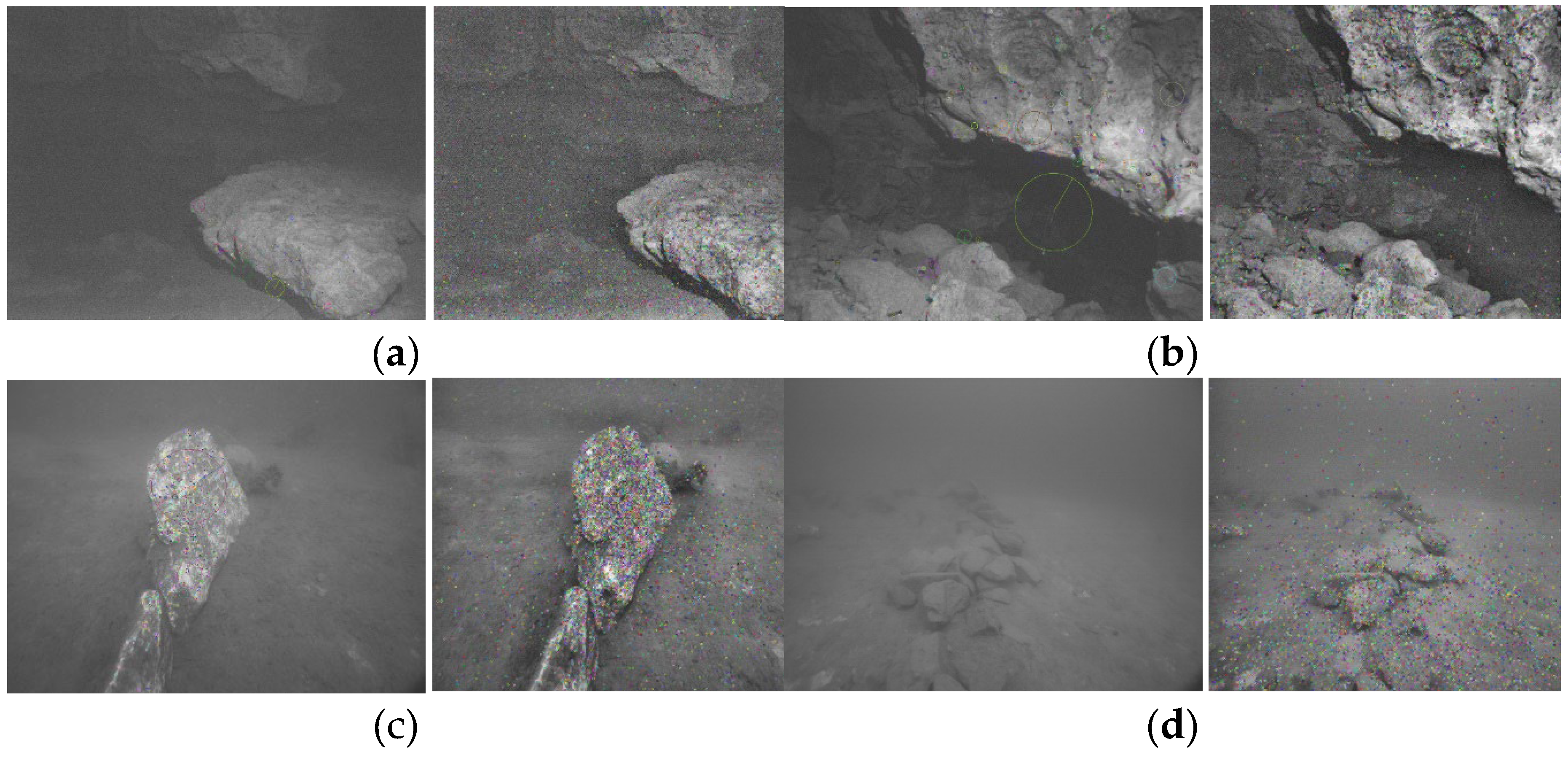
Figure 10.
Trajectory Plot of the Dataset (a) Comparison of trajectories for OKVIS, our work and ground truth; (b) Local amplification of three axes.
Figure 10.
Trajectory Plot of the Dataset (a) Comparison of trajectories for OKVIS, our work and ground truth; (b) Local amplification of three axes.
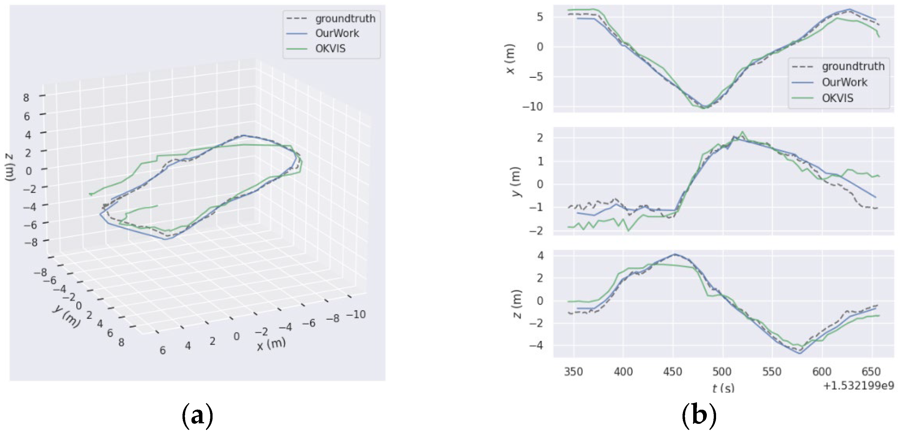
Figure 11.
Display of absolute trajectory error using EVO (a) Absolute trajectory error (APE) between the improved method and ground truth; (b) Display of APE statistics for improved method compared with ground truth (c) APE between OKVIS and ground truth (d) Display of APE statistics for OKVIS compared with ground truth.
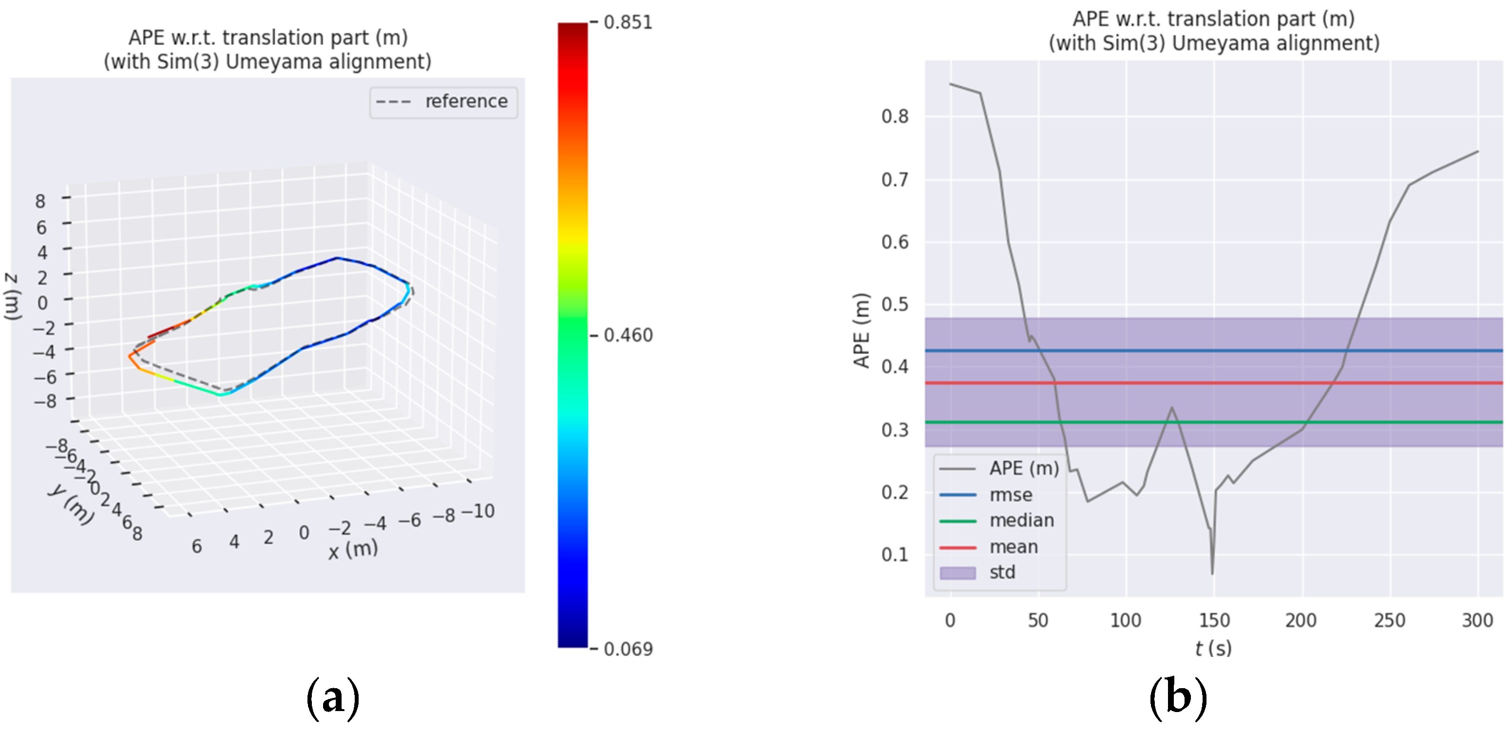
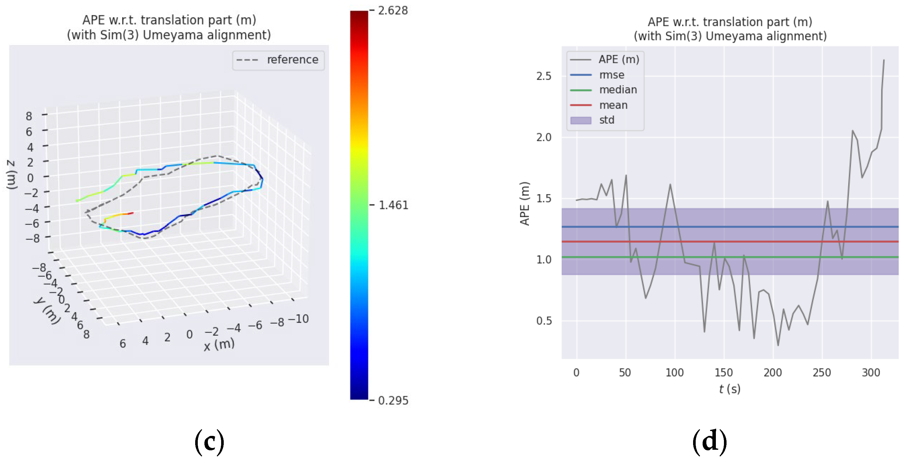

Table 1.
Topic information of different sensors in the dataset.
| Sensor | Ros topic | Data |
|---|---|---|
| Camera | /slave1/image_raw/compressed | Left camera image |
| /slave2/image_raw/compressed | Right camera image | |
| IMU | /imu/imu | Angular velocity and acceleration data |
| Sonar | /imagenex831l/range_raw | Acoustic image |
| Pressure sensor | /bar30/depth | Bathymetric data |
Table 2.
Comparison of the number of feature points before and after image processing.
| 1 | 2 | 3 | 4 | |
| Original Image | 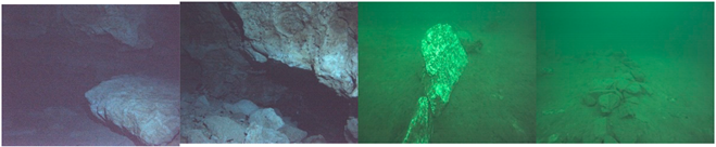 |
|||
| 103 | 351 | 806 | 2 | |
| HE Image | 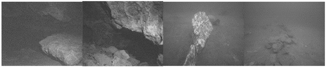 |
|||
| 135 | 460 | 821 | 288 | |
| Improving AHE+ Suspended Matter Removal | 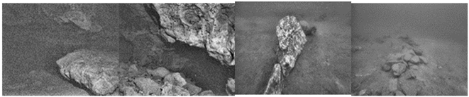 |
|||
| 198 | 682 | 1125 | 523 | |
Table 3.
Numbers of successfully matching pairs for different scenes.
| 1 | 2 | 3 | 4 | |
|---|---|---|---|---|
| Original Image | 85 | 321 | 613 | 0 |
| Enhanced Image | 125 | 456 | 746 | 233 |
Table 4.
This is a table. Tables should be placed in the main text near to the first time they are cited.
Table 4.
This is a table. Tables should be placed in the main text near to the first time they are cited.
| The improved system results compared with groundtruth | OKVIS results compared with groundtruth | |
|---|---|---|
| max | 0.829411 | 2.627724 |
| mean | 0.366091 | 1.148321 |
| median | 0.309184 | 1.020354 |
| min | 0.077178 | 0.295083 |
| rmse | 0.420158 | 1.267575 |
| sse | 7.414390 | 93.191309 |
| std | 0.206181 | 0.536756 |
Disclaimer/Publisher’s Note: The statements, opinions and data contained in all publications are solely those of the individual author(s) and contributor(s) and not of MDPI and/or the editor(s). MDPI and/or the editor(s) disclaim responsibility for any injury to people or property resulting from any ideas, methods, instructions or products referred to in the content. |
© 2024 by the authors. Licensee MDPI, Basel, Switzerland. This article is an open access article distributed under the terms and conditions of the Creative Commons Attribution (CC BY) license (http://creativecommons.org/licenses/by/4.0/).
Copyright: This open access article is published under a Creative Commons CC BY 4.0 license, which permit the free download, distribution, and reuse, provided that the author and preprint are cited in any reuse.


