

Submitted:
23 May 2024
Posted:
23 May 2024
You are already at the latest version
Abstract
Autonomous search is an ongoing cycle of sensing, statistical estimation and motion control with objective to find and localise targets in a designated search area. Traditionally, the theoretical framework for autonomous search combines the sequential Bayesian estimation with the information theoretic motion control. This paper formulates autonomous search in the framework of possibility theory. Although the possibilistic formulation is slightly more involved than the traditional, it provides means for quantitative modelling and reasoning in the presence of epistemic uncertainty. This feature is demonstrated in the paper in the context of partially known probability of detection, expressed as an interval value. The paper presents an elegant Bayes-like solution to sequential estimation, with the reward function for motion control defined to take into account the epistemic uncertainty. The advantages of the proposed search algorithm are demonstrated by numerical simulations.
Keywords:
Possibility theory
; autonomous systems
; robust estimation
1. Introduction
Search is a repetitive cycle of sensing, estimation (localisation) and motion control, with objective to find and localise one, or as many as possible targets, inside the search volume, in the shortest possible time. The searching platform (agent) is assumed to be mobile and capable of sensing, while the detection process is typically imperfect [1], in the sense that the probability of detection is less than one, with a small (but non-negligible) probability of false alarms. Autonomous search refers to the search by an intelligent agent without human intervention.
Search techniques have been used in many situations. Examples include: rescue and recovery operations, security operations (e.g., search for toxic or radioactive emissions), understanding animal behaviour, military operations e.g., (anti-submarine warfare) [2]. Search techniques have also been increasingly important in field robotics [3,4,5,6] for the purpose of carrying out dirty and dangerous missions. A formal search theory has roots in the works by Koopman [7], and has since expanded and extended to different problems and application. It can be categorised into a static versus a moving target search, a reactive versus a non-reactive target search, a single versus multiple target search, a cooperative versus a non-cooperative target search, etc [2].
In this paper we focus on an area search for an unknown number of static targets using a realistic sensor on a single searching platform, conceptually similar to the problems discussed in [8,9,10]. The searching agent can be a drone, equipped with a sensor capable of detecting targets on the ground with a certain probability of detection (as a function of range) as well with some false alarm probability.
The dominant theoretical framework for the formulation of search is probability theory, where Bayesian inference is used to update sequentially the posterior probability distribution of target locations, as the new measurements are collected over time [9,11,12,13,14]. Sensor motion control is typically formulated as a partially observed Markov decision process (POMDP) [15]. The information state in the POMDP formulation is represented by the posterior probability distribution of targets. The set of sensor motion controls (actions), which determine where the searching agent should move next, can be made by a single or multiple steps ahead. The reward function in POMDP maps the set of admissible actions to a set of positive real numbers (rewards) and is typically formulated as a measure of information gain (e.g., the reduction of entropy, Fisher information gain) [16].
Statistical inference is based on mathematical models. In the target search context, we need a model of sensing, which incorporates the uncertainty with regards to the probability of true and false detection as well as the statistics of target (positional) measurement errors. This uncertainty in the Bayesian framework is expressed by probability functions - in particular, the probability of detection, the probability of false alarm, and the probability density function (PDF) of a positional measurement, given the true target location. The key limitation of the Bayesian approach, however, is that these probabilistic models must be known precisely. Unfortunately, in many practical situations it is difficult or even impossible to postulate the precise probabilistic models. Consider for example the probability of detection. It typically depends on the (unknown) size and reflective characteristics of the target, and hence at best can be specified as a confidence interval (rather than a precise probability value), for a given distance to the target. Thus we need to deal with epistemic uncertainty, which incorporates both randomness and partial ignorance.
In order to deal with epistemic uncertainty, an alternative mathematical framework for inference is required. These theories involve non-additive probabilities [17] for the representation and processing of uncertain information. They include, for example, possibility theory [18], Dempster-Shafer theory [19] and imprecise probability theory [20]. Because the last two theories are fairly complicated, and at present applicable only to discrete state spaces, we focus on possibility theory [21,22]. Recent research in nonlinear filtering and target tracking [23,24,25,26,27] have demonstrated that possibility theory provides an effective tool for uncertain knowledge representation and reasoning.
The main contributions of this paper include a theoretical formulation of autonomous search in the framework of possibility theory and a demonstration of its robustness in the presence of epistemic detection uncertainty. The paper presents an elegant Bayes-like solution to sequential estimation, with a definition of the reward function for motion control which take into account the epistemic uncertainty. Evaluation of the proposed search algorithm considers the scenarios with a large number of targets and for two cases for the probability of detection as a function of range: (i) the case when is known precisely; (ii) the case when is known only as an interval value.
The paper is organised as follows. Section 2 introduces the autonomous search problem. Section 3 reviews the standard probabilistic formulation of autonomous search and presents the theoretical framework for estimation using possibility functions. Section 4 formulates the new possibilistic solution to autonomous search. Numerical results with comparison are presented in Section 5, while the conclusions are drawn in Section 6.
2. Problem Formulation
Consider a search area . A surveillance drone, flying at a fixed altitude, has a mission to autonomously search and localise the ground-based static targets in , as in [10]. The number and locations of targets are unknown. Following [9,10], the search area is discretized into cells of equal size. The presence or absence of a target in the nth cell at a discrete-time can be modelled by a Bernoulli random variable (r.v.) , where by convention denotes that a target is present, (i.e., 0 denotes target absence) and is the cell index.
Suppose the search agent is equipped with a sensor (e.g., a radar), which illuminates a region at time k and collects a set of detections within . Each detection reports the Cartesian coordinates of a possible target. However, the sensing process is uncertain in two ways: (1) the reported target coordinates are affected by measurement noise; (2) the measurement set may include false detections and also may miss some of the true target detections. The probability of true target detection is a (monotonically decreasing) function of range and is specified as an interval value for a given range.
The objective is to detect and localise as many targets as possible in the shortest possible time.
3. Background
3.1. Probabilistic Search
Autonomous search in the Bayesian probabilistic framework is typically information driven. The information state at time k is represented by the posterior probability of target presence in each cell of the discretised search area. This posterior probability at time k is denoted by , where is the sequence of measurement sets up to the current time k. The posterior probability of target absence is then simply , and therefore is unnecessary to compute.
The target or threat map is defined as the array . Initially, at time , the map is specified as , for all , thus expressing the initial ignorance. As time progresses and the search agent collects measurements, the threat map is sequentially updated using Bayes’ rule. Consequently, the information content of the threat map is increasing with time. The information content of the threat map is measured by its entropy, defined as
Note that at , and that entropy decreases with time.
In order to explain how the threat map is updated using Bayes’ rule, let us introduce another Bernoulli r.v. , where represents the event that a detection from the set has fallen inside the nth cell ( represents the opposite event). Bayes’ rule is given by:
where the subscript is temporarily removed from and in order to simplify the notation, and .
Note that and represent the probability of detection and the probability of false alarm, respectively. Then and .
Given , if none of the detections in falls into the nth cell, the probability is updated according to (2) as
where is the probability of detection and is the probability of false-alarm, in the nth cell of search area at time k.
After collecting the measurement set , the searching agent must decide on its subsequent action, that is, where to move (and sense) next. Suppose the set of possible actions (for movement) is . This set can be formed by considering one or more motion steps ahead (in the future). The reward function associated with every action is typically defined as the reduction in entropy of the threat map [10], that is:
Note that the expectation operator with respect to the (future) detection set . In practical implementation, in order to simplify computation, we typically adopt an approximation that circumvents in (5). This approximation involves the assumption that a single realisation for is sufficient: the one which results in hypothetical detection(s) at those cells which are characterised by a high probability of target presence, i.e., such that , where is a threshold close to 1. The searching agent chooses the action which maximises the reward, i.e.,:
3.2. The Possibilistic Estimation Framework
Possibility theory is developed for quantitative modelling of epistemic uncertainty. The concept of uncertain variablein possibility theory, plays the same role as the random variable in probability theory. The main difference is that the quantity of interest is not random, but simply unknown, and our aim is to infer its true value, out of a set of possible values. The theoretical basis of this approach can be found in [28,29,30]. Briefly, uncertain variable is a function , where is the sample space and is the state space (the space where the quantity of interest lives). Our current knowledge about X can be encoded in a function , such that is the possibility (credibility) for the event . Function is not a density function, it is referred to as a possibility function, being the primitive object of possibility theory [22]. It can be viewed as a membership function determining the fuzzy restrictions of minimal specificity (in the sense that any hypothesis not known to be impossible cannot be ruled out) about x[18]. Normalization of is , if is uncountable, and , if is countable.
In the formulation of the search problem, we will deal with two binary uncertain variables, corresponding to r.v.’s and . Hence, let us focus on a discrete uncertain variable X and its state space . The possibility measure of an event is a mapping , where is the set of all subsets of . Mapping satisfies three axioms: (1) ; (2) , and (3) the possibility of a union of disjoint events and is given by . Possibility measure is related to the possibility function as follows:
for every . There is also a notion of necessity of an event , which is dual to in the sense that:
where is the complement of A in . One can interpret the necessity-possibility interval as the belief interval, specified by the lower and upper probabilities in the sense of Wiley [20]. Note that for a binary variable , this interval can be expressed for event as , where, due to normalisation, the following condition must be satisfied: .
4. Theoretical Formulation of Possibilistic Search
4.1. Information State
The information state at time k in the framework of possibility theory will be represented by two posteriors:
- the posterior possibility of target presence , and
- the posterior probability of target absence .
We need both of them, because cannot be worked out from . Consequently, during the search, two posterior possibility maps need to be updated sequentially over time, and , where .
Suppose now that the probability of detection is specified by an interval value, that is
where and represent the lower and upper probability of this interval, respectively. Because detection event is a binary variable, due to reachability constraint for probability intervals [33], (9) implies that the probability of non-detection is in interval . Then, via normalisation we can express the possibility of detection and the possibility of non-detection (in cell n at time k) as1:
satisfying . Interval represents the necessity-possibility interval for the probability of detection.
In general, the probability of detection by a sensor, as well as the two possibilities and , are typically dependent on the distance between the nth grid cell and the searching agent position at time k.
In a similar manner we can also assume that the probability of false alarm is specified by an interval value, that is , where and represent the possibility of no false alarm and the possibility of false alarm (in cell n at time k), respectively.
Next we explain how to sequentially update, during the search, the two posterior possibility maps, (for target presence) and (for target absence). The proposed update equations follow from (3) and (4), when we apply the Bayes-like update rule (8).
Given and detection set , if none of the dectections in falls into the nth cell, the possibility of target presence in the nth cell is updated as follows:
for . Similarly, in this case is updated according to:
If a detection from falls into the nth cell, then the update equation for can be expressed as:
And finally, in this case the update equation for is given by:
Note that the probability of target presence in each cell of the search area, using the described possibilistic approach, is expressed by a necessity-possibility interval, i.e.,
for , where . Initially, at time (before any sensing action), the posterior possibility maps are set to:
meaning that , for . This is an expression of initial ignorance about the probability of target presence in the nth cell.
4.2. Epistemic Reward
Let us first quantify the amount of uncertainty contained in the information state, represented by two posterior possibility maps, and . Various uncertainty (and information) measures in the context of non-additive probabilistic frameworks have been proposed in the past [35,36,37]. We adopt the principle that epistemic uncertainty, on the continuous state space, corresponds to the volume under the possibility function [25,37]. For a possibility function over a discrete state space , epistemic uncertainty equals the sum . The possibilistic entropy, contained in the information state, represented by and , is then defined as:
Equation (18) can be interpreted as the average volume of possibility functions of all binary variables , for . Subtraction by 1 on the right-hand side of (18) ensures that . Thus, at , when , we have . This means that initially (at the start of the search), the amount of information contained in the information state, is zero (representing total ignorance). As the searching agent moves and collects measurements, it gains knowledge and as a result either or will reduce its value in some cells (keeping in mind that ), thus reducing the possibilistic entropy . Finally, if either (and due to normalisation ) or (and ) for all cells .
Note that (18) can also be expressed as:
which gives another interpretation of possibilistic entropy : it represents the average necessity-possibility interval over all cells in the search area2.
Similar to (5), we define the reward function as the reduction of possibilistic entropyof the information state, expressed by maps and . Mathematically this is expressed as:
where as before is an action from the set of admissible actions at time k and is the expectation with respect to the (random) measurement set . Again, in order to simplify the computation, we make the same assumption described in relation to (5): a single realisation for consisting of hypothetical detection(s) at those cells which are characterised by . Finally, the searching agent chooses the action which maximises the reward, as in (6).
The search mission is terminated when the reduction of possibilsitic entropy falls below a specified threshold, i.e., when .
5. Numerical Results
5.1. Simulation Setup and a Single Run
We use a simulation setup similar to [10]. The search area is a rectangle of size 100 km × 90 km, discretised into resolution cells of size 1 km2. A total of 80 targets are placed at: (a) uniformly random locations across the search area; (b) two squares in diagonal corners of the search area. A typical scenario with a uniform distribution of targets is shown in Figure 1, where cyan coloured asterisks indicate where the targets are placed.
The probability of detection D is modelled as a function of the distance between the nth grid cell and the searching agent position at time k. The following mathematical model is adopted for this purpose:
where is the distance, while and are modeling parameters. Figure 2 illustrates this model: it displays the imprecise model of the probability of detection D as a function of distance d, using (21) with two sets of parameters and (the orange-coloured area). The search algorithm described in Section 4, is using this imprecise model for its search mission. The model provides the upper and lower probabilities and for a given range, from which we can work out and , via (10) and (), respectively. The true value of the probability of detection, which is used in the generation of simulated measurements (but which is unknown to the search algorithm) is plotted with the solid blue line in Figure 2. The truth is also based on model (21), using one particular pair of and values3.
With this specification, the probability of detecting a target located more than a certain distance from the searching agent is practically zero. Assuming coverage, the sensing area is a circular area of radius . The spatial distribution of false alarms is assumed to be uniform over , with probability (per cell of ). For simplicity, we will assume that this parameter is known as the precise value to the search algorithm of Section 4. The threshold parameter is set to .
Sensor measurements are affected by additive Gaussian noise with the standard deviation in range and azimuth of 100m and , respectively. An additional assumption is that there is at most one target per cell and one detection per cell.
Searching agent motion is modelled by the coordinated turn (CT) model [38] with the turning rate taking values from the set
(the units are ∘/s). We consider one-step ahead path planning, with action space defined as a Cartesian product . Here is the set of time intervals of CT motion (with the selected turning rate), adopted as seconds.
The results of a single run of the possibilistic search at time for a uniform placement of targets is shown in Figure 1, Figure 3 and Figure 4. Figure 1 displays the search path (blue dotted line). The searching agent enters the search area in the bottom left corner, and follows an inward spiral path, in accordance with the probabilistic search [10]. Figure 3 shows the two posterior possibilistic maps: (a) target presence and (b) target absence . The colour coding is as follows: white cells of the maps indicate zero possibility, while black cells denote the possibility equal to 1. Figure 3.(a) indicates that the area around the travelled path in is mainly white, with occasional black cells where targets are possibly located. In those cells of the search area where is high (black colour) and is low (white colour), there is a high chance that a target is placed. Therefore, the presence of a target in each cell of the search area is declared if the difference .
The output of the search algorithm at is shown in Figure 4, which represents a map of estimated target positions: each red asterisk indicates a cell where the search algorithm declared a target. We can visually compare Figure 4 (estimated target positions at ) with Figure 1 (true target positions).
If the search were to be continued beyond , the full spiral path would be completed at about (on average run). After that the rate of reduction in possibilistic entropywould significantly drop and the search algorithm would automatically stop (according to the termination criterion).
5.2. Monte Carlo Runs
Next we compare the average search performance of the possibilistic search versus the probabilistic search. The adopted metric for search performance is the Optimal Sub-pattern Assignments (OSPA) error, because it expresses in a mathematically rigorous manner the error both in the target position estimate and in the target number (cardinality error) [39]. The parameters of OSPA error used are: cut-off km and order . Mean OSPA error is estimated by averaging over 100 Monte Carlo runs, with a random placement of targets on every run. Because the search duration is random, for the sake of averaging the OSPA error, we fixed the duration to time steps.
In order to apply the probabilistic search for the problem specified in Section 5.1, we must adopt a precise (rather than an interval-valued) probability of detection. For comparison sake, we will consider two cases: (a) when the true probability of detection versus range (i.e., the blue line in Figure 2) is known; (b) given the interval-valued probability of detection (orange area in Figure 2), we choose the mid-point of the interval at a given range, as the true value. Case (a) is ideal and is expected to result in the best performance, whereas case (b), because it uses an incorrect value of the probability of detection, is expected to perform worse.
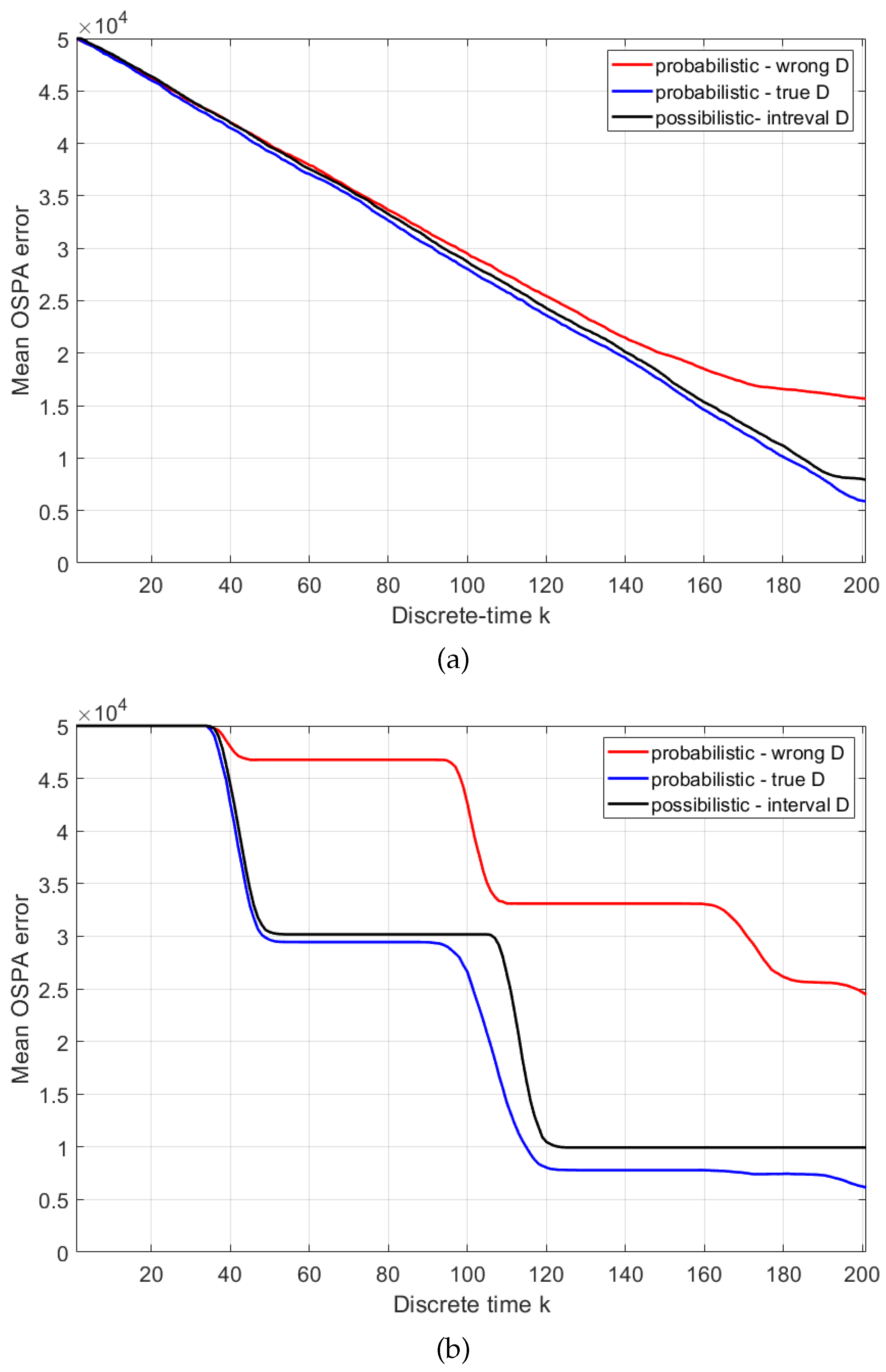
The resulting three mean OSPA errors are presented in Figure 5 for two different target placements: (i) uniformly random target locations across the search area; (ii) random placement in two squares positioned in diagonal corners of the search area. Mean OSPA line colours in Figure 5 are as follows: black for possibilistic search, blue for probabilistic - using true D (i.e., ideal case (a) above); red for probabilistic - using wrong D (i.e., case (b)). All three mean OSPA error curves follow the same trend: they reduce steadily from the initial value of c, as the searching agent traverses the area along the spiral path and discovers the targets. Of the three comparing methods, as expected, the best performance (i.e., the smallest OSPA error) is achieved using the probabilistic with true D (ideal case). The possibilistic solution, which operates using the available interval-valued probability of detection, is fairly close to the ideal case. Finally, the probabilistic, using the wrong value of D is the worst. The difference in performance is particularly dramatic when the placement of targets is non-uniform.
6. Conclusions
The paper formulated a solution to autonomous search for targets in the framework of possibility theory. The main rational for the possibilistic formulation is its ability to deal with epistemic uncertainty, expressed by partially known probabilistic models. In this paper, we focused on the interval-valued probability of detection (as a function of range). The paper presented Bayes-like update equations for the information state in the possibilistic framework, as well as an epistemic reward function for motion control. The numerical results demonstrated that the proposed possibilstic formulation of search can deal effectively with epistemic uncertainty in the form of interval-valued probability of detection. As expected, the (conventional) probabilistic solution performs (sightly) better when the correct precise model of the probability of detection is known (the ideal model-match case). However, the probabilistic solution can result in dramatically worse performance if an incorrect precise model is adopted.
Author Contributions
Conceptualization, Branko Ristic; Investigation, Zhijin Chen; Methodology, Zhijin Chen, Branko Ristic and Du Yong Kim; Software, Zhijin Chen; Supervision, Branko Ristic and Du Yong Kim; Validation, Zhijin Chen; Writing – original draft, Zhijin Chen; Writing – review & editing, Branko Ristic and Du Yong Kim.
Funding
Zhijin Chen is supported by an Australian Government Research Training Program (RTP) Scholarship.
Conflicts of Interest
The authors declare no conflict of interest.
References
- M. F. Shlesinger, “Search research,” Nature, vol. 443, no. 7109, pp. 281–282, 2006. [CrossRef]
- L. D. Stone, J. O. Royset, and A. R. Washburn, Optimal search for moving targets. Springer, 2016.
- A. Marjovi and L. Marques, “Multi-robot olfactory search in structured environment,” Robotics and Autonomous Systems, vol. 59, pp. 867–881, 2011. [CrossRef]
- R. R. Pitre, X. R. Li, and R. Delbalzo, “UAV route planning for joint search and track missions—an information-value approach,” IEEE Transactions on Aerospace and Electronic Systems, vol. 48, no. 3, pp. 2551–2565, 2012. [CrossRef]
- J. Burgués and S. Marco, “Environmental chemical sensing using small drones: A review,” Science of The Total Environment, p. 141172, 2020. [CrossRef]
- M. Park, S. An, J. Seo, and H. Oh, “Autonomous source search for UAVs using Gaussian mixture model-based infotaxis: Algorithm and flight experiments,” IEEE Transactions on Aerospace and Electronic Systems, vol. 57, no. 6, pp. 4238–4254, 2021. [CrossRef]
- B. O. Koopman, “Search and screening,” OEG Rep., 1946.
- P. A. Bakut and Y. V. Zhulina, “Optimal control of cell scanning sequence in search for objects,” Engineering Cybernetics, vol. 9, pp. 740–746, 1971.
- D. W. Krout, W. L. J. Fox, and M. A. El-Sharkawi, “Probability of target presence for multistatic sonar ping sequencing,” IEEE Journal of Oceanic Engineering, vol. 34, no. 4, pp. 603–609, 2009. [CrossRef]
- D. Angley, B. Ristic, W. Moran, and B. Himed, “Search for targets in a risky environment using multi-objective optimisation,” IET Radar, Sonar & Navigation, vol. 13, no. 1, pp. 123–127, 2019. [CrossRef]
- R. J. Kendall, S. M. Presley, G. P. Austin, and P. N. Smith, Advances in biological and chemical terrorism countermeasures. CRC Press, 2008.
- T. Furukawa, L. C. Mak, H. Durrant-Whyte, and R. Madhavan, “Autonomous Bayesian search and tracking, and its experimental validation,” Advanced Robotics, vol. 26, no. 5-6, pp. 461–485, 2012. [CrossRef]
- B. Ristic, A. Skvortsov, and A. Gunatilaka, “A study of cognitive strategies for an autonomous search,” Information Fusion, vol. 28, pp. 1–9, 2016. [CrossRef]
- K. Haley, Search theory and applications. Springer Science & Business Media, 2012, vol. 8.
- E. K. P. Chong, C. M. Kreucher, and A. O. Hero, “POMDP approximation using simulation and heuristics,” in Foundations and Applications of Sensor Management. Springer, 2008, pp. 95–119.
- A. O. Hero III, C. M. Kreucher, and D. Blatt, “Information theoretic approaches to sensor management,” Foundations and applications of sensor management, pp. 33–57, 2008. [CrossRef]
- F. Hampel, “Nonadditive probabilities in statistics,” Journal of Statistical Theory and Practice, vol. 3, no. 1, pp. 11–23, 2009. [CrossRef]
- L. A. Zadeh, “Fuzzy sets as a basis for a theory of possibility,” Fuzzy sets and systems, vol. 1, no. 1, pp. 3–28, 1978. [CrossRef]
- R. R. Yager and L. Liu, Classic works of the Dempster-Shafer theory of belief functions. Springer, 2008, vol. 219.
- P. Walley, Statistical reasoning with imprecise probabilities. Springer, 1991, vol. 42. [CrossRef]
- D. Dubois, H. Prade, and S. Sandri, “On possibility/probability transformations,” Fuzzy logic: State of the art, pp. 103–112, 1993. [CrossRef]
- D. Dubois and H. Prade, “Possibility theory and its applications: Where do we stand?” Springer Handbook of Computational Intelligence, pp. 31–60, 2015. [CrossRef]
- B. Ristic, J. Houssineau, and S. Arulampalam, “Robust target motion analysis using the possibility particle filter,” IET Radar, Sonar & Navigation, vol. 13, no. 1, pp. 18–22, 2019. [CrossRef]
- ——, “Target tracking in the framework of possibility theory: The possibilistic Bernoulli filter,” Information Fusion, vol. 62, pp. 81–88, 2020. [CrossRef]
- Z. Chen, B. Ristic, J. Houssineau, and D. Y. Kim, “Observer control for bearings-only tracking using possibility functions,” Automatica, vol. 133, p. 109888, 2021. [CrossRef]
- J. Houssineau, J. Zeng, and A. Jasra, “Uncertainty modelling and computational aspects of data association,” Statistics and Computing, vol. 31, no. 5, pp. 1–19, 2021. [CrossRef]
- B. Ristic, “Target tracking in the framework of possibility theory,” ISIF Perspectives of information fusion, vol. 6, pp. 47–48, June 2023. [CrossRef]
- J. Houssineau and A. N. Bishop, “Smoothing and filtering with a class of outer measures,” SIAM/ASA Journal on Uncertainty Quantification, vol. 6, no. 2, pp. 845–866, 2018. [CrossRef]
- A. N. Bishop, J. Houssineau, D. Angley, and B. Ristic, “Spatio-temporal tracking from natural language statements using outer probability theory,” Information Sciences, vol. 463, pp. 56–74, 2018. [CrossRef]
- J. Houssineau, “A linear algorithm for multi-target tracking in the context of possibility theory,” IEEE Transactions on Signal Processing, vol. 69, pp. 2740–2751, 2021. [CrossRef]
- M. Boughanem, A. Brini, and D. Dubois, “Possibilistic networks for information retrieval,” International Journal of Approximate Reasoning, vol. 50, no. 7, pp. 957–968, 2009. [CrossRef]
- B. Ristic, C. Gilliam, M. Byrne, and A. Benavoli, “A tutorial on uncertainty modeling for machine reasoning,” Information Fusion, vol. 55, pp. 30–44, 2020. [CrossRef]
- L. M. De Campos, J. F. Huete, and S. Moral, “Probability intervals: A tool for uncertain reasoning,” Intern. Journal of Uncertainty, Fuzziness and Knowledge-Based Systems, vol. 2, no. 02, pp. 167–196, 1994. [CrossRef]
- M.-H. Masson and T. Denoeux, “Inferring a possibility distribution from empirical data,” Fuzzy sets and systems, vol. 157, no. 3, pp. 319–340, 2006. [CrossRef]
- G. J. Klir and R. M. Smith, “On measuring uncertainty and uncertainty-based information: Recent developments,” Annals of Mathematics and Artificial Intelligence, vol. 32, pp. 5–33, 2001. [CrossRef]
- J. Abellán, “Uncertainty measures on probability intervals from the imprecise dirichlet model,” Intern. Journal of General Systems, vol. 35, no. 5, pp. 509–528, 2006. [CrossRef]
- M. Pota, M. Esposito, and G. De Pietro, “Transforming probability distributions into membership functions of fuzzy classes: A hypothesis test approach,” Fuzzy Sets and Systems, vol. 233, pp. 52–73, 2013. [CrossRef]
- Y. Bar-Shalom, X. R. Li, and T. Kirubarajan, Estimation with applications to tracking and navigation: Theory algorithms and software. John Wiley & Sons, 2004.
- D. Schuhmacher, B.-T. Vo, and B.-N. Vo, “A consistent metric for performance evaluation of multi-object filters,” IEEE Transactions on Signal Processing, vol. 56, no. 8, pp. 3447–3457, 2008. [CrossRef]
| 1 | Specification of a possibility function from a probability mass function expressed by probability intervals is not unique. For example, another more involved method for this task is via the maximum specificity criterion [34]. |
| 2 | |
| 3 |
Figure 1.
Simulation setup: the cyan stars indicate the true targets; the blue dotted line is the trajectory of the searching agent up to steps; the red dots indicate detections at .
Figure 1.
Simulation setup: the cyan stars indicate the true targets; the blue dotted line is the trajectory of the searching agent up to steps; the red dots indicate detections at .

Figure 2.
The imprecise model of the probability of detection D used in simulations. The true D is plotted with the blue solid line.
Figure 2.
The imprecise model of the probability of detection D used in simulations. The true D is plotted with the blue solid line.
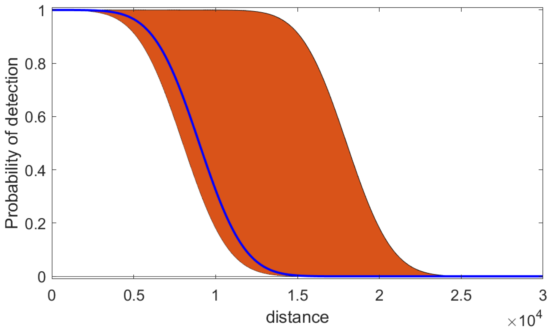
Figure 3.
Posterior possibility maps at time : (a) Target presence map ; (b) Target absence map (white colour implies zero possibility)
Figure 3.
Posterior possibility maps at time : (a) Target presence map ; (b) Target absence map (white colour implies zero possibility)
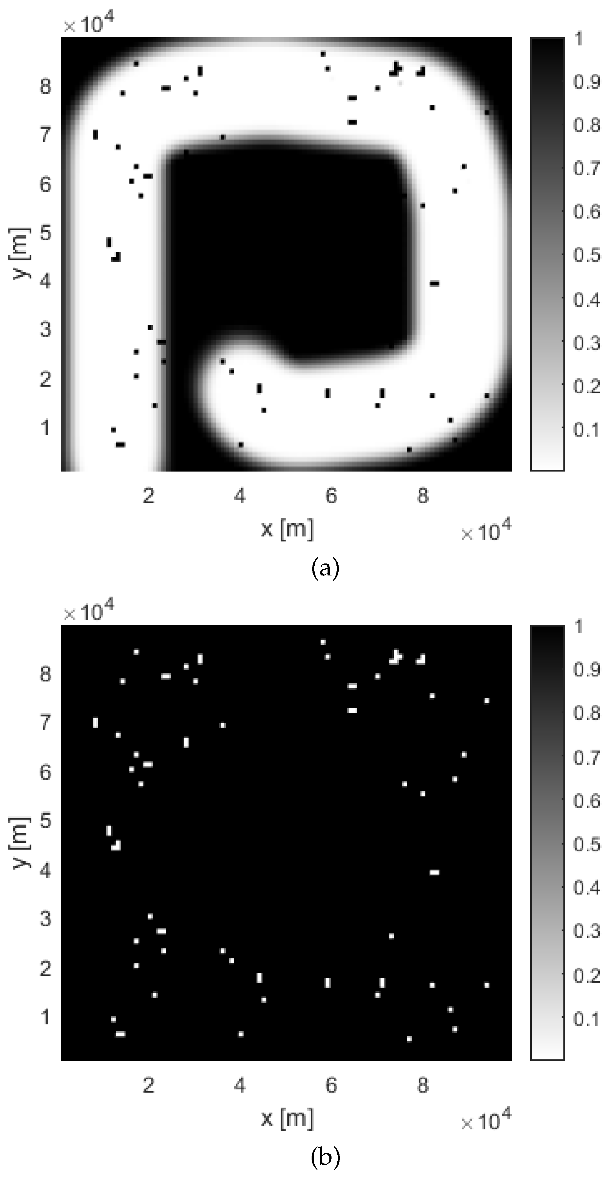
Figure 4.
Output of the search algorithm: Estimated target locations (indicated by red asterisks)
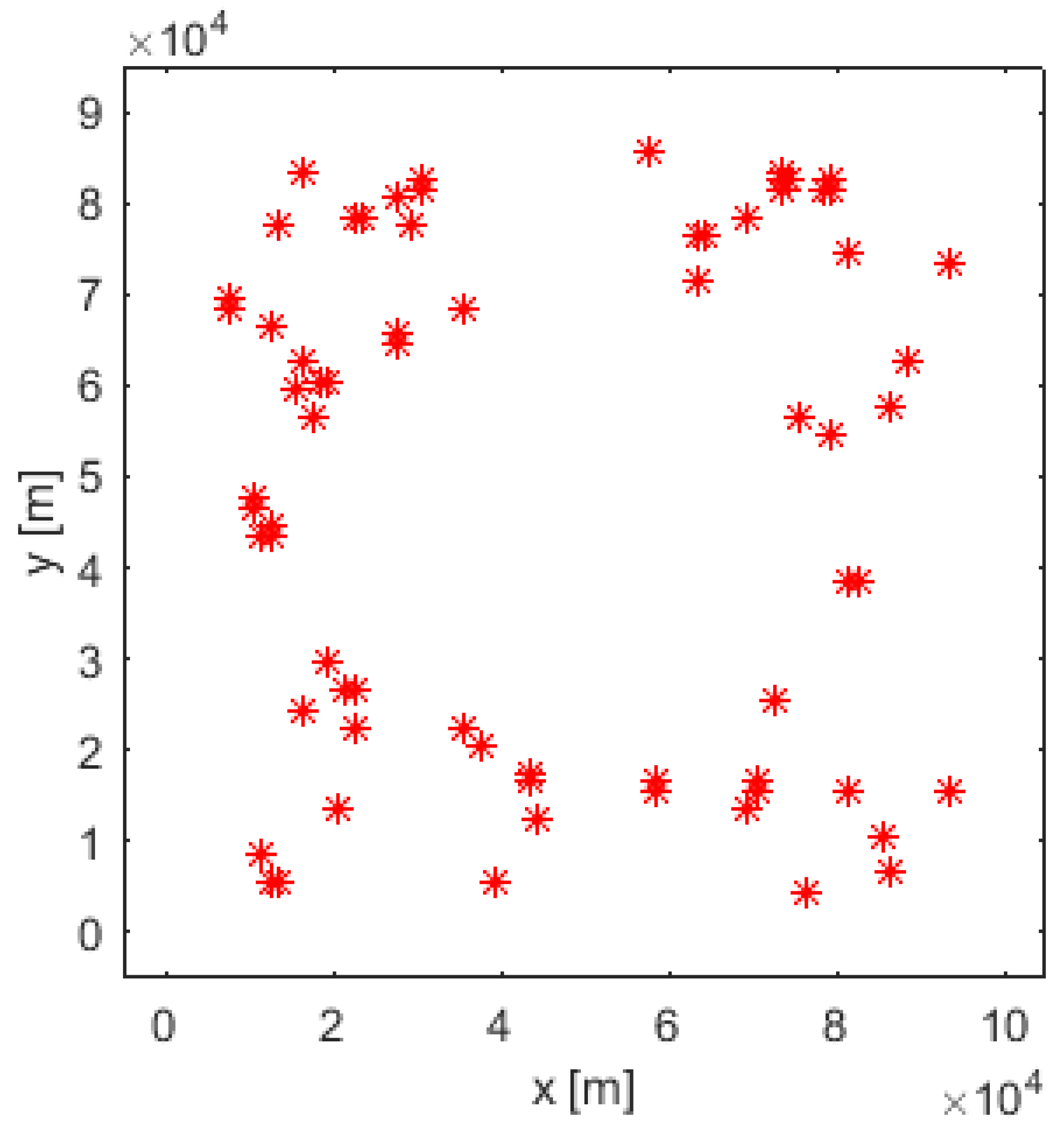
Figure 5.
Mean OSPA errors obtained from 100 Monte Carlo runs. The scenario involves 80 targets placed at (a) uniformly random locations; (b) uniformly random locations of two diagonal squares in the search area.
Figure 5.
Mean OSPA errors obtained from 100 Monte Carlo runs. The scenario involves 80 targets placed at (a) uniformly random locations; (b) uniformly random locations of two diagonal squares in the search area.
Disclaimer/Publisher’s Note: The statements, opinions and data contained in all publications are solely those of the individual author(s) and contributor(s) and not of MDPI and/or the editor(s). MDPI and/or the editor(s) disclaim responsibility for any injury to people or property resulting from any ideas, methods, instructions or products referred to in the content. |
© 2024 by the authors. Licensee MDPI, Basel, Switzerland. This article is an open access article distributed under the terms and conditions of the Creative Commons Attribution (CC BY) license (http://creativecommons.org/licenses/by/4.0/).
Copyright: This open access article is published under a Creative Commons CC BY 4.0 license, which permit the free download, distribution, and reuse, provided that the author and preprint are cited in any reuse.