
Submitted:
22 May 2024
Posted:
23 May 2024
You are already at the latest version
Abstract
Fluidized beds are pivotal in the process industry and chemical engineering, with Computational Fluid Dynamics (CFD) playing a crucial role in their design and optimization. Challenges in CFD modeling stem from the scarcity or inconsistency of experimental data for validation, along with the uncertainties introduced by numerous parameters and assumptions across different CFD codes. This study navigates these complexities by comparing simulation results from the open-source MFIX and OpenFOAM, and the commercial ANSYS FLUENT, against experimental data. Utilizing a Eulerian-Eulerian framework and the kinetic theory of granular flow (KTGF), the investigation focuses on solid-phase properties through the classical drag laws of Gidaspow and Syamlal-O’Brien across varied parameters. Findings indicate that ANSYS Fluent, MFiX, and OpenFOAM can achieve reasonable agreement with experimental benchmarks, each showcasing distinct strengths and weaknesses. The study also emphasizes that both the Syamlal-O’Brien and Gidaspow drag models exhibit reasonable agreement with experimental benchmarks across the examined CFD codes, suggesting a moderated sensitivity to the choice of drag model. Moreover, the analysis were also carried out for 2D and 3D simulations, revealing that the dimensional approach impacts the predictive accuracy to a certain extent, with both models adapting well to the complexities of each simulation environment. The study highlights the significant influence of restitution coefficients on bed expansion due to their effect on particle-particle collisions, with a value of 0.9 deemed optimal for balancing simulation accuracy and computational efficiency. Conversely, the specularity coefficient, impacting particle-wall interactions, exhibits a more subtle effect on bed dynamics. This finding emphasizes the critical role of carefully choosing these coefficients to effectively simulate the nuanced behaviors of fluidized beds.
Keywords:
Fluidized beds
; CFD
; Multiphase Flow
; Fluidization
; Fluent
; OpenFOAM
; MFiX
1. Introduction
Fluidized beds are one of the most widely used chemical reactors in many industry areas. It has been used mostly for gas-solid reactions as it provides some advantages including its easiness of handling and transport of solids due to fluid-like behavior, intensive mixing of solids leads to a consistent temperature distribution and favorable conditions for heat and mass transfer. [1]. Despite its advantages, it has also some drawbacks which heavily relies upon then complexity of hydrodynamics behavior and the difficulty in scaling up the reactor [1,2]. Historically, empirical methodologies derived from laboratory-scale investigations of fluidized-bed reactors have been instrumental in calculating key operational parameters, such as minimum fluidization velocity, bubble dynamics, particle attrition rates, and the axial distribution of solid mass fractions [3].
Numerical simulations offer a shortcut to circumvent the extensive process involved in designing and executing experiments, enabling rapid assessment of relevant fields at the industrial scale [4]. One of the numerical methods widely used is so-called Computational fluid dynamics (CFD). Several CFD models exist for simulating gas-solid flows, including the two-fluid model, discrete-particle model, hybrid model, and direct numerical simulations. The two-fluid method, particularly its most utilized form, the Eulerian-Eulerian (E-E) approach, considers both phases as interpenetrating continua. Closure relations based on the kinetic theory of granular flows (KTGF) help describe the solid phase with gas-like properties, considering the particles’ motion influenced by interactions within the gas phase and with other particles or walls [5]. In the discrete-particle approach, the fluid phase is treated as a continuum, while the solid phase is considered discrete, tracking individual particles within the computational domain. This method, notably utilized in the Eulerian-Lagrangian (E-L) framework, is recognized for its unique particle collision detection, which can be either stochastic or deterministic, facilitating detailed analysis of particle dynamics [6]. In the hybrid methods, the two-fluid and discrete-particle are integrated to leverage both models’ benefits. This sub-domain method simplifies the computational domain based on an equilibrium index, optimizing simulation efficiency and accuracy [7]. In Direct Numerical Simulation (DNS), it solves directly the Navier-Stokes equation aiming to capture the full range of scales and dynamics by using high-resolution grids and accurate numerical schemes. However, DNS is also limited by its high computational cost and low Reynolds numbers [8].
Over the past 20 years, numerous studies on gas-solid CFD models have been conducted using commercial CFD software, e.g., ANSYS FLUENT [9], ANSYS CFX [10], OpenFOAM [11], MFiX [12], BARRACUDA Virtual Reactor [13], CFDEM coupling [14], COMSOL Multiphysics [15], STAR-CCM [16] and EDEM [17]. Given the fluidized bed’s complex hydrodynamics, researchers focus on examining various parameters that influence gas-solid flow dynamics. Essential factors to consider in numerical models include superficial gas velocity, drag, specularity and restitution coefficients, and frictional viscosity, as these significantly affect the behavior of fluidized beds [18].
Taghipour et al. [19] compared hydrodynamics in a fluidized bed through experiments and FLUENT 6.0 simulations. The study used a pseudo-2D experimental setup and a 2D Eulerian-Eulerian model incorporating Gidaspow [5], Syamlal-O`Brien [20], and Wen-Yu drag models. Results showed the bed reaching steady state in 3 seconds, with consistent bed expansion and bubble formation. While the drag models closely matched experimental observations, discrepancies in voidage and bed expansion highlighted the need for further CFD model validation.
Cornelissen et al. [21] investigated the impact of mesh size, time step, and convergence criteria on the accuracy of a liquid-solid fluidized bed model in FLUENT 6.1.22, benchmarking their findings against experimental data. They determined that a convergence criterion of led to faster, convergent results compared to the standard . Additionally, they noted that Courant numbers within the range of to produced reliable outcomes regardless of mesh size and time step.
Li et al. [22] explored how solid phase boundary conditions affect simulations by adjusting specularity and particle-wall restitution coefficients in both 2D and 3D Eulerian-Eulerian models using MFIX software, comparing results to a pseudo 2D experiment. They discovered that the restitution coefficient’s impact was minimal compared to the specularity coefficient, with specularity coefficients under 0.05 leading to notable deviations in solid flow near walls and altering circulation patterns. While both 2D and 3D simulations captured the general flow behavior, 3D simulations aligned more closely with experimental data, emphasizing the significance of wall effects in pseudo 2D experiments for CFD model validation.
Herzog et al. [23] conducted a comparative analysis using MFIX, OpenFOAM versions 1.6/2.0, and FLUENT 6.3 against experimental findings by Taghipour, focusing on a 2D Eulerian-Eulerian using Gidaspow and Syamlal O`Brien drag models. The study revealed that FLUENT and MFIX closely matched experimental data for both drag models, whereas OpenFOAM’s predictions were not satisfactory, suggesting OpenFOAM requires further refinement and validation for fluidization prediction.
Shi et al. [18] carried out the research to align 2D and 3D models with Taghipour et al. [19] experimental findings, utilizing Eulerian-Eulerian frameworks in FLUENT 16.2. Their investigation spanned dimensions, flow regimes, boundary conditions, mesh granularity, and drag models. Optimal grid size emerged as 18 times the particle diameter for closest experimental alignment, with finer meshes diminishing accuracy. Minor variances were observed within specific specularity and restitution coefficient ranges, deeming them suitable. Turbulence’s impact was minimal within the bed but influenced gas flow above, recommending laminar models for non-reactive, isothermal beds and RANS models otherwise. Syamlal-O`Brien drag models, particularly with Johnson-Jackson boundary conditions and turbulent RANS models, showed superior experimental congruence. They noted 3D models matched experimental data more closely than 2D, cautioning that certain 2D model parameter combinations might mislead due to unrealistic assumptions. Consequently, they advocated for 3D validations, reserving 2D analyses for pre-validated model sensitivity studies.
In the current study, the fluidized bed columns from Taghipour et al. [19] were analyzed in both 2D and 3D simulations using three different CFD software codes: ANSYS Fluent 2023 R3, MFiX 23.1.1, and OpenFOAM 10. Simulations in MFiX and OpenFOAM were realized as part of the MSc thesis of Daun [24]. The current work extends the analysis presented by [24], and compares results further with new simulations realized in ANSYS Fluent. This investigation included the examination of two drag models, Syamlal-O’Brien and Gidaspow, across varied superficial gas velocities. Additionally, the study explored the effects of varying restitution and specularity coefficients. Simulations employed a Eulerian-Eulerian framework underpinned by the kinetic theory of granular flow (KTGF) aiming to highlight and address the subtleties inherent in inter-software comparisons.
2. Problem Description
The observation of several parameters as outlined previously was done by replicating the experimental case from Taghipour et al. [19] as it enables modelling validation by comparing to the experimental results therein. The model’s geometry consists of a rectangular column, measuring 0.28 m in width, 1 m in height, and 0.025 m in depth. The lower section of the column, extending up to 0.4 meters, is densely packed with granular particles with mean particle size of 275 m at a packing density of 0.6, illustrated in Figure 1. According to Taghipour et al. [19] the minimum fluidization velocity () is 0.065 m/s, whereas the system exhibited an overall pressure drop of 4400 Pa, a bed expansion ratio of 1.1, and a voidage (gas-phase volume fraction) of 0.5.
3. Computational Model
In this work, the simulations were carried out in the framework of Eulerian-Eulerian (E-E) by utilizing the kinetic theory of granular flow (KTGF). Three different CFD codes, namely, ANSYS Fluent version 2023 R3, MFiX 23.1.1 and OpenFOAM 10 were evaluated along with the implementation of Syamlal-O`Brien and Gidaspow drag model by varying superficial gas velocities up to 0.03, 0.1, 0.38, 0.46, and 0.51 m/s, equivalent to 0.5, 1.5, 6, 7, and 8 times the minimum fluidization velocity (). The complete selected simulation model parameters are summarized in Table 1. The governing equation and simulation setting of ANSYS Fluent, MFiX and OpenFOAM for developing the fluidized bed simulation model are explained below.
3.1. Governing Equation
The governing equations used in this simulation of fluidized bed for air and glass beads case can be summarized as follows:
Mass balance equations
Where , , , , and represent the volume fraction, velocity and density of gas phase and solid phase respectively. The total volume fraction of gas and solid phase is equal to unity:
Momentum balance equations
Where represents the momentum exchange coefficient or interphase drag force coefficient which will be given by following Syamlal-O`Brien and Gidaspow drag models. The terms and represent the deviatoric stress tensors for the gas and solid phases, respectively. Pressure gradients are accounted for by in the gas phase and in the solid phase. The gravitational force is represented by . The velocity of gas phase and solid phase are given by and .
Syamlal-O`Brien drag model [20]
where
and
where
with
A=, B= for , or
A=, B= for
Gidaspow drag model [5]
For
for
where
Solid phase fluctuating energy equations [28]
In order to attain closure of the solid stress terms in equation 4, 5 and 13 KTGF was used to derive the constitutive equations provided in in Table A1. KTGF provides values for solid-phase shear and bulk viscosities, as well as solid pressure. This theory evolves from Ogawa et al. [29]. It assumes particles are smooth, with inelastic and instantaneous binary collisions, as detailed by Gidaspow [5]. Drag models from Syamlal and O’Brien [20] and Gidaspow [5] were used in this study to calculate the momentum exchange coefficients as shown in equation 6 to 12. Conversely, the Gidaspow drag model merges the Wen-Yu drag model with the Ergun equation that is pertinent for dense beds, linking drag to pressure drop across porous media.
3.2. Simulation Setup
The OpenFOAM simulations adopted the fluidized bed tutorial case on multiphaseEulerFoam for fluidized Bed, whereas MFiX simulations used the 2D TFM fluid bed preset, and ANSYS Fluent based its setup on a 2D fluidized bed case from the training materials [30]. The computational domains for 2D and 3D models were discretized into 12,200 and 56,000 rectangular cells, respectively, with a grid width of m. Boundary conditions for all codes were set to default. Inlet velocities were varied, 0.03, 0.1, 0.38, 0.46, and 0.51 m/s. For the gas phase at the wall, a no-slip condition for the gas phase was applied at the walls. All three CFD codes facilitate the application of the Johnson and Jackson partial slip boundary condition for particles, enabling nuanced simulation of particle-wall interactions [31]. This formulation, articulated by Johnson and Jackson [31], prescribes boundary conditions for velocity and granular temperature in the solid phase, satisfying the specified requirements as outlined in equation 14 and 15. The default specularity coefficient of 0.2 and restitution coefficient of 0.9 for all codes.
Where K and represent the specularity and restitution coefficients respectively, their values are constrained between 0 and 1. A specularity coefficient (K) of 0 denotes perfectly specular collisions, whereas a value of 1 indicates perfectly diffuse collisions. Similarly, a restitution coefficient () of 0 corresponds to perfectly inelastic collisions, and a value of 1 represents perfectly elastic collisions. Motivated by the clear graphical analysis provided by [18], which elucidates the influence of these coefficients on fluidized bed flow behavior, this study set forth to investigate the effects of several restitution (0.9, 0.95, and 0.99) and specularity (0.05, 0.1, and 0.2) coefficient values to evaluate their impact on simulation results. In total, 50 simulation cases were executed, employing specific parameters i.e. CFD codes, superficial gas velocities, drag models, restitution coefficient, specularity coefficient and effect of 2D and 3D geometry as delineated in Table 3, to thoroughly investigate their effects.
Based on the sensitivity analysis conducted by Taghipour et al. [19] regarding time step and spatial discretization, minimal differences were observed between time steps of 0.0005s and 0.001s, and between second and first-order discretizations. Consequently, this study adopted a time step of 0.001s. In the discretization settings, ANSYS Fluent employed a first-order upwind and PRESTO for spatial discretization, alongside a first-order implicit method for temporal discretization. MFiX utilized a high order upwind scheme with a downwind factor for spatial discretization, incorporating the Superbee flux limiter. This approach was complemented by an implicit Euler method for temporal aspects. OpenFOAM’s strategy involved Gaussian discretization, applying flux limiters like "vanLeer" or "limitedLinear" based on the variable, highlighting a targeted approach to discretization.
The numerical settings included the use of the AMG solver coupled with the SIMPLE algorithm in ANSYS Fluent to address the software`s fluid flow challenges. MFiX and OpenFOAM utilized the PBiCGStab solver. MFiX employed a specific algorithm designed for its simulations [32], whereas OpenFOAM used the PIMPLE algorithm, indicating distinct computational strategies adopted by each software to navigate the complexities of multiphase flow simulations. Regarding convergence criteria, ANSYS Fluent was set to default settings for all variables at a tolerance of 0.001. OpenFOAM adopted strict tolerances, with 1e-9 for volume fraction (alpha.*), 1e-8 for pressure head (p_rgh) and velocity (U.*), and for temperature-related fields (Theta.*), with turbulence kinetic energy and its dissipation rate (k|epsilon.*) at 1e-5. MFiX set its default continuity tolerance at 0.001, with tolerances for energy, species, granular energy, and scalar variables at 0.0001. Under-relaxation factors were kept at default settings for ANSYS Fluent, OpenFOAM, and MFiX, reflecting a standard approach to ensuring numerical stability within each software framework.
4. Results
The results, derived from various simulations, are delineated in terms of bed expansion ratio (), pressure drop, solid volume fraction contour plots, solid velocity at m, and voidage at m. These results were obtained using three distinct CFD codes and evaluated across two drag models. The bed expansion ratio and pressure drop data encompass all examined superficial velocities: 0.03, 0.1, 0.38, 0.46, and 0.51 m/s, corresponding to 0.5, 1.5, 6, 7, and 8 times , respectively. In contrast, the solid volume fraction contour plots specifically showcase three selected superficial velocities: 0.2, 0.38, and 0.46 m/s, at times of 0.4 s, 1 s, and 3 s. Additionally, the analyses of solid velocity and voidage at m encapsulate the effects of variations across all two drag models, and the three CFD codes at 0.38 m/s of superficial gas velocity. The simulation outcomes, including bed expansion ratio, pressure drop, and voidage, were evaluated against the experimental results from Taghipour et al. [19], thereby assessing the simulations’ accuracy by using the formula for standard deviation as elucidated in Shi et al. [18].
4.1. Bed Expansion Ratio and Pressure Drop
The expansion of the bed was assessed by charting the time-averaged solid fraction at the bed’s center vertically. A criterion was established where a solid fraction value below 1% indicated the extent of bed expansion. This procedure was applied across various superficial gas velocities to observe how bed expansion varied with changes in inlet velocity. The summary of the results of bed expansion and pressure drop are summarized in Table 1. Figure 2 presents the bed expansions determined using the Syamlal-O`Brien drag model within Fluent, MFiX and OpenFOAM. From this figure, it is evident that all CFD codes forecast minimal bed expansion at lower velocities, with a linear increase in expansion noted for velocities exceeding 0.38 m/s. In 3D scenarios, bed expansion appears reduced compared to analogous 2D situations. Moreover, the figure illustrates that Fluent tends to forecast greater bed expansion compared to MFiX and OpenFOAM. Figure 3 illustrates the bed expansions observed when employing the Gidaspow drag model in MFiX and OpenFOAM. From this figure, it is apparent that three software packages register bed expansion at all velocities above the minimum fluidization velocity. The expansion appears to increase linearly in relation to the superficial gas velocity. The 3D simulations show a notably lesser degree of bed expansion compared to their 2D counterparts. A comparison with Figure 2 reveals that the expansions resulting from the Gidaspow model from OpenFOAM and MFiX exceed those observed with the Syamlal-O`Brien model. Surprisingly, Fluent forecasts lower bed expansions than OpenFOAM and MFiX when utilizing the Gidaspow model. Additionally, a contraction in the bed at the lowest gas velocity is noted in Fluent and MFiX with both drag models, a phenomenon not observed in OpenFOAM simulations.
The pressure drop across the bed was assessed at the outlet of the fluidized bed reactor for each tested superficial gas velocity. Figure 4 and Figure 5 illustrate a pattern where the pressure drop initially spikes to a peak value before gradually diminishing as the superficial gas velocity increases. It is observed that with the Gidaspow model, the peak pressure drop occurs at lower superficial gas velocities compared to the Syamlal-O`Brien model. Additionally, both figures indicate that MFiX and Fluent estimates a greater pressure drop across all tested superficial gas velocities than OpenFOAM, in both 2D and 3D simulations. A comparison between 2D and 3D results shows that Fluent and OpenFOAM reports a smaller pressure drop in 3D compared to 2D, whereas MFiX exhibits an increase in pressure drop from 2D to 3D simulations. It is also worth mentioning, specifically for Fluent, that the pressure drop at superficial velocities lower than the fluidization velocity tends to predict a very high pressure drop. This observation aligns with the findings from Taghipour et al. [19], El Ajouri et al. [33], suggesting that the primary cause could be attributed to the solids not being fully fluidized at these lower velocities, thereby being predominantly influenced by interparticle frictional forces. Such forces are not adequately predicted by the multifluid model used for simulating gas–solid phases in Fluent, which may not incorporate these frictional interactions effectively.
4.2. Solid Velocity and Voidage
Figure 6 displays the time-averaged solid particle velocity in the y-direction at a height of 0.2 meters, with a superficial gas velocity of 0.38 m/s, utilizing both Syamlal-O`Brien drag model in Fluent, MFiX and OpenFOAM. The observed trend across all data lines reveals a downward velocity near the walls transitioning to a parabolic upward velocity near the bed’s center. Notably, Fluent predicts significantly higher velocities than MFiX, particularly near the walls and the reactor’s center. Furthermore, for 3D simulations, velocities were averaged across the z-direction cells to align with the 2D results, offering a comprehensive view of the domain. While MFiX’s 3D outcomes closely resemble its 2D counterparts, OpenFOAM and Fluent markedly diverge, maintaining a relatively constant velocity across the bed as opposed to the parabolic profile observed in 2D simulations. In contrast to the Syamlal-O`Brien drag model, Figure 7 illustrates the time-averaged solid particle velocity using the Gidaspow drag model, processed similarly to Figure 6. The outcomes indicate that Fluent and MFiX yield nearly identical predictions, with velocities marginally higher at the bed’s center but displaying a somewhat flattened profile across both 3D and 2D simulations. Conversely, OpenFOAM’s results diverge slightly, showing higher velocities near the walls and at the center of the bed in both 3D and 2D scenarios. Notably, the 3D results in OpenFOAM exhibit a slightly flatter velocity profile compared to their 2D counterparts, suggesting a distinct behavior in spatial velocity distribution when using the Gidaspow model.
Further results, as shown in Figure 8, compare the time-averaged voidage for 2D and 3D simulations at the same bed height and gas velocity, employing the Syamlal-O’Brien drag model. This figure indicates that Fluent displays the highest voidage in 3D simulations compared to others, presenting an asymmetrical appearance relative to the rest. In OpenFOAM, the 3D simulations show a maximum voidage nearly identical to their 2D counterparts. Conversely, MFiX’s 3D simulations exhibit a zone of low voidage extending from the wall, which sharply increases to a peak significantly greater than that observed in 2D simulations at the center of the bed. On the other hand, Figure 9 showcases the time-averaged voidage for 2D and 3D simulations at the same bed height and gas velocity, utilizing the Gidaspow drag model. From this figure, it is evident that MFiX’s 3D simulations replicate the behavior observed in the Syamlal-O’Brien case, with voidage sharply increasing at the center of the bed in 3D simulations. For the Fluent simulations, both 2D and 3D present almost identical patterns, though the 3D simulations exhibit slightly higher voidage at the left wall. In OpenFOAM, the 3D results are slightly higher than 2D, maintaining a nearly similar pattern.
4.3. Solid Volume Fraction
The evolution of the fluidized beds and time averaged solid volume fractions with three chosen superficial gas velocities equal to 0.2, 0.38, and 0.46 m/s as the results from three different CFD codes with Syamlal-O`Brien drag model as well as Gidaspow drag model are depicted in Figure 10 and Figure 11. Initially, the bed height rose with the formation of bubbles until it stabilized at a constant steady-state height. The solid flow patterns inside the bed are relatively symmetrical for all cases before t < 3 s. The chaotic and transient bubble formation process at 3 seconds indicates that the statistical steady-state condition was achieved. Therefore, it confirmed the previous findings that a simulation duration of 3 seconds is sufficient to attain statistical steady-state behavior across all drag function models [19,23].
At the beginning of simulation, Fluent and MFiX display comparable patterns, with OpenFOAM showing slight deviations. As the flow progresses, the patterns of flow and bubble formation for both Syamlal-O’Brien and Gidaspow models remain similar in Fluent and MFiX but differ in OpenFOAM, highlighting that the numerical results of MFiX and Fluent are quite aligned, as also confirmed by Herzog et al. [23]. A closer examination reveals good agreement in the time-averaged solid volume fraction among all codes. All cases show a lower voidage observed near the wall and at the base of the bed, whereas an increased voidage is noted in the bed’s central area. This pattern of solid volume fraction distribution indicates a higher formation of bubbles in the central region as opposed to the bottom. Specifically, in the Syamlal-O`Brien model, Fluent exhibits a higher voidage and greater bed expansion compared to MFiX and OpenFOAM. Conversely, in the Gidaspow model, OpenFOAM demonstrates larger bed expansion and more voidage. The case studies with three superficial velocities further reveal that MFiX tends to display a more distinct phase border than OpenFOAM and Fluent, where phase interfaces blend more smoothly. This distinction appears to lead to the formation of more, but smaller, bubbles in OpenFOAM, whereas MFiX features fewer but significantly larger bubbles, highlighting the intricate dynamics of fluidized beds as captured by different simulation tools and drag models.
5. Discussion
Fluidized beds continue to be indispensable in the industrial sector, a fact underscored by the extensive volume of research utilizing Computational Fluid Dynamics (CFD) codes for their study, as elaborately discussed by Alobaid et al. [4]. This significant focus on fluidized beds through CFD simulations brings to the forefront the necessity of determining the most suitable CFD software for accurately capturing the complex hydrodynamics within these systems. Among the available CFD tools, ANSYS Fluent and MFiX have been recognized for their maturity and reliability in modeling fluidized bed dynamics. In contrast, OpenFOAM, despite its potential, has faced skepticism regarding its accuracy and applicability for fluidized bed simulations, as highlighted by Herzog et al. (2012). In this context, our study undertook on a comparative evaluation of these three CFD codes by simulating a standard fluidized bed configuration and comparing the outcomes with the experimental findings reported by Taghipour et al. [19]. In addition to that, the examination of each software’s numerical predictions of voidage fraction by employing the standard deviation formula as a measure of accuracy was also presented.
5.1. Comparative study of different codes
Figure 2 and Figure 3 showed a comparison between simulation results and experimental data for Syamlal-O`Brien and Gidaspow drag model, respectively. It is crucial to note that a challenge with the experimental data lies in the absence of a detailed description of how bed expansion measurements were conducted, limiting the direct comparability to the current simulation findings. Despite this, a general consistency in trends between simulated and experimental results is observable. For superficial velocities below 0.38 m/s using the Syamlal-O’Brien drag model, in the case of using Syamlal-O`Brien drag model, ANSYS Fluent tends to overestimate bed expansion, whereas MFiX and Fluent show a slight underestimation. However, starting from a superficial velocity of 0.38 m/s, all three software overestimate bed expansion. It’s noteworthy that results from 3D simulations presented lower bed expansion compared to their 2D counterparts, underscoring the significance of incorporating friction along the front and back walls, regardless of the drag model applied. While MFiX and OpenFOAM align closely with experimental outcomes, ANSYS Fluent consistently overestimates bed expansion, highlighting discrepancies across different CFD tools in predicting fluidized bed dynamics. This can also be clearly observed from the solid phase distribution pattern depicted in Figure 10, which shows that ANSYS Fluent, using the Syamlal-O’Brien drag model, exhibits higher bed expansion and significantly lower particle occupancy, or higher voidage, appearing much more fluidized compared to other software utilizing the same drag model. Conversely, with the Gidaspow drag model, the tendency of simulation results to overestimate bed expansion at and above 0.38 m/s persists. However, in this scenario, ANSYS Fluent typically underpredicts bed expansion, followed closely by MFiX, while OpenFOAM tends to slightly overpredict. Nonetheless, starting from a superficial velocity of 0.38 m/s, all three software solutions overestimate the bed expansion. Despite these tendencies, it is observed that findings from the 3D simulations align well with the experimental data.
The comparison of simulation outcomes with experimental data on pressure drop, employing the Syamlal-O’Brien and Gidaspow models, is illustrated in Figure 4 and Figure 5, respectively. Experimentally, the pressure drop is observed to sharply increase until reaching the minimum fluidization velocity, thereafter ascending more gradually with the rise in superficial gas velocity. Contrarily, numerical simulations diverge from this pattern, showing a sharp increase in pressure drop around the minimum fluidization velocity, followed by a gradual decrease as superficial gas velocity increases.
Notably, previous observations from OpenFOAM, as reported by Herzog et al. [23], indicated a significant overestimation of pressure drop. However, current results demonstrate that OpenFOAM now mirrors the trend seen in MFiX, with a pressure drop approximately 500 Pa lower. The introduction of a third dimension reveals differing impacts on pressure drop predictions between MFiX and OpenFOAM across both drag models. MFiX predicts a higher, and OpenFOAM a lower, pressure drop than their 2D simulations, deviating further from the experimental data. Conversely, with ANSYS Fluent, a distinct discrepancy is noted at a superficial velocity of 0.03 m/s across both drag models as previously explained in previous section. Across the board, ANSYS Fluent tends to overestimate pressure drops initially, then adjusts to underestimations. It is evident that no simulation perfectly aligns with the experimental data, with all predicted void fractions being overly large. Despite this, the outcomes could still be deemed in reasonable concordance with experimental observations. However, ANSYS Fluent gives a better fit to the experimental data at superficial velocities of 0.38 m/s and above. Furthermore, the introduction of the third dimension in ANSYS Fluent even results in a much better fit to the experimental result compare to MFiX and OpenFOAM. Notably, while the Syamlal-O`Brien and Gidaspow models yield broadly similar results, the Syamlal-O`Brien model slightly edges closer to the experimental data than Gidaspow in terms of pressure drop. It also align with the resport from Aboudaoud et al. [34] and Liu and Hinrichsen [35] which implied that Syamlal-O`Brien model is more suitable for pressure drop prediction compared to Gidaspow.
5.2. Simulation Error
To assess the accuracy of the numerical predictions of voidage fraction against experimental data from Taghipour et al. [19], the standard deviation profiles for both 2D and 3D simulations were calculated and are presented in Figure 12. The formula for standard deviation is given as follows:
where represents the estimated standard error, and are the experimental and predicted points of the voidage fraction along the x-coordinate at y = 0.2 m, respectively. The standard deviation serves as a reliable measure of error compared to other metrics since this method is derived from Linear Least Squares Regression commonly used in curve fitting. The standard deviation for 3D and 2D models falls within the range of 5.06 – 11.81 %. The findings suggest that neither 3D nor 2D simulations inherently guarantee closer agreement with experimental data. Interestingly, certain 2D simulations exhibit better alignment with the experimental data than their 3D counterparts, indicating that with appropriate parameter selection, 2D simulations can also be a viable option, as supported by Shi et al. [18].
By examining both the qualitative aspects presented in Figure 8 and Figure 9 and the quantitative data outlined in Figure 12, one can discern the impact of varying software and drag models on simulation outcomes. The results demonstrate that MFiX generally yields lower simulation discrepancies, followed by ANSYS Fluent and OpenFOAM. Notably, in the 3D context, MFiX and ANSYS Fluent exhibit similar levels of simulation error. Regarding the choice of drag model, the Syamlal-O`Brien model tends to produce lower simulation errors when used with MFiX and OpenFOAM, whereas the Gidaspow model appears to minimize simulation errors more effectively when applied in ANSYS Fluent. Consequently, while OpenFOAM holds potential for various applications, its performance in fluidized bed simulations appears to lag slightly behind that of MFiX and ANSYS Fluent, highlighting the importance of selecting the appropriate software and drag model to achieve the best simulation accuracy. This observation is consistent with the most significant differences in flow evolution between OpenFOAM and ANSYS Fluent and MFiX, as illustrated in Figure 10 and Figure 11. A previously discussed critical distinction lies in the phase interfaces within the simulations. OpenFOAM’s tendency to generate numerous and diffuse bubbles suggests that gas flow actively propels particles upwards across almost the entire domain. This phenomenon is visible in time-averaged plots from OpenFOAM, where a narrow region of particle accumulation along the wall is the only area where particles can descend. In contrast, MFiX and ANSYS Fluent simulations depict a different behavior, where smaller bubbles at the bed’s bottom coalesce into relatively larger and fewer distinct bubbles that ascend through the bed’s center.
5.3. The Effect of Restitution and Specularity Coefficient
The restitution coefficient is indicative of the collision behavior between particles in the fluidized bed, while the specularity coefficient represents the nature of collisions between particles and the walls. In this study, restitution coefficient values of 0.9, 0.95, and 0.99 were explored. According to the results presented in Table 1, a higher restitution coefficient leads to increased bed expansion in the Syamlal-O’Brien drag model, although it does not significantly affect the pressure drop. This trend is consistent with the Gidaspow drag model, where increasing the restitution coefficient also increases bed expansion, albeit with a slight decrease (0.013) between 0.9 and 0.95, followed by an increase at 0.99.
Analyzing the simulation results based on voidage measurement at y = 0.2 m at a superficial velocity of 0.38 m/s, it was observed that with both drag models, as the restitution coefficient increases (Syamlal-O’Brien: 10.03, 10.90, 13.57%; Gidaspow: 7.84, 8.40, 11.56%), the simulation error also increases this aligns with the result reported by Shi et al. [18]. This suggests that a restitution coefficient of 0.9 most accurately represents the conditions.
Conversely, regarding the impact of the specularity coefficient, which was varied between 0.05, 0.1, and 0.2, the results in the Syamlal-O’Brien drag model indicate that an increase in the specularity coefficient does not significantly alter bed expansion. However, in the Gidaspow drag model, a slight reduction in bed expansion was observed. The simulation error analysis within the Syamlal-O’Brien model correlates with bed expansion outcomes, showing minimal change across specularity coefficients (Syamlal-O’Brien: 10.51, 10.31, 10.03), suggesting that the influence of specularity coefficient variations on voidage predictions can be neglected, as also noted by Shi et al. [18]. Nonetheless, employing the Gidaspow model (Gidaspow: 7.45, 9.24, 7.84) reveals slight differences in simulation error values, with a notable increase at 0.1, indicating a sensitivity to specularity coefficient variations within the Gidaspow drag model.
6. Conclusions
In the current study, the gas-solid flow within 2D and 3D fluidized bed columns, replicated from Taghipour et al. [19], was simulated using the Eulerian-Eulerian framework coupled with the Kinetic Theory of Granular Flow (KTGF). This investigation aimed to assess the capabilities of three prominent CFD software packages—ANSYS Fluent, MFiX, and OpenFOAM—in modeling fluidized bed dynamics. The study specifically focused on the application of the Syamlal-O’Brien and Gidaspow drag models across varying superficial velocities, restitution coefficients, and specularity coefficients to provide a comprehensive evaluation of these tools. The key findings of this research are summarized as follows:
- The assessment of ANSYS Fluent, MFiX, and OpenFOAM showed they could achieve reasonable agreement with experimental data across both drag models, offering insights into fluidized bed hydrodynamics. This comparison underscored specific strengths and weaknesses, revealing MFiX and ANSYS Fluent as more consistent and accurate in simulating fluidized bed dynamics, thereby emerging as preferable choices. OpenFOAM has shown maturity in predicting fluidized bed phenomena, yet it necessitates further validation and exploration to fully grasp the impact of various numerical settings and boundary conditions on its outcomes. This approach underscores the importance of fine-tuning and accurately assessing OpenFOAM’s capabilities for enhanced reliability in fluidized bed simulations.
- The analysis of the Syamlal-O’Brien and Gidaspow drag models revealed significant differences in their predictions, particularly in terms of bed expansion and pressure drop. The Syamlal-O’Brien model, when used with MFiX and OpenFOAM, typically resulted in lower simulation errors compared to the Gidaspow model. However, ANSYS Fluent showed a preference for the Gidaspow model, indicating that the choice of drag model can significantly influence simulation outcomes and should be carefully considered based on the CFD software being used.
- The transition from 2D to 3D simulations introduced notable variations in bed expansion and pressure drop predictions. While 3D simulations offer a more detailed representation of fluidized bed dynamics, they do not always guarantee improved alignment with experimental data. In some cases, 2D simulations provided better fits, suggesting that the dimensionality of the simulation should be chosen based on specific study requirements and the expected flow behavior.
- The study showed that while higher restitution coefficients led to increased bed expansion, indicating their significant impact on particle-particle collisions, variations in the specularity coefficient, which affects particle-wall interactions, had a subtler influence on bed dynamics, particularly noted in the Gidaspow drag model. A restitution coefficient of 0.9 was identified as optimal, balancing accuracy and computational efficiency, whereas the specularity coefficient’s effect, though present, was less pronounced within the examined range. This emphasizes the necessity of carefully selecting these coefficients to accurately model the complex behaviors in fluidized beds.
Author Contributions
Conceptualization, K.E.E., P.F.D. and P.K. ; methodology, K.E.E., P.F.D. and P.K.; software, P.F.D. and P.K.; validation, P.F.D. and P.K.; formal analysis, P.F.D. and P.K.; investigation, P.F.D. and P.K.; resources, K.E.E.; data curation, P.F.D. and P.K.; writing—original draft preparation, P.K.; writing—review and editing, K.E.E., P.F.D. and P.K. ; visualization, P.F.D. and P.K.; supervision, K.E.E; project administration, K.E.E.; funding acquisition, K.E.E. All authors have read and agreed to the published version of the manuscript.
Funding
Financial support of the Norwegian Research Council, grant 337007, is acknowledged
Data Availability Statement
The data can be made available upon request from the corresponding author.
Conflicts of Interest
The authors declare no conflicts of interest.
Abbreviations
The following abbreviations are used in this manuscript:
| Volume fraction of the gas phase | |
| Volume fraction of the solid phase | |
| The maximum packing fraction of the solid phase | |
| Drag coefficient | |
| Diameter of the solid particles | |
| The rate of deformation tensor components for the solidphase | |
| A factor incorporating the restitution coefficient | |
| The restitution coefficient for solid-solid collisions | |
| Dissipation rate of fluctuating energy in the solidphase | |
| Collision dissipation of energy | |
| The radial distribution function at contact for solid-solidinteractions | |
| Gravitational acceleration vector | |
| The second invariant of the deformation tensor | |
| K | The specularity coefficient |
| Momentum exchange coefficient or interphase drag forcecoefficient | |
| Thermal conductivity of the solid phase for thefluctuating energy | |
| The thermal conductivity of the solid phase for granulartemperature | |
| Granular bulk viscosity | |
| Dynamic viscosity of the gas phase | |
| The viscosity coefficient of the solid phase | |
| Solid collision viscosity | |
| Solid frictional viscosity | |
| Solid kinetic viscosity | |
| ∇ | Nabla operator, representing vector differential operations |
| p | Pressure in the gas phase |
| Solid phase pressure | |
| Velocity vector of the gas phase | |
| Velocity vector of the solid phase | |
| Deviatoric stress tensor of the gas phase | |
| Solid phase shear stress tensor | |
| The identity tensor for the gas phase | |
| Gas phase shear stress tensor | |
| Deviatoric stress tensor of the solidphase | |
| Density of the gas phase | |
| Density of the solid phase | |
| ∅ | The angle of internal friction |
| t | Time |
| Fluctuating energy of the solid phase | |
| Relative velocity between phases | |
| Energy exchange rate between gas and solid phases | |
| Transfer of kinetic energy between gas and solid phases | |
| x | The spatial coordinate in the direction of the gradient |
| The transpose of the velocitygradient tensor of the gas phase | |
| Reynolds number for the solid phase, characterizing the flowregime |
Appendix A
Appendix A.1
The constitutive equations derived from KGTF is provided in below Table.

Table A1.
Constitutive equations used in this study
| Gas phase shear stress tensor |
| Solid phase shear stress tensor |
| Granular bulk viscosity |
| Solid shear viscosity |
| Solid collision viscosity [32] |
| Solid kinetic viscosity |
|
Syamlal-O`Brien [32]
|
| Solid frictional viscosity [27] |
|
|
| Solid phase pressure [26] |
| Radial distribution function [26,37] |
References
- Werther, J. Fluidized-Bed Reactors. In Ullmann’s Encyclopedia of Industrial Chemistry; John Wiley & Sons, Ltd, 2007; p. Article Number.
- Witt, P.M.; Hickman, D.A. Fluidized-bed reactor scale-up: Reaction kinetics required. AIChE Journal 2022, 68, e17803. [Google Scholar] [CrossRef]
- Kunii, D.; Levenspiel, O. Fluidization Engineering; Butterworth-Heinemann, 1991.
- Alobaid, F.; Almohammed, N.; Massoudi Farid, M.; May, J.; Rößger, P.; Richter, A.; Epple, B. Progress in CFD Simulations of Fluidized Beds for Chemical and Energy Process Engineering. Progress in Energy and Combustion Science 2022, 91, 100930. [Google Scholar] [CrossRef]
- Gidaspow, D. Multiphase flow and fluidization: continuum and kinetic theory descriptions; Academic Press: Boston, 1994. [Google Scholar]
- Stroh, A.; Alobaid, F.; Hasenzahl, M.T.; Hilz, J.; Ströhle, J.; Epple, B. Comparison of three different CFD methods for dense fluidized beds and validation by a cold flow experiment. Particuology 2016, 29, 34–47. [Google Scholar] [CrossRef]
- Grüner, C. Kopplung des Einzelpartikel-und des Zwei-Kontinua-Verfahrens für die Simulation von Gas-Feststoff-Strömungen; Shaker, 2004.
- Moin, P.; Mahesh, K. DIRECT NUMERICAL SIMULATION: A Tool in Turbulence Research. Annual Review of Fluid Mechanics 1998, 30, 539–578. [Google Scholar] [CrossRef]
- ANSYS Inc.. ANSYS FLUENT. Commercial software, 2023.
- ANSYS Inc.. ANSYS CFX. Commercial software, 2023.
- The OpenFOAM Foundation. OpenFOAM. General Public License, 2023.
- National Energy Technology Laboratory. MFiX. General Public License, 2023.
- CPFD Software. BARRACUDA Virtual Reactor. Commercial software, 2023.
- CFDEM project. LIGGGHTS CFDEM coupling. General Public License, 2023.
- COMSOL Inc.. COMSOL Multiphysics. Commercial software, 2023.
- CD-adapco. STAR-CCM+. Commercial software, 2023.
- Altair Engineering. EDEM. Commercial software, 2023.
- Shi, H.; Komrakova, A.; Nikrityuk, P. Fluidized beds modeling: Validation of 2D and 3D simulations against experiments. Powder Technology 2019, 343, 479–494. [Google Scholar] [CrossRef]
- Taghipour, F.; Ellis, N.; Wong, C. Experimental and computational study of gas–solid fluidized bed hydrodynamics. Chemical Engineering Science 2005, 60, 6857–6867. [Google Scholar] [CrossRef]
- Syamlal, M.; O’Brien, T.J. Simulation of granular layer inversion in liquid fluidized beds. International Journal of Multiphase Flow 1988, 14, 473–481. [Google Scholar] [CrossRef]
- Cornelissen, J.T.; Taghipour, F.; Escudié, R.; Ellis, N.; Grace, J.R. CFD modelling of a liquid–solid fluidized bed. Chemical Engineering Science 2007, 62, 6334–6348. [Google Scholar] [CrossRef]
- Li, T.; Grace, J.; Bi, X. Study of wall boundary condition in numerical simulations of bubbling fluidized beds. Powder Technology 2010, 203, 447–457. [Google Scholar] [CrossRef]
- Herzog, N.; Schreiber, M.; Egbers, C.; Krautz, H.J. A comparative study of different CFD-codes for numerical simulation of gas–solid fluidized bed hydrodynamics. Computers & Chemical Engineering 2012, 39, 41–46. [Google Scholar]
- Daun, P.F. A Comparative Study of Different CFD-codes for Fluidized Beds. Master’s thesis, NTNU, 2023.
- ANSYS, Inc.. Ansys Fluent Theory Guide. ANSYS, Inc., release 2021 r1 ed., 2021.
- Lun, C.K.K.; Savage, S.B.; Jeffrey, D.J.; Chepurniy, N. Kinetic theories for granular flow: inelastic particles in Couette flow and slightly inelastic particles in a general flowfield. Journal of Fluid Mechanics 1984, 140, 223–256. [Google Scholar] [CrossRef]
- Schaeffer, D.G. Instability in the evolution equations describing incompressible granular flow. Journal of Differential Equations 1987, 66, 19–50. [Google Scholar] [CrossRef]
- Ding, J.; Gidaspow, D. A bubbling fluidization model using kinetic theory of granular flow. AIChE Journal 1990, 36, 523–538. [Google Scholar] [CrossRef]
- Ogawa, S.; Umemura, A.; Oshima, N. On the equations of fully fluidized granular materials. Zeitschrift für angewandte Mathematik und Physik ZAMP 1980, 31, 483–493. [Google Scholar] [CrossRef]
- ANSYS, Inc.. Workshop: Modeling Uniform Fluidization in a 2D Fluidized Bed. ANSYS, Inc., release 2023 r1 ed., 2023.
- Johnson, P.C.; Jackson, R. Frictional–collisional constitutive relations for granular materials, with application to plane shearing. Journal of Fluid Mechanics 1987, 176, 67–93. [Google Scholar] [CrossRef]
- Syamlal, M.; Rogers, W.; O`Brien, T. MFIX documentation theory guide. Technical report, National Energy Technology Laboratory, U.S. Department of Energy, 1993.
- El Ajouri, O.; Lahlaouti, M.L.; Kharbouch, B. CFD-simulation of gas-solid flow in bubbling fluidized bed reactor. E3S Web of Conferences 2022, 336, 00059. [Google Scholar] [CrossRef]
- Aboudaoud, S.; Touzani, S.; Abderafi, S.; Cheddadi, A. CFD Simulation of Air-Glass Beads Fluidized Bed Hydrodynamics. Journal of Applied Fluid Mechanics 2023, 16. [Google Scholar]
- Liu, Y.; Hinrichsen, O. CFD modeling of bubbling fluidized beds using OpenFOAM®: Model validation and comparison of TVD differencing schemes. Computers & Chemical Engineering 2014, 69, 75–88. [Google Scholar]
- Gidaspow, D.; Bezburuah, R.; Ding, J. Hydrodynamics of Circulating Fluidized Beds: Kinetic Theory Approach, 1991.
- Carnahan, N.F.; Starling, K.E. Equation of State for Nonattracting Rigid Spheres. The Journal of Chemical Physics 1969, 51, 635–636. [Google Scholar] [CrossRef]
Figure 1.
The geometric setup used for simulations, adapted from Taghipour et al. [19].
Figure 1.
The geometric setup used for simulations, adapted from Taghipour et al. [19].
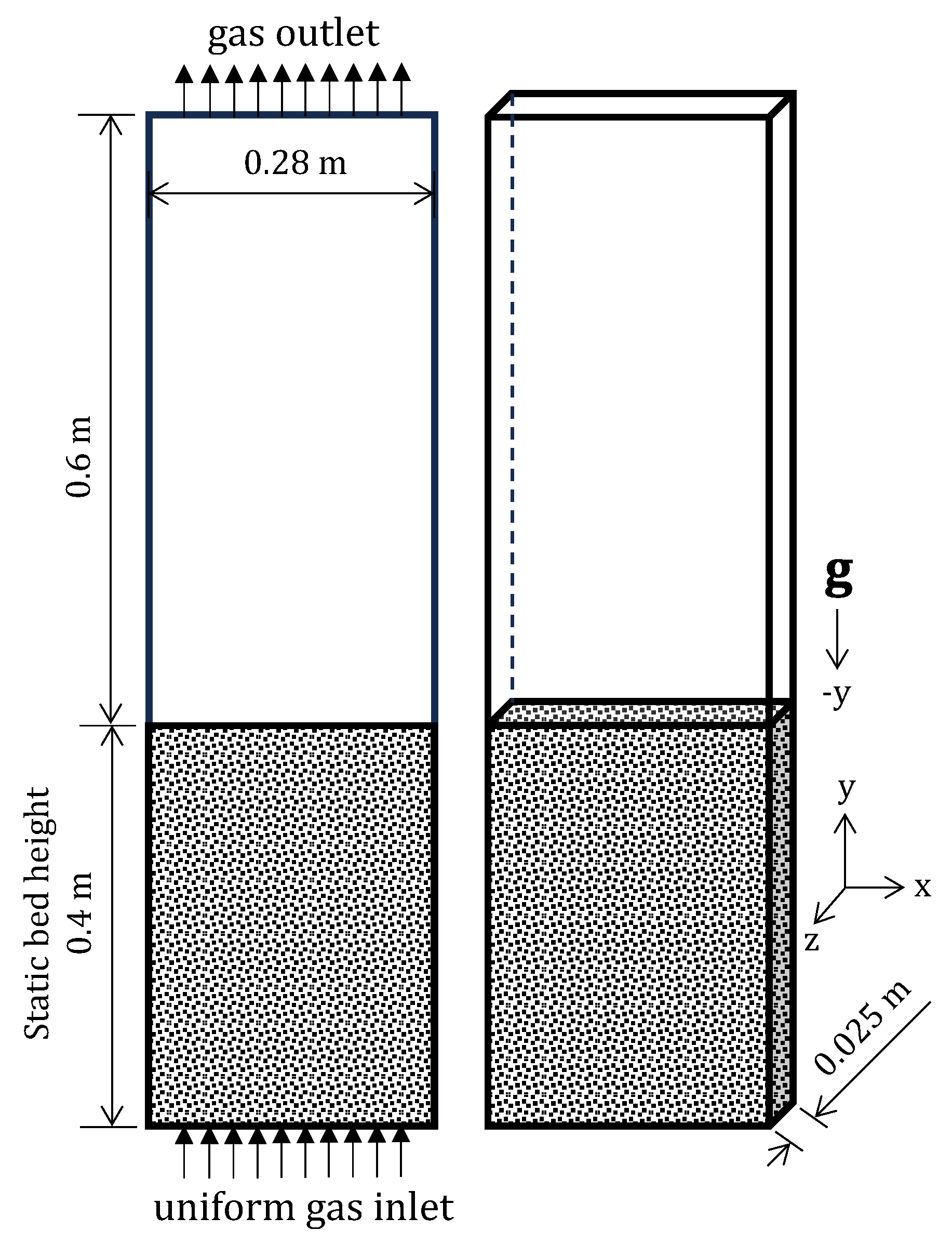
Figure 2.
Bed expansion for different superficial gas velocities with the Syamlal-O`Brien drag model in ANSYS Fluent, MFiX and OpenFOAM. Experiment data were taken from [19], with permission from Elsevier.
Figure 2.
Bed expansion for different superficial gas velocities with the Syamlal-O`Brien drag model in ANSYS Fluent, MFiX and OpenFOAM. Experiment data were taken from [19], with permission from Elsevier.
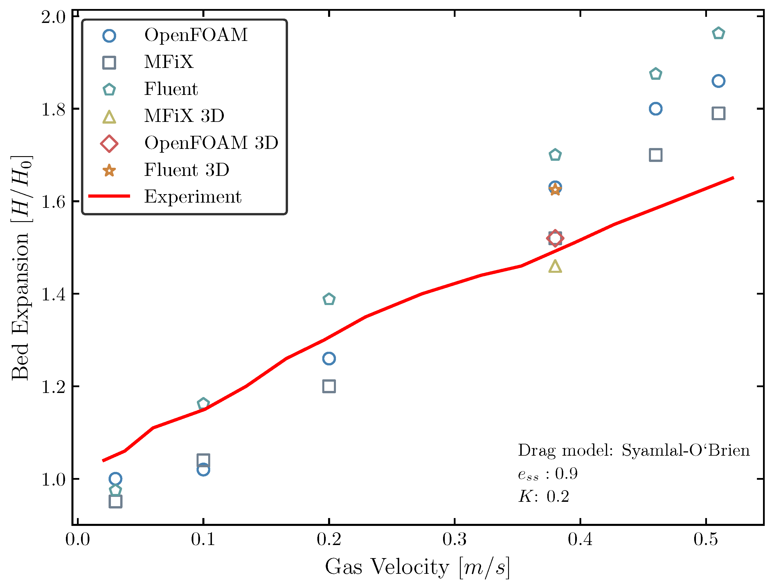
Figure 3.
Bed expansion for different superficial gas velocities with the Gidaspow drag model in ANSYS Fluent, MFiX and OpenFOAM. Experiment data were taken from [19], with permission from Elsevier.
Figure 3.
Bed expansion for different superficial gas velocities with the Gidaspow drag model in ANSYS Fluent, MFiX and OpenFOAM. Experiment data were taken from [19], with permission from Elsevier.
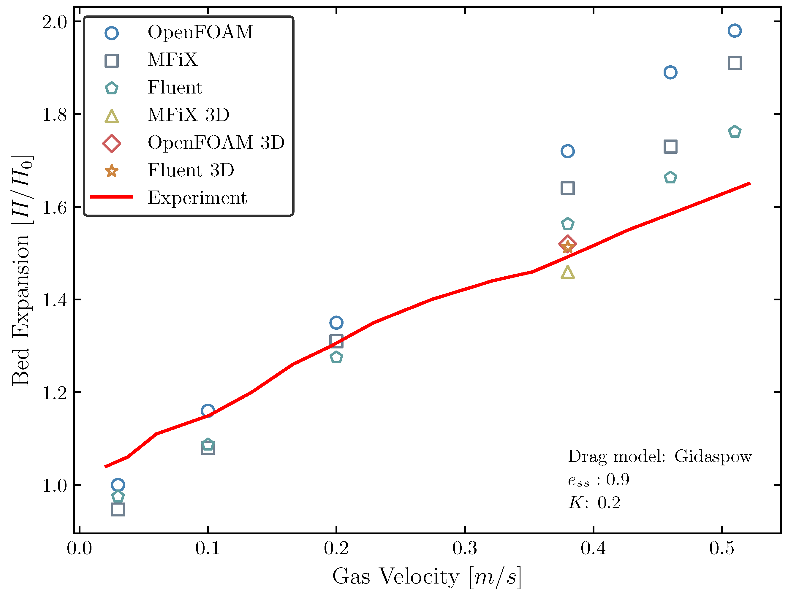
Figure 4.
Pressure drop for different superficial gas velocities with the Syamlal-O`Brien drag model in ANSYS Fluent, MFiX and OpenFOAM. Experiment data were taken from [19], with permission from Elsevier.
Figure 4.
Pressure drop for different superficial gas velocities with the Syamlal-O`Brien drag model in ANSYS Fluent, MFiX and OpenFOAM. Experiment data were taken from [19], with permission from Elsevier.
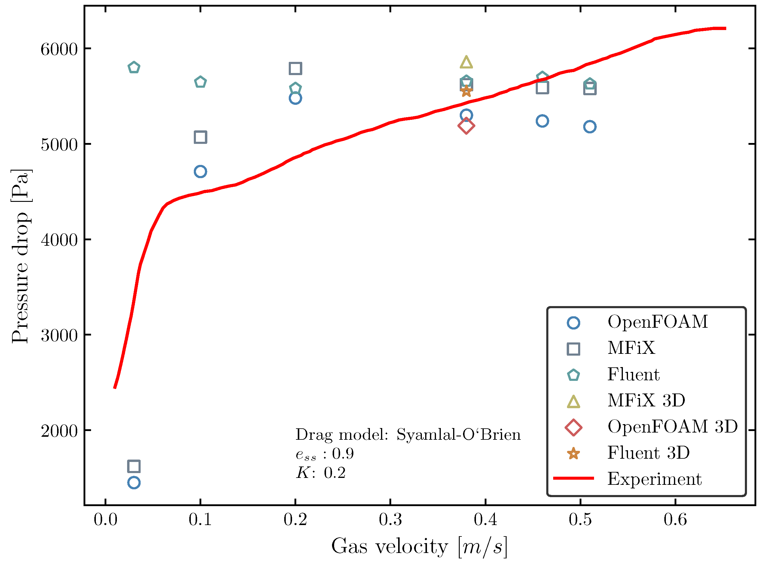
Figure 5.
Pressure drop for different superficial gas velocities with the Gidaspow drag model in ANSYS Fluent, MFiX and OpenFOAM. Experiment data were taken from [19], with permission from Elsevier.
Figure 5.
Pressure drop for different superficial gas velocities with the Gidaspow drag model in ANSYS Fluent, MFiX and OpenFOAM. Experiment data were taken from [19], with permission from Elsevier.
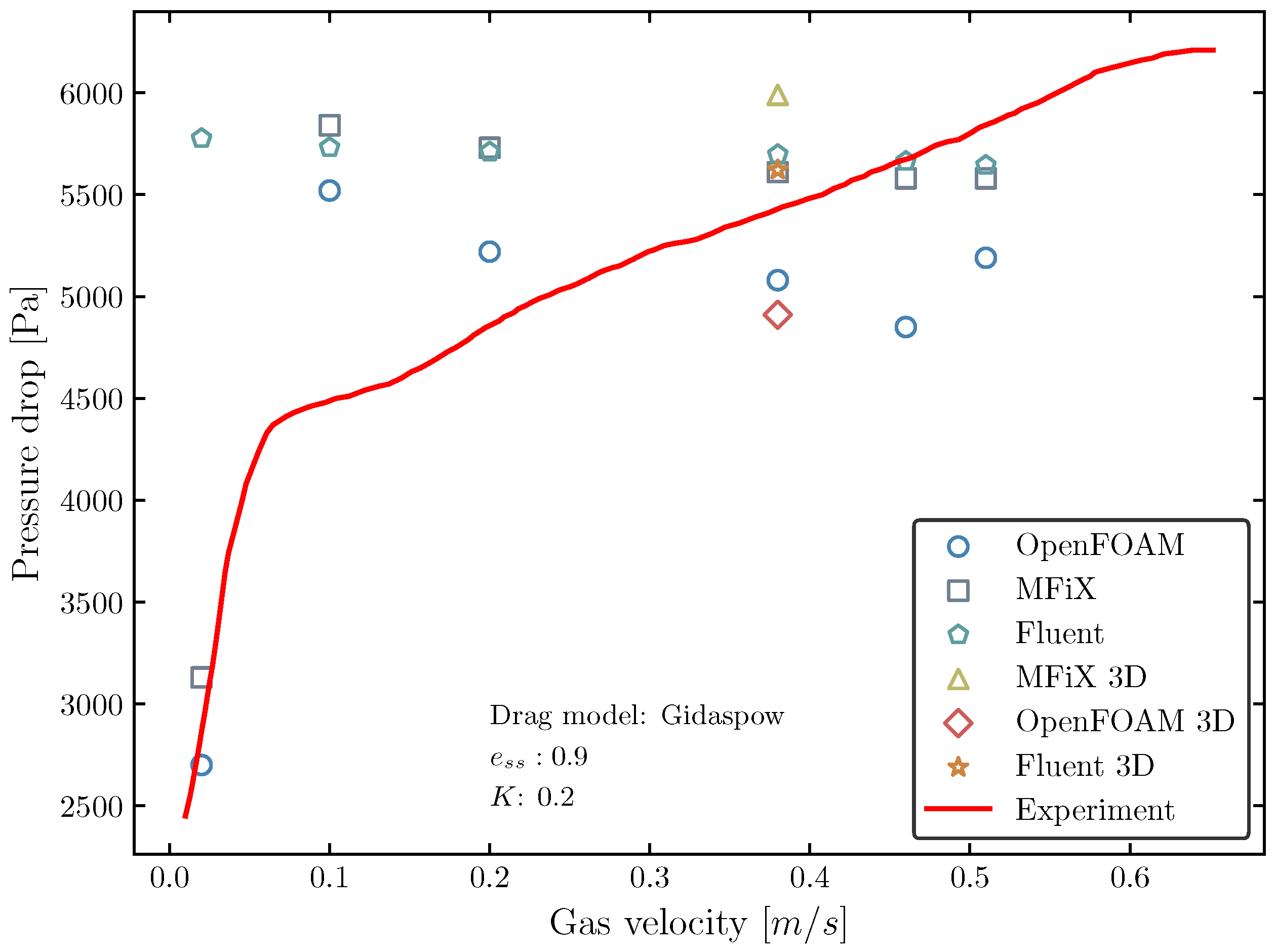
Figure 6.
Time-averaged solid velocities recorded between 3 to 12 seconds for a superficial gas velocity of 0.38 m/s with Syamlal-O`Brien drag model. These measurements were conducted at a height of y = 0.2 m.
Figure 6.
Time-averaged solid velocities recorded between 3 to 12 seconds for a superficial gas velocity of 0.38 m/s with Syamlal-O`Brien drag model. These measurements were conducted at a height of y = 0.2 m.
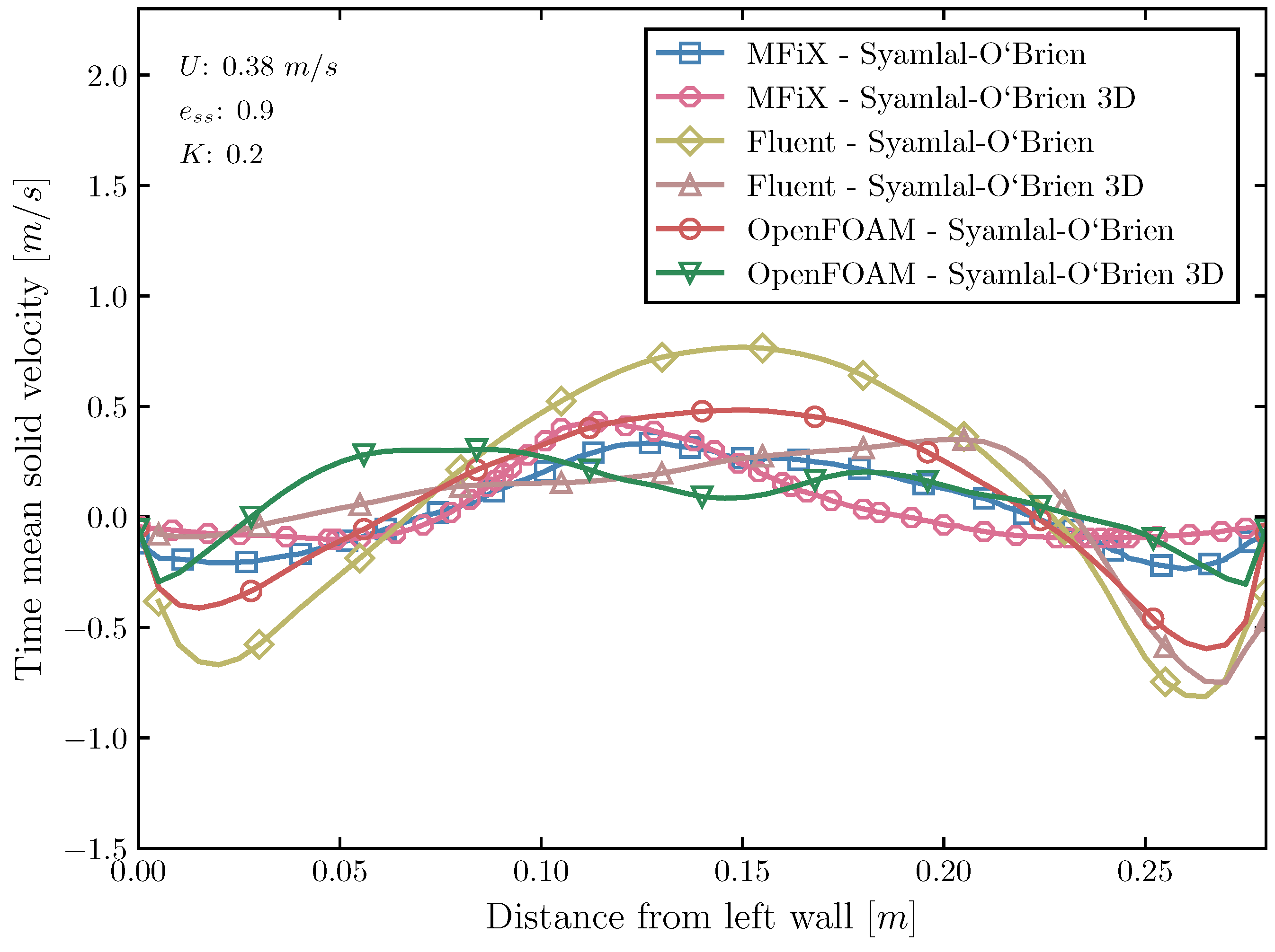
Figure 7.
Time-averaged solid velocities recorded between 3 to 12 seconds for a superficial gas velocity of 0.38 m/s with Gidaspow drag model. These measurements were conducted at a height of y = 0.2 m.
Figure 7.
Time-averaged solid velocities recorded between 3 to 12 seconds for a superficial gas velocity of 0.38 m/s with Gidaspow drag model. These measurements were conducted at a height of y = 0.2 m.
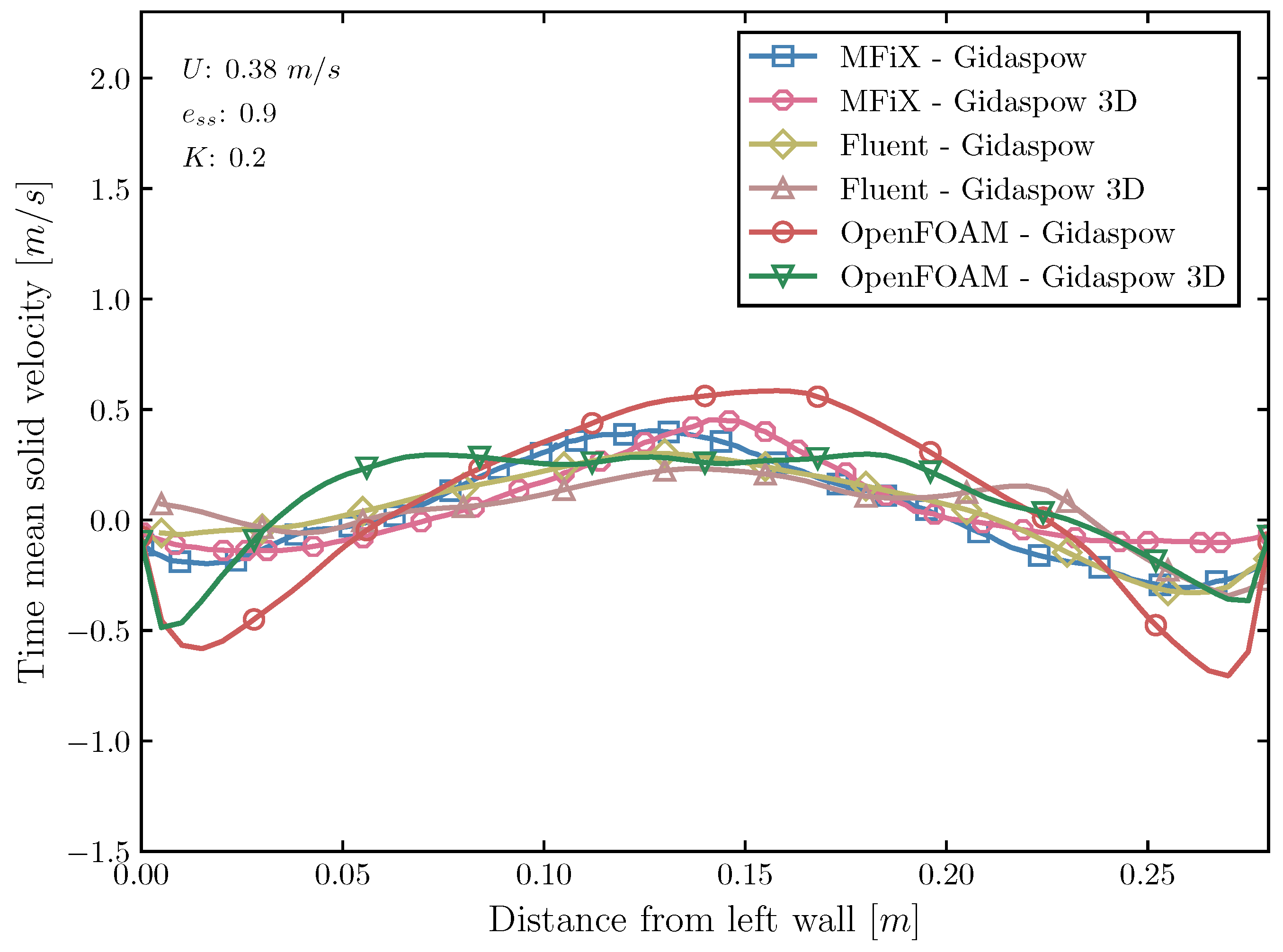
Figure 8.
Time-averaged voidage recorded between 3 to 12 seconds for a superficial gas velocity of 0.38 m/s with Syamlal-O`Brien drag model. These measurements were conducted at a height of y = 0.2 m. Experiment data were taken from [19], with permission from Elsevier.
Figure 8.
Time-averaged voidage recorded between 3 to 12 seconds for a superficial gas velocity of 0.38 m/s with Syamlal-O`Brien drag model. These measurements were conducted at a height of y = 0.2 m. Experiment data were taken from [19], with permission from Elsevier.
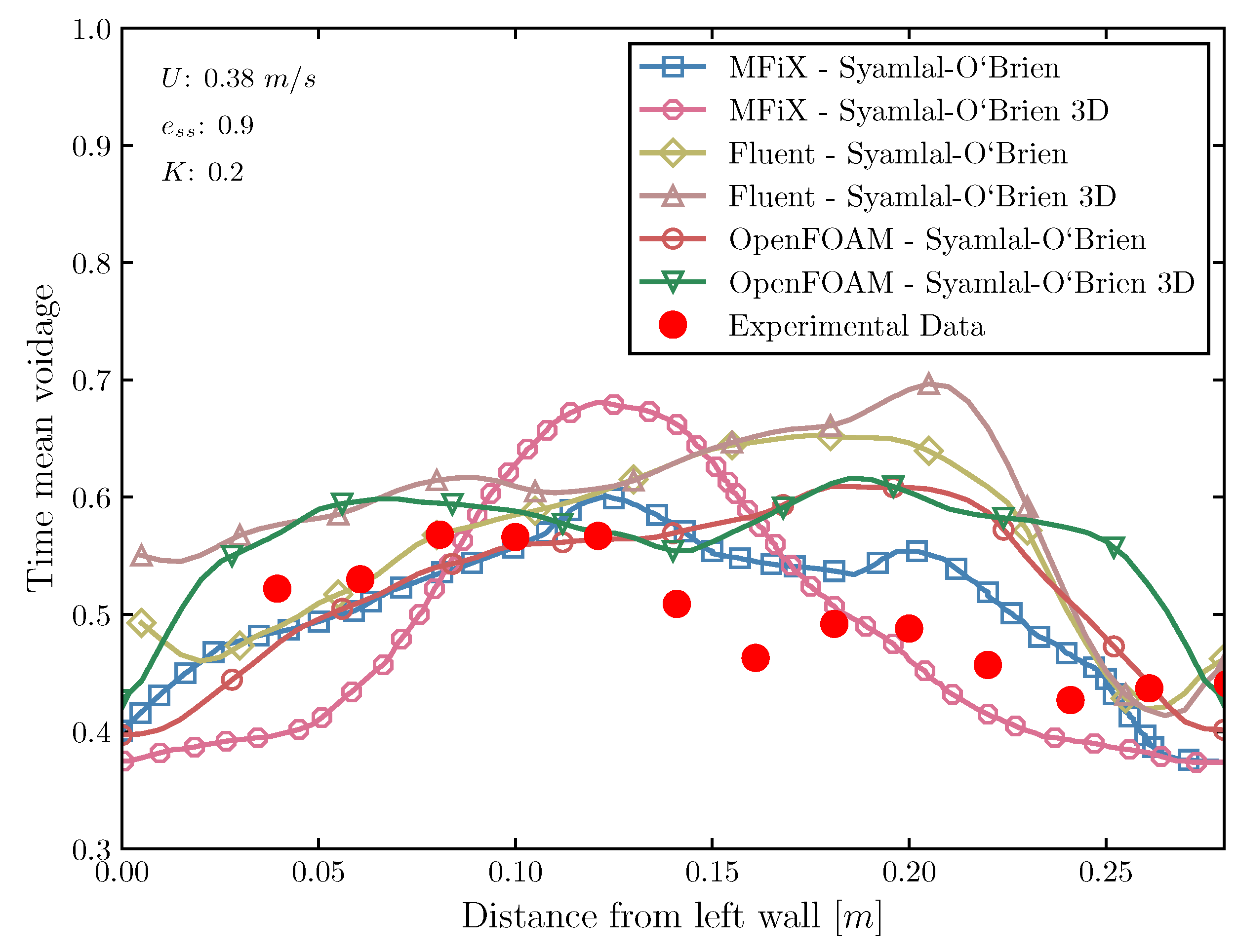
Figure 9.
Time-averaged voidage recorded between 3 to 12 seconds for a superficial gas velocity of 0.38 m/s with Gidaspow drag model. These measurements were conducted at a height of y = 0.2 m. Experiment data were taken from [19], with permission from Elsevier.
Figure 9.
Time-averaged voidage recorded between 3 to 12 seconds for a superficial gas velocity of 0.38 m/s with Gidaspow drag model. These measurements were conducted at a height of y = 0.2 m. Experiment data were taken from [19], with permission from Elsevier.
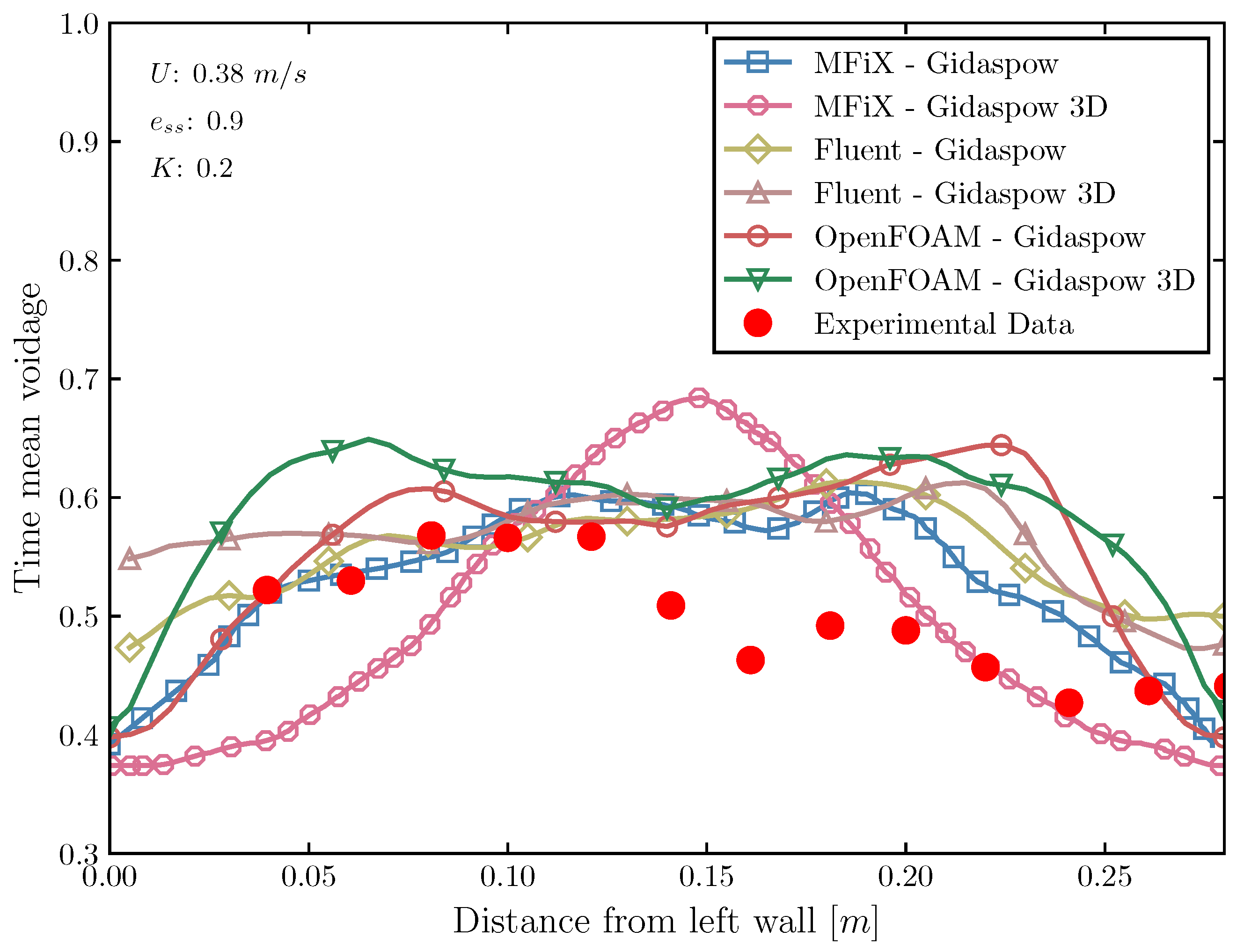
Figure 10.
Particles distribution throughout the simulation with the Syamlal-O`Brien drag model with various superficial gas velocities in ANSYS Fluent, MFiX and OpenFOAM.
Figure 10.
Particles distribution throughout the simulation with the Syamlal-O`Brien drag model with various superficial gas velocities in ANSYS Fluent, MFiX and OpenFOAM.
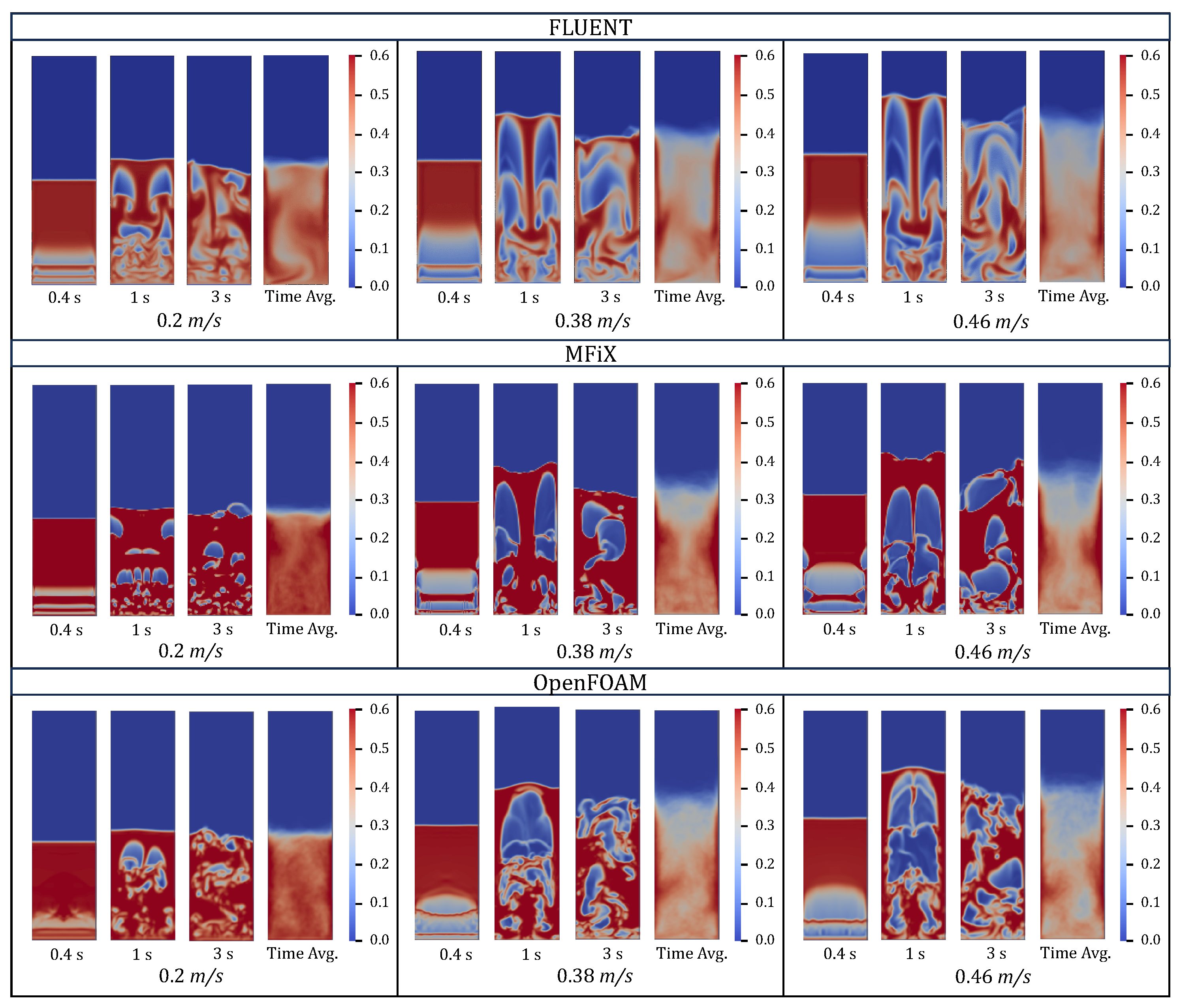
Figure 11.
Particles distribution throughout the simulation with the Gidaspow drag model with various superficial gas velocities in ANSYS Fluent, MFiX and OpenFOAM.
Figure 11.
Particles distribution throughout the simulation with the Gidaspow drag model with various superficial gas velocities in ANSYS Fluent, MFiX and OpenFOAM.
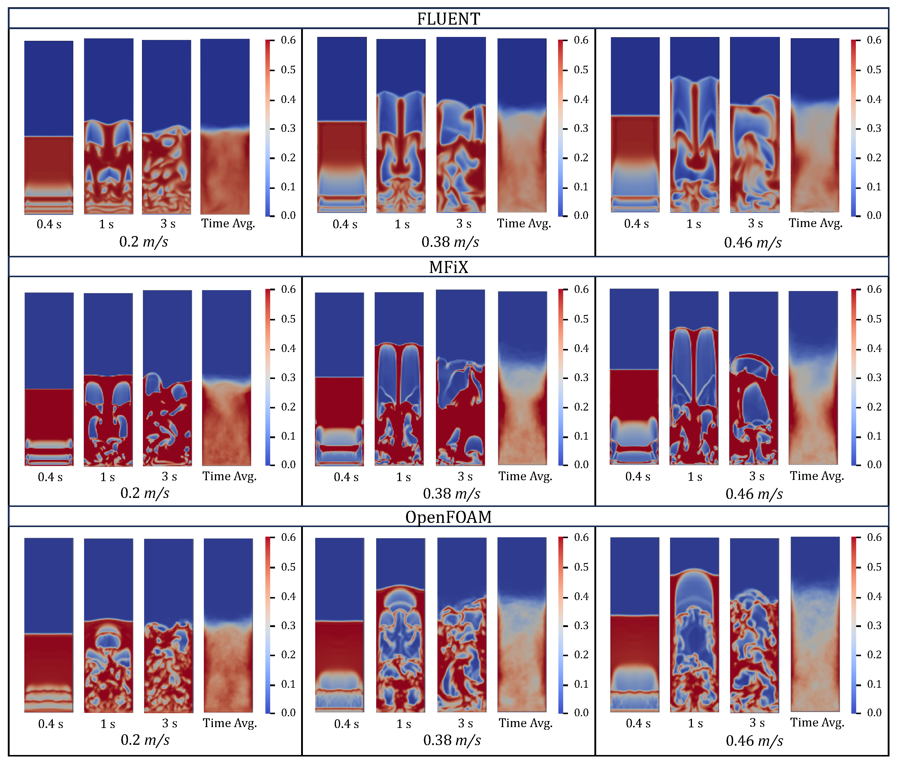
Figure 12.
Simulation Error based on experimental data of Taghipour et al. [19] at y = 0.2 and u = 0.38 m/s, with permission from Elsevier.
Figure 12.
Simulation Error based on experimental data of Taghipour et al. [19] at y = 0.2 and u = 0.38 m/s, with permission from Elsevier.
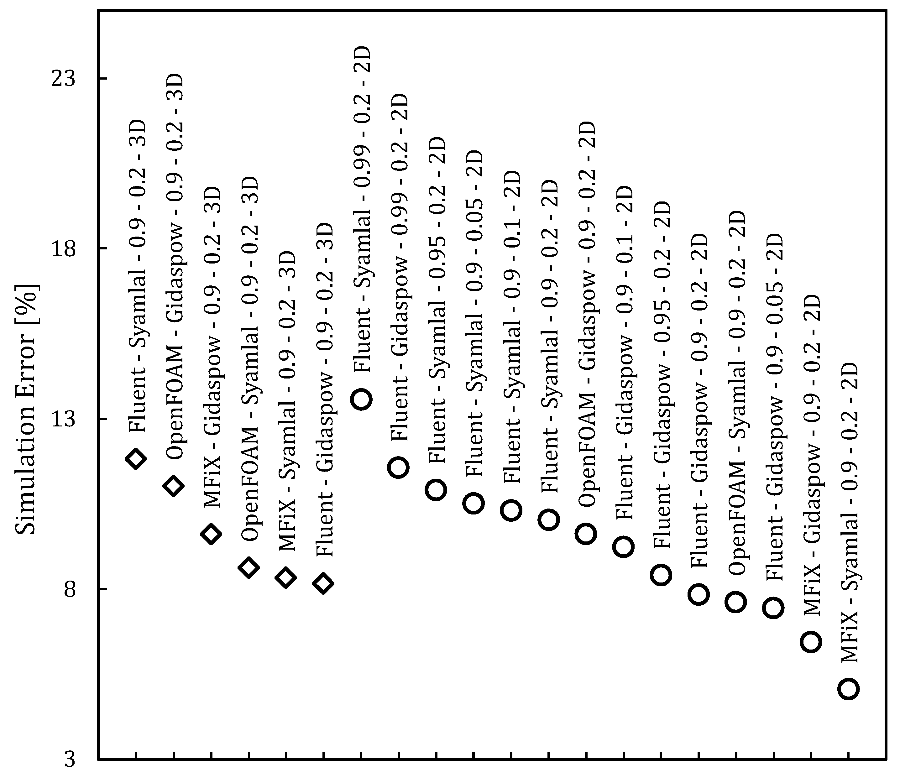
Table 1.
Parameters of simulation cases performed in this study, inspired from Taghipour et al. [19].
Table 1.
Parameters of simulation cases performed in this study, inspired from Taghipour et al. [19].
| Description | Value | Remark |
| Bed width | 0.28 m | Fixed value |
| Bed height | 1 m | Fixed value |
| Static bed height | 0.4 m | Fixed value |
| Grid interval spacing | 0.005 m | Specified |
| Particle density | 2500 kg/m | Glass beads |
| Gas density | 1.225 kg/m | Air |
| Gas kinematic viscosity | m/s | Fixed value |
| Mean particle diameter | 275 m | Uniformly distributed |
| Initial solids packing | 0.6 | Fixed value |
| Maximum solids packing | 0.63 | Fixed value |
| Superficial gas velocity | 0.03 - 0.51 m/s | Parametized |
| Restitution coefficient | 0.9; 0.95; 0.99 | Parametized |
| Specularity coefficient | 0.05; 0.1; 0.2 | Parametized |
| Min. fluidization velocity | 0.065 m/s | Experiment |
| Viscous model | Laminar | Specified |
| Drag model | Syamlal-O’Brien; Gidaspow | Parametized [5,20] |
| Granular bulk viscosity | Lun et al. | [25,26] |
| Kinetic viscosity | Syamlal-O’Brien; Gidaspow | Parametized |
| Granular temperature | Algebraic; PDE; PDE | ANSYS Fluent; OpenFOAM; MFiX |
| Frictional viscosity | Schaeffer | [25,27] |
| Frictional pressure | Based-ktgf | [25] |
| Radial distribution | Lun et al | [25,26] |
| Inlet boundary condition | Velocity | Superficial gas velocity |
| Outlet boundary condition | Outflow | Fully developed flow |
| Time steps | 0.001 s | Specified |
| Time averaged range | 3 - 12 s | Specified |
| Transient formulation | First order | Specified |
| Solution algorithm | SIMPLE; PIMPLE; MFiX algorithm | ANSYS Fluent; OpenFOAM; MFiX |
Table 2.
Parameters of simulation cases performed in this study.
| Case | Software | u, m/s | Drag force | K | Geomery | , Pa | ||
| 1 | Fluent | 0.03 | Syamlal-O’Brien | 0.9 | 0.2 | 2D | 0.975 | 5800* |
| 2 | Fluent | 0.1 | Syamlal-O’Brien | 0.9 | 0.2 | 2D | 1.162 | 5647 |
| 3 | Fluent | 0.2 | Syamlal-O’Brien | 0.9 | 0.2 | 2D | 1.388 | 5581 |
| 4 | Fluent | 0.38 | Syamlal-O’Brien | 0.9 | 0.2 | 2D | 1.700 | 5657 |
| 5 | Fluent | 0.46 | Syamlal-O’Brien | 0.9 | 0.2 | 2D | 1.875 | 5697 |
| 6 | Fluent | 0.51 | Syamlal-O’Brien | 0.9 | 0.2 | 2D | 1.963 | 5628 |
| 7 | Fluent | 0.38 | Syamlal-O’Brien | 0.95 | 0.2 | 2D | 1.762 | 5613 |
| 8 | Fluent | 0.38 | Syamlal-O’Brien | 0.99 | 0.2 | 2D | 1.813 | 5577 |
| 9 | Fluent | 0.38 | Syamlal-O’Brien | 0.9 | 0.05 | 2D | 1.700 | 5633 |
| 10 | Fluent | 0.38 | Syamlal-O’Brien | 0.9 | 0.1 | 2D | 1.700 | 5514 |
| 11 | Fluent | 0.38 | Syamlal-O’Brien | 0.9 | 0.2 | 3D | 1.513 | 5551 |
| 12 | Fluent | 0.03 | Gidaspow | 0.9 | 0.2 | 2D | 0.975 | 5776* |
| 13 | Fluent | 0.1 | Gidaspow | 0.9 | 0.2 | 2D | 1.087 | 5731 |
| 14 | Fluent | 0.2 | Gidaspow | 0.9 | 0.2 | 2D | 1.275 | 5710 |
| 15 | Fluent | 0.38 | Gidaspow | 0.9 | 0.2 | 2D | 1.563 | 5697 |
| 16 | Fluent | 0.46 | Gidaspow | 0.9 | 0.2 | 2D | 1.663 | 5663 |
| 17 | Fluent | 0.51 | Gidaspow | 0.9 | 0.2 | 2D | 1.762 | 5644 |
| 18 | Fluent | 0.38 | Gidaspow | 0.95 | 0.2 | 2D | 1.550 | 5608 |
| 19 | Fluent | 0.38 | Gidaspow | 0.99 | 0.2 | 2D | 1.625 | 5661 |
| 20 | Fluent | 0.38 | Gidaspow | 0.9 | 0.05 | 2D | 1.525 | 5554 |
| 21 | Fluent | 0.38 | Gidaspow | 0.9 | 0.1 | 2D | 1.539 | 5604 |
| 22 | Fluent | 0.38 | Gidaspow | 0.9 | 0.2 | 3D | 1.625 | 5622 |
| 23 | OpenFOAM | 0.03 | Syamlal-O’Brien | 0.9 | 0.2 | 2D | 1.000 | 1450 |
| 24 | OpenFOAM | 0.1 | Syamlal-O’Brien | 0.9 | 0.2 | 2D | 1.020 | 4710 |
| 25 | OpenFOAM | 0.2 | Syamlal-O’Brien | 0.9 | 0.2 | 2D | 1.260 | 5480 |
| 26 | OpenFOAM | 0.38 | Syamlal-O’Brien | 0.9 | 0.2 | 2D | 1.630 | 5300 |
| 27 | OpenFOAM | 0.46 | Syamlal-O’Brien | 0.9 | 0.2 | 2D | 1.800 | 5240 |
| 28 | OpenFOAM | 0.51 | Syamlal-O’Brien | 0.9 | 0.2 | 2D | 1.860 | 5180 |
| 29 | OpenFOAM | 0.38 | Syamlal-O’Brien | 0.9 | 0.2 | 3D | 1.520 | 5190 |
| 30 | OpenFOAM | 0.03 | Gidaspow | 0.9 | 0.2 | 2D | 1.000 | 2700 |
| 31 | OpenFOAM | 0.1 | Gidaspow | 0.9 | 0.2 | 2D | 1.160 | 5520 |
| 32 | OpenFOAM | 0.2 | Gidaspow | 0.9 | 0.2 | 2D | 1.350 | 5220 |
| 33 | OpenFOAM | 0.38 | Gidaspow | 0.9 | 0.2 | 2D | 1.720 | 5080 |
| 34 | OpenFOAM | 0.46 | Gidaspow | 0.9 | 0.2 | 2D | 1.890 | 4850 |
| 35 | OpenFOAM | 0.51 | Gidaspow | 0.9 | 0.2 | 2D | 1.980 | 5190 |
| 36 | OpenFOAM | 0.38 | Gidaspow | 0.9 | 0.2 | 3D | 1.520 | 4910 |
| 37 | MFiX | 0.03 | Syamlal-O’Brien | 0.9 | 0.2 | 2D | 0.951 | 1620 |
| 38 | MFiX | 0.1 | Syamlal-O’Brien | 0.9 | 0.2 | 2D | 1.040 | 5070 |
| 39 | MFiX | 0.2 | Syamlal-O’Brien | 0.9 | 0.2 | 2D | 1.200 | 5790 |
| 40 | MFiX | 0.38 | Syamlal-O’Brien | 0.9 | 0.2 | 2D | 1.520 | 5620 |
| 41 | MFiX | 0.46 | Syamlal-O’Brien | 0.9 | 0.2 | 2D | 1.700 | 5590 |
| 42 | MFiX | 0.51 | Syamlal-O’Brien | 0.9 | 0.2 | 2D | 1.790 | 5580 |
| 43 | MFiX | 0.38 | Syamlal-O’Brien | 0.9 | 0.2 | 3D | 1.460 | 5860 |
| 44 | MFiX | 0.03 | Gidaspow | 0.9 | 0.2 | 2D | 0.947 | 3130 |
| 45 | MFiX | 0.1 | Gidaspow | 0.9 | 0.2 | 2D | 1.080 | 5840 |
| 46 | MFiX | 0.2 | Gidaspow | 0.9 | 0.2 | 2D | 1.310 | 5730 |
| 47 | MFiX | 0.38 | Gidaspow | 0.9 | 0.2 | 2D | 1.640 | 5610 |
| 48 | MFiX | 0.46 | Gidaspow | 0.9 | 0.2 | 2D | 1.730 | 5580 |
| 49 | MFiX | 0.51 | Gidaspow | 0.9 | 0.2 | 2D | 1.910 | 5580 |
| 50 | MFiX | 0.38 | Gidaspow | 0.9 | 0.2 | 3D | 1.460 | 5990 |
Disclaimer/Publisher’s Note: The statements, opinions and data contained in all publications are solely those of the individual author(s) and contributor(s) and not of MDPI and/or the editor(s). MDPI and/or the editor(s) disclaim responsibility for any injury to people or property resulting from any ideas, methods, instructions or products referred to in the content. |
© 2024 by the authors. Licensee MDPI, Basel, Switzerland. This article is an open access article distributed under the terms and conditions of the Creative Commons Attribution (CC BY) license (http://creativecommons.org/licenses/by/4.0/).
Copyright: This open access article is published under a Creative Commons CC BY 4.0 license, which permit the free download, distribution, and reuse, provided that the author and preprint are cited in any reuse.


