
Submitted:
20 May 2024
Posted:
22 May 2024
Read the latest preprint version here
Abstract
Principal Component Analysis (PCA) is a method that identifies common directions within multivariate data and presents the data in as few dimensions as possible. One of the advantages of PCA is its objectivity, as the same results can be obtained regardless of who performs the analysis. However, PCA is not a robust method and is sensitive to noise. Consequently, the directions identified by PCA may deviate slightly. If we can teach PCA to account for this deviation and correct it, the results should become more comprehensible. The methods for doing this and an issue with this are presented.
Keywords:
Principal Component Analysis
; rotation matrix
; adjusting
; unitary matrix
Introduction
Much of the data we handle consists of numerous measurement items, necessitating multivariate analysis. While several methods are known, Principal Component Analysis (PCA) is particularly suitable for scientific analysis due to its limited options and high reproducibility [1,2,3,4,5,6,7,8,9,10]. In PCA, we use Singular Value Decomposition (SVD) to separate the matrix into unitary matrices (U and V) and a diagonal matrix (D): M = UDV*, where V* denotes the conjugate transpose of V and M is the data to be analysed, often centred or even scaled. The diagonal elements of D are sorted. The principal components (PCs) can then be obtained from these as follows: PCs = MV = UD, PCi = M*U = VD, where the column vector of PCs are those for samples and those of PCi are for items (PC1, PC2, etc.) [4]. Since U and V are unitary matrices, with properties such as (U*U = I) and (U U* = I), these row and column vectors are independent, and their Euclidean distances are all 1: those column or row vectors have length 1 because taking the inner product with itself = sum of squares of the elements gives 1, and taking the inner product with others gives zero, showing that each of them is orthogonal to the other. The resulting PCi or PCs column vectors are also independent. They can be interpreted as rotations of the original matrix M or as axes given by the unitary matrices with lengths determined by D. Since D is sorted, PC1, PC2, in that order, cover a larger percentage of the data scatter. Thus, PCA finds common directions in M and summarizes them in the order of their length of the direction. The advantage of PCA is that it can thus compress the many dimensions of multivariate data as much as possible.
However, one of the drawbacks of PCA is its lack of robustness. Even a single outlier can cause errors in SVD. Naturally, noise affects the results. It’s common for the identified directions to be slightly off. For instance, group positions or individual PCi values may deviate slightly from the axes due to rotation. Since experimental data inherently contains noise, it is expected that noise-sensitive PCA will exhibit such errors. In such situations, there may be a temptation to adjust PCA results or train PCA to correct rotations. In this context, I discuss potential correction methods and raise associated issues.
Materials and Methods
The data used in this study was obtained from student internships on soil study. All calculations were performed using R [11], and both the data and R code are provided as supplementary material. Due to significant variability in calcium data, the data was z-normalized for each item before applying SVD. Consequently, the centring point corresponds to the mean value of the data; these centring and scaling steps are among the few options available in PCA. The calculation method for PCA is as described in the introduction. Additionally, since the number of measured items and the sample size differ considerably, I scaled the PCs by the square root of the sample size to facilitate biplots on a common axis [4]. Specifically, , where ni is number of items, and so on.
Results
An example of a slight deviation of PCi from the axes can be seen in Figure 1, which represents PCA of data obtained from measuring substances in soil. Samples P1 to P4 were collected from points downwards at 50 cm intervals from the surface of the padding field. Overall, soluble Na, K, and Mg appear to have infiltrated the soil, while less soluble Ca remains near the surface. In unfertilized forest areas, these materials are notably less. The measured items effectively differentiate these samples; this data demonstrates the impact of human activity on the land—increased calcium levels may alter surface soil, and cations that have penetrated underground could contribute to salinity. However, upon closer examination, the figure appears to be rotated counter clockwise by 14 degrees.
For example, when creating a two-dimensional plot using PC1 and PC2 for a matrix of four columns, these two column vectors can be rotated by taking the inner product of them with a rotation matrix:
This is almost the identity matrix, but alteration was made at the upper left. This rotation matrix is unitary, so , where I is the identity matrix. Consequently, if we rotate two columns of U, the adjusted U is. The resulting rotated matrix Ua is also unitary, as . Since U and V are related as mirror images, if we rotate one column vector, we need to rotate the corresponding column vector by the same amount. From M = UDV*, we have . The matrix that is sandwiched by the two unitary matrixes, , is not necessarily a diagonal matrix, according to the twice rotations of D. By using Da, PCsa = PCsR(θ) = MVa=UaDa and PCia = PCiR(θ) = M*Ua =VaDa. Hence the resulting column vectors of PCsa and PCia are not necessarily independent. The degree of dependence depends on the rotation angle.
The actual result after rotating by 14 degrees is shown in Figure 2. Each item is now displayed closer to the axes. Notably, the high calcium content in P1 and P2, as well as the abundance of soluble cations in G4 and P4, is more clearly visible. The question now is how much independence has been compromised. This becomes evident when examining the contribution of PC1.
Often, contributions are derived from the diagonal elements of D. As D is a diagonal matrix, the contributions can be obtained from the components diag(D)/Σ(D). However, since Da is not diagonal, we need to calculate the Euclidean distance using the squared sum of each column vector. The contribution is then given by the distance / total distance.
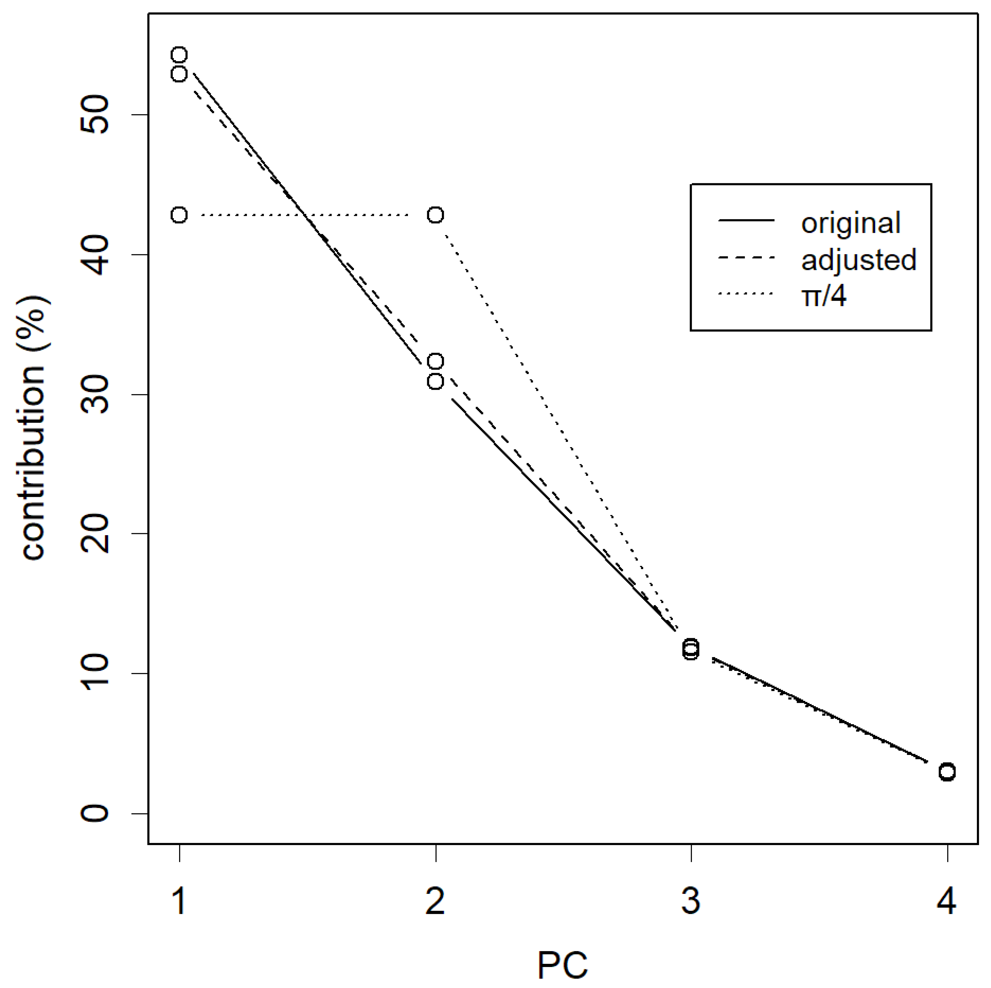
From the perspective of PCA, the goal is to collect contributions primarily from the top PCs. In the case of rotating by 14 degrees, the loss appears to be relatively small (Figure 3, dashed line). By the way, the most significant change occurs when rotating by 45 degrees, π/4 (dotted line). At this point, PC1 completely loses its advantage over PC2, and both have equal contributions. And of course, if rotated by 90 degrees, PC1 and PC2 would effectively swap places, and their contributions would naturally exchange as well. As the data’s dispersion remains preserved, the sum of all total distance is maintained regardless of the degree of rotations.
Discussion
The results of the rotated PCA, albeit by a small angle, were more comprehensible. This somewhat compromises the priority of higher levels of PCs, but if the angle is not too large, the damage will not be too great. Understanding PCA plots can often be challenging, as PCA merely provides a summary, without revealing the specifics. Interpretation of the plot is left to the analyst. In this regard, enhanced readability could be highly appreciated. Notably, PCA is sensitive to noise. If this effect can be easily mitigated, it’s worth considering. This somewhat compromises the priority of higher levels of PCs, but if the angle is not too large, the damage will not be too great.
However, this constitutes an active intervention by the analyst, potentially compromising PCA’s objectivity. The beauty of PCA lies in its impartiality. Diluting this aspect would be regrettable and might even lead to data manipulation. If such adjustments are made, it’s essential to keep the original, unadjusted plot available. Alternatively, the rotated plot could serve as supplementary material for explaining the results.
References
- Jackson, E. A Use's Guide to Principal Components; Wiley 1991.
- Jolliffe, I.T. Principal Component Analysis; Springer: 2002.
- Ringnér, M. What is principal component analysis? Nat Biotechnol 2008, 26, 303-304. [CrossRef] [PubMed]
- Konishi, T. Principal component analysis for designed experiments. BMC Bioinformatics 2015, 16, S7. [CrossRef] [PubMed]
- Bartholomew, D.J. Principal Components Analysis. In International Encyclopedia of Education (Third Edition), Peterson, P., Baker, E., McGaw, B., Eds.; Elsevier: Oxford, 2010; pp. 374-377.
- Raychaudhuri, S.; Stuart, J.M.; Altman, R.B. Principal components analysis to summarize microarray experiments: application to sporulation time series. Pac Symp Biocomput 2000, 455-466. [CrossRef] [PubMed]
- Xin, T.; Che, L.; Xi, C.; Singh, A.; Nie, X.; Li, J.; Dong, Y.; Lu, D. Experimental Quantum Principal Component Analysis via Parametrized Quantum Circuits. Physical Review Letters 2021, 126, 110502. [CrossRef] [PubMed]
- Medea, B.; Karapanagiotidis, T.; Konishi, M.; Ottaviani, C.; Margulies, D.; Bernasconi, A.; Bernasconi, N.; Bernhardt, B.C.; Jefferies, E.; Smallwood, J. How do we decide what to do? Resting-state connectivity patterns and components of self-generated thought linked to the development of more concrete personal goals. Experimental Brain Research 2018, 236, 2469-2481. [CrossRef] [PubMed]
- Abdi, H.; Williams, L.J. Principal component analysis. WIREs Computational Statistics 2010, 2, 433-459. [CrossRef]
- Jolliffe, I.T.; Cadima, J. Principal component analysis: a review and recent developments. Philosophical Transactions of the Royal Society A: Mathematical, Physical and Engineering Sciences 2016, 374, 20150202. [CrossRef] [PubMed]
- R Core Team. R: A Language and Environment for Statistical Computing.; R Foundation for Statistical Computing: Vienna, Austria, 2024.
Figure 1.
Results of material quantity measurements from soil material. Soil samples were obtained from rice padding field, grove soil of dry farmland and forest. The black and blue biplots show the PC of the samples, PCs, and the PC of the items, PCi, respectively. Soluble cations and water-insoluble Ca guided PC1 and PC2, respectively.
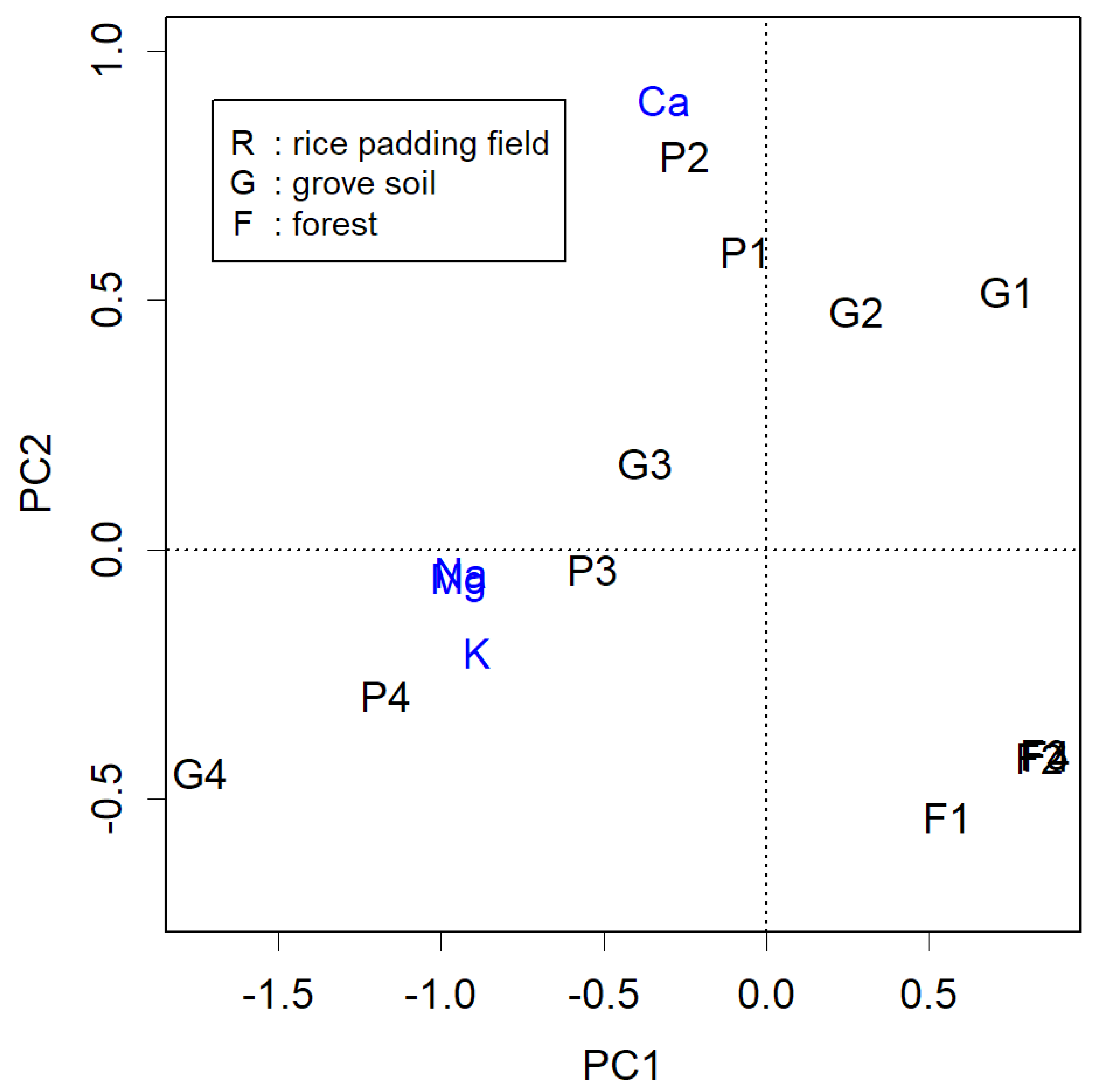
Figure 2.
Adjusted results from Figure 1 by rotating the plot by 14° clockwise. Each PCi is more along the axis, with the characteristic G4 and P4 in PC1 of the PCs, and the characteristic P1 and P2 in PC2 also appearing more along their respective axes.
Figure 2.
Adjusted results from Figure 1 by rotating the plot by 14° clockwise. Each PCi is more along the axis, with the characteristic G4 and P4 in PC1 of the PCs, and the characteristic P1 and P2 in PC2 also appearing more along their respective axes.
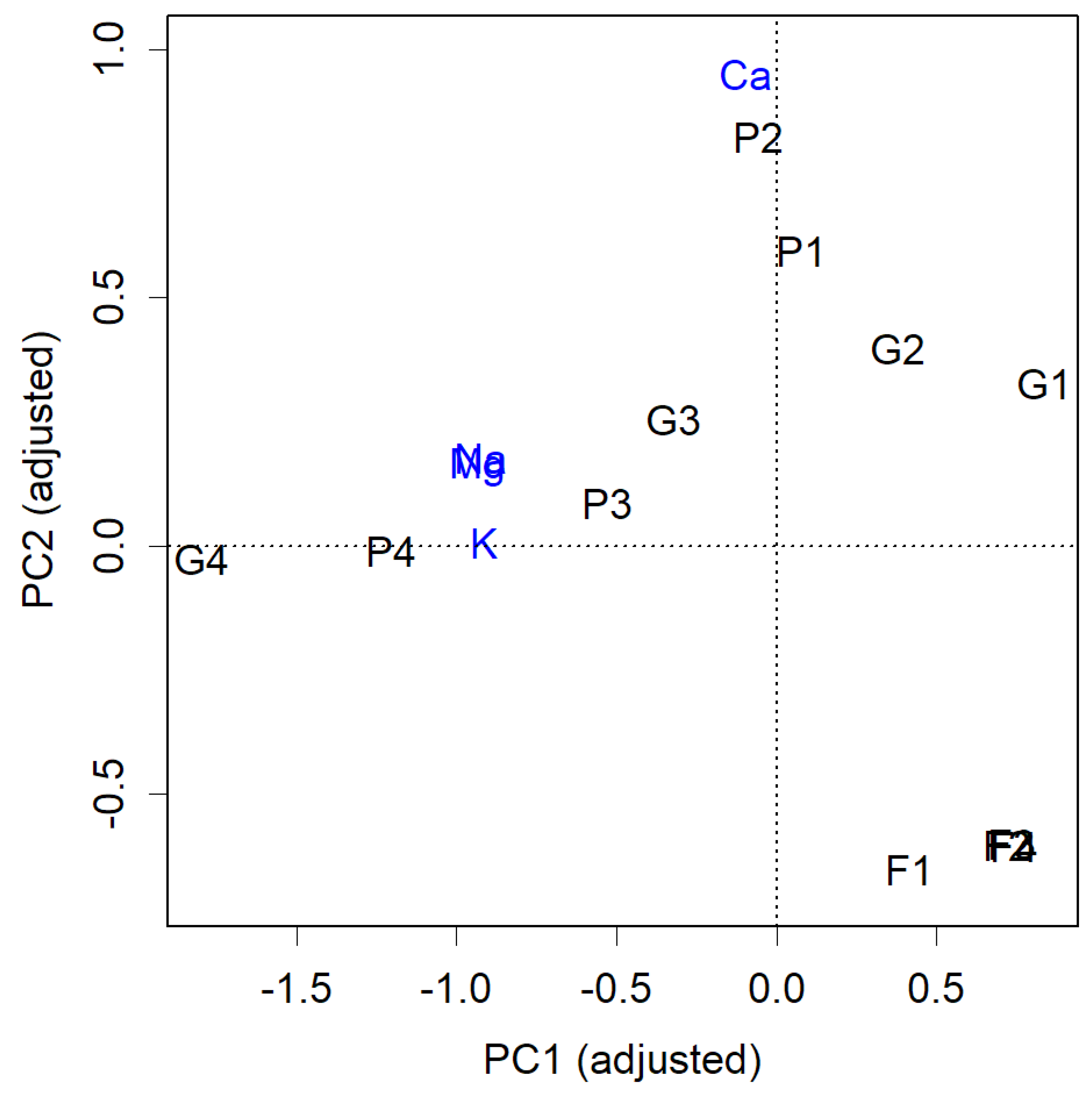
Figure 3.
Contribution of each method. The original PCA is the most ideal diagram, with the greatest concentration on PC1; adjusting by 14° rotation weakens this concentration somewhat; rotating by 45°, 4/π, the advantage of PC1 disappears and becomes the same contribution as that of PC2. Rotation by 90 degrees, not shown here, replaces PC1 and PC2.
Disclaimer/Publisher’s Note: The statements, opinions and data contained in all publications are solely those of the individual author(s) and contributor(s) and not of MDPI and/or the editor(s). MDPI and/or the editor(s) disclaim responsibility for any injury to people or property resulting from any ideas, methods, instructions or products referred to in the content. |
© 2024 by the authors. Licensee MDPI, Basel, Switzerland. This article is an open access article distributed under the terms and conditions of the Creative Commons Attribution (CC BY) license (http://creativecommons.org/licenses/by/4.0/).
Copyright: This open access article is published under a Creative Commons CC BY 4.0 license, which permit the free download, distribution, and reuse, provided that the author and preprint are cited in any reuse.


