Submitted:
14 May 2024
Posted:
14 May 2024
You are already at the latest version
Abstract
The next-generation communication systems demand integration of sensing, communication, and power transfer (PT) capabilities, requiring high spectral efficiency, energy efficiency, and low cost, while also necessitating robustness in high-speed scenarios. Integrated sensing and communication systems (ISACS) exhibit the ability to simultaneously perform communication and sensing tasks using a single RF signal, while simultaneous wireless information and power transfer (SWIPT) systems can handle simultaneous information and energy transmission, and orthogonal time frequency space (OTFS) signals are adept at handling high Doppler scenarios. Combining the advantages of these three technologies, a novel cyclic prefix (CP) OTFS based integrated simultaneous wireless sensing, communication, and power transfer system (ISWSCPTS) framework is proposed in this work. Within the ISWSCPTS, the CP-OTFS matched filter (MF) based target detection and parameters estimation (MF-TDaPE) algorithm is proposed to endow the system with sensing capabilities. To enhance the system’s sensing capability, a waveform design algorithm based on CP-OTFS ambiguity function shaping (AFS) is proposed, which is solved by iteratively method. Furthermore, to maximize the system’s sensing performance under communication and PT Quality of Service (QoS) constraints, a semidefinite relaxation (SDR) beamforming design (SDR-BD) algorithm is proposed, solved using through SDR technique. Simulation results demonstrate that the ISWSCPTS exhibits stronger parameter estimation performance in high-speed scenarios compared to orthogonal frequency division multiplexing (OFDM), waveform designed by CP-OTFS AFS demonstrates superior interference resilience, and beamforming designed by SDR-BD strikes a balance in the overall performance of the ISWSCPTS.
Keywords:
simultaneous wireless information and power transfer (SWIPT)
; integrated sensing and communication systems (ISACS)
; orthogonal time frequency space (OTFS)
; waveform design
; beamforming
; semidefinite relaxation (SDR)
; matched filter (MF)
1. Introduction
The next-generation communication systems require the integration of additional functionalities to enhance system spectral efficiency, energy efficiency, and reduce system costs. Integrated sensing and communication systems (ISACS), which converge sensing and communication functionalities within a unified framework, have gained significant traction in recent years [1,2,3,4]. By co-locating sensing and communication tasks and sharing common resources such as antennas and signal processing algorithms, ISACS promise enhanced performance, reduced latency, and improved resource utilization compared to traditional separate implementations. However, the functionalities of ISACS systems still do not fully leverage the potential of wireless radio frequency signals, such as power transfer (PT).
Certain modern wireless applications impose energy transfer requirements on ISACS systems. One such example is battlefield unmanned aerial vehicle (UAV). In combat environments, UAVs operating under constrained resources need to simultaneously accomplish target perception, information transmission, and enhance endurance. One approach to addressing this challenge is the efficient and rational allocation of power in ISACS systems to improve energy efficiency. Some existing works have studied power allocation problems in ISACS systems. Another approach is equipping ISACS with energy harvesting devices to collect energy from received radio frequency (RF) signals, thereby extending the system’s operational lifespan. Regarding the latter, simultaneous wireless information and power transfer (SWIPT), first proposed in [5], has garnered significant attention in recent years [6,7,8]. The core of SWIPT is to use a single signal as a carrier for both information transmission and energy transfer. Communication nodes extract information from the received signal, while energy harvesting nodes collect energy from it. Clearly, inspired by ISACS, SWIPT still has the potential to expand perception capabilities and further improve system efficiency.
In ISACS, the transmitted waveform plays a crucial role in determining system performance. The waveforms based on orthogonal frequency-division multiplexing (OFDM) is a promising choice due to its simple processing framework and high processing gain. However, the performance of OFDM-based waveforms sharply deteriorates in high-speed mobile scenarios [9]. Next-generation communication systems also demand robustness in high-Doppler time-varying scenarios, as required for ISACS. Orthogonal Time Frequency Space (OTFS), a modulation scheme that modulates/demodulates information in the Doppler-delay (DD) domain, has been proposed in recent years [10,11,12]. OTFS represents high-Doppler time-varying channels sparsely in the DD domain. Previous studies have shown that OTFS offers significant communication performance improvement compared to OFDM in high-speed time-varying scenarios [11,12]. OTFS is also utilized in sensing systems and demonstrates excellent performance compared to OFDM [9,13,14]. Due to the aforementioned advantages, cyclic prefix OTFS (CP-OTFS) is adopted as the fundamental waveform in this work.
Currently, there is relatively limited research on the integration of ISACS with SWIPT. In [15], the Cramer-Rao lower bound (CRLB) of the estimation of the targets’ angle is employed as the optimization objective, the beamforming is designed with communication and power transfer quality of service (QoS) constraints in mind. In this work, we propose a framework for cyclic prefix (CP)-OTFS based integrated simultaneous wireless sensing, communication, and power transfer system (ISWSCPTS) that incorporates both search mode (SM) and joint work mode (JWM). This framework integrates the advantages of ISACS and SWIPT, enabling simultaneous perception of targets, information transmission, and energy transfer capabilities. The main contributions of this work are as follows:
- The framework of ISWSCPTS is proposed. This framework comprises two operational modes: SM and JWM. To enhance sensing capabilities for both SM and JWM, The CP-OTFS matched filter (MF) based target detection and parameters estimation (MF-TDaPE) algorithm is proposed. This algorithm exhibits superior performance to OFDM in high-speed scenarios.
- An CP-OTFS ambiguity function (AF) shaping (AFS) waveform design algorithm is proposed. Firstly, a novel DD domain AF for CP-OTFS is proposed. Subsequently, aiming to minimize the integrated sidelobe level (ISL) of the proposed AF while adhering to the QoS for communication and PT and constant modulus constraints, a non-convex CP-OTFS waveform design optimization problem is formulated. This problem is then solved through an iterative algorithm to obtain waveforms with superior AF characteristics and interference resilience.
- The semidefinite relaxation (SDR) beamforming design (SDR-BD) algorithm tailored for ISWSCPTS is proposed. Initially, a non-convex optimization problem is formulated with sensing QoS as the optimization objective and communication and PT QoS as constraints. Subsequently, the SDR technique is employed to solve this problem. The designed waveform optimizes perceptual capability while ensuring communication and PT performance.
The structure of the paper is outlined as follows: Section 2.1 introduces the principles of CP-OTFS. Section 2.2 elaborates on the framework principles, waveform design, and beamforming design. Section 3 presents simulation results and corresponding discussions. Finally, Section 4 concludes with a summary and outlines future work prospects.
2. Materials and Methods
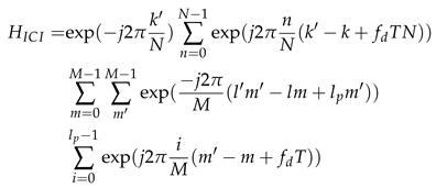
Considering an CP-OTFS based ISWSCPTS equipped with a uniform linear array (ULA) with transmitting elements and a single receiving antenna to sense a single target, deliver information to a single communication node (CN), and transfer energy to a single energy receiving node (ERN). As shown in Figure 1. The ISWSCPTS transmits a single information-carrying CP-OTFS signal. Through this multifunctional signal, the ISWSCPTS receives the target echo to complete perception, the CN receives the signal to accomplish information collection, and the ERN receives the signal to complete energy harvesting. The ISWSCPTS is also referred to as sensing node (SN) due to its function of sensing. We details the system model of ISWSCPTS starting from the CP-OTFS model.
2.1. The CP-OTFS Model
2.1.1. Basic Concepts of CP-OTFS
The time–frequency (TF) plane is discretized to a grid as following:
where T and are sampling intervals of time and frequency axes, respectively.
The modulated TF samples are transmitted over an OTFS frame with duration and occupy a bandwidth . The sampling frequency .
The DD plane is discretized to an lattice as following:
2.1.2. Input-Output Relationship of CP-OTFS Based ISWSCPTS
A. The transmitter model
The CP-OTFS based system is depicted in Figure 2. The symbols in DD domain is first transformed into symbols in TF domain by the inverse symplectic finite Fourier transform (ISFFT). Then, the Heisenberg transform is applied to to generate time domain discrete signal . The expression of is
where the is the transmitting rectangular pulse and its expression is
Next, the discrete CP-OTFS transmitting signal is constructed by adding a CP of length M to . Finally, is converted to radio frequency (RF) signal by RF transmitter module.
B. The channel model
In the application scenarios of ISWSCPTS, the perception target, communication channel, and energy transmission channel can all be modeled using a unified framework based on the DD channel (DDC) model. Assuming there are P DDCs which can be expressed as:
where is the channel gain coefficient, is the Doppler, and is the delay. Let .
In this work, we make the following assumptions:
where and are integers.
Thus, the discrete form of can be expressed as:
where
C. The receiver model
The received signal is transformed into the discrete-time signal by RF receiver module and removing the CP. can be expressed as:
where denotes modulo operation, is the additive Gaussian white noise (AWGN).
is converted to received symbols in TF domain through the Wigner transform. can be expressed as:
where is the receiving rectangular pulse and its expression is
Finally, is converted into the received symbols in DD domain through the symplectic finite Fourier transform (SFFT). can be expressed as:
where is AWGN matrix.
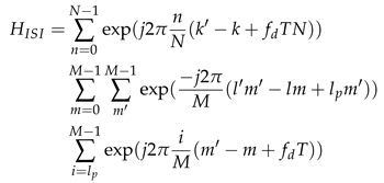
According to (13), each receiving symbol is the result of summing all input symbols weighted by . Clearly, is related to variables l, l, , and . The magnitude response of is as follows:
2.2. Framework of CP-OTFS Based ISWSCPTS
ISWSCPTS encompasses two work modes: SM JWM for perception, communication, and PT. The following provides a detailed description of these two modes.
2.2.1. The SM of ISWSCPTS
In the SM, ISWSCPTS lacks a priori information of DDCs for the target, communication, and power transfer, necessitating estimation of these parameters. In this mode, the ISWSCPTS scans the region of interest in a phased-array manner to acquire states of DDCs from various angles.
The TF-domain received target echo whose angle is the same as the searching direction can be expressed as:
where is the transmitting power, is the target scattering coefficient (TSC), is the TF-domain transmitting signal in search mode, is the AWGN matrix with the variance of each entry being , is the angle of the target, is the steering vector and can be expressed as:
where d is the antenna spacing, represents the wavelength.
In the phased-array manner, , thus (22) can be reformulated as:
According to (18), the vector form of DD-domain echo can be expressed as:
where , , vectorizes matrix along the row direction. For a target with delay tap and Doppler tap , the -th entry of can be expressed as:
the -th entry of can be expressed as:
The MF algorithm proposed in Reference [9] represents a state-of-the-art approach for OTFS-based target detection and parameter estimation. In this work, we offer a re-engineered version of the MF algorithm, employing an equivalent yet distinct methodology. Note that (25) can be reformulated as:
where , , is the permutation matrix. The -th entry of can be expressed as:
where . Let , (28) can be expressed as:
We construct a matrix . For the i-th row of where , , is the power of transmitting signal. Then, the output of proposed MF algorithm can be expressed as:
Peaks will appear in the indices corresponding to and in , hence target presence can be detected through the constant false alarm rate (CFAR) algorithm. Additionally, by utilizing , the delay and Doppler frequency of the target can be estimated. Specifically, if the -th element of is a peak, then the corresponding estimated delay tap , Doppler tap and TSC are:
where is the floor operation. Note that can be precomputed offline. The CP-OTFS MF based target detection and parameters estimation (MF-DaPE) algorithm is summarized in Algorithm 1.
| Algorithm 1: The CP-OTFS MF-DaPE algorithm |
|
Input: ,
Output: , ,
1 Calculate through (31)
2 Find peak index in through CFAR algorithm
3 Calculate through (32)
4 Calculate through (33)
5 Calculate through (34)
6 Return , and .
|
2.2.2. The JWM of ISWSCPTS
In the JWM, ISWSCPTS accomplishes target tracking, communication, and power transfer. In this work mode, assuming an approximate target location and using the channel state information (CSI) of the CN and ERN as priors is reasonable, as target detection has already been achieved in the SM, and CSI can be obtained by transmitting pilot signals. The ISWSCPTS aims to achieve better performance in the JWM. In this work, we enhance perception performance while ensuring communication and power transfer performance by designing the transmitting CP-OTFS signal and beamforming.
A. The receiving model of JWM
The DD-domain received echo of the target in TM can be expressed as:
Similarly, the DD-domain received signal in CN can be expressed as follows:
where is the complex channel gain, is the steering vector corresponding to angle of CN, is the communication channel response matrix with delay tap and Doppler tap , is the AWGN matrix with the variance of each entry being .
The DD-domain received signal in ERN can be expressed as follows:
where is the power transfer channel gain, is the transmitting steering vector, is the communication channel response matrix with delay tap and Doppler tap , is the AWGN matrix with the variance of each entry being .
B. Waveform design by ambiguity function shaping
The ambiguity function (AF) is crucial metrics for assessing radar signals. To enhance the target tracking performance of the system, we formulate an optimization problem aimed at reshaping the AF to achieve lower integral side-lobe levels (ISL). The definition of the traditional radar signal ambiguity function is as follows:
where is the transmitting signal, is the delay and is the Doppler frequency. However, the output signal of the OTFS system belongs to the delay-Doppler (DD) domain, and the traditional time-domain approach cannot be used to define the OTFS ambiguity function. For OTFS, a discrete AF in the DD domain has been proposed, with the expression as follows:
where is the DD-domain transmitting signal, and are delay tap and Doppler tap of interest, respectively. The ISL of is:
Thus, the problem of waveform design for AF shaping is expressed as:
The constraint of (41) is constant modulus constraint, which is preferred by radar system. Based on the proposition 1 presented in [16], can be handled by sequentially solving the following approximation problem:
where denotes the t-th iteration solution of the proposed iteration algorithm. The expression of is:
where satisfies that . Let , is expressed as:
Furthermore, according to proposition 2 in [16], can be solved through the following problem:
where can be expressed as:
Then, the closed-form solution for is:
where and are applied element-wise to the vectors.
Note that the optimal waveform can also be utilized in SM. This waveform design algorithm is called CP-OTFS AFS, and it is summarized in Algorithm 2.
| Algorithm 2: CP-OTFS AFS |
|
Input: Initial and stop condition
Output: The optimized waveform
1 Let and
2
3
4
5
6 If , return . Otherwise, return to step 2.
|
C. Beamforming Design for ISWSCPTS
In this section, we investigate the beamforming design for ISWSCPTS. Within the beamforming design challenges of ISWSCPTS, two key considerations emerge: 1) optimization of sensing performance; 2) fulfilling the requirements for power transfer in the context of ERN considerations.
We begin by deriving metrics for sensing, communication, and power transfer. Subsequently, we formulate the optimization problem for ISWSCPTS beamforming design. Finally, we propose an algorithm to solve the beamforming design optimization problem.
C1. Sensing metric
In the JWM, the ISWSCPTS system necessitates continuous estimation of target parameters, and the precision of target parameter estimation is closely tied to the signal-to-noise ratio (SNR). Consequently, we employ SNR as the sensing metric.
According to (25), the is
Based on the properties of and , through a series of calculations, (48) can be simplified to:
where .
C2. Communication metric
Due to the impact of communication quality, such as bit error rate (BER) and channel capacity, being closely related to SNR, and in order to maintain consistency with snesing metrics, SNR is also employed as the communication metric. Similar to derivation of sensing metric, the is
where .
C3. Power transfer metric
The ERN collects energy from signals emitted by the SN, thus the harvested energy is employed as the metric of Power transfer. Due to the negligible power of noise compared with transmitting signal, the harvested energy can be expressed as:
where is the energy harvesting efficiency, .
C4. SDR-BD algorithm
As we want to optimize the sensing performance of ISWSCPTS while meeting the basic requirements for communication and power transfer, the problem of beamforming design can be expressed as:
where represents the minimum SNR required for communication, denotes the minimum energy requirement for triggering the energy harvesting process in ERN.
Due to the max operation and quadratic constraints, problem is non-convex optimization. In this work, is solved through SDR technique [17]. According to , where denotes the trace operation, can be transformed into the following equivalent optimization problem:
where .
Then, the rank constraint is dropped to obtain the following relaxed optimization problem:
The objective function and constraints in are all affine, thus making a convex optimization problem. can be solved by Matlab using the convex optimization toolbox CVX[]. If the rank of the solution obtained in is not equal to 1, then feasible solutions need to be extracted from . Following [1], can be obtained as follows:
where represents the maximum eigenvalue of , and denotes the corresponding eigenvector.
3. Results and Discussions
This section conducts simulations to evaluate the performance of CP-OTFS MF-TDaPE , CP-OTFS AFS, and SDR-BD. The basic simulation parameters are summarized in Table 1.
3.1. Simulation of CP-OTFS MF-TDaPE
To begin with, the target detection is performed using CP-OTFS MF-TDaPE algorithm. The target range and velocity are 689.523 m and 95.054 m/s, corresponding to and , respectively, with a TSC of . The SNR of this simulation is 10 dB. Figure 3 illustrates the output of the MF, where a significant peak appears at positions and . The target can be correctly detected using the CFAR algorithm.
To validate the parameter estimation performance of the CP-OTFS MF-TDaPE, we conduct parameter estimation for fast-moving targets with different velocities. The benchmark is OFDM waveform, and the estimation method is the fast Fourier transform (FFT) method described in [18]. Since both CP-OTFS and OFDM can accurately estimate the range, the main comparison focuses on velocity estimation performance and TSC estimation performance. The root mean square error (RMSE) is adopted as the performance metric, calculated as follows:
where is the estimated parameter, y is the true value, is the number of samples.
Figure 4 and Figure 5 depict the RMSE results for velocity and TSC estimation of fast-moving targets with different velocities, respectively. It is evident that for fast-moving targets, the performance of velocity estimation sharply deteriorates with increasing velocity in OFDM, while OTFS consistently maintains accurate estimation. Regarding TSC estimation, although OFDM does not exhibit sensitivity to velocity variations, its estimation results still pale in comparison to the nearly error-free estimates provided by CP-OTFS. The results presented demonstrate the robustness of the ISWSCPTS framework in parameter estimation for high-speed motion scenarios.
3.2. Simulation of CP-OTFS AFS
The initial waveform symbols for this simulation are quadrature phase shift keying (QPSK) symbols. We first compare the AF of the waveform optimized by CP-OTFS AFS with the initial waveform. Figure 6 and Figure 7 respectively depict the AF of the initial and optimized waveforms. It can be observed that the optimized waveform exhibits a reduction of approximately 2-3 dB in side lobes in comparison to the initial waveform. Figure 8 illustrates the variation of the ISL with the number of iterations, showing a gradual decrease with successive iterations of the algorithm. However, the convergence speed of CP-OTFS AFS is slow, and there is still potential for improvement.
In fact, the performance of CP-OTFS MF-TDaPE in estimating TSC deteriorates with the emergence of interference. To illustrate this point, we introduced an interference target in the simulation scenario with delay and Doppler taps of 30 and 3, respectively, and the TSC of 1 for this target. Figure 9 shows the variation of the target TSC with SNR in the absence of interference, indicating similar performance between the initial QPSK waveform and the optimized waveform. Figure 10 illustrates the TSC estimation performance in the presence of interference. It is evident that the performance degradation appears. The reason is that the interference target affects TSC estimation through AF sidelobes. At the same time, it can also be observed that starting from an SNR greater than 6 dB, the optimized waveform exhibits stronger resistance to interference.
3.3. Simulation of SDR-BD
This simulation showcases the beam patterns of designed by SDR-BD under different system configurations and QoS settings. The specific simulation parameters for this study are detailed in Table 2.
Figure 11 illustrates the beamforming design results of SDR-BD under different configurations of . The simulation result demonstrates that as increases, the beamforming becomes narrower in the directions of the target, CN, and ERN, indicating stronger directivity. Additionally, the beamforming exhibits lower sidelobes. Particularly, the highest sidelobe level of the beamforming near the target with is approximately 6.5 dB lower than that with . This phenomenon arises from the increase in system antenna aperture with , resulting in improved angular resolution of the system.
Figure 12 compares the beamforming with designed by SDR-BD under different communication and PT QoS settings. The simulation result indicates that increasing the QoS for communication and PT inevitably leads to a deterioration in sensing capability. Specifically, compared to the case where and , an increase of 5 dB in and 5 mW in results in a reduction of approximately 4.8 dB in the antenna gain in the direction of the target. This outcome suggests that the beamforming designed by SDR-BD achieves a trade-off among sensing, communication, and PT in ISWSCPTS. Therefore, in practical application scenarios, the overall system performance optimization can be achieved according to respective QoS requirements.
4. Conclusions
In this work, the ISWSCPTS framework, which integrates ISACS, SWIPT, and OTFS, is proposed. ISWSCPTS comprises two work modes, SM and JWM, which utilize a single CP-OTFS waveform. SM is employed for target detection and parameter estimation, while JWM is used for target tracking, communication, and PT. For target detection and parameters estimation, CP-OTFS MF-DaPE algorithm is proposed, demonstrating superior performance in high-speed scenarios compared to OFDM. To enhance the robustness of parameters estimation against interference, CP-OTFS AFS algorithm is employed for waveform design. The waveform designed by CP-OTFS AFS reduces the ISL of corresponding AF and improves interference resilience. The SDR-BD algorithm is proposed to enhance the overall perceptual capability of the system by designing beamforming to maximize perceptual capability under communication and PT QoS constraints.
However, this work still has the following limitations: (1) The ISWSCPTS scenarios include only single target, CN, and ERN; (2) The CP-OTFS AFS incurs significant computational burden. In future work, we will focus on extending ISWSCPTS to multiple targets, CNs, and ERNs scenarios, and optimizing CP-OTFS AFS to improve its convergence speed.
Author Contributions
Conceptualization, Qilong Miao; methodology, Qilong Miao; formal analysis, Qilong Miao; investigation, simulation and analysis, Qilong Miao; writing original draft preparation, Qilong Miao and Chenfei Xie; writing,review and editing, Weimin Shi, Yong Gao and Lu Chen. Allauthors have read and agreed to the published version of the manuscript.
Funding
This research received no external funding.
Institutional Review Board Statement
Not applicable.
Informed Consent Statement
Not applicable.
Data Availability Statement
The original contributions presented in the study are included in the article material, further inquiries can be directed to the corresponding author.
Acknowledgments
This work was supported by Sichuan Science and Technology Program under Grant 2023NSFSC0450, and the 111 Project under Grant B17008.
Conflicts of Interest
The authors declare no conflicts of interest.
Abbreviations
The following abbreviations are used in this manuscript:
| PT | Power Transfer |
| ISACS | Integrated Sensing and Communication System |
| SWIPT | Simultaneous Wireless Information and Power Transfer |
| OTFS | Orthogonal Time Frequency Space |
| RF | Radio Frequency |
| CP | Cyclic Prefix |
| ISWSCPTS | Integrated Simultaneous Wireless Sensing, Communication, and Power Transfer System |
| MF | Matched Filter |
| AF | Ambiguity Function |
| AFS | AF Shaping |
| MF-TDaPE | MF based Target Detection and Parameters Estimation |
| QoS | Quality of Service |
| SDR | Semidefinite Relaxation |
| SDR-BD | SDR Beamforming Design |
| OFDM | Orthogonal Frequency Division Multiplexing |
| UAV | Unmanned Aerial Vehicle |
| SM | Search Mode |
| JWM | Joint Work Mode |
| ISL | Integrated Sidelobe Level |
| ULA | Uniform Linear Array |
| CN | Communication Node |
| ERN | Energy Receiving Node |
| SN | Sensing Node |
| TF | Time-Frequency |
| DD | Doppler-Delay |
| DDC | DD Channel |
| SFFT | Symplectic Finite Fourier Transform |
| ISFFT | Inverse SFFT |
| TSC | Target Scattering Coefficient |
| CFAR | Constant False Alarm Rate |
| DDC | DD Channel |
| CSI | Channel State Information |
| FFT | Fast Fourier Transform |
| RMSE | Root Mean Square Error |
| SNR | Signal to Noise Ratio |
| QPSK | Quadrature Phase Shift Keying |
References
- Hassanien, A.; Amin, M.G.; Aboutanios, E.; Himed, B. Dual-Function Radar Communication Systems: A solution to the spectrum congestion problem. IEEE Signal Processing Magazine 2019, 36, 115–126. [Google Scholar] [CrossRef]
- Mishra, K.V.; Bhavani Shankar, M.; Koivunen, V.; Ottersten, B.; Vorobyov, S.A. Toward Millimeter-Wave Joint Radar Communications: A Signal Processing Perspective. IEEE Signal Processing Magazine 2019, 36, 100–114. [Google Scholar] [CrossRef]
- Liu, F.; Masouros, C.; Petropulu, A.P.; Griffiths, H.; Hanzo, L. Joint Radar and Communication Design: Applications, State-of-the-Art, and the Road Ahead. IEEE Transactions on Communications 2020, 68, 3834–3862. [Google Scholar] [CrossRef]
- Liu, F.; Cui, Y.; Masouros, C.; Xu, J.; Han, T.X.; Eldar, Y.C.; Buzzi, S. Integrated Sensing and Communications: Toward Dual-Functional Wireless Networks for 6G and Beyond. IEEE Journal on Selected Areas in Communications 2022, 40, 1728–1767. [Google Scholar] [CrossRef]
- Varshney, L.R. Transporting information and energy simultaneously. 2008 IEEE International Symposium on Information Theory, 2008, pp. 1612–1616. [CrossRef]
- Amjad, M.; Chughtai, O.; Naeem, M.; Ejaz, W. SWIPT-Assisted Energy Efficiency Optimization in 5G/B5G Cooperative IoT Network. Energies 2021, 14. [Google Scholar] [CrossRef]
- Andrawes, A.; Nordin, R.; Abdullah, N.F. Energy-Efficient Downlink for Non-Orthogonal Multiple Access with SWIPT under Constrained Throughput. Energies 2020, 13. [Google Scholar] [CrossRef]
- Choi, H.H.; Lee, J.R. Energy-Neutral Operation Based on Simultaneous Wireless Information and Power Transfer for Wireless Powered Sensor Networks. Energies 2019, 12. [Google Scholar] [CrossRef]
- Raviteja, P.; Phan, K.T.; Hong, Y.; Viterbo, E. Orthogonal Time Frequency Space (OTFS) Modulation Based Radar System. 2019 IEEE Radar Conference (RadarConf), 2019, pp. 1–6. [CrossRef]
- Wei, Z.; Yuan, W.; Li, S.; Yuan, J.; Bharatula, G.; Hadani, R.; Hanzo, L. Orthogonal Time-Frequency Space Modulation: A Promising Next-Generation Waveform. IEEE Wireless Communications 2021, 28, 136–144. [Google Scholar] [CrossRef]
- Hadani, R.; Rakib, S.; Tsatsanis, M.; Monk, A.; Goldsmith, A.J.; Molisch, A.F.; Calderbank, R. Orthogonal Time Frequency Space Modulation. 2017 IEEE Wireless Communications and Networking Conference (WCNC), 2017, pp. 1–6. [CrossRef]
- Raviteja, P.; Phan, K.T.; Hong, Y.; Viterbo, E. Interference Cancellation and Iterative Detection for Orthogonal Time Frequency Space Modulation. IEEE Transactions on Wireless Communications 2018, 17, 6501–6515. [Google Scholar] [CrossRef]
- Gaudio, L.; Kobayashi, M.; Caire, G.; Colavolpe, G. On the Effectiveness of OTFS for Joint Radar Parameter Estimation and Communication. IEEE Transactions on Wireless Communications 2020, 19, 5951–5965. [Google Scholar] [CrossRef]
- Gaudio, L.; Kobayashi, M.; Bissinger, B.; Caire, G. Performance Analysis of Joint Radar and Communication using OFDM and OTFS. 2019 IEEE International Conference on Communications Workshops (ICC Workshops), 2019, pp. 1–6. [CrossRef]
- Li, X.; Yi, X.; Zhou, Z.; Han, K.; Han, Z.; Gong, Y. Multi-User Beamforming Design for Integrating Sensing, Communications, and Power Transfer. 2023 IEEE Wireless Communications and Networking Conference (WCNC), 2023, pp. 1–6. [CrossRef]
- Yang, J.; Cui, G.; Yu, X.; Xiao, Y.; Kong, L. Cognitive Local Ambiguity Function Shaping With Spectral Coexistence. IEEE Access 2018, 6, 50077–50086. [Google Scholar] [CrossRef]
- Luo, Z.q.; Ma, W.k.; So, A.M.c.; Ye, Y.; Zhang, S. Semidefinite Relaxation of Quadratic Optimization Problems. IEEE Signal Processing Magazine 2010, 27, 20–34. [Google Scholar] [CrossRef]
- Sturm, C.; Wiesbeck, W. Waveform Design and Signal Processing Aspects for Fusion of Wireless Communications and Radar Sensing. Proceedings of the IEEE 2011, 99, 1236–1259. [Google Scholar] [CrossRef]
Figure 1.
The structure of ISWSCPTS.
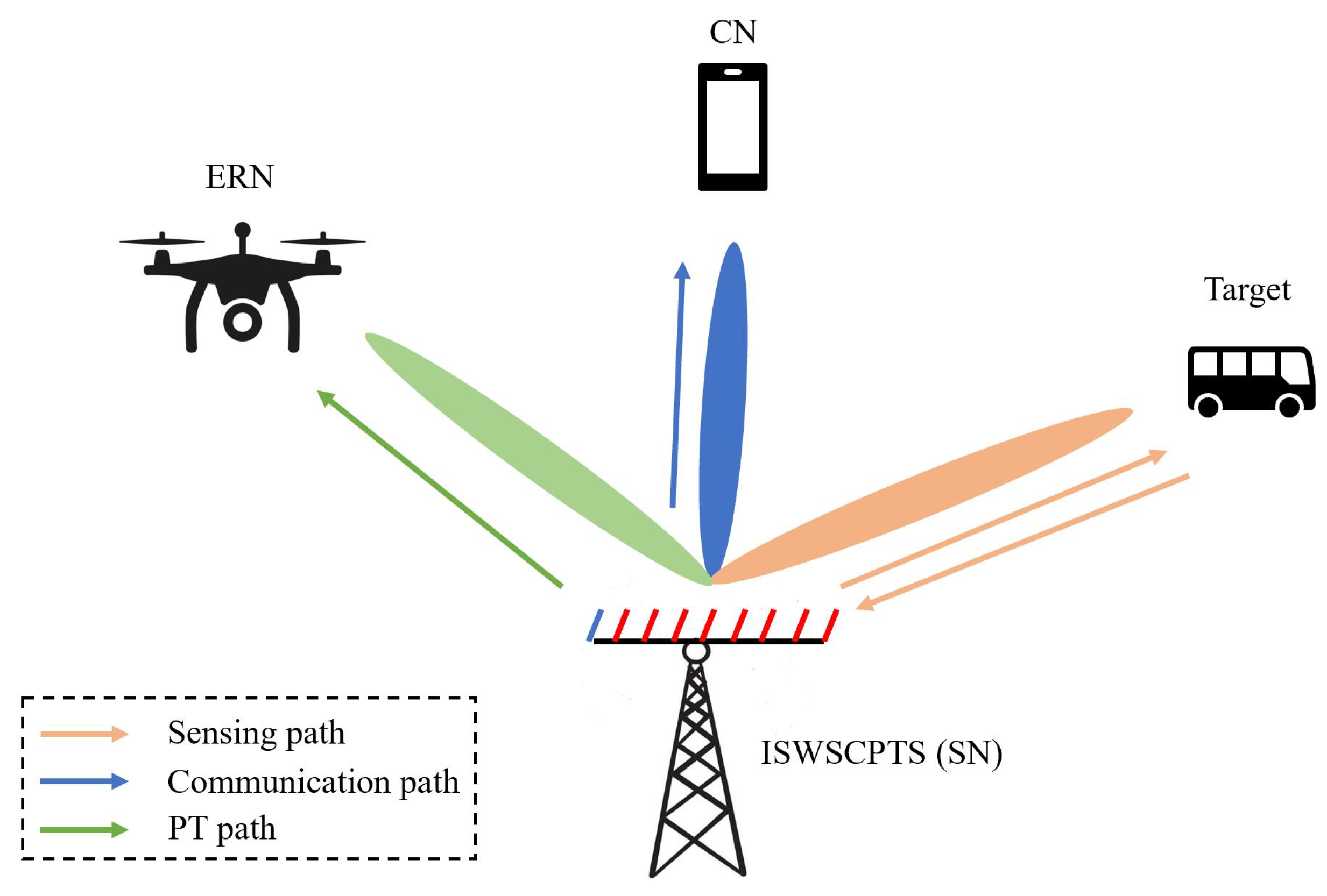
Figure 2.
The structure of CP-OTFS.
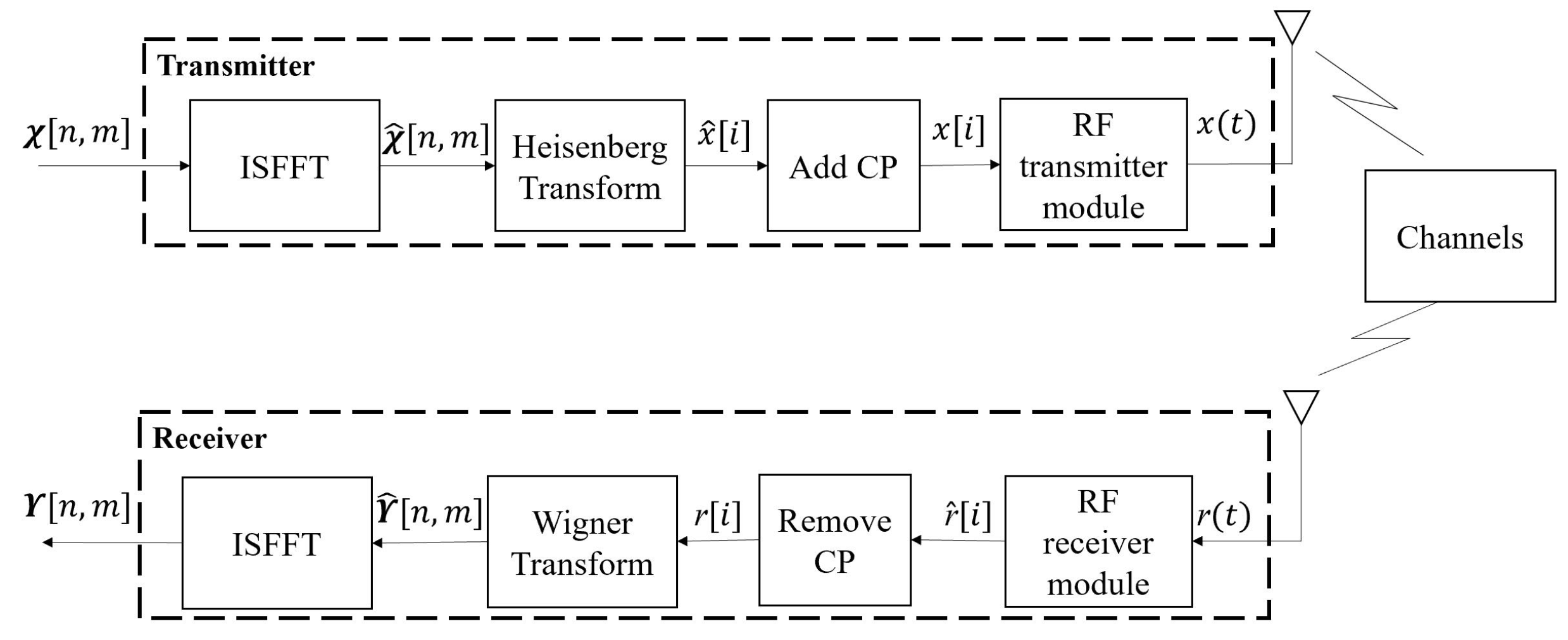
Figure 3.
The output of MF.
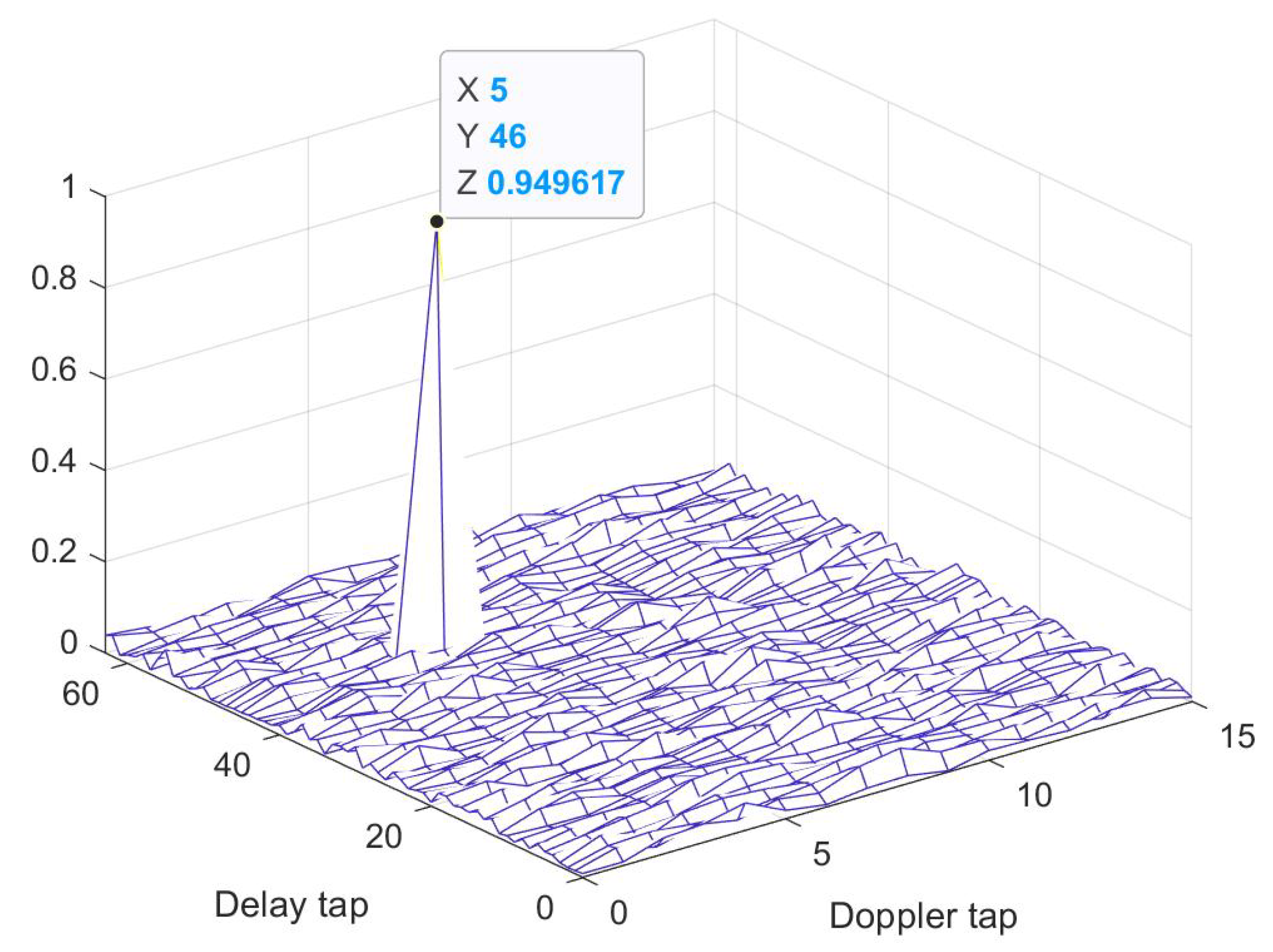
Figure 4.
Velocity RMSE vs relative velocity.
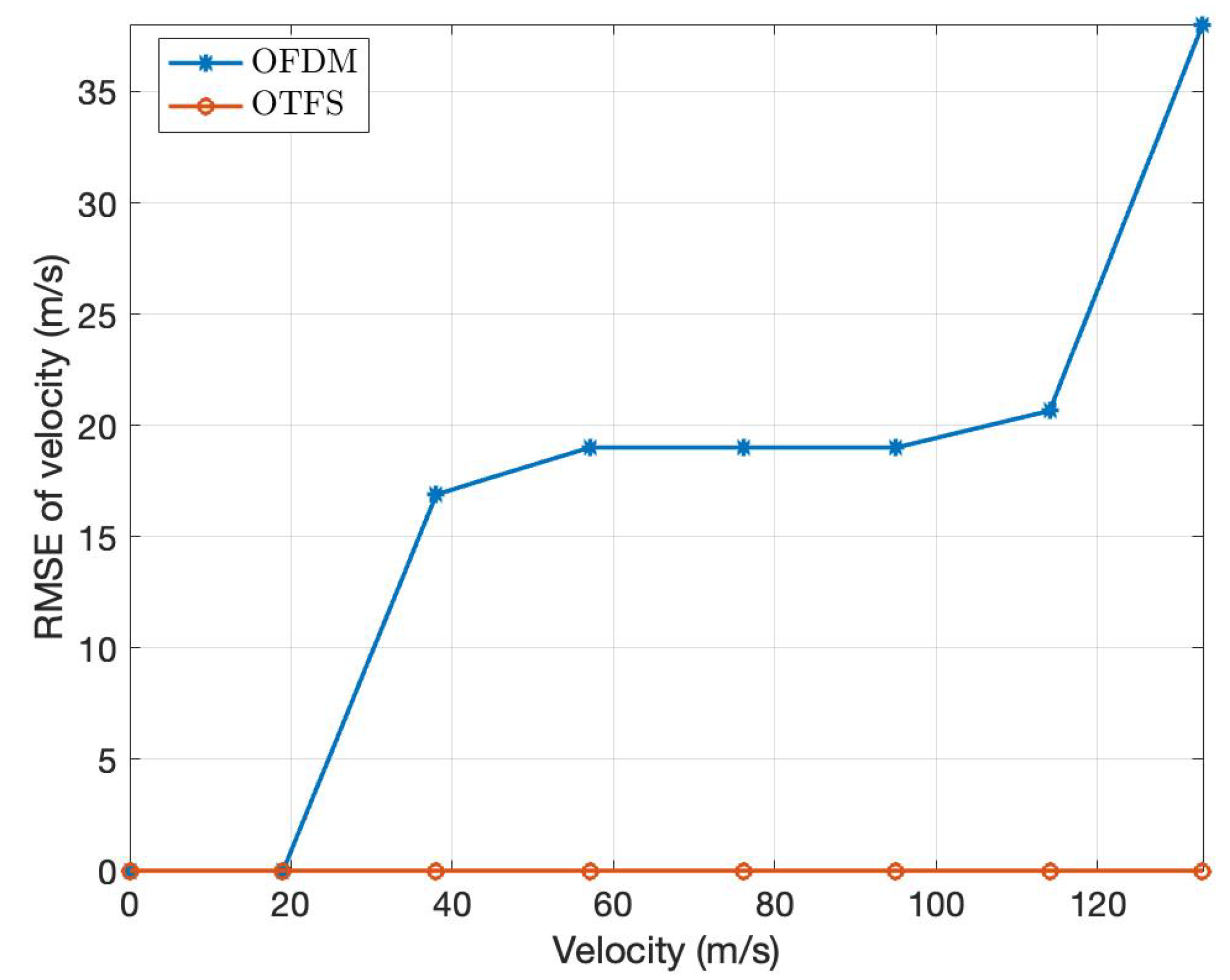
Figure 5.
TSC RMSE vs relative velocity.
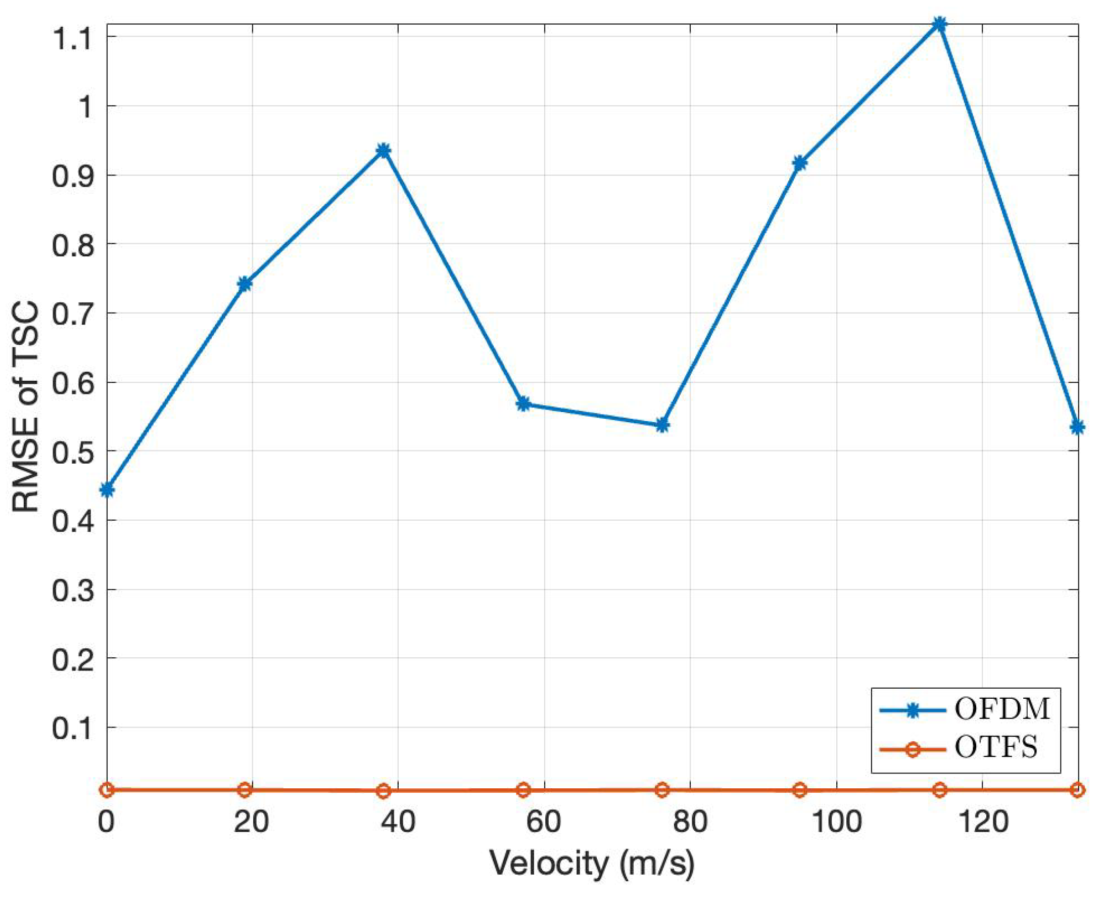
Figure 6.
AF of initial waveform.
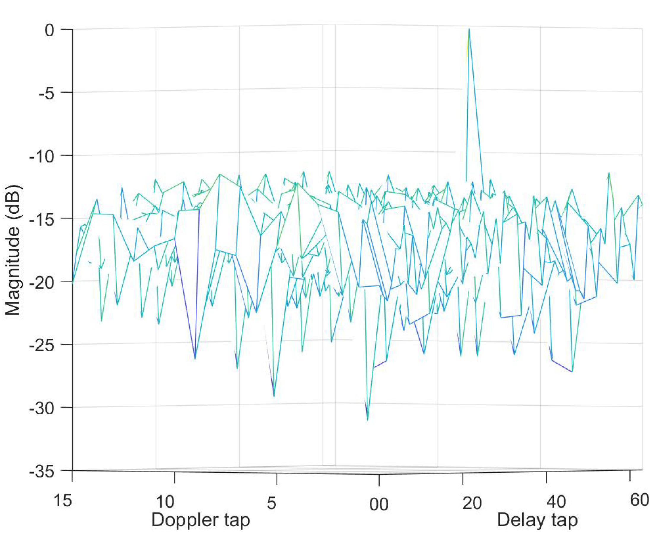
Figure 7.
AF of optimized waveform.
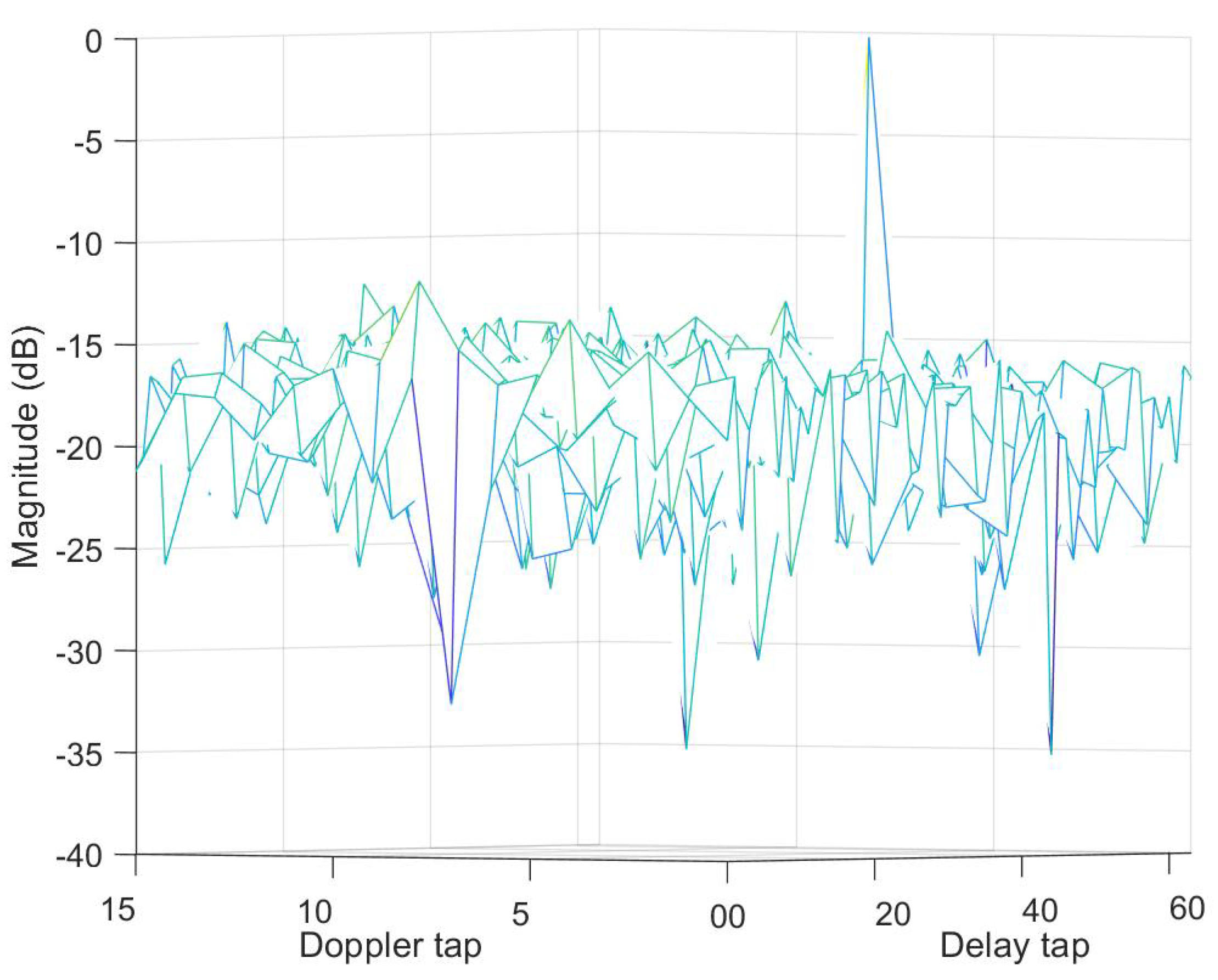
Figure 8.
ISL vs iterations.
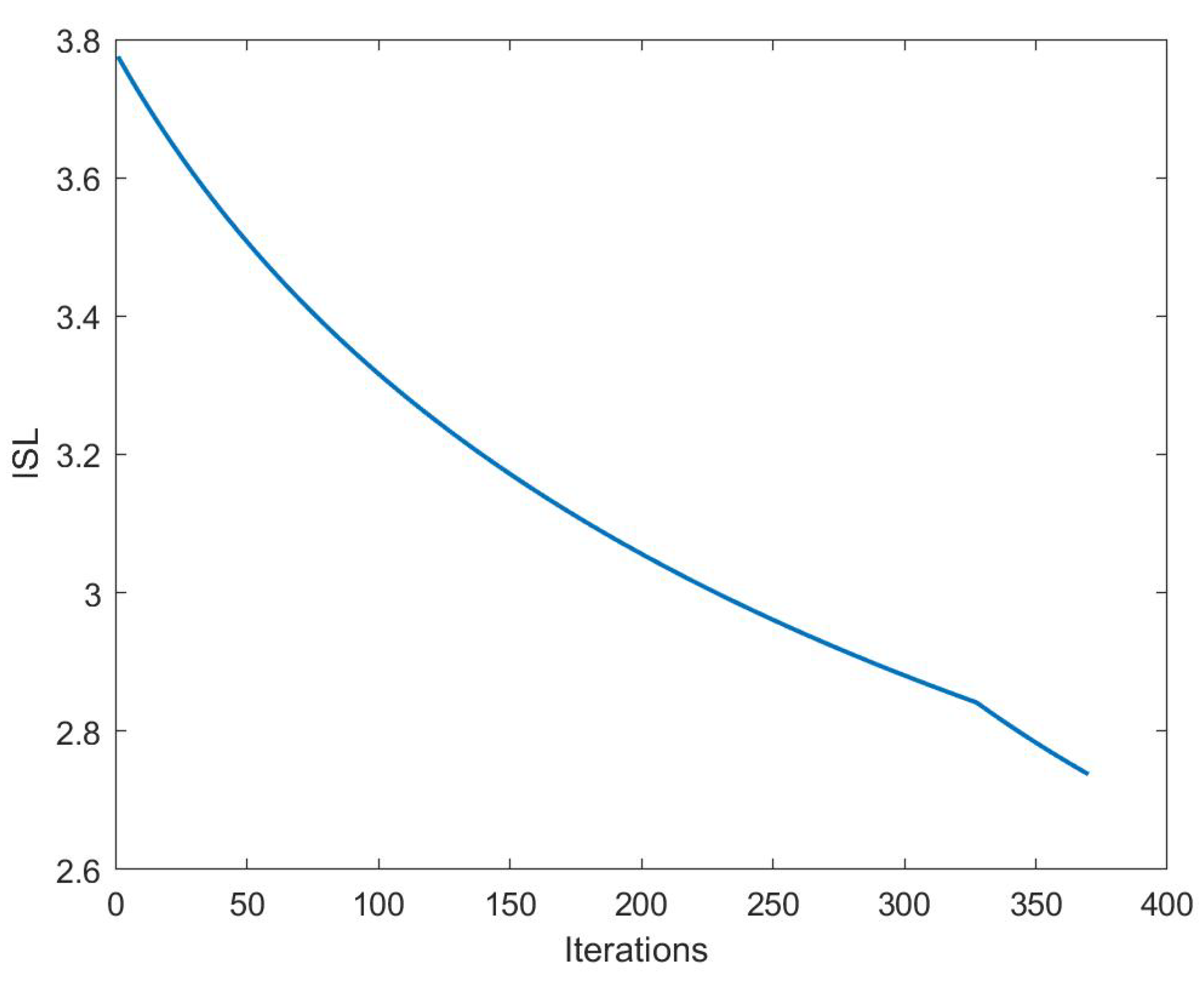
Figure 9.
TSC RMSE vs SNR under interference-free conditions.
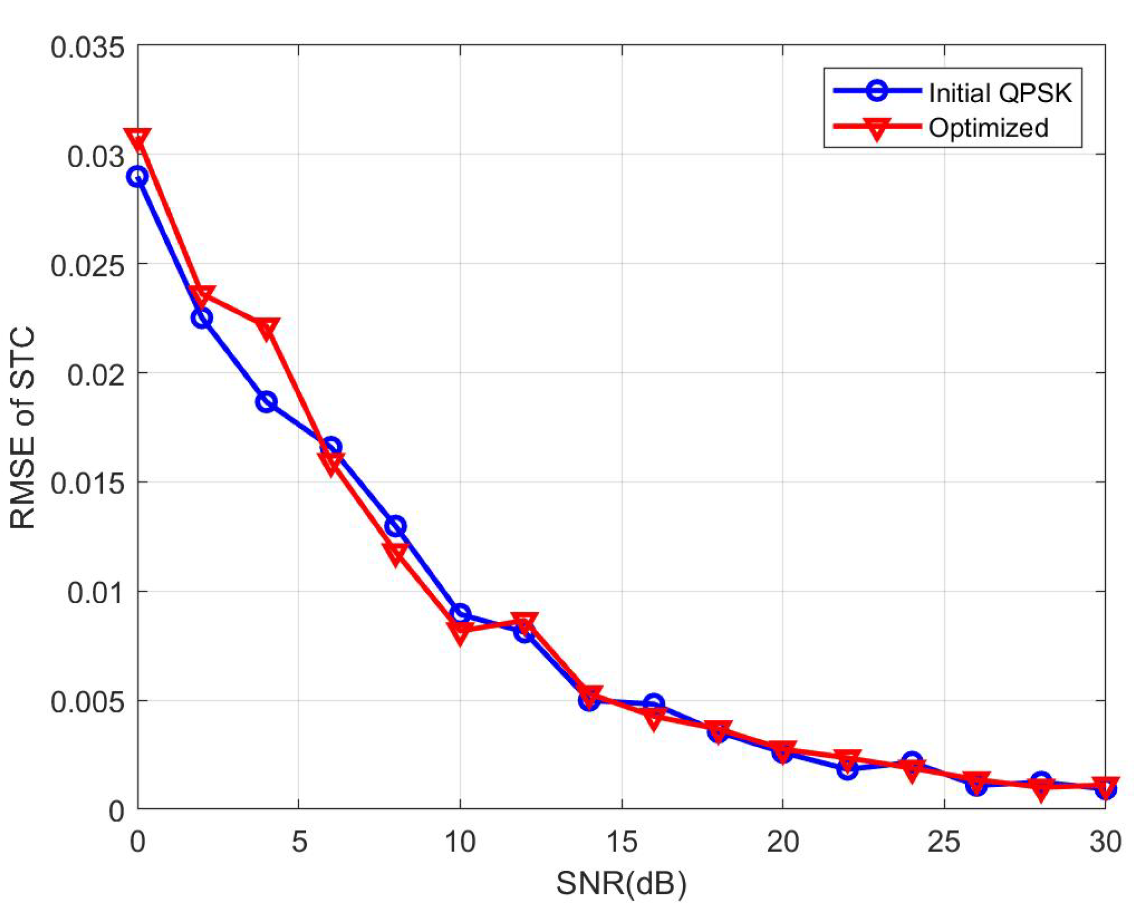
Figure 10.
TSC RMSE vs SNR under interference conditions.
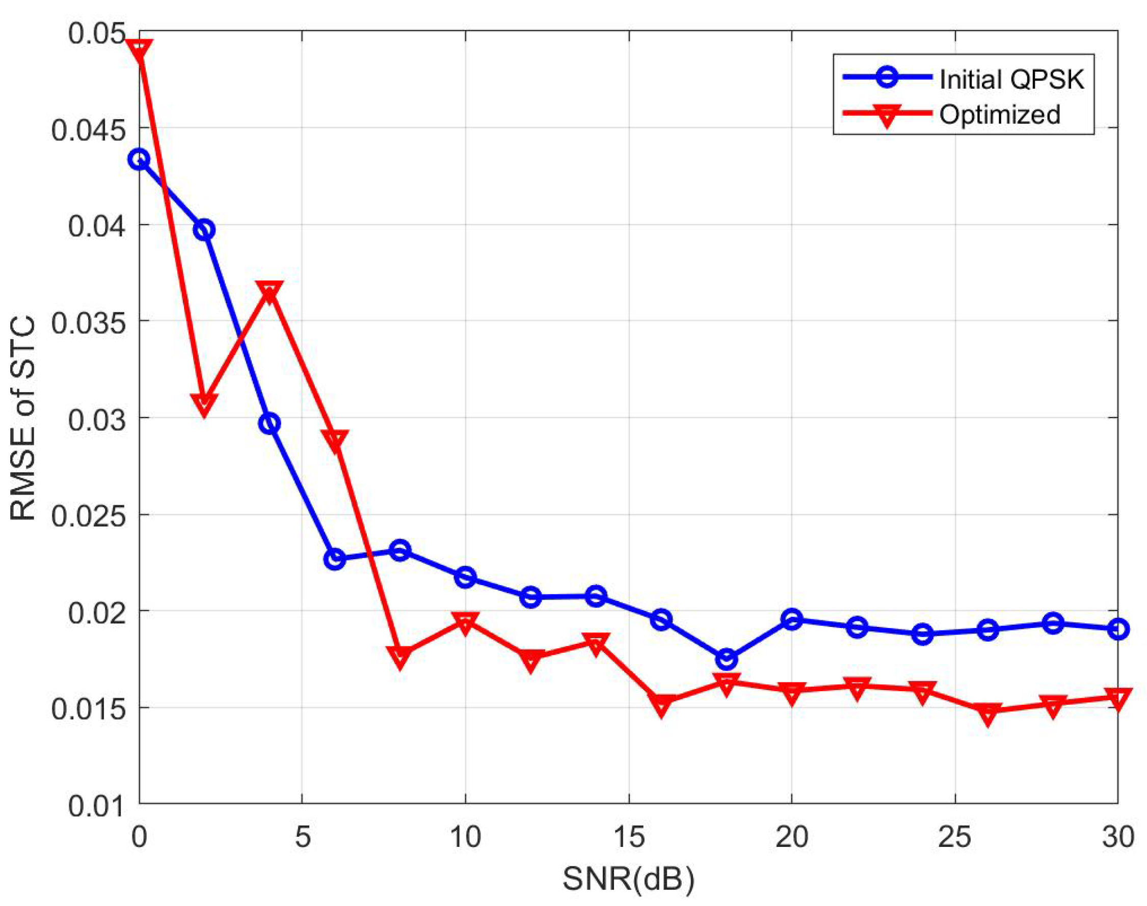
Figure 11.
Designed beamforming of different .
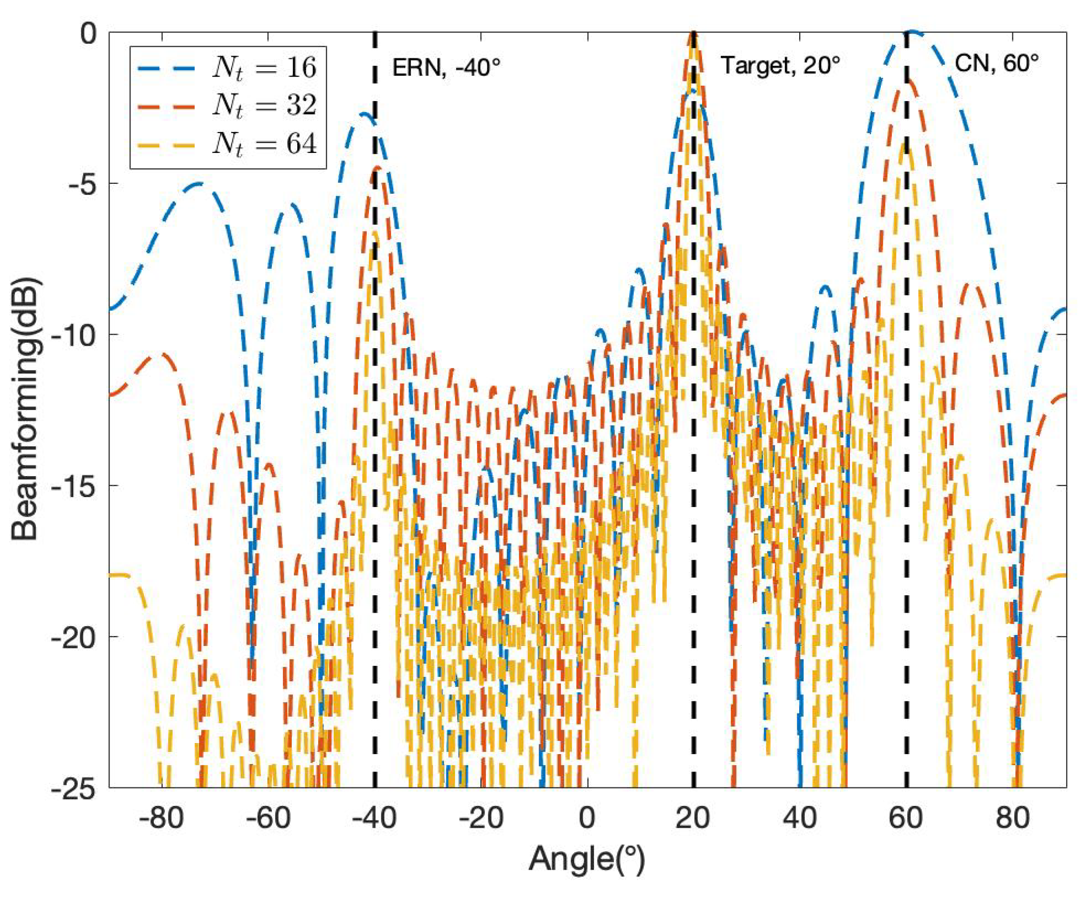
Figure 12.
Designed beamforming of different .
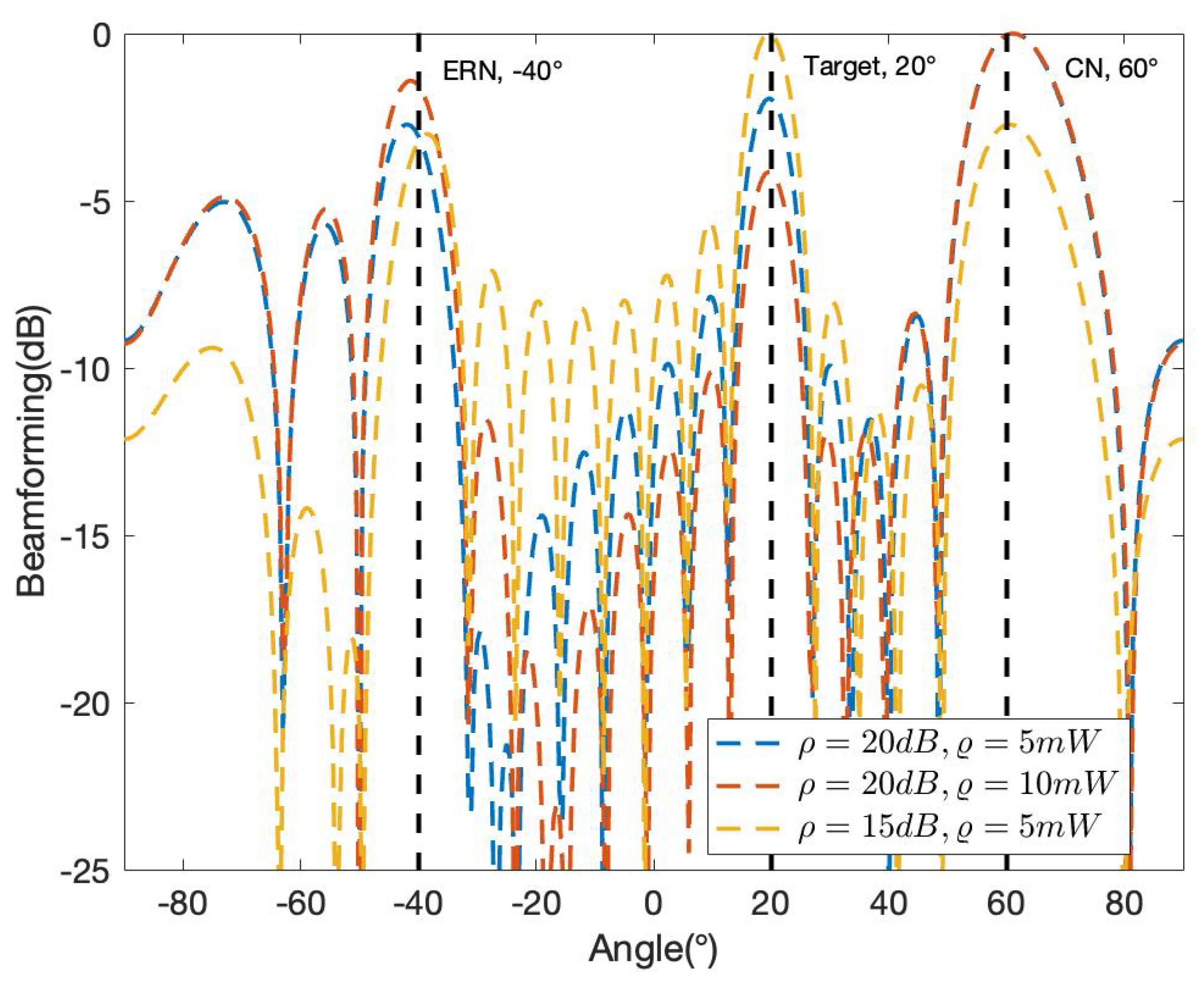

Table 1.
Basic simulation parameters.
| Symbol | Parameter | Value |
|---|---|---|
| Carrier frequency | 77 GHz | |
| N | Number of Doppler samples | 16 |
| N | Number of delay samples | 64 |
| B | Total bandwidth | 10 MHz |
| Subcarrier spacing | 156.250 kHz | |
| Range resolution | 14.99 m | |
| Velocity resolution | 19.01 m/s | |
| Unambiguous range | 959.336 m | |
| Unambiguous velocity | ±152.086 m/s |
Table 2.
Specific simulation parameters for SDR-BD.
| Symbol | Parameter | Value |
|---|---|---|
| Transmitting power | 1 W | |
| Variance of noise in CN | 0 dBm | |
| Variance of noise in SN | 10 dBm | |
| TSC | 0.8247+0.4709i | |
| Communication channel gain | 0.01 | |
| PT channel gain | 0.02 m | |
| Energy harvesting efficiency | 0.1 | |
| SNR required in CN | Configured | |
| Energy requirement in SN | Configured |
Disclaimer/Publisher’s Note: The statements, opinions and data contained in all publications are solely those of the individual author(s) and contributor(s) and not of MDPI and/or the editor(s). MDPI and/or the editor(s) disclaim responsibility for any injury to people or property resulting from any ideas, methods, instructions or products referred to in the content. |
© 2024 by the authors. Licensee MDPI, Basel, Switzerland. This article is an open access article distributed under the terms and conditions of the Creative Commons Attribution (CC BY) license (http://creativecommons.org/licenses/by/4.0/).
Copyright: This open access article is published under a Creative Commons CC BY 4.0 license, which permit the free download, distribution, and reuse, provided that the author and preprint are cited in any reuse.


