Clustering Coefficient of Lexicographic Products

Preprint

Article

Clustering Coefficient of Lexicographic Products

Altmetrics

Downloads

Views

Comments

Melissa Holly^*

This version is not peer-reviewed

This preprints belongs to the Topic

AI and Computational Methods for Modelling, Simulations and Optimizing of Advanced Systems: Innovations in Complexity

Submitted:

10 May 2024

Posted:

10 May 2024

You are already at the latest version

Alerts

Abstract

Clustering coefficient measures are key complex network analysis tools. We examine local and global clustering coefficient measures with respect to the lexicographic graph product. As a preliminary condition, we analyze the $K_3$ subgraph structure focused on vertex inclusion with respect to the product graph. From this structure, we determine both the clustering coefficient for the product graph vertices and the average clustering coefficient for the product graph.

Keywords:

Subject: Computer Science and Mathematics - Discrete Mathematics and Combinatorics

MSC: primary 05C82; secondary 05C75

1. Introduction

Clustering coefficient is a widely used tool in complex network analysis, particularly in social and neural networks. Introduced by Holland and Leinhardt (1971) [7], it is Strogatz and Watts (1998) who are credited with popularizing the average clustering coefficient of a graph as the small world property of a network [14]. Network analysis is a key area of study in applied graph theory that includes lexicographic networks (an example paper is [11].)

As mentioned, the various clustering coefficients are utilized in aspects of network structure analysis, especially with respect to community structure and information flow. A network vertex group with high local clustering coefficients indicates an area of high connectivity thus wide information exchange, while low clustering reflects structural holes. In information networks, the holes can indicate the presence of “gatekeepers" who control the information flow. Mark Newman’s Networks,Newman covers the various clustering coefficient measures in some detail. Although the number of triangles in a graph can be determined in polynomial time, this calculation relays little information about the relationship of the clustering in the lexicographic product as it relates to factor graph structure. In this note, we take a mathematical approach to the clustering coefficient so analysis of network structure is beyond the scope of this note. However, the information given here aids in network model construction and clustering investigation.

In this paper, the clustering coefficient calculations, and surrounding discussion, convey how the resulting community structure in the product graph is formed from the factor graph clustering. Theorem 1 gives the number of triangles in which a lexicographic product graph vertex can be found provided that the factor graphs are finite and simple. Theorem 2 provides the clustering coefficient of a lexicographic product graph vertex, while Corollary 3 presents the average clustering coefficient for this product graph.

As far as we know, there are only two other papers, [3,4], addressing clustering coefficient measures with respect to product graphs; and neither paper considers the lexicographic product. Calculating the clustering coefficient of any vertex, and the average clustering coefficient of the graph containing that vertex, provides little information regarding vertex

K_{3}

subgraph inclusion structure for the chosen graph. Several papers have been written regarding the minimum cycle basis structure of the lexicographic product graph ([1,8,9,10] as stated in [9]); but none of these papers address vertex

K_{3}

subgraph inclusion that is given in this note.

In Section 2 we provide notation and background information regarding the lexicographic graph product and regarding clustering coefficient measures. Section 3 contains the equation for the number of

K_{3}

subgraphs in which a product graph vertex can be found. The determination of the clustering coefficient for vertices, and the more global average clustering coefficient, are found in Section 4.

2. Background

Define a finite graph G by its vertex set

V (G)

and its edge set

E (G)

; and let

| V (G) |

and

| E (G) |

denote the number of elements in these two sets respectively. We assume general graph knowledge as found in [2]. Here, all graphs are finite and simple, thus disallowing both multiedges or loops. We give all graphs the same vertex labeling of

{0, 1, \dots, n - 1}

where graph order is

n = | V (G) |

. Graph size is denoted with

m = | E (G) |

. When reference is given concerning a specific graph G, then order and size are given by

n_{G}

and

m_{G}

, respectively. The open neighborhood of vertex x is

N (x)

while the closed neighborhood is

N [x]

. For graph order n, path graphs are

P_{n}

, complete graphs are

K_{n}

and empty graphs with n isolated vertices are denoted by

D_{n}

2.1. Lexicographic Graph Product

Graph product operations act on two graphs G and H referred to as the factor graphs. In graph theory, a homomorphism

ϕ : G \to H

is a vertex set mapping such that

{ϕ (x), ϕ (y)} \in E (H)

implies that edge

{x, y}

is in

E (G)

where

x, y \in V (G)

; thus preserving adjacency. A weak homomorphism is vertex map

ψ : G \to H

where an edge

{x, y}

in G implies either

{ψ (x), ψ (y)} \in E (H)

ψ (x) = ψ (y)

in H. For additional general information regarding graph products see [5].

The lexicographic graph product has vertex set of ordered pairs

(g, h)

produced by the Cartesian product

V (G) \times V (H)

, where

g \in V (G), h \in V (H)

. Pair

{(g, h), (g^{'} h^{'})}

is an edge in

G \circ H

if either

{g, g^{'}} \in E (G)

g = g^{'}

and

{h, h^{'}} \in E (H)

. Note that the operator

g = g^{'}

and

{h, h^{'}} \in E (H)

is a weak homomorphism.

K_{1}

is the unit for this product.

We sometimes indicate vertices in

G \circ H

g h

instead of

(g, h)

as shown in Figure 1 displaying

P_{2} \circ P_{3}

and

P_{3} \circ P_{2}

. In this figure, operator

{g, g^{'}} \in E (G)

is in dashed edges and operator

g = g^{'}

and

{h, h^{'}} \in E (H)

is in solid. As with other product graphs,

G \circ H

has projections from the product graph to its factors (see [5] for more information.) This results in the existence of “copies" of the two factors in the product graph. In Figure 1, note that the solid edges in the product are copies of H referred to as H layers; and some of the dashed lines are copies of G, analogously called G layers.

We refer to the edges generated by operator

{g, g^{'}} \in E (G)

as “spider edges". Notice that the spider edges join two adjacent H layers. Based on the definition for this product,

G \circ H

has order of

n_{G} \cdot n_{H}

and size

n_{G} (m_{H}) + m_{G} (n_{H}^{2})

. When referencing a vertex in G, we use

g_{G}

; and similarly, a vertex in H is

h_{H}

unless otherwise noted. The degree of a vertex in one of the factors is indicated by

deg (g_{G})

(or

deg (h_{H})

) where

g_{G}

(or

h_{H}

) is the specifric vertex in G (or in H).

For a specific vertex

x : = (g, h)

, denote the H layers that contain x as

H^{x}

, and let

H^{'}

indicate the H layers that do not contain x but do contain the vertices in

N (x)

The lexicographic product is associative but, with a few exceptions, it is not commutative. Displaying both

P_{2} \circ P_{3}

and

P_{3} \circ P_{2}

, Figure 1 shows this product aspect. Although the graph order for both of these product graphs is the same,

P_{2} \circ P_{3}

has 13 edges while the size of

P_{3} \circ P_{2}

is 11.

When G is connected, then

G \circ H

is connected. But when G is disconnected the product is disconnected with the number of connected components dependent on the number of components in G and in H.

2.2. Clustering Coefficient and Average Clustering Coefficient

The phrase “clustering coefficient" needs clarification as its usage varies in the literature. In this note, clustering coefficient refers specifically to the commonly utilized ratio focused on each vertex as calculated in Sage. To emphasize a vertex focus, we sometimes refer to the clustering coefficient as the vertex clustering coefficient. Given a specific vertex x, the clustering coefficient of x is:

\begin{matrix} c c (x) = \frac{total number of triangles that include x}{maximum number of triangles that could include x} \end{matrix}

(1)

The average clustering coefficient of a graph G,

a c c (G)

, is a global measure for G that can be compared to the density of

K_{3}

subgraphs in G. Utilizing the vertex clustering coefficient

c c (x)

over all

x \in V (G)

, average clustering coefficient is:

\begin{matrix} a c c (G) = \frac{\sum_{i = 1}^{n} c c (x_{i})}{n} \end{matrix}

(2)

Based on vertex degree, the denominator of

c c (x)

(\binom{deg (x)}{2})

. As a ratio, clustering coefficient has a maximum of 1 and a minimum of 0. Bipartite graphs have

a c c (G) = 0

as they are triangle free; while

K_{n}

with

n > 2

have

c c (x) = a c c (G) = 1

. Since

K_{1}

is the unit for the lexicographic product,

a c c (K_{1} \circ G) = a c c (G \circ K_{1}) = a c c (G)

. In this note, we interchange the use of “

K_{3}

subgraph" with “triangle". For additional information regarding clustering coefficient measures, see Newman [12].

3. Preliminaries

This section covers two topics: vertex degree and

K_{3}

subgraph inclusion structure of the product graph vertices. Both of these topics are essential to the next section that discusses the two product graph clustering coefficient measures.

3.1. Vertex Degree

The denominator of

c c ((g, h))

depends on the degree of a particular

(g, h)

G \circ H

where

deg (g, h) = deg (h_{H}) + deg (g_{G}) (n_{H})

for any

(g, h)

3.2. Vertex Inclusion in Triangle Subgraph Structure

This note has much focus on determining the triangle inclusion structure with respect to any vertex in a lexicographic product graph. Let

k_{3} (x)

be the

K_{3}

inclusion number of a vertex

x \in V (G)

where

k_{3} (x)

is defined as the total number of

K_{3}

subgraphs in G that include x.

Let

n_{1}

and

n_{2}

be two graph orders that may, or may not, be equal. Given two complete graphs

K_{n}

, we know that

K_{n_{1}} \circ K_{n_{2}}

produces the complete graph

K_{n_{1} n_{2}}

where the triangle structure is already known. As empty graph

D_{n}

has no edges, then it follows that

D_{n_{1}} \circ D_{n_{2}}

also has no

K_{3}

subgraphs.

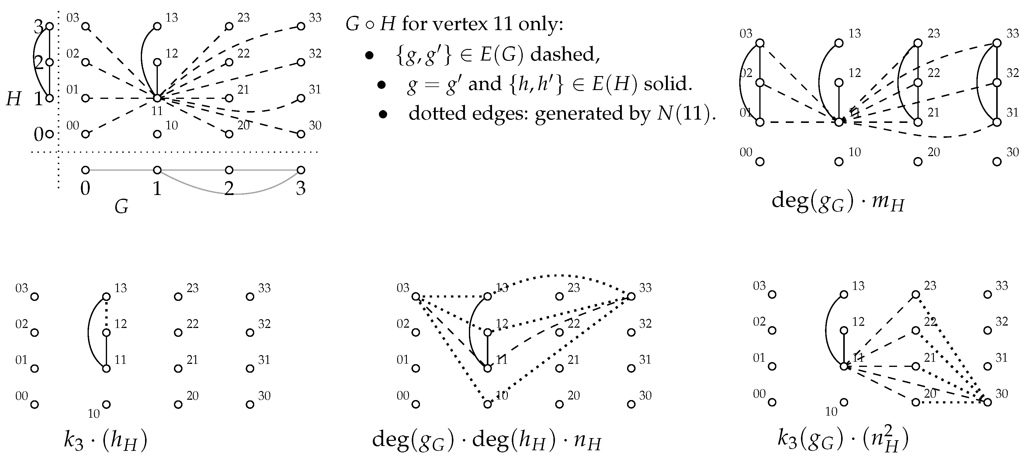
Figure 2 displays, on the left, the incident edges for only vertex 11 in

G \circ H

where G is in gray and disconnected H is in solid. As shown in this figure, the concept of the four

K_{3}

subgraph partitions is utilized in the proof of Theorem 1. Dotted edges represent spider edges in

N (11)

while dashed edges are spider edges for vertex 11.

In Figure 2, there are four edge partitions. The partition in the upper right reflects

K_{3}

subgraphs formed from a single

H^{'}

edge and two of 11’s spider edges. The lower left partition shows the triangle in

H^{11}

formed from two

H^{11}

edges and one

H^{11}

edge from

N (11)

. This

K_{3}

is not included in any of the other partitions. The bottom middle partition shows

K_{3}

subgraphs formed from one

H^{11}

edge, one 11 spider edge and one spider edge from

N (11)

. For greater clarity, this partition only displays two vertices in

N (11)

. Notice that as H is disconnected, spider edges from vertices 03 and 33 map to 10; but an edge from 11 to 10 does not exist so there is no triangle here. Lastly, the bottom right partition displays triangles that contain a single 11 spider edge and two spider edges for

20 \in N (11)

. As mentioned in the previous paragraph, the proof of Theorem 1 refers to this figure; thus providing additional explanation.

Theorem 1.

Let G and H be connected simple graphs. Then the number of

K_{3}

subgraphs in

G \circ H

that include specific vertex

(g, h)

is:

\begin{matrix} k_{3} (g, h) = deg (g_{G}) (m_{H} + deg (h_{H}) \cdot n_{H}) + k_{3} (h_{H}) + k_{3} (g_{G}) \cdot (n_{H}^{2}) \end{matrix}

(3)

Proof.

Suppose

G \circ H

has finite and simple factor graphs G and H. Let

(g, h)

be any vertex in

G \circ H

. There exist three types of edges with respect to

(g, h)

: the set of H layer edges (

H^{'}

edges plus

H^{(g, h)}

edges incident to

(g, h)

), the set of spider edges incident to

(g, h)

and the spider edges of vertices in

N ((g, h))

that are not incident to

(g, h)

but are incident to other members of

N ((g, h))

. After addressing disconnected factor graphs, we divide this proof into sections based on

K_{3}

subgraph partitions determined by the three edge types as shown in Figure 2.

Given a disconnected

G \circ H

k_{3} ((g, h))

is exclusive to any particular

(g, h)

, whether

G \circ H

is connected or not. In other words,

k_{3} ((g, h))

is relative to each vertex in each connected component. If H is disconnected, then the number of possible triangles in which

(g, h)

is located is reduced by the absence of an edge, or edges, in each H layer. This is similar for a disconnected G that generates a disconnected

G \circ H

(1) One

H^{'}

edge, and two

(g, h)

spider edges:

As operator

{g, g^{'}} \in E (G)

generates edges between adjacent H layers for any

(g, h)

, follow a spider edge s of

(g, h)

to a neighbor incident to an edge e in

H^{'}

. Then there exists another neighbor of

(g, h)

incident to e that is incident to another spider edge

s^{'}

(g, h)

. Denote this path by these edges. There are

deg (g_{G})

number of

(g, h)

’s neighbors; and for these neighbors, one can find

deg (g_{G}) \cdot m_{H}

number of distinct

(s, e, s^{'})

paths in this partition. This gives

deg (g_{G}) \cdot m_{H}

of this triangle type that contain

(g, h)

(2) Two

H^{(g, h)}

edges and one

H^{(g, h)}

edge from

N ((g, h))

For

(g, h)

in the product graph, let

h_{H}

be the vertex in H that is in

(g, h)

; and suppose that

h_{H}

shares a triangle in H with vertices y and z. Then

(g, h)

shares a triangle in

G \circ H

with

(g, y)

and

(g, z)

. In other words,

(g, h), (g, y)

and

(g, z)

are all in the same

H^{(g, h)}

layer; and they are contained in a

K_{3}

subgraph in that layer. The vertex set

{(g, h), (g, y), (g, z)}

triangle consists of two

H^{(g, h)}

edges incident to

(g, h)

and the

H^{(g, h)}

edge

{(g, y), (g, z)}

. Thus this triangle is not counted by the first set of partitions. This holds for any number of triangles in H that contain

h_{H}

, and

k_{3} (h_{H})

counts all of them by its definition.

(3) One

H^{(g, h)}

edge, one

(g, h)

spider edge, one

N ((g, h))

spider edge:

For

(g, h)

, let y be a neighbor of

(g, h)

H^{(g, h)}

. For all vertices z in

N ((g, h))

that are also adjacent to y due to operator

{g, g^{'}} \in E (G)

, there exist

((g, h), y, z, (g, h))

paths. As these paths involve one

H^{(g, h)}

edge, then the number of these paths for each such neighbor depends on

deg (h_{H})

and on

n_{H}

. The total number of these triangles is determined by

deg (g_{G})

resulting in

deg (g_{G}) \cdot deg (h_{H}) \cdot n_{H}

of these

K_{3}

subgraphs that distinctly include

(g, h)

(4) Two

(g, h)

spider edges and one

N ((g, h))

spider edge:

Now let

g_{G}, y

and z be vertices in G where set

{g_{G}, y, z}

forms a triangle in G and

g_{G}

is in

(g, h)

. Then there exists a

K_{3}

subgraph in

G \circ H

that contains vertices

(g, h), (y, h)

and

(z, h)

. Thus, vertex

(g, h)

has spider edges to not only

(y, h)

and

(z, h)

but also to all vertices in layers

H^{y}

and

H^{z}

. For any

(g, h)

spider edge to a neighbor in

H^{y}

, that neighbor has a spider edge to a vertex in

H^{z}

that is adjacent to

(g, h)

. Hence, a path exists for each vertex in

H^{z}

. Each path traces a

K_{3}

subgraph formed from two

(g, h)

spider edges plus one

(z, h^{z})

spider edge to

(y, h^{y})

so all H layer edges are excluded. There are

n_{H}

number of

(z, h^{z})

vertices, each of which has

n_{H}

number of spider edges to the vertices in

H^{y}

, and each is distinct from the others and distinct from the

(g, h)

(z, h^{z})

spider edge. As all previous counts contained at least one H layer edge, these

n_{H}^{2}

number of triangles are not previously counted by the other terms in equation 3. For a specific vertex

g_{G}

in G, if

g_{G}

is in more than one triangle in G, then

k_{3} (g_{G}) \cdot (n_{H}^{2})

in equation (3) counts the additional triangles in the product graph.

Concerning any vertex

(g, h) \in V (G \circ H)

, there are

deg (g_{G}) \cdot m_{H}

number of

H^{'}

edges in triangles with

(g, h)

that are counted in partition (1). Vertex

(g, h)

has

deg (g, h) = deg (h_{H}) + deg (g_{G}) (n_{H})

incident spider edges, all of which are counted in partitions (1), (3) and (4). There are

deg (g_{G}) \cdot deg (h_{H}) \cdot n_{H}

neighbors of

(g, h)

, all of whose spider edges to other vertices in

N ((g, h))

are counted. The number of factor graph triangles that include

g_{G}

and

h_{H}

are counted. If an edge e has been missed, then e must be in a G layer but not in a triangle in that layer, all of which are counted by equation (3). Therefore,

k_{3} (g, h) = deg (g_{G}) (m_{H} + deg (h_{H}) \cdot n_{H}) + k_{3} (h_{H}) + k_{3} (g_{G}) \cdot (n_{H}^{2})

. □

4. Clustering Coefficient for Lexicographic Product

We now address the clustering measures for

G \circ H

. Equation (4) gives the clustering coefficient for

(g, h)

while equation (5) presents the

a c c (G \circ H)

utilizing vertex partitions.

Consider

K_{1}

that has average clustering coefficient of zero. As

K_{1}

is the unit for the lexicographic product, then for any

K_{n}

, product

K_{1} \circ K_{n}

(or

K_{n} \circ K_{1}

due to commutativity of

K_{n_{1}} \circ K_{n_{2}}

) results in

K_{n}

. This produces the vertex clustering coefficient and average clustering coefficient of

K_{n}

. When

n = 2

K_{2} = P_{2}

which has

a c c (P_{2}) = 0

. Thus

a c c (K_{1} \circ K_{2}) = a c c (K_{2}) = 0

For

n_{1}, n_{2} \geq 3

, allowing both equality and inequality of

n_{1}

and

n_{2}

, it is a fact that all

K_{n_{1}} \circ K_{n_{2}}

result in

K_{n_{1} n_{2}}

. Thus

a c c (K_{n_{1}} \circ K_{n_{2}}) = a c c (K_{n_{1} n_{2}}) = 1

when

n_{1}, n_{2} \geq 3

. However, take note that

K_{2} \circ K_{2}

produces

K_{4}

. Although

a c c (K_{2}) = 0

, this product results in

K_{4}

with

a c c (K_{4}) = 1

. In fact, for any

K_{2} \circ K_{n} ≅ K_{n} \circ K_{2}

where

n \geq 2

, even though

a c c (K_{2}) = 0

a c c (K_{2} \circ K_{n}) = 1

Now contemplate

D_{n_{1}}

, the graph of

n_{1}

isolated vertices, and its lexicographic product with

D_{n_{2}}

, where equality of the orders is permitted. As no edges exist, the definition of lexicographic product fails to generate edges in

D_{n_{1}} \circ D_{n_{2}}

. Hence,

a c c (D_{n_{1}} \circ D_{n_{2}}) = 0

. Also note that

K_{1} = D_{1}

The proof of the following theorem is found in the definition of clustering coefficient given by equation (1) and the proof of equation (3), plus the fact that the maximum

K_{3}

inclusion number is

(\binom{deg (g, h)}{2})

Theorem 2.

Suppose G and H are both simple graphs. Then the vertex clustering coefficient

c c (g, h)

of any vertex

(g, h)

G \circ H

is:

\begin{matrix} c c (g, h) = \frac{deg (g_{G}) (m_{H} + deg (h_{H}) \cdot n_{H}) + k_{3} (h_{H}) + k_{3} (g_{G}) \cdot (n_{H}^{2})}{(\binom{deg (g, h)}{2})} . \end{matrix}

(4)

▪

Based on the definition of the average clustering coefficient, we give Theorem 3 without proof.

Theorem 3.

For finite and simple graphs G and H, the average clustering coefficient of

G \circ H

with order

n_{G} n_{H}

over all vertices

(g, h)

is:

\begin{matrix} a c c (G \circ H) = \frac{\sum_{i = 1}^{n_{1} n_{2}} c c ({(g, h)}_{i})}{n_{G} n_{H}} . \end{matrix}

(5)

▪

References

F. Berger (2004) Minimum Cycle Bases of Graphs. Dissertation, Technische Universität München.
G. Chartrand, L. Lesniak, P. Zhang (2016) Graphs & Digraphs, 6th Ed.. DCRC Press, Boca Raton, FL.
R. J. M. Demalerio, R. G. Eballe (2022) Global clustering coefficient of the products of complete graphs. Asian Research Jrnl. of math. v.18(6). 62-69. [CrossRef]
R. J. M. Demalerio, R. G. Eballe (2022) Clustering coefficient of the tensor product of graphs. Asian Research Jrnl. of math. v.18(6). 36-42. [CrossRef]
R. Hammack, W. Imrich, S. Klavžar (2011) Handbook of Product Graphs, 2nd Ed.. CRC Press, Boca Raton, FL.
F. Harary (1959) On the group of the composition of two graphs. Duke Math. Jrnl. v.26(1) March. 29-34.
P.W. Holland, S. Leinhardt (1971) Transitivity in structural models of small groups. Comparative Group Studies v.2(2). p.107-124. [CrossRef]
M. Hellmuth, P.J. Ostermeier, P.F. Stadler (2012) Minimum cycle bases of lexicographic products. ARS Math. Contemporanea. https://amc-journal.eu. 223-234.
M. M. M. Jaradat (2008) Minimal cycle bases product of graphs. Discuss. Math., Graph Theory v.28. 229-247. [CrossRef]
A. Kaveh, R. Mirzaie (2008) Minimal cycle bases of graph products for the forced method of frame analysis. Commun. Numer. Methods Eng. v.24. 653-669. [CrossRef]
F. Li (2020) On forwarding indices of lexicographic product networks. Concurrency and computation 32(23). [CrossRef]
M. Newman (2018) Networks, 2nd Ed.. Oxford Univ. Press, Oxford, United Kingdom.
G. Sabidussi (1959) The composition of graphs. Duke Math. Jrnl. v.26(4) December. 693-696.
S. Strogatz, D.J. Watts (1998) Collective dynamics of ’small-world’ networks. Nature 393(6684). 440–442. [CrossRef]

Figure 1.

P_{2} \circ P_{3}

and

P_{3} \circ P_{2}

showing noncommutativity of lexicographic product.

Figure 1.

P_{2} \circ P_{3}

and

P_{3} \circ P_{2}

showing noncommutativity of lexicographic product.

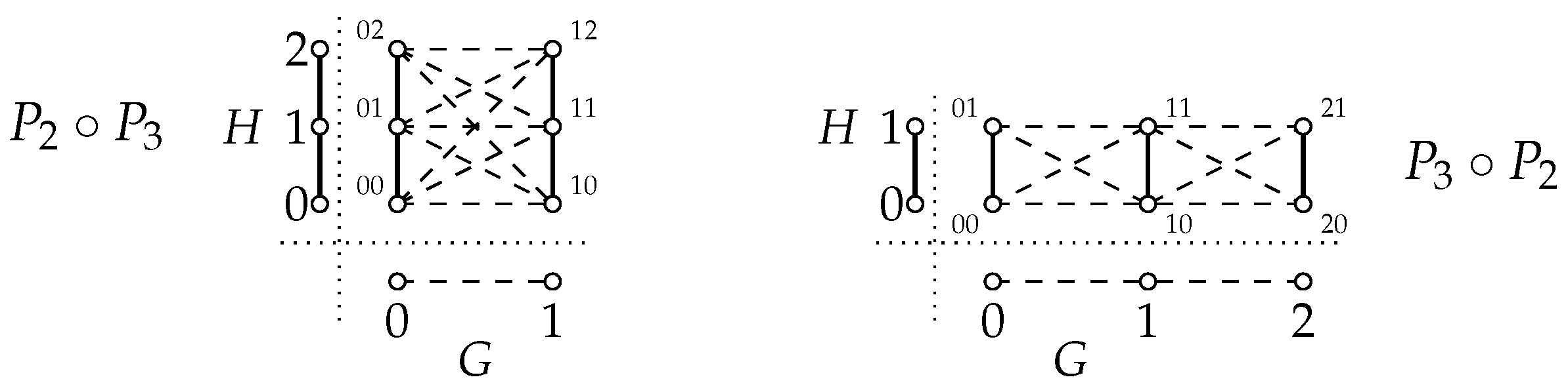
Figure 2.

G \circ H

with four

K_{3}

subgraph partition examples for only vertex 11.

Figure 2.

G \circ H

with four

K_{3}

subgraph partition examples for only vertex 11.

Disclaimer/Publisher’s Note: The statements, opinions and data contained in all publications are solely those of the individual author(s) and contributor(s) and not of MDPI and/or the editor(s). MDPI and/or the editor(s) disclaim responsibility for any injury to people or property resulting from any ideas, methods, instructions or products referred to in the content.

© 2024 by the authors. Licensee MDPI, Basel, Switzerland. This article is an open access article distributed under the terms and conditions of the Creative Commons Attribution (CC BY) license (http://creativecommons.org/licenses/by/4.0/).

Copyright: This open access article is published under a Creative Commons CC BY 4.0 license, which permit the free download, distribution, and reuse, provided that the author and preprint are cited in any reuse.

MDPI Initiatives

Important Links

Choose an area of interest and we will send you notifications of new preprints at your preferred frequency.

Disclaimer

Clustering Coefficient of Lexicographic Products

Abstract

1. Introduction

2. Background

2.1. Lexicographic Graph Product

2.2. Clustering Coefficient and Average Clustering Coefficient

3. Preliminaries

3.1. Vertex Degree

3.2. Vertex Inclusion in Triangle Subgraph Structure

4. Clustering Coefficient for Lexicographic Product

References

MDPI Initiatives

Important Links

Subscribe