Research on Financial Risk Management Early Warning Model for Chinese Enterprises

Preprint

Article

Research on Financial Risk Management Early Warning Model for Chinese Enterprises

Altmetrics

Downloads

102

Views

Comments

A peer-reviewed article of this preprint also exists.

This version is not peer-reviewed

Submitted:

07 May 2024

Posted:

08 May 2024

You are already at the latest version

Alerts

Abstract

This paper utilizes the 2020 financial data of A-share listed companies, both ST and non-ST, as the data sample. The model is constructed employing the Factor-Logistic fusion algorithm. Eight key indicator factors were selected from the frameworks of profitability, solvency, operating capacity, development potential, shareholder retained earnings, cash flow and asset growth. An independent indicator system was subsequently established to address the issue of collinearity among risk indicators. The results of model are presented in the form of probabilities, enhancing the interpretability of model. The weights of the features indicate the influence of different features on the final outcome. The model achieves a prediction accuracy of over 89%, with an AUC score exceeding 95%. Finally, by applying the principles of interval estimation theory in statistical hypothesis testing, the risk levels are categorized as A-level representing significant risk, B-level representing moderate risk, C-level representing minor risk and D-level representing no risk. This paper aims to provide a comprehensive definition of a universal financial risk management warning model for enterprises, applicable to all enterprises in China.

Keywords:

Subject: Business, Economics and Management - Finance

1. Introduction

Over the past four decades of reform and opening up in China, the GDP has increased from 367.8 billion yuan in 1978 to 126 trillion yuan in 2023 [1]. The total market capitalization of around 5,200 listed companies on China's three major exchanges also reached approximately 90 trillion yuan in 2023, indicating a rapid development of the stock market in recent decades. However, due to the relatively late start and rapid development of information technology, various regulatory measures implemented in China's securities market are still not perfect [2]. These include risks such as illegal operations, fraud, manipulation of profits, and poor management. Worse still, the global COVID-19 pandemic that began in 2020 has led to a decline in the world economy. Facing the threat of the global pandemic, competition in the big data market has become even more intense. Both domestic and foreign enterprises have increased their attention to stabilizing their financial conditions, placing greater emphasis on improving their financial situation and perfecting their financial risk management and early warning systems.

Therefore, it is particularly important for investors, governments, banks, creditors, managers, employees, and other stakeholders to establish a scientific, comprehensive, flexible, and accurate enterprise financial risk management and early warning model in China. Such a model can categorize and promptly warn of different levels of financial risk crisis in enterprises, reflecting and eliminating risks at their inception [3].

This paper relies on the financial data of ST and corresponding non-ST enterprises listed on China's A-share market in 2020 to develop a generic enterprise financial risk management and early warning model. The model utilizes the Factor-Logistic fusion algorithm for modeling, ultimately dividing enterprises into four different financial risk levels (A-level representing significant risk, B-level representing moderate risk, C-level representing minor risk, and D-level representing no risk).

The core innovations of this paper are as follows:

Selection of key financial indicators for the financial risk management and early warning model.
Utilization of the Factor-Logistic fusion algorithm to construct the financial risk management and early warning model.
Categorization of risk levels within the financial risk management and early warning model.

2. Related Literature

The concept of financial early warning dates back to 1932, when Fitz Partrick initiated research on single-variable bankruptcy prediction [4]. In 1966, Beaver further expanded on Fitz Partrick's approach by introducing cash flow indicators to establish a financial distress warning model [5]. Subsequently, Altman employed multivariate linear discrimination for financial risk warning in 1968, resulting in the development of the Z-Score model [6]. In 1980, Ohlson applied the multivariate Logistic regression model to financial early warning [7]. In 1993, Ofek's research found that the higher a company's financial leverage, the greater the likelihood of escaping financial distress [8]. Ana M. Aguilera and others combined principal component analysis with Logistic regression in 2006 to predict corporate default, though the practical significance of the principal components was difficult to interpret [9].

Moreover, machine learning techniques have been widely used in model development. Franco Varetto employed genetic algorithms to study corporate bankruptcy risk in 1998 [10]. Jae H. Min and Young-Chan Lee applied the support vector machine method to predict credit risk in listed companies in 2005 [11]. With the advancement of information technology, Odom and others used neural networks in 1990 to predict corporate bankruptcy [12,13].

In China, the earliest theoretical development was in 1996, when Zhou Shouhua and others borrowed from Altman's Z-Score model and added cash flow ratios [14]. Since then, various scholars have studied the impact of different financial indicators on the model.

3. Model Research

3.1. Sample Source

The sample data for this study was derived from the financial indicator data of 4,254 A-share listed companies in 2020, sourced from TongHuaShun Finance [15]. The sample design encompassed both a sample group and a matched group.

In selecting the sample group, companies that were specially treated (ST and *ST) due to "abnormal financial conditions" were chosen as the markers of financial distress (i.e., the research subjects). Statistics revealed that there were 200 A-share listed companies with ST and *ST status in 2020. After excluding companies with missing indicator data, 182 companies with valid data remained. Following the treatment of outlier values, 160 listed companies were selected as the sample group for our modeling, including 80 manufacturing enterprises and 80 non-manufacturing enterprises. Statistics further indicate that 80% of these 160 ST and *ST companies are privately owned, while 20% are state-owned enterprises.

For the selection of the matched group, 160 financially healthy companies were chosen based on the method of finding companies with the closest ending asset totals to those of the ST and *ST companies. The proportion of enterprise attributes in the matched group was kept identical to that of the sample group.

In total, the combined matched sample comprises financial data from 320 companies.

3.2. Indicator Selection

Currently, there is no unified standard for establishing an indicator system in research literature on financial early warning. Different scholars have chosen different indicators in their research processes. This paper employed the Delphi method to select key financial indicators from the set of financial indicator knowledge graphs as research variables [16]. These eight financial indicators, after repeated deliberation by experts, comprehensively cover the core indicators of a company's various aspects of operations, management, and finance, thus forming the financial feature dimensions of this study's financial risk early warning model.

In addition, enterprise nature (private or state-owned) and enterprise industry classification (manufacturing or non-manufacturing) were also included as non-financial feature dimensions of our risk early warning model. The purpose of incorporating these two indicators is to explore whether they have a positive enhancing effect on the model.

The selected indicators are presented in Table 1, and partial financial indicator data is shown in Table 2 (variable labels will be used in place of indicator names in the following text).

3.3. Indicator Selection

Table 3 presents the descriptive statistics of the data, from which it is evident that the maximum value of the solvency indicator is relatively large. In a multi-indicator evaluation system, different evaluation indicators often possess distinct measurement units and scales due to their varying natures. When there are significant differences in the levels of various indicators, analyzing them directly using their original values would highlight the influence of those with higher numerical values while relatively weakening the impact of those with lower numerical levels. Consequently, to ensure the reliability of the results, it is necessary to standardize the original indicator data.

The correlation coefficient is a metric used to measure the degree of correlation between observed data. Generally, a higher correlation coefficient indicates a stronger correlation.

As can be seen from Table 4, there is correlation between each pair of financial indicators, mostly at a low or moderate level. However, there is basically no correlation between non-financial indicators and other indicators on a pairwise basis.

The results of the significance analysis shown in Table 5 indicate that among the ten indicators, only profitability, leverage, turnover, and cash flow indicators exhibit significance at the 0.05 level. This means that, without data transformation, only these four indicators play a decisive role, while the remaining indicators contribute little to the model. There are two primary reasons for this outcome:

The indicators themselves may not be meaningful for the model. Through analysis, we found that non-financial indicators such as enterprise nature and industry classification do not contribute positively to the model. Even from the perspective of correlation, they are negatively correlated with other financial indicators. This suggests that, in terms of enterprise nature, there is no significant difference between state-owned enterprises and private enterprises in determining whether a listed company is ST or non-ST. As for industry classification, there is no need to distinguish between manufacturing and non-manufacturing industries when modeling. This indirectly supports the feasibility of using a general financial risk warning model for enterprise risk prediction.
There is a strong collinearity among financial indicators, and it is necessary to consider removing the multicollinearity between indicator variables. Removing financial indicators would lead to incomplete interpretability, so factor analysis can be used to avoid multicollinearity among financial indicators.

3.4. Factor Analysis

Based on the conclusions drawn from the previous analysis, this paper abandons the two non-financial indicators of enterprise nature and industry classification and constructs a model solely composed of continuous financial indicators. Factor analysis is an extension of principal component analysis (PCA), which is more inclined to describe the correlation between the original variables compared to PCA [17,18]. The factor analysis method in SPSS software is used for calculation.

First, a KMO measure and Bartlett's test are conducted on the eight financial indicators. The results are shown in Table 6:

From the results, we can see that the Bartlett statistic is 486.096, and its corresponding significance probability is 0.000, which is less than the significance level of 0.05. This indicates that the correlation matrix is not an identity matrix, therefore suitable for factor analysis. The KMO value is greater than 0.6, suggesting that the factor analysis results are satisfactory.

Next, using SPSS software, we automatically calculated the eigenvalues and contribution values of each principal component, as detailed in Table 7:

Taking into account the amount of information represented by the actual indicators and the comprehensiveness of the indicators, we still specify the retention of eight factors. It is believed that these eight common factors reflect the comprehensive information of the original variables. Therefore, factor analysis in this paper only serves the purpose of eliminating collinearity.

Additionally, as can be seen from the scree plot of eigenvalues (Figure 1), the eigenvalue for Factor 8 is not particularly small. Moreover, the differences between Factors 2 to 8 are similar, making it difficult to justify discarding any one of them. Therefore, it is concluded that retaining all eight factors will not result in any loss of information.

In order to clearly reflect the relationship between the principal component factors and the original variables, we have output the rotated factor loadings as shown in Table 8:

From Table 8, it can be observed that the asset growth indicator has a relatively large loading on Factor 1, hence it is named as Asset Growth Factor (F1). The solvency indicator has a significant loading on Factor 2, thus it is designated as Solvency Factor (F2). The profitability indicator exhibits a strong loading on Factor 3, leading to its denomination as Profitability Factor (F3). Similarly, the turnover indicator has a prominent loading on Factor 4, making it Turnover Factor (F4). The earnings indicator is heavily loaded on Factor 5, naming it Earnings Factor (F5). The cash flow indicator displays a significant loading on Factor 6, resulting in its designation as Cash Flow Factor (F6). The liquidity indicator has a strong loading on Factor 7, naming it Liquidity Factor (F7). Finally, the leverage indicator is loaded on Factor 8, naming it Leverage Factor (F8). The results of the factor analysis firmly validate the strategy of selecting these eight factors.

To establish an accurate relationship between the common factors and the indicators, it is necessary to express the common factors as linear combinations of the individual variables. Using the regression method within the factor analysis function of SPSS software, a factor score coefficient matrix can be generated, as shown in Table 9. This matrix allows us to calculate the factor scores based on the factor score coefficients and the standardized values of the original variables. With these factor scores, further analysis of the financial indicators can be conducted.

3.5. Logistic Regression

In this paper, ST listed companies are coded as 0, and non-ST listed companies are coded as 1, serving as the dependent variable. Using the eight influencing factors identified through factor analysis as independent variables, a Logistic regression analysis is conducted with the assistance of SPSS software. The regression results are presented in Table 10:

Based on the analysis above, it is evident that each influencing factor in the model is crucial, contributing approximately the same variance. Under such data validation, removing or replacing any factor would result in significant information loss for the model. Therefore, this article opts to establish the model at a significance level of 0.1, retaining all eight influencing factors intact.

When using a cut-off threshold of 0.5, the observation of the model's performance on the sample data is presented in Table 11:

Table 11 indicates that the Logistic regression model achieves an overall prediction accuracy of 89.7% for the sample data. The model incorporates a comprehensive set of dimensional features and exhibits strong explanatory power, suggesting that its predictive capability is reliable and well-supported.

3.6. Risk Level Classification

Based on the Delphi method, this article divides enterprise financial risks into four categories: A-level representing significant risk, B-level representing moderate risk, C-level representing minor risk, and D-level representing no risk. This classification is considered more practical and widely accepted by relevant personnel in enterprises and institutions based on years of industry experience and qualitative analysis.

To classify financial risks based on these four levels, this article proposes an innovative approach. Drawing on the significance testing perspective proposed by Fisher in statistics, we set 90% (general significance level) and 95% (high significance level) as confidence thresholds. We believe that the accuracy of classifying financial risks as category 0 (ST category) should be determined by finding the corresponding Sigmoid function threshold values at the 95% and 90% confidence levels. Additionally, based on the experimental findings presented earlier and the critical characteristics of the Sigmoid function, we set a threshold (P-value) of 0.5, corresponding to a probability of 89.4% for classifying as category 0 (ST category), as the confidence threshold. We also establish 0% and 100% as the lower and upper bounds of confidence, respectively.

Through repeated experiments, we searched in the direction from 100% to 0% to find the Sigmoid function threshold values corresponding to the 95% and 90% confidence levels. The P-values for these thresholds were determined to be 0.887 and 0.754, respectively. The results are presented in Table 12:

Therefore, the P-values corresponding to the confidence levels are presented in Table 13 below:

Based on the comprehensive analysis above, this article classifies the enterprise financial risk levels according to the P-values and the linearly weighted Z-scores. The results of the classification are presented in Table 14 as follows:

Enterprises with economic strength can transform the model into a dynamic monitoring and insight product, enabling real-time data capture and continuous monitoring of their financial risk status. This enhances the enterprise's resilience and adaptability to macro and micro-environmental risks.

3.7. Testing and Validation

To verify the performance and generalization ability of the proposed financial risk warning model on new datasets, we randomly selected 30 samples from the financial data of ST (including *ST) listed companies in 2019 and another 30 samples from healthy non-ST listed companies, totaling 60 validation sample data sets. Based on the risk level classification criteria proposed in this article, we aim to validate that the predicted probability P-value for ST enterprises in the dataset is less than or equal to 0.5, with a predicted value of 0, classifying them as A-level significant risk. Conversely, for non-ST enterprises, we expect the predicted probability P-value to be greater than or equal to 0.887, with a predicted value of 1, classifying them as D-level risk-free enterprises. This represents the ideal validation outcome.

Following the calculation steps outlined in this article for the general model and its parameters, the prediction accuracy of the 60 validation sample data sets under the specified cut-off thresholds is presented in Table 15:

Based on the information provided in the previous table, we observe that only two ST companies, namely ST BuSen (002569) and ST SenYuan (002358), were not successfully predicted. Their respective P-values are 0.64 and 0.62, which, according to our classification criteria, categorize them as B-level moderate risk.

4. Definition of General Model

Based on the experimental results discussed earlier, this paper defines the functional relationships for the general model of financial risk management and warning. Firstly, it is necessary to define four constant matrices for solution, which are derived from the modeling experiments outlined previously.

The component score coefficient matrix

C_{8 \times 8}

obtained from the factor analysis of the modeling samples is presented below. Each row and column represents X1 to X8, respectively.

C_{8 \times 8} = [\begin{matrix} - 0.113 & - 0.203 & - 0.179 & - 0.089 & - 0.113 & 0.041 & 1.247 & - 0.134 \\ 0.07 & 0.032 & 1.125 & - 0.048 & - 0.014 & - 0.168 & - 0.207 & - 0.129 \\ - 0.269 & 0.0 & - 0.11 & - 0.091 & - 0.112 & - 0.066 & - 0.133 & 1.258 \\ - 0.059 & 1.097 & 0.033 & 0.065 & - 0.09 & - 0.071 & - 0.244 & 0.002 \\ - 0.111 & 0.065 & - 0.049 & 1.087 & 0.081 & - 0.101 & - 0.106 & 0.107 \\ - 0.029 & - 0.07 & - 0.171 & - 0.099 & - 0.119 & 1.105 & 0.049 & - 0.078 \\ 1.166 & - 0.055 & 0.066 & - 0.104 & 0.033 & - 0.029 & - 0.126 & - 0.309 \\ 0.036 & - 0.089 & - 0.014 & 0.08 & 1.093 & - 0.121 & - 0.132 & - 0.135 \end{matrix}]

The mean vector

M_{8 \times 1}

and standard deviation vector

S_{8 \times 1}

of the feature dimensions for the modeling samples are presented below. Each element in these vectors corresponds to X1 to X8, respectively. Additionally, the linear weighted weights

W_{9 \times 1}

for logistic regression are also provided, with the first eight representing the weights of F1 to F8 after factor analysis, and the last one representing the bias constant.

M_{8 \times 1} = [\begin{matrix} 0.106496 \\ - 0.229231 \\ - 0.039178 \\ 5.121727 \\ 0.4283 \\ 0.104675 \\ 0.016794 \\ 0.235367 \end{matrix}] S_{8 \times 1} = [\begin{matrix} 0.378862 \\ 0.8700613 \\ 0.1866928 \\ 7.0305917 \\ 0.30587 \\ 0.3066517 \\ 0.3365726 \\ 0.2228461 \end{matrix}] W_{9 \times 1} = [\begin{matrix} 0.724 \\ 0.342 \\ 2.919 \\ 1.499 \\ 0.456 \\ 1.354 \\ 1.135 \\ 1.784 \\ - 0.613 \end{matrix}]

There are N groups of predicted sample feature data matrices

D_{N \times 8}

. The rows and columns are arranged in the characteristic order of X1-X8. The calculation principles and steps are as follows:

Step 1: Transpose the column vectors of the feature dimension mean vector

M_{8 \times 1}

and the feature dimension standard deviation vector

S_{8 \times 1}

to construct an N×8 matrix as

M_{N \times 8}

S_{N \times 8}

, where each row of the new matrix is the original vector.

Step 2: Calculate the

D_{N \times 8}

matrix Z-Score standardization to obtain

D_{N \times 8}^{'}

, and the calculation formula is as follows:

D_{N \times 8}^{'} = \frac{D_{N \times 8} - M_{N \times 8}}{S_{N \times 8}}

(1)

Step 3: Multiply the matrix

D_{N \times 8}^{'}

and the component score coefficient matrix

C_{8 \times 8}

to construct the factor score matrix

D_{N \times 8}^{″}

. The calculation formula is as follows:

D_{N \times 8}^{″} = D_{N \times 8}^{'} C_{8 \times 8}

(2)

Step 4: Concatenate the last column of a with

D_{N \times 8}^{″}

set of all 1 vectors

E_{N \times 1}

to construct a new set of

D_{N \times 9}^{‴}

matrices.

Step 5: Transpose the column vector of the linear weighted weight

W_{9 \times 1}

of the logistic regression to construct an N×9 matrix as

W_{N \times 9}

, calculate the matrix

D_{N \times 9}^{‴}

and

W_{N \times 9}

and perform the Hadamard product and then sum the rows, that is, multiply the corresponding elements and calculate the rows. And, the linear weighted vector

Z_{N \times 1}

is obtained, and the calculation formula is as follows:

Z_{N \times 1} = \sum (W_{N \times 9} \circ D_{N \times 9}^{‴})

(3)

Step 6: Calculate the Sigmoid function mapping

P_{N \times 1}

value of the linear weighted vector

Z_{N \times 1}

. The calculation formula is as follows:

P_{N \times 1} = \frac{1}{1 + e^{- Z_{N \times 1}}}

(4)

Step 7: Classify

P_{N \times 1}

according to the standard of risk classification in Section 4.5. The classification formula is as follows:

G = \{\begin{matrix} A - level major risks, P \leq 0.5 \\ B - level moderate risks, 0.5 < P \leq 0.754 \\ C - level mild risks, 0.754 < P \leq 0.887 \\ D - level no risks, P > 0.887 \end{matrix}

(5)

5. Conclusions

The establishment of a financial early warning model by enterprises is beneficial in enhancing their core financial capabilities on one hand, and improving their financial governance on the other. Financial governance, in turn, constitutes a crucial part of corporate governance. Therefore, it is imperative for enterprises to establish a financial early warning model proactively.

Based on the issues and empirical research raised in this paper, 320 ST and non-ST listed companies in 2020 were selected as research samples. Eight financial indicators and two non-financial indicators were constructed using the financial data disclosed by these companies. The following conclusions were drawn:

A financial indicator system for the early warning model was designed, encompassing liquidity, profitability, leverage, solvency, turnover, cash flow, asset growth, profitability, enterprise nature, and industry classification. The indicator system in the financial early warning model is comprehensive and covers a wide range of areas. Additionally, it was proven that the two non-financial indicators were insignificant to the model and should be discarded.
This paper employed the Factor-Logistic fusion algorithm to construct the model. The paper amply demonstrated the use of factor analysis to rotate numerous indicators into influencing factors. Logistic regression analysis exhibits strengths such as strong controllability and more interpretable dimensional features. Moreover, the model results revealed an accuracy rate of 89.7%, indicating relative effectiveness and accuracy. It can provide valuable assistance to enterprises in predicting future financial risk situations and possesses practical utility.
This paper selected an appropriate critical point for the new model and identified thresholds, classification methods, and intervals for different risk levels in the corporate financial risk management early warning model.
This paper argues that the financial data of listed companies in China is effective and possesses strong predictive capabilities. It can accurately assess the operating status of listed companies through scientific induction and analysis.
This paper fully quantified the functional solution relationship of the model and mathematically formalized the calculation process. The model was quantitatively validated by verifying the results of corporate financial risks in 2019, demonstrating the practicality, scientific nature, and accuracy of this paper.

Author Contributions

Conceptualization, X.W.; data curation, H.W.; formal analysis, X.W.; investigation, H.W.; methodology, X.W.; validation, H.W.; writing—original draft, H.W.; writing—review and editing, H.W. and X.W. All authors have read and agreed to the published version of the manuscript.

Funding

This research received no external funding.

Institutional Review Board Statement

Not applicable.

Informed Consent Statement

Not applicable.

Data Availability Statement

Data are available on request due to restrictions in the interest of privacy. The data presented in this study are available on request from the corresponding author. The data are not publicly available due to privacy. Please contact the corresponding author before use.

Conflicts of Interest

Author Haitong Wei was employed by HongHao Data Intelligence Technology Co., Ltd and Data Intelligence Branch of Enterprise Financial Management Association of China. The remaining authors declare that the research was conducted in the absence of any commercial or financial relationships that could be construed as a potential conflict of interest.

Disclaimer

All pictures and tables are from the authors themselves.

References

Wang, X.H. Research on Predicting China's Macroeconomic Development. The Journal of Statistics & Decision 2014, 18. [Google Scholar]
Lv, W.J. Digital Transformation and Corporate Social Responsibility: Empirical Evidence from Chinese Listed Companies. BCP Business & Management 2023, 204–212. [Google Scholar]
Shi, Y. Exploring the Financial Risks of Listed Real Estate Enterprises - Taking Greenland Holding Group as an Example. Fujian Jiangxia University. 2021. [Google Scholar]
Fitzpatrick, P. A Comparison of the Ratios of Successful Industrial Enterprises with those of Failed Companies. Certified Public Accountant. 1932, 2, 598–605. [Google Scholar]
Beaver, W.H. (n.d.). Market Prices, Financial Ratios, and the Prediction of Failure. Journal of Accounting Research. 1968, 6, 179. [Google Scholar] [CrossRef]
Altman, E.I. (n.d.). Financial ratios, discriminant analysis and the prediction of corporate bankruptcy. Journal of Finance. 1968, 589–609. [Google Scholar] [CrossRef]
Ohlson, J.A. Financial Ratios and the Probabilistic Prediction of Bankruptcy. Journal of Accounting Research. 1980, 109. [Google Scholar] [CrossRef]
Ofek, E. Capital structure and firm response to poor performance. Journal of Financial Economics. 1993, 3–30. [Google Scholar] [CrossRef]
Ana, M.A.; Manuel, E.; Mariano, J.V. Using Principal Components for Estimating Logistic Regression with High-Dimensional Multicollinear Data. Computational Statistics & Data Analysis 2006, 50, 1905–1924. [Google Scholar]
Varetto, F. Genetic Algorithms Applications in the Analysis of Insolvency Risk. Journal of Banking & Finance 1998, 1421–1439. [Google Scholar]
Jae, H.M.; Young, C.L. Bankruptcy Prediction Using Support Vector Machine with Optimal Choice of Kernel Function Parameters. Expert Systems with Applications. 2005, 603–614. [Google Scholar]
Odom, M.D.; Sharda, R. A neural network model for bankruptcy prediction. 1990 IJCNN International Joint Conference on Neural Networks. 1990, San Diego, CA, USA, pp. 163-168.
Altman, E. I; Marco, G; Varetto, F. Corporate distress diagnosis: Comparisons using linear discriminant analysis and neural networks (the Italian experience). Journal of Banking Finance 1994, 18, 505–529. [Google Scholar] [CrossRef]
Zhou, S.H.; Yang, J.H.; Wang, P. On the Early Warning Analysis of Financial Crisis - F-score Model. Accounting Research. 1996, 8, 8–11. [Google Scholar]
Cheng, Z.N.; Xin, F.; Zheng, H.Q. Portfolio Analysis with Mean-Variance Model in Chinese Stock Market. Highlights in Business, Economics and Management 2023, 244–250. [Google Scholar] [CrossRef]
Wang, Y.J. Research and Application of Movie Recommendation Algorithms Based on Knowledge Graph and Graph Attention Network. Fudan University. 2024. [Google Scholar]
Kim, K.C.; Wei, H.T. Development of a Face Detection and Recognition System Using a RaspberryPi. The Journal of the Korea Institute of Electronic Communication Sciences. 2017, 12, 859–964. [Google Scholar]
Yang, T.; Lim, C.G. Analysis of Dimensionality Reduction Methods through Epileptic EEG Feature Selection for Machine Learning in BCI. The Journal of the Korea Institute of Electronic Communication Sciences. 2018, 13, 1333–1342. [Google Scholar]

Figure 1. Scree Plot.

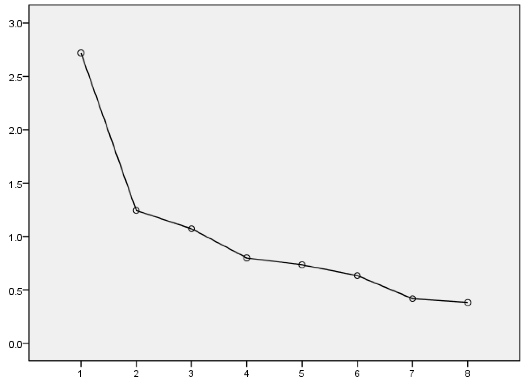
Table 1. Selected Indicators.

Variable	Indicator Name	Calculation Method
X1	Liquidity	(Current Assets - Current Liabilities) / Average Total Assets
X2	Profitability	Retained Earnings / Average Total Assets
X3	Leverage	Earnings Before Interest and Taxes / Average Total Assets
X4	Solvency	Equity Market Value / Total Liabilities
X5	Turnover	Operating Income / Average Total Assets
X6	Cash Flow	Net Cash Flow from Operating Activities / Current Liabilities
X7	Asset Growth	(Total Assets at End of Period - Total Assets at Beginning of Period) / Total Assets at Beginning of Period
X8	Profitability	(Operating Income - Operating Cost) / Operating Income
X9	Enterprise Nature	Private Enterprises: 0, State-owned Enterprises: 1
X10	Industry Classification	Manufacturing: 0, Non-manufacturing: 1

Table 2. Financial Indicator Data for ST (including *ST) and Non-ST A-share Listed Companies in 2020.

Code	600654	600093	002052	603322	......	000632	300310	600742	600103
X1	-0.1672	-0.2749	-0.0776	0.0658		0.0384	0.5093	0.0717	0.3632
X2	-0.4564	-0.7002	-1.7612	0.0536		0.032	-0.5171	0.2949	0.0974
X3	-0.0094	-0.9426	-0.1608	0.0508		0.0362	0.0048	0.0628	0.027
X4	0.492	0.6802	1.6943	1.6586		0.261	5.5492	0.6515	2.7525
X5	0.6	0.72	0.35	0.65		0.95	0.87	1.15	0.45
X6	0.0053	-0.0461	-0.0154	0.0549		-0.3073	0.0815	0.3261	0.0611
X7	-0.1454	-0.3738	0.2733	0.0225		0.0752	0.0009	0.1109	-0.0064
X8	0.0624	0.0061	0.1051	0.1976		0.0569	0.1329	0.0983	0.1349
X9	0	1	0	0		1	0	1	1
X10	1	1	0	1		1	1	0	0
Y	0	0	0	0		1	1	1	1

* Data sourced from TongHuaShun Finance financial statements. The ellipsis (...) indicates that the table has been truncated for brevity. The complete table would include all stock codes and corresponding indicator values.

Table 3. Descriptive Statistics of Indicator Data.

Indicator	Num	Min	Max	Mean	Variance
X1	320	-2.0559	0.882	0.106496	0.144
X2	320	-6.4172	0.6771	-0.229231	0.757
X3	320	-1.201	0.2227	-0.039178	0.035
X4	320	0.0495	46.2045	5.121727	49.429
X5	320	0	1.59	0.428313	0.094
X6	320	-1.3786	1.1797	0.104675	0.094
X7	320	-0.9561	3.077	0.016794	0.113
X8	320	-0.9251	1	0.235367	0.05
X9	320	0	1	0.203	0.162
X10	320	0	1	0.5	0.251

Table 4. Correlation Coefficients of Indicator Data.

	X1	X2	X3	X4	X5	X6	X7	X8	X9	X10
X1	1
X2	0.373	1
X3	0.425	0.316	1
X4	0.407	0.083	0.169	1
X5	0.237	0.199	0.304	-0.022	1
X6	0.174	0.351	0.28	0.168	0.224	1
X7	0.339	0.081	0.517	0.18	0.289	0.153	1
X8	0.307	0.167	0.279	0.262	-0.038	0.265	0.084	1
X9	-0.108	-0.008	-0.013	-0.112	0.069	-0.055	0.037	-0.151	1
X10	-0.048	0.006	-0.016	-0.02	-0.107	-0.002	0.05	0.05	-0.023	1

Table 5. Significance Analysis.

X1	X2	X3	X4	X5	X6	X7	X8	X9	X10
0.232	0	0.005	0.579	0	0.008	0.436	0.895	0.401	0.149

Table 6. KMO Measure and Bartlett's Test.

KMO Measure of Sampling Adequacy		0.684
Bartlett's Test of Sphericity	Approximate Chi-Square Value	486.096
	Degrees of Freedom	28
	Significance	0.000

Table 7. Eigenvalues and Contribution Values of Principal Components.

	Initial Eigenvalue			Extracted Sums of Squared Loadings			Rotated Sums of Squared Loadings
	Total	Variance%	Cumulative%	Total	Variance%	Cumulative%	Total	Variance%	Cumulative%
1	2.719	33.986	33.986	2.719	33.986	33.986	1.019	12.735	12.735
2	1.244	15.552	49.537	1.244	15.552	49.537	1.016	12.698	25.433
3	1.072	13.402	62.939	1.072	13.402	62.939	1.013	12.658	38.091
4	0.799	9.984	72.923	0.799	9.984	72.923	1.012	12.646	50.737
5	0.735	9.182	82.106	0.735	9.182	82.106	1.011	12.641	63.378
6	0.633	7.916	90.022	0.633	7.916	90.022	1.004	12.544	75.922
7	0.417	5.216	95.238	0.417	5.216	95.238	0.964	12.052	87.974
8	0.381	4.762	100	0.381	4.762	100	0.962	12.026	100
Extraction Method: Principal Component Analysis

Table 8. Rotated Factor Loadings.

Com	1	2	3	4	5	6	7	8
X1	0.15	0.213	0.185	0.11	0.143	0.042	0.914	0.168
X2	0.005	0.017	0.96	0.081	0.06	0.165	0.16	0.122
X3	0.265	0.056	0.142	0.138	0.133	0.116	0.17	0.91
X4	0.072	0.97	0.017	-0.03	0.115	0.071	0.178	0.048
X5	0.125	-0.029	0.079	0.971	-0.04	0.101	0.093	0.116
X6	0.054	0.072	0.163	0.103	0.122	0.964	0.038	0.099
X7	0.95	0.077	0.004	0.132	0.016	0.054	0.133	0.231
X8	0.017	0.115	0.059	-0.04	0.969	0.12	0.122	0.111
Extraction Method: Principal Component Analysis. Rotation Method: Kaiser Normalization with Varimax Rotation. a. The rotation converged after 6 iterations.

Table 9. Component Score Coefficient Matrix.

Com	1	2	3	4	5	6	7	8
X1	-0.113	-0.203	-0.179	-0.089	-0.113	0.041	1.247	-0.134
X2	0.07	0.032	1.125	-0.048	-0.014	-0.168	-0.207	-0.129
X3	-0.269	0	-0.11	-0.091	-0.112	-0.066	-0.133	1.258
X4	-0.059	1.097	0.033	0.065	-0.09	-0.071	-0.244	0.002
X5	-0.111	0.065	-0.049	1.087	0.081	-0.101	-0.106	0.107
X6	-0.029	-0.07	-0.171	-0.099	-0.119	1.105	0.049	-0.078
X7	1.166	-0.055	0.066	-0.104	0.033	-0.029	-0.126	-0.309
X8	0.036	-0.089	-0.014	0.08	1.093	-0.121	-0.132	-0.135

Table 10. Logistic Regression Coefficients.

Com	B	S.E.	Wald	df	Significance	Exp(B)
F1	0.724	0.183	15.684	1	0	2.062
F2	0.342	0.201	2.902	1	0.088	1.408
F3	2.919	0.509	32.857	1	0	18.521
F4	1.499	0.245	37.334	1	0	4.477
F5	0.456	0.239	3.649	1	0.056	1.578
F6	1.354	0.232	34.007	1	0	3.875
F7	1.135	0.241	22.231	1	0	3.11
F8	1.784	0.395	20.442	1	0	5.953
Constant	-0.613	0.248	6.104	1	0.013	0.542

Table 11. Evaluation of the Logistic Regression Model.

Observations		Estimate
		ST=0，Non ST=1		Percentage Correct
		0.0	1.0
ST=0，Non ST=1	0.0	143	17	89.4
	1.0	16	144	90.0
Overall Percentage				89.7

Table 12. Compare of Logistic Regression Model.

Observations		Estimate			Observations		Estimate
		ST=0，Non ST=1		Percentage Correct			ST=0，Non ST=1		Percentage Correct
		0.0	1.0				0.0	1.0
ST=0，Non ST=1	0.0	153	7	95.6	ST=0，Non ST=1	0.0	145	15	90.6
	1.0	77	83	51.9		1.0	45	115	71.9
Overall Percentage				73.8	Overall Percentage				81.3
a.Segmentation Threshold 0.887					a. Segmentation Threshold 0.754

Table 13. P-Value Correspondence Table.

Significance	95%	90%	89.4%
P-Value	0.887	0.754	0.5

Table 14. Divide Corresponding Table.

A-level: Significant Risk	P≤0.5	Z≤0
B-level: Moderate Risk	0.5＜P≤0.754	0＜Z≤1.12
C-level: Minor Risk	0.754＜P≤0.887	1.12＜Z≤2.06
D-level: No Risk	P＞0.887	Z＞2.06

Table 15. Divide Corresponding Table.

Observations		Estimate
		ST=0，Non ST=1		Percentage Correct
		0.0	1.0
ST=0，Non ST=1	0.0	28	2	93.3
	1.0	0	30	100.0
Overall Percentage				96.7

Disclaimer/Publisher’s Note: The statements, opinions and data contained in all publications are solely those of the individual author(s) and contributor(s) and not of MDPI and/or the editor(s). MDPI and/or the editor(s) disclaim responsibility for any injury to people or property resulting from any ideas, methods, instructions or products referred to in the content.

© 2024 by the authors. Licensee MDPI, Basel, Switzerland. This article is an open access article distributed under the terms and conditions of the Creative Commons Attribution (CC BY) license (http://creativecommons.org/licenses/by/4.0/).

Copyright: This open access article is published under a Creative Commons CC BY 4.0 license, which permit the free download, distribution, and reuse, provided that the author and preprint are cited in any reuse.

MDPI Initiatives

Important Links

Choose an area of interest and we will send you notifications of new preprints at your preferred frequency.

Disclaimer

Research on Financial Risk Management Early Warning Model for Chinese Enterprises

Abstract

1. Introduction

2. Related Literature

3. Model Research

3.1. Sample Source

3.2. Indicator Selection

3.3. Indicator Selection

3.4. Factor Analysis

3.5. Logistic Regression

3.6. Risk Level Classification

3.7. Testing and Validation

4. Definition of General Model

5. Conclusions

Author Contributions

Funding

Institutional Review Board Statement

Informed Consent Statement

Data Availability Statement

Conflicts of Interest

Disclaimer

References

MDPI Initiatives

Important Links

Subscribe