
Submitted:
07 May 2024
Posted:
08 May 2024
You are already at the latest version
Abstract
Spatial and temporal variation of the free electron concentration in the ionosphere affects SAR interferograms, in particular at low radar frequencies. In this work the identification, estimation and compensation of ionospheric path delay phases in PALSAR-3 and NISAR-L interferograms is discussed. Both these L-band sensors acquire simultaneously SAR data in a main spectral band and in an additional, spectrally separated, narrower second band to support the mitigation of ionospheric path delays. The methods presented permit separating the dispersive and the non-dispersive phase terms based on the double-difference interferogram between the two available spectral bands and the differential interferogram of the main band. The applicability of the proposed methods is demonstrated using PALSAR-3-like data that was simulated based on PALSAR-2 SM1 mode data.
Keywords:
SAR
; DInSAR
; ionosphere
; dispersive phase
; non-dispersive phase
; split-spectrum method
; double difference interferogram
; PALSAR-3
; NISAR
1. Introduction
SAR interferometry [1,2] has been successfully used for more than 20 years to create numerical elevation models [3] and to map terrain displacements, including seismic motion [4,5], volcanoes [6], landslides [7,8,9], and ice motion [10,11,12]. However, the interferometric phase not only contains information about ground geometry and displacement, but is also influenced by changes in tropospheric and ionospheric conditions [13]. The interferometric SAR phase can be expressed as a sum of phase components. The orbital phase, the topographic phase, the deformation phase, and the differential tropospheric path delay phase are linearly dependent on the radar frequency. The ionospheric path delay phase, or ionospheric phase for short, on the other hand, is indirectly proportional to the frequency and can be expressed as follows [14]
where ΔTEC is the difference between the Total Electron Content (TEC) values integrated along the line-of-sight of the two radar acquisitions, and K=40.31m3s-2 is a constant, c=3.0e8m/s is the speed of light and f0 is the radar center frequency. The ionospheric phase is dispersive (proportional to 1/f0). In this work on the identification and mitigation of ionospheric effects we do not call the dispersive phase, i.e. the phase term proportional to 1/f0, “ionosphere phase” or “ionospheric path delay phase”, as SAR data focusing using imperfect parameters is another possible cause for dispersive phase. Using a slightly wrong Doppler rate can result in an overall dispersive phase ramp.
The concept of the split-spectrum approach is to determine separate interferograms for spectral sub-bands, permitting separation of the dispersive and the non-dispersive phase terms ([14,15,16,17,18,19,20,21,22,23]). As compared to previous sensors PALSAR-3 [24] and NISAR-L [25] provide data in two separated spectral bands, a broader main spectral band and a narrower secondary spectral band. In Section 2, we first present the data used and then generalize the spectral diversity method so that it can be applied for both the single-band and dual-band cases. Furthermore, we also consider the method proposed in [26], namely, to express the dispersive and non-dispersive phases as a linear combination of the main interferogram phase and the double-difference interferogram phase, as this has significant advantages concerning the robustness and accuracy of the method. In Section 3, some processing related aspects are discussed, followed by the discussion of the results obtained using simulated PALSAR-3 data and the conclusions.
2. Materials and Methods
2.1. Simulation of PALSAR-3 SLC Data with Two Spectral Bands Based on PALSAR-2 SM1 Mode SLC Data
Using an interferometric pair of PALSAR-2 SM1 data over Osaka, with a bandwidth of 80 MHz, we simulated PALSAR-3 data with the characteristics as indicated in Table 1. We first applied band-pass filtering of the PALSAR-2 SM1 data with a 28 MHz and 10 MHz band-pass filters at the lower and higher end of the available 80 MHz chirp bandwidth. For each sub-band we applied then a center frequency change to shift the filtered signal band into the center of the spectrum and reduced the range sampling so that the available signal band corresponds to 80% of the sampling bandwidths. As a result, simulated SLCs were obtained, equivalent to the PALSAR-3 28 MHz and 10 MHz bands.
2.2. Adapting the Split-Spectrum Method to the PALSAR-3 and NISAR L-Band SAR Cases
In the split-spectrum approach at least two separate spectral bands are used. We name the corresponding center frequencies fL for the lower and fH higher frequency band. In addition, we use a third frequency f0 for the center frequency of the main frequency band, this is the frequency band of the interferometric analysis that is done after the estimation and mitigation of the ionospheric phase. In the case of data with a single frequency band f0 is typically the center frequency of the full frequency band. In the case of data with two separate frequency bands band f0 is the frequency of the main (broader) frequency band, which can be the lower or higher frequency band.
In our derivation the interferogram phases at the frequencies f0, fL and fH are called φ0, φL and φH and the related dispersive and non-dispersive components φiono,0, φiono,L, φiono,H, φnd,0, φnd,L and φnd,H. Considering the indirect and direct proportionality of the dispersive and non-dispersive phase terms we can write the following set of equations
Equations (2) can be transformed to express the dispersive and non-dispersive phase terms as a linear combinations of φL and φH
or as a linear combination of φ0 and (φH -φL)
For data with a single spectral band a quite common approach is to calculate spectral bands for the highest and lowest third of the processed chirp spectrum. For specific PALSAR-1 and PALSAR-2, PALSAR-3, and NISAR modes the resulting scaling factors are listed in Table 1. For PALSAR-1 and PALSAR-2 modes center frequencies of specific data we have access to are used. For PALSAR-3 the characteristics used were found in [24], for NISAR -L in [25].
The factors a, b, c and d are used to scale the phases of the differential interferograms in the lower and upper spectral band. To perform phase scaling with a non-integer factor, it is necessary that this phase has already been unwrapped. As can be seen from Table 1, the factors a, b, c and d are non-integer values that are significantly greater than 1. This is problematic as it upscales phase noise and phase errors from the spatial filtering applied to reduce noise and facilitate phase unwrapping.
Using Eqs. (3-4), requires scaling of the unwrapped phases with large factors. Even small phase errors or noise effects of 0.1 radian will be scaled up resulting in significant phase errors. Therefore, using Eqs. (5-6), i.e. the approach based on the main band interferogram phase and the double difference interferogram between the lower and higher spectral bands is preferred, as it makes the ionosphere mitigation more robust and accurate [26].
For the new sensors with an additional secondary frequency band (PALSAR-3, NISAR-L) the separation of the main and secondary frequency band is relatively large. The resulting factors z between 9 and 12, used to scale the unwrapped differential interferometric phase, are much smaller than in the case of a single frequency band, except for the 80MHz bandwidth PALSAR-2 SM1 mode data. The scaling of the split spectrum double difference phase with the factor z, which has comparable values to the a and b factors, is less critical. The phase is usually much smaller than a phase cycle, so that unwrapping becomes trivial. Strong spatial filtering to perform the unwrapping is therefore not necessary.
In all the investigated cases the scale factor for the phase of the differential interferogram of the main band, x, has values very close to 0.5. The relative deviations of x from 0.5 are < 3%, so replacing it with 0.50 results in scaling errors below 3%. Approximating x with 0.5 and multiplying both sides of Eq. (5) with 2 results in
In contrast to equation 5, equation 7 can also be applied to the complex-valued differential interferogram phase φ0, since no scaling of φ0 with a non-integer value is necessary. This means that we can determine a complex-valued image for twice the dispersive phase and only need to unwrap the double differential interferogram, which can be done by directly converting the complex values into phase values. On the one hand, this complex-valued image makes it possible to qualitatively determine the extent of the ionospheric effects. On the other hand, it can be unwrapped to quantify the relative ionospheric phase delays. For pairs with small ionospheric effects, which should be the vast majority of interferometric pairs, unwrapping 2φiono,0 should not be too difficult. In many cases, the phases will remain in the interval [-π,π], with respect to a reference near the center of the image, or they will vary along an almost linear phase ramp.
A complex-valued image of twice the non-dispersive phase can be calculated by subtracting twice the dispersive phase from twice the interferogram phase. Inserting twice the dispersive phase as expressed in Equation 7 results in
This means a complex version of twice the non-dispersive phase, or the “ionosphere-corrected” interferogram, can be generated without the need for phase unwrapping of the complex-valued differential interferogram φ0.
The main non-dispersive phase terms are deformation phase and tropospheric path delay phase, considering, that orbital and topographic phase terms are usually modeled and subtracted. Besides, there are error terms and phase noise.
Very often, and especially in L-band, the spatial variation of the non-dispersive phase is rather small. In cases with strong ionospheric phase effects, unwrapping the double non-dispersive phase can be much easier than unwrapping the original interferogram. An example where the dispersive phase is significantly larger than the non-dispersive phase is presented below. Cases with strong non-dispersive phases occur at displacements of more than one decimeter, caused for example by earthquakes, ice movements, and rapid landslides and subsidence.
In the following, we call the method based on Eq. 5 Method 1 (M1). M1 requires the calculation of the unwrapped split spectrum double-difference phase and the unwrapped phase of the differential interferogram. The great advantage of M1 is that the unwrapped phase is only scaled by a small factor of about 0.5, which greatly reduces the quality requirements regarding filtering. M1 does not require an approximation and uses the exact scaling factors.
The methods based on Eqs. 7 and 8 are called Methods 2 and 3 (M2, M3). The obvious advantage of M2 and M3 is that complex-valued images of twice the dispersive phase (M2) and twice the non-dispersive phase (M3) can be calculated, whereby only the split spectrum double difference phase has to be unwrapped. As already mentioned, this step is straightforward. Provided that the double dispersive phase or the double non-dispersive phase can be unwrapped, scaling is also possible to obtain the unwrapped dispersive and non-dispersive phases. It is helpful that often either the double dispersive phase or the double non-dispersive phase has only small values and is therefore easy to unwrap. As M2 and M3 use the same phase terms, we typically apply both methods.
2.3. Processing Related Aspects
2.3.1. Band-Pass Filtering
When using SLC data in a single frequency band band-pass filtering along the range spectrum axis, e.g. considering the lowest and highest third of the processed bandwidth, is applied to get two sub-band SLCs in a lower and higher spectral band. Here, in the case of simulated PALSAR-3 or NISAR-L data we consider SLC data sets that are already provided in two bands, a main band with a typically broader range bandwidth (e.g. 28 MHz in the case of PALSAR-3) and a secondary narrower band (10 MHz in the PALSAR-3 case). Consequently, no band-pass filtering is necessary in the mitigation of the dispersive phase.
2.3.2. Effects of the SLC co-Registration on the Interferogram
Gradients in the dispersive path delay along the synthetic aperture lead to azimuthal position deviations [27], which can be up to several SLC pixels for L-band images (see example below). If a co-registration method is used that is either based exclusively on the orbit data, the SAR processing parameters and a digital elevation model (DEM) or a method that is based on range and azimuth offset polynomials of low order, which are determined with the aid of matching techniques, an appropriate co-registration is obtained overall. However, local effects caused by the dispersion path delay gradients are not compensated. Registration errors larger than one pixel lead to a significant reduction in coherence. In addition, we have found that registration errors can also significantly affect the interferogram phase, as demonstrated by the example presented in Section 4.
Our co-registration procedure, which also includes a consideration of local effects, comprises a first step based on the orbit, the SAR parameters and a DEM, and a second step in which the remaining local offsets are determined using matching techniques. Taking into account the quality of the determined offsets and their spatial consistency, the offset field is conditioned. Outliers are removed, the offset field is interpolated in areas with poor coverage and then slightly spatially filtered. The resulting offset field is then used to refine the co-registration.
An iteration of this procedure or the use of the split-beam double difference phase may not be successful in the case of strong ionospheric gradients. Different parts of the azimuth spectrum of the SLC are affected by different parts of the ionosphere (as the relevant layer is located at a height of almost 300km above ground and is not on or near the ground).
Applying the co-registration with the offset field refinement results in a much-reduced split-beam interferogram (SBI) phase. But in areas with really high gradients there may still be a non-zero SBI phase and further refining the co-registration will also not fully correct this.
Conducting the same co-registration procedure with offset field refinements per azimuth sub-band and combining then the co-registered azimuth sub-band SLCs again into one full band SLC, results in a SBI with significant non-zero “ionosphere-like” phase streaks.
2.3.3. Interferogram Filtering and Unwrapping
Multi-looking and spatial filtering is used to reduce phase noise in interferograms and to support the necessary phase unwrapping step. Spatial filtering also allows the phase signal to be interpolated for small gaps, e.g. in areas with low coherence. Spatial filtering methods exist for both complex-valued and real-valued data sets. A commonly used method for filtering complex-valued interferograms is the Goldstein-Werner filter [28]. We use a modified version of it, which is available in the Gamma software [29]. We usually filter unwrapped phase images with a moving window filter with different filter sizes and weighting functions. For spatial phase unwrapping, we use a minimum cost flow (MCF) algorithm [30], where the interferometric coherence is taken into account in the calculation of the cost function [29].
It is also possible to iterate the phase unwrapping procedure, e.g. for interferograms with very large phase signals. An initial solution is generated using a stronger filter. It is important that the unwrapped phase does not show any phase jumps. This first solution is then subtracted from the original interferogram. The resulting complex-valued interferogram has less phase variation than the original interferogram. By repeating the filtering, unwrapping, and subtracting, the phase variation in the remaining complex-valued interferogram can be further reduced. As soon as the phase variation remains within the interval (-π,π), the complex-valued interferogram can be converted directly into a real-valued phase image. The unwrapped phase is then obtained by summing up the components from the individual iteration steps.
3. Results Using Simulated PALSAR-3 Data over Osaka
Using an interferometric pair of PALSAR-2 SM1 data over Osaka, with 80 MHz bandwidth, we simulated PALSAR-3 data with the characteristics as indicated in Table 2. Two subsequent scenes were concatenated to get a better spatial coverage of the ionospheric distortions present. The concatenation was done after the range band-pass filtering.
For the main band SLCs we conducted an ionosphere check for the single SLC, by determining the offset field between azimuth sub-band images (Figure 1). Pixel level azimuth offsets clearly identify the scene acquired on 20160601 as significantly affected by ionospheric effects.
For interferometric processing we used the earlier scene, i.e. the one without strong ionospheric effects, as the geometric reference. For comparison, we carried out the co-registration with and without an offset field refinement. The resulting differential interferograms are quite different (Figure 2). Differential interferograms calculated for smaller azimuth sub-bands look quite similar to the differential interferogram obtained with the co-registration with an offset field refinement. But the location of the strong phase gradients, which correspond to the location of the dispersive path delay gradients, differs depending on the squint angle of the selected azimuth sub-band, as the ionospheric effects occur at a significant height (e.g. 300km) above the ground surface. Summing up the azimuth sub-band differential interferogram phases partially cancels the really strong phase gradients. In the case of the co-registration with the offset field refinement the application of the offset field correction “corrects” the azimuth sub-band differential interferometric phases approximately to the differential interferometric phase in the zero Doppler geometry. The split-beam interferograms (SBI) calculated for the co-registered SLCs confirm this: only in the case of the co-registration without offset field refinement the SBI shows strong phase differences (Figure 3). Besides the different phase an important difference is the significantly higher coherence obtained with the offset field refinement co-registration.
Using the SLCs co-registered with an offset field refinement we then did the dispersive phase mitigation. Using Method 1 the unwrapped differential interferogram phase for the main band and the unwrapped double difference interferogram phase are used (Figure 4). Notice that the phases in the double difference interferogram are all within the same phase cycle – so that unwrapping was trivial. Applying Eq. (3) with the scaling factors x and z as listed in Table 1, the dispersive path delay was calculated. Figure 5 shows the PALSAR-3 main band differential interferogram, the estimated dispersive path delay phase and the resulting non-dispersive phase.
Then we also applied methods M2 and M3. Twice the dispersive path delay phase (Figure 6 left, M2) and twice the non-dispersive phase (Figure 6 right, M3) could be calculated without phase unwrapping, except for the trivial unwrapping of the double difference interferogram phase.
All 3 mitigation methods (M1, M2, M3) clearly indicate that the dominant, spatially varying part of the differential interferometric phase corresponds to ionospheric path delay. Considering, the azimuth offset fields (between the two scenes, but also between azimuth sub-bands of a single scene) and SBI tells us that the ionospheric effects are mainly present in the scene acquired on 20160601.
4. Discussion
Checking the simulated PALSAR-3 data for ionospheric effects worked well for three different methods applied. The calculation of the azimuth offset field between two azimuth sub-bands of a single SLC is a robust process that can be easily automated. An important advantage of this method is that it permits identifying ionospheric distortions in a single SLC. Considering the azimuth offsets of the co-registration offset field refinement also permitted identifying the presence of significant ionospheric effect. This method involves both the reference and the second scene. Consequently, it is not clear which of the two scenes (or both) is affected by ionospheric distortions. Calculating the co-registration refinement offset field is also suited to assess the quality of the co-registration, and it can also be automated easily. More difficult to automate is the conditioning of the refinement offset field (rejecting outliers, spatial filtering, and interpolation) needed to actually refine the co-registration. Using the split-beam interferogram is more delicate. If the SLC co-registration is done without offset-field refinement, the SBI phase clearly indicates the presence of ionospheric anomalies. But, if the co-registration was done with an offset field refinement the SBI phase is significantly reduced and does not indicate the presence of ionospheric anomalies with the same clarity.
Mitigating the ionospheric effects worked well for the simulated PALSAR-3 data used. Method 1 worked well as we were able to unwrap the differential interferometric phase. In Methods 2 and 3 the complex images for the double dispersive and the double non-dispersive phase could easily be obtained as no unwrapping was required except for the direct conversion of the complex values of the double difference interferogram to phase values. In cases with extreme ionospheric distortions the double difference phases may reach levels outside (-π,π). In this case it would be necessary to either unwrap the phase or the level of the values can be reduced by selecting two sub-bands with a reduced spectral separation. In the PALSAR-3 case this could be done by generating two sub-bands of the 28MHz bandwidth SLC.
Methods 2 and 3 should typically be both applied. Sometimes, as in the example shown, the ionospheric phase is the dominant phase term. So, unwrapping twice the ionospheric phase will be more challenging than unwrapping the original differential interferogram. Twice the non-dispersive phase, on the other hand, is more smooth and clearly simpler to unwrap than the original differential interferogram. In other cases with only small ionospheric distortions, it is exactly the opposite. Twice the dispersive phase will be smoother and therefore more easily unwrapped than the original differential interferogram, that may include substantial displacement phase.
The results obtained for simulated NISAR-L data correspond closely to those obtained for the simulated PALSAR-3 data and are therefore not shown.
5. Conclusions
The upcoming PALSAR-3 and NISAR-L both offer SAR acquisitions in a main frequency band complemented with a narrower secondary frequency band, to support the mitigation of ionospheric path delay effects. In preparation of the ionosphere mitigation in PALSAR-3 and NISAR-L data we generalized the mitigation techniques so that they can be applied to data with a single or with two separate frequency bands. Using PALSAR-2 SM1 data with a 80 MHz bandwidth we simulated PALSAR-3 and NISAR-L SLC data and tested the procedures to identify and mitigate ionospheric path delay effects.
Checking if ionospheric distortions affect the data can be done either for a single SLC or for an interferometric pair. For the investigated data the presence or absence of significant ionospheric effects, i.e. path delay phase effects and positional effects as a function of the azimuth spectral band, could reliably be identified for the individual SLCs determining positional offsets between azimuth sub-band images generated using band-pass filtering. The presence of ionospheric distortions could also be identified by calculating the split-beam interferogram, but only if the SLC of the second date was co-registered to the reference scene without offset field refinement. When applying an offset field refinement in the co-registration the split-beam interferogram doesn’t clearly show the presence of an ionospheric effects, but azimuth offsets at SLC pixel level in the refinement offset field clearly indicate the presence of ionospheric effects.
To minimize the processing complexity the mitigation method M1 uses the unwrapped phase of the main band differential interferogram and of the double difference interferogram. The challenging part in the processing is the phase unwrapping step for the differential interferogram. Keeping the scaling factor for this term low, around 0.5, is limiting the scaling up of spatial filtering effects and unwrapping errors. Unwrapping the phase of the double difference interferogram could be done by directly converting the complex values to phases, as the values were clearly within [-π,π].
Furthermore, M2 and M3 were successfully used to get complex valued interferograms with the phase corresponding to twice the dispersive phase and twice the non-dispersive phase. The spatial variation of the complex valued interferogram corresponding to twice the non-dispersive phase was quite smooth without high gradients (as for the dispersive phase) so that unwrapping it is less challenging. The complex valued interferogram corresponding to twice the dispersive phase clearly confirms the presence of strong ionospheric effects.
Author Contributions
“Conceptualization, U.W. and C.W.; methodology, all authors; software, C.W., C.M., and U.W.; validation, U.W. and C.M.; formal analysis, U.W. and O.F.; investigation, all authors; writing—original draft preparation, U.W.; writing—review and editing, O.F., C.W.; visualization, U.W., C.M.; supervision, U.W.; project administration, U.W.; funding acquisition, all authors. All authors have read and agreed to the published version of the manuscript.”
Funding
“This research received no external funding”.
Acknowledgments
PALSAR-2 original data copyright JAXA, obtained through research announcement project ER3A4N003.
Conflicts of Interest
“The authors declare no conflicts of interest.”
References
- Bamler, R.; Hartl, P. Synthetic aperture radar interferometry. Inverse Probl. 1998, 14, R1. [Google Scholar] [CrossRef]
- Rosen, P.; Hensley, S.; Joughin, I.; Li, F.; Madsen, S.; Rodriguez, E.; Goldstein, R. Synthetic aperture radar interferometry. Proc. IEEE 2000, 88, 333–382. [Google Scholar] [CrossRef]
- Zink, M.; Moreira, A. TanDEM-X mission status: The new topography of the earth takes shape. IEEE IGARSS 2014, pp. 3386-3389.
- Massonet, D.; Rossi, M.; Carmona, C.; Adragna, F.; Peltzer, G.; Feigl, K.; Rabaute, T. The displacement field of the Landers earthquake mapped by SAR interferometry, Nature 1993, 364, 138-142.
- Sato, H.P.; Harp, E.L. Interpretation of earthquake-induced landslides triggered by the 12 May 2008, M7.9 Wenchuan earthquake in the Beichuan area, Sichuan Province, China using satellite imagery and Google Earth. Landslides 2009, 6, 153–159. [Google Scholar] [CrossRef]
- Sandwell, D.T.; Myer, D.; Mellors, R.; Shimada, M.; Brooks, B.; Foster, J. Accuracy and Resolution of ALOS Interferometry: Vector Deformation Maps of the Father's Day Intrusion at Kilauea. IEEE Trans. Geosci. Remote. Sens. 2008, 46, 3524–3534. [Google Scholar] [CrossRef]
- Colesanti, C.; Wasowski, J. Investigating landslides with space-borne Synthetic Aperture Radar (SAR) interferometry. Eng. Geol. 2006, 88, 173–199. [Google Scholar] [CrossRef]
- Delacourt, C.; Allemand, P.; Berthier, E.; Raucoules, D.; Casson, B.; Grandjean, P.; Pambrun, C.; Varel, E. Remote-sensing techniques for analysing landslide kinematics: a review. BSGF - Earth Sci. Bull. 2007, 178, 89–100. [Google Scholar] [CrossRef]
- Strozzi, T.; Ambrosi, C.; Raetzo, H. Interpretation of Aerial Photographs and Satellite SAR Interferometry for the Inventory of Landslides. Remote. Sens. 2013, 5, 2554–2570. [Google Scholar] [CrossRef]
- Joughin, I.; Kwok, R.; Fahnestock, M. Estimation of ice-sheet motion using satellite radar interferometry: method and error analysis with application to Humboldt Glacier, Greenland, Journal of Glaciology 1996, 42-142.
- Goldstein, R.M.; Engelhardt, H.; Kamb, B.; Frolich, R.M. Satellite Radar Interferometry for Monitoring Ice Sheet Motion: Application to an Antarctic Ice Stream. Science 1993, 262, 1525–1530. [Google Scholar] [CrossRef] [PubMed]
- Mohr, J.J.; Reeh, N.; Madsen, S.N. Three-dimensional glacial flow and surface elevation measured with radar interferometry. Nature 1998, 391, 273–276. [Google Scholar] [CrossRef]
- Gray, A.L.; Mattar, K.E.; Sofko, G. Influence of ionospheric electron density fluctuations on satellite radar interferometry. Geophys. Res. Lett. 2000, 27, 1451–1454. [Google Scholar] [CrossRef]
- Meyer, F.; Bamler, R.; Jakowski, N.; Fritz, T. The Potential of Low-Frequency SAR Systems for Mapping Ionospheric TEC Distributions. IEEE Geosci. Remote. Sens. Lett. 2006, 3, 560–564. [Google Scholar] [CrossRef]
- Brcic, R.; Parizzi, A.; Eineder, M.; Bamler, R.; Meyer, F. Estimation and compensation of ionospheric delay for SAR interferometry. In Proceedings of the 2010 IEEE International Geoscience and Remote Sensing Symposium, Honolulu, HI, USA, 25–30 July 2010; pp. 2908–2911. [Google Scholar]
- Brcic, R.; Parizzi, A.; Eineder, M.; Bamler, R.; Meyer, F. Ionospheric effects in SAR interferometry: An analysis and comparison of methods for their estimation. In Proceedings of the 2011 IEEE International Geoscience and Remote Sensing Symposium, Vancouver, BC, Canada, 24–29 July 2011; pp. 1497–1500. [Google Scholar]
- Rosen, P.A.; Hensley, S.; Chen, C. Measurement and mitigation of the ionosphere in L-band Interferometric SAR data. In Proceedings of the 2010 IEEE Radar Conference; IEEE, Washington, DC, USA, 10–14 May 2010; pp. 1459–1463. [Google Scholar]
- Gomba, G.; De Zan, F. Estimation of ionospheric height variations during an aurora event using multiple semi-focusing levels. Procs. International Geoscience and Remote Sensing Symposium (IGARSS) 2015, pp. 4065–4068.
- Gomba, G.; Parizzi, A.; De Zan, F.; Eineder, M.; Bamler, R. Toward Operational Compensation of Ionospheric Effects in SAR Interferograms: The Split-Spectrum Method. IEEE Trans. Geosci. Remote. Sens. 2015, 54, 1446–1461. [Google Scholar] [CrossRef]
- Furuya, M.; Suzuki, T.; Maeda, J.; Heki, K. Midlatitude sporadic-E episodes viewed by L-band split-spectrum InSAR. Earth, Planets Space 2017, 69, 175. [Google Scholar] [CrossRef]
- Liao, H.; Meyer, F.J.; Scheuchl, B.; Mouginot, J.; Joughin, I.; Rignot, E. Ionospheric correction of InSAR data for accurate ice velocity measurement at polar regions. Remote. Sens. Environ. 2018, 209, 166–180. [Google Scholar] [CrossRef]
- Fattahi, H.; Simons, M.; Agram, P. InSAR Time-Series Estimation of the Ionospheric Phase Delay: An Extension of the Split Range-Spectrum Technique. IEEE Trans. Geosci. Remote. Sens. 2017, 55, 5984–5996. [Google Scholar] [CrossRef]
- Tymofyeyeva, E.; Fialko, Y. Mitigation of atmospheric phase delays in InSAR data, with application to the eastern California shear zone. J. Geophys. Res. Solid Earth 2015, 120, 5952–5963. [Google Scholar] [CrossRef]
- Information on PALSAR-3 Instrument. 2023, https://earth.esa.int/eogateway/documents/20142/2982981/10_191120SARwgcv_tadono. 1910.
- NASA-ISRO SAR (NISAR) Mission Science Users’ Handbook. https://nisar.jpl.nasa.gov/documents/26/NISAR_FINAL_9-6-19.
- Wegmüller, U.; Werner, C.; Frey, O.; Magnard, C.; Strozzi, T. Reformulating the Split-Spectrum Method to Facilitate the Estimation and Compensation of the Ionospheric Phase in SAR Interferograms. Procedia Comput. Sci. 2018, 138, 318–325. [Google Scholar] [CrossRef]
- Wegmuller, U.; Werner, C.; Strozzi, T.; Wiesmann, A. Ionospheric Electron Concentration Effects on SAR and INSAR. In Proceedings of the 2006 IEEE International Geoscience and Remote Sensing Symposium, Denver, CO, USA, 31 July–4 August 2006; pp. 3731–3734. [Google Scholar] [CrossRef]
- Goldstein, R.M.; Werner, C.L. Radar interferogram filtering for geophysical applications. Geophys. Res. Lett. 1998, 25, 4035–4038. [Google Scholar] [CrossRef]
- Gamma Software Information, 2018, at https://www.gamma-rs.ch/software.html.
- Costantini, M. A novel phase unwrapping method based on network programming. IEEE Trans. Geosci. Remote. Sens. 1998, 36, 813–821. [Google Scholar] [CrossRef]
Figure 1.
Azimuth offsets (in SLC pixels) between azimuth sub-band images for the first and last third of the azimuth spectrum. The pixel level offsets observed for the acquisition on 20160601 are a clear indication for ionospheric effects (dispersive path delay phase gradients along the synthetic aperture causing positional effects).
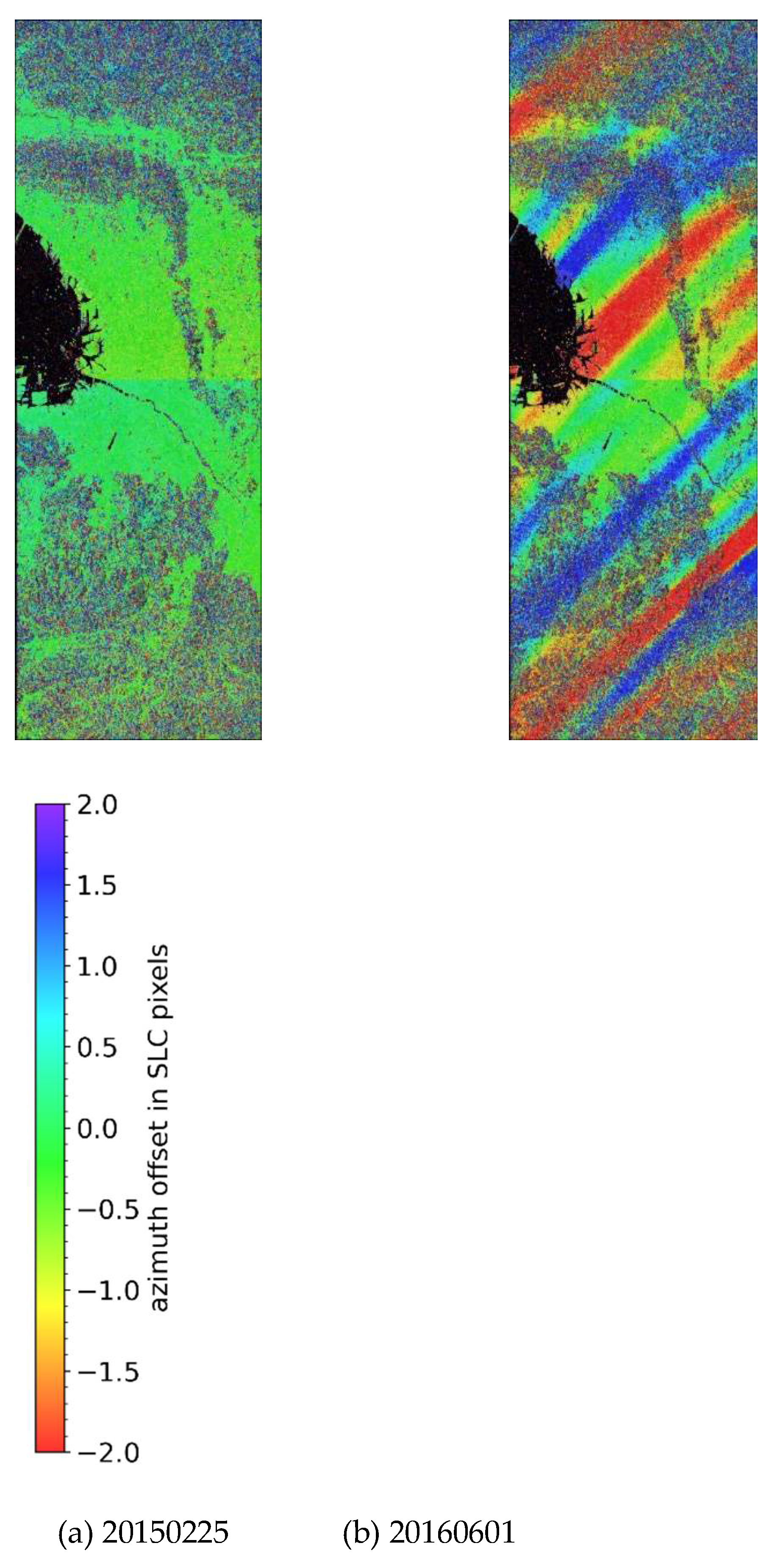
Figure 2.
Differential interferograms without (a) and with (b) offset field refinement in the co-registration step.
Figure 2.
Differential interferograms without (a) and with (b) offset field refinement in the co-registration step.
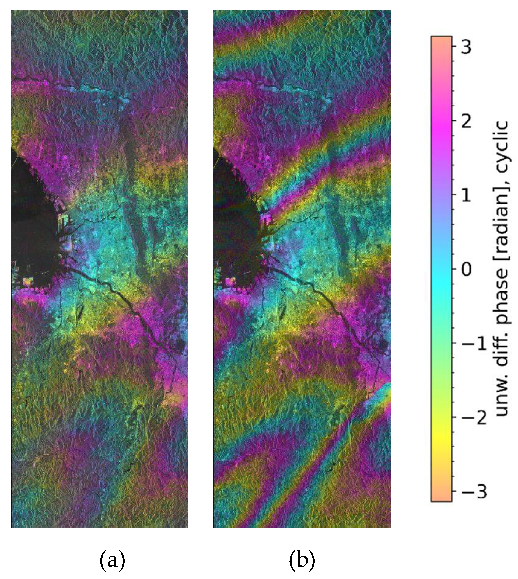
Figure 3.
Split-beam interferometric phase obtained for the SLCs co-registered without (a) and with (b) offset field refinement.
Figure 3.
Split-beam interferometric phase obtained for the SLCs co-registered without (a) and with (b) offset field refinement.
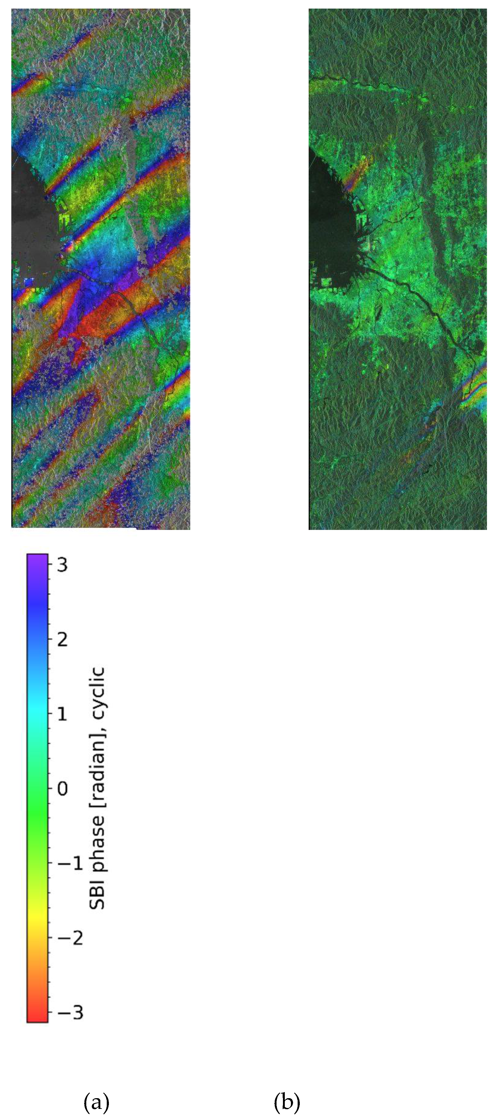
Figure 4.
Unwrapped differential interferogram phase for the 28 MHz band data (a) and unwrapped double difference interferogram phase (b).
Figure 4.
Unwrapped differential interferogram phase for the 28 MHz band data (a) and unwrapped double difference interferogram phase (b).
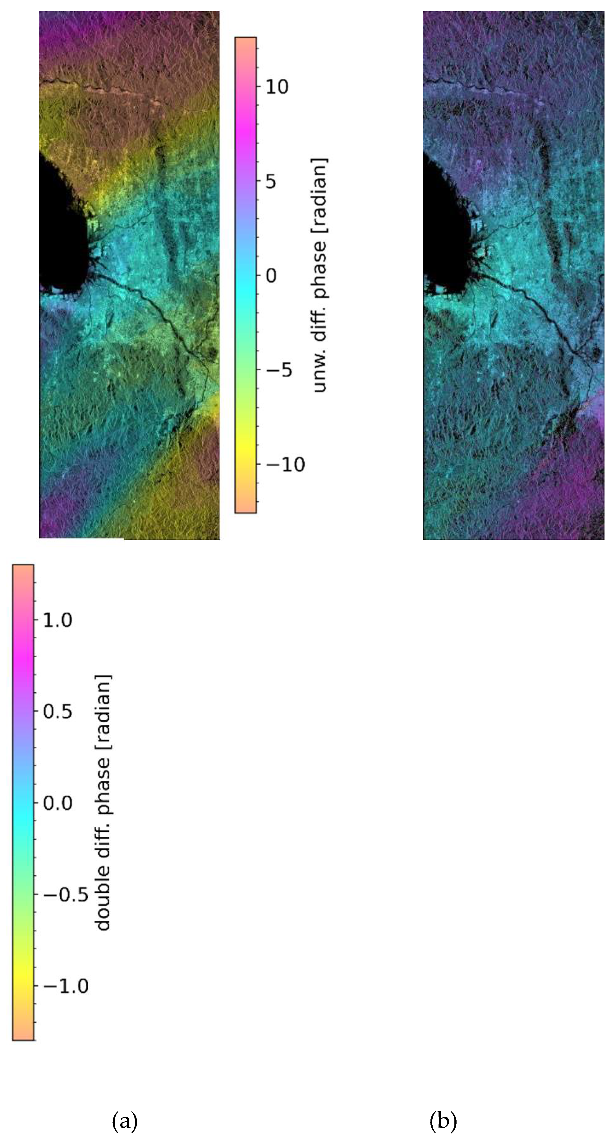
Figure 5.
Differential interferogram phase for the 28 MHz band (a), estimated dispersive phase delay phase (b), and non-dispersive or ionosphere-corrected phase (c), all using the cyclic color scale of Figure 6.
Figure 5.
Differential interferogram phase for the 28 MHz band (a), estimated dispersive phase delay phase (b), and non-dispersive or ionosphere-corrected phase (c), all using the cyclic color scale of Figure 6.
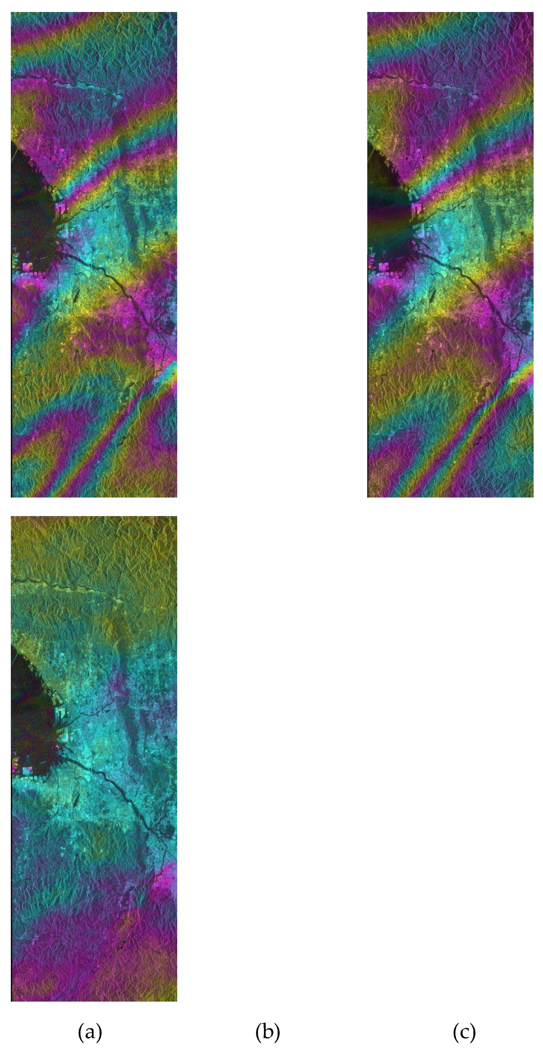
Figure 6.
Phase of complex valued images showing twice the dispersive path delay phase derived using M2 (a) and twice the non-dispersive phase derived using M3 (b), both calculated without phase unwrapping.
Figure 6.
Phase of complex valued images showing twice the dispersive path delay phase derived using M2 (a) and twice the non-dispersive phase derived using M3 (b), both calculated without phase unwrapping.
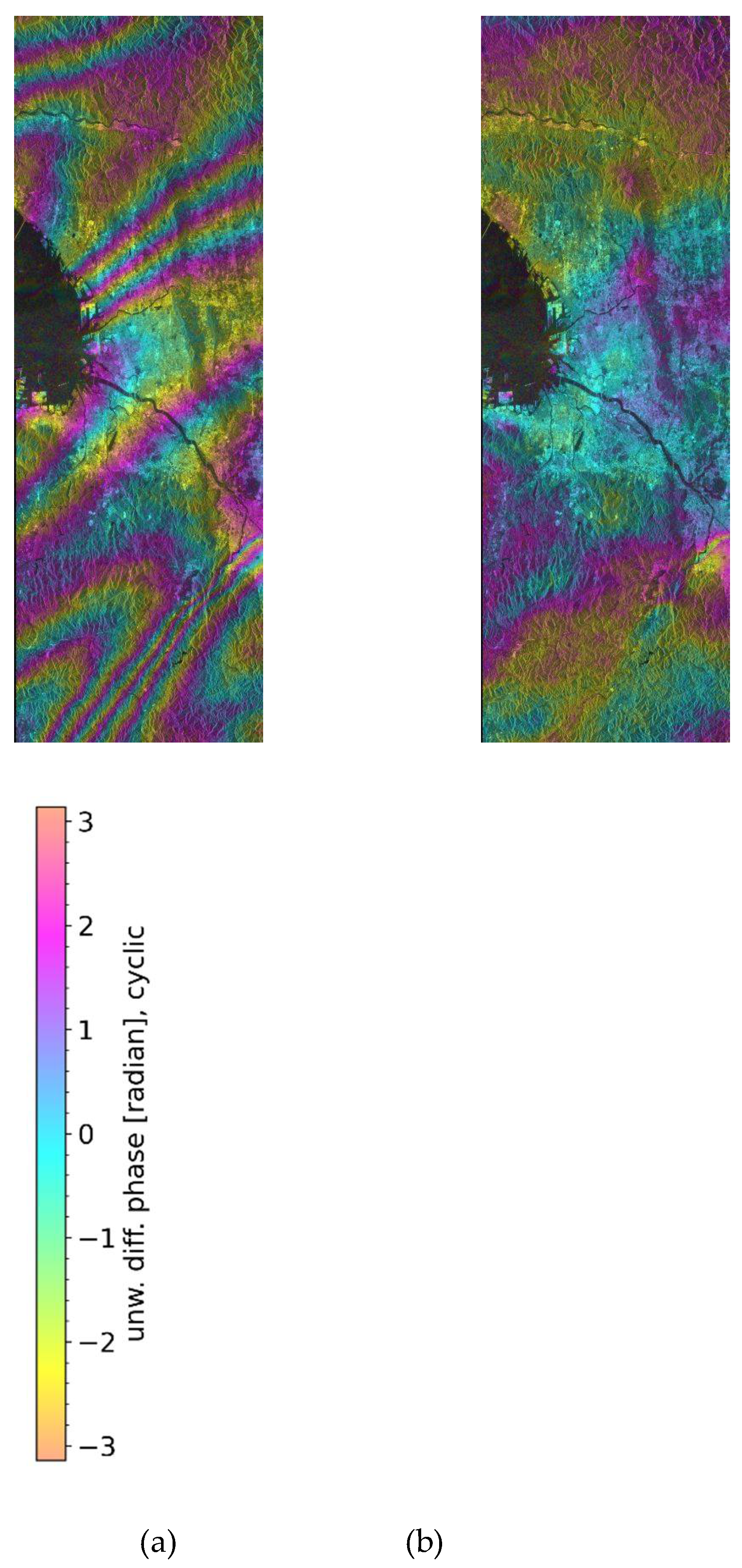

Table 1.
Factors a, b, c, d, x, and z used in Eqs. (3-6) to calculate the dispersive and non-dispersive phase components for different PALSAR-1, PALSAR-2, PALSAR-3, and NISAR-L modes. The center frequencies used in the calculations are indicated.
Table 1.
Factors a, b, c, d, x, and z used in Eqs. (3-6) to calculate the dispersive and non-dispersive phase components for different PALSAR-1, PALSAR-2, PALSAR-3, and NISAR-L modes. The center frequencies used in the calculations are indicated.
| Mode | f0[GHz] | fL[GHz] | fH[GHz] | a | b | c | d | x | z |
| PALSAR-3 28MHz | 1.2330 | 1.2330 | 1.2910 | 11.38 | -10.87 | -10.39 | 10.87 | 0.511 | -10.87 |
| NISAR L 20MHz | 1.2275 | 1.2275 | 1.2950 | 9.85 | -9.34 | -8.85 | 9.34 | 0.513 | -9.34 |
| NISAR L 40MHz | 1.2375 | 1.2375 | 1.2950 | 11.52 | -11.01 | -10.52 | 11.01 | 0.511 | -11.01 |
| PALSAR-1 14MHz | 1.2700 | 1.2653 | 1.2747 | 68.24 | -67.74 | -67.74 | 68.24 | 0.500 | -67.99 |
| PALSAR-1 28MHz | 1.2700 | 1.2607 | 1.2793 | 34.28 | -33.78 | -33.78 | 34.28 | 0.500 | -34.03 |
| PALSAR-2 12MHz | 1.2365 | 1.2325 | 1.2405 | 78.17 | -77.67 | -77.67 | 78.17 | 0.500 | -77.92 |
| PALSAR-2 25MHz | 1.2700 | 1.2617 | 1.2783 | 38.50 | -38.00 | -38.00 | 38.50 | 0.500 | -38.25 |
| PALSAR-2 80MHz | 1.2575 | 1.2310 | 1.2840 | 12.12 | -11.62 | -11.62 | 12.12 | 0.500 | -11.88 |
Disclaimer/Publisher’s Note: The statements, opinions and data contained in all publications are solely those of the individual author(s) and contributor(s) and not of MDPI and/or the editor(s). MDPI and/or the editor(s) disclaim responsibility for any injury to people or property resulting from any ideas, methods, instructions or products referred to in the content. |
© 2024 by the authors. Licensee MDPI, Basel, Switzerland. This article is an open access article distributed under the terms and conditions of the Creative Commons Attribution (CC BY) license (http://creativecommons.org/licenses/by/4.0/).
Copyright: This open access article is published under a Creative Commons CC BY 4.0 license, which permit the free download, distribution, and reuse, provided that the author and preprint are cited in any reuse.


