Reappraising Double Pendulum Dynamics across Multiple Computational Platforms

This study presents the complexity and sensitivity of chaotic system dynamics in the case of the double pendulum. It applied detailed numerical analyses of the double pendulum in multiple computing platforms in order to demonstrate the complexity in behavior of the system of double pendulums. The equations of motion were derived from the Euler-Lagrange formalism, in order to capture the system's dynamics, which is coupled nonlinearly. These were solved numerically using the efficient Runge-Kutta-Fehlberg method, implemented in Python, R, GNU Octave, and Julia, while runtimes and memory usage were extensively benchmarked across these environments. Time series analyses, including the calculation of Shannon entropy and the Kolmogorov-Smirnov test, quantified the system's unpredictability and sensitivity to infinitesimal perturbations of the initial conditions. Phase space diagrams illustrated the intricate trajectories and strange attractors, as further confirmation of the chaotic nature of the double pendulum. All the findings have a clear indication of the importance of accurate measurements of the initial condition in a chaotic system, contributing to an increased understanding of nonlinear dynamics. Future research directions are faster simulations using Numba and GPU computing, stochastic effects, chaotic synchronization, and applications in climate modeling. This work will be useful for understanding chaos theory and efficient computational approaches in complex systems of dynamical nature.

Keywords:

Subject: Computer Science and Mathematics - Applied Mathematics

1. Introduction

The double pendulum forms an interesting physics system consisting of two pendululum hanging in a rigidly connected line. It does not only rely on the observation of immediate effects but also the study of the underlying structures that make things change. Though at first glance this machine may look mundane, its behavior will prove to be exciting and the underlying idea of balance between order and disorder that has intrigued scientists and mathematicians for centuries will be inspirationally brought to life. It is an example of the fascinating ways simple systems can exhibit complex behavior. From people like Henri Poincaré, who first took a look at non-linear systems and laid the foundation for chaos theory, to today’s powerful computational models, the double pendulum remains a symbol that the secret of nonlinear dynamics is a profound one [1].

A double pendulum consists of two massless rods, each with a concentrated point mass at its end, connected by a frictionless hinge. This seemingly simple setup actually displays a remarkable sensitivity to initial conditions, a characteristic of chaotic systems that was first discovered by British mathematician and physicist Mary Cartwright in the early 20th century [1,2]. Even tiny changes in the starting position can cause significant divergences in the paths the system takes - a concept that challenges the traditional idea put forth by French scholar Pierre-Simon Laplace known as Laplace’s demon, which suggests that knowing all initial conditions of a system guarantees the ability to predict its future evolution with total certainty [3].

The double pendulum is a prominently studied dynamical system in climate science due to its exquisite sensitivity to initial conditions, making it a valuable model for studying chaos theory and its applications in understanding Earth’s complex climate systems [4]. Gaining insights into chaotic systems like the double pendulum could prove vital for tackling one of our most pressing global issues - anthropogenic climate change driven by human activities. Several studies have used simplified models like the double pendulum to gain insights into the non-linear dynamics underlying atmospheric-oceanic flows and long-range climate predictions [5,6,7,8,9].

The double pendulum exemplifies how deterministic systems can exhibit unpredictable, chaotic behavior, bridging the gap between the simple, ordered world of classical physics and the apparent randomness we observe in complex phenomena like weather and climate patterns [10]. This chaotic complexity represents a major frontier in our scientific understanding - we have robust theories for simple systems and stochastic models for randomness, but lack a unified framework to explain the rich dynamical behaviors that emerge in between the two extremes [11]. Unraveling the chaos inherent in multi-scale systems like the double pendulum may unlock deeper insights into the fundamental laws governing our climate and the universe at large.

In this paper, our main goal is to thoroughly investigate and analyze the complex movements of a double pendulum system using detailed numerical simulations. We utilized open-source computing platforms to develop engaging visuals that can be used as effective educational resources. This graphical representation will help students, especially those with limited abstract mathematics knowledge, better understand the concepts of calculus of variations. The calculus of variations is a branch of mathematical analysis concerned with optimizing functionals, which are mappings from a space of functions to the real numbers. It addresses problems where the goal is to find a function that extremizes a given functional, either minimizing or maximizing it [12]. This field is particularly important in areas such as physics, engineering, and economics, where one seeks to optimize quantities that depend on functions, such as energy, action, or cost [13]. By presenting this information visually and in a practical context, we hope to make it easier for students to connect theoretical concepts with real-world applications.

Furthermore, allowing students to freely access the simulation code enables them to explore the computational side of the project, enhancing their comprehension of how theory translates into practice. This also gives them the opportunity to improve and perfect the models, promoting a practical approach to learning physics and applied mathematics through coding. To ensure optimal performance and efficiency, we thoroughly evaluated the free and open-source computing environments utilized in this study. This study will offer helpful information for teachers, scholars, and professionals, helping them choose the best tools for their individual computing requirements and improving resource management and promoting excellence in scientific computing.

2. Methods

In order to predict the positional paths of two point masses in a double pendulum system, we need a classical mechanics framework represented by the Euler-Lagrange equation. This is because the Euler-Lagrange equation provides a systematic approach to deriving the equations of motion for complex systems like the double pendulum, taking into account the constraints and forces involved. On the other hand, using Newtonian mechanics alone for the double pendulum can be challenging due to the system’s nonlinear nature and the presence of constraints such as the lengths of the pendulum arms. While it’s possible to analyze simpler pendulum systems using Newton’s laws directly, the double pendulum’s motion involves coupled, nonlinear differential equations that are more conveniently handled using the Euler-Lagrange formalism [14].

The Euler-Lagrange equation is essential in classical mechanics and field theory, describing the motion of particles or fields by minimizing a functional known as the action. To derive this equation from scratch, we started with the action S, defined as the integral of the Lagrangian

(L)

over time:

S = \int_{t_{1}}^{t_{2}} L (q, \dot{q}, t) d t

(1)

Here, q represents the generalized coordinates,

\dot{q}

is the derivative of q with respect to time, and t is time. The Lagrangian

(L)

has a simple and concise definition:

L \equiv T - V

(2)

The kinetic energy (T) and potential energy (V) together make up the classical Lagrangian, which is just the difference between these energies in the system. This applies to classical mechanics with conservative systems, where the total energy is the sum of kinetic and potential energies. Our next step was to find the path

q (t)

that keeps the action constant, even if the path changes a little. This basic idea is called the principle of least action.

To find this stationary path, we used the calculus of variations. Let

δ q (t)

be a small variation in the path

q (t)

, such that

q (t)

becomes

q (t) + δ q (t)

. The variation in the action is then:

δ S = \int_{t_{1}}^{t_{2}} [L (q + δ q, \dot{q} + δ \dot{q}, t) - L (q, \dot{q}, t)] d t

(3)

We expanded

L (q + δ q, \dot{q} + δ \dot{q}, t)

in a Taylor series around q and

\dot{q}

L (q + δ q, \dot{q} + δ \dot{q}, t) = L (q, \dot{q}, t) + \frac{\partial L}{\partial q} δ q + \frac{\partial L}{\partial \dot{q}} δ \dot{q} + O (δ q^{2}, δ {\dot{q}}^{2})

(4)

Substituting the expression back into equation 3 we would consider terms up to second order or higher in

δ q

and

δ \dot{q}

in the variation of the action S,

O (δ q^{2}, δ {\dot{q}}^{2})

δ S = \int_{t_{1}}^{t_{2}} [\frac{\partial L}{\partial q} δ q + \frac{\partial L}{\partial \dot{q}} δ \dot{q}] d t + O (δ q^{2}, δ {\dot{q}}^{2})

(5)

Integrating the first term by parts with respect to t and assuming that variations

δ q (t_{1})

and

δ q (t_{2})

vanish (boundary conditions), we got:

δ S = \int_{t_{1}}^{t_{2}} [\frac{d}{d t} (\frac{\partial L}{\partial \dot{q}}) - \frac{\partial L}{\partial q}] δ q d t

(6)

For the action to be stationary,

δ S

must be zero for all possible variations

δ q

. This leads to the Euler-Lagrange equation:

\frac{d}{d t} (\frac{\partial L}{\partial \dot{q}}) - \frac{\partial L}{\partial q} = 0

(7)

This equation governs the dynamics of the system and provides the equations of motion for the generalized coordinates

q (t)

To apply the Euler-Lagrange equation to the double pendulum system, we must first establish its Lagrangian, which encapsulates both the system’s kinetic and potential energies. This process started by delineating the geometric relationships governing the vertical and horizontal positions within the double pendulum system, as illustrated in Figure 1. These relationships were formalized through the following equations, denoted as equations 8 and 9:

\begin{matrix} x_{1} = L_{1} sin (θ_{1}) \\ x_{2} = x_{1} + L_{2} sin (θ_{2}) \end{matrix}

(8)

\begin{matrix} y_{1} = L_{1} cos (θ_{1}) \\ y_{2} = y_{1} + L_{2} cos (θ_{2}) \end{matrix}

(9)

Here,

x_{1}

and

x_{2}

represent the horizontal positions, while

y_{1}

and

y_{2}

represent the vertical positions. These positions are determined by the lengths of the pendulum arms (

L_{1}

and

L_{2}

) and the angles (

θ_{1}

and

θ_{2}

Since the positions x and y are functions of the angles

θ_{1}

and

θ_{2}

, respectively, obtaining their first derivatives requires applying the chain rule. This application results in the following expressions:

\begin{matrix} {\dot{x}}_{1} = L_{1} {\dot{θ}}_{1} cos (θ_{1}) \\ {\dot{x}}_{2} = L_{1} {\dot{θ}}_{1} cos (θ_{1}) + L_{2} {\dot{θ}}_{2} cos (θ_{2}) \end{matrix}

(10)

\begin{matrix} {\dot{y}}_{1} = - L_{1} {\dot{θ}}_{1} sin (θ_{1}) \\ {\dot{y}}_{2} = - L_{1} {\dot{θ}}_{1} sin (θ_{1}) - L_{2} {\dot{θ}}_{2} cos (θ_{2}) \end{matrix}

(11)

These derivatives

{\dot{x}}_{1}, {\dot{x}}_{2}, {\dot{y}}_{1},

and

{\dot{y}}_{2}

represent the rates of change of the horizontal and vertical positions with respect to time, taking into account the angular velocities

{\dot{θ}}_{1}

and

{\dot{θ}}_{2}

Starting from the general formula for kinetic energy

T = \frac{1}{2} m v^{2}

(where m is the total of two-point masses of

m_{1} + m_{2}

and v is velocity), we substituted the velocities

{\dot{x}}_{1}, {\dot{x}}_{2}, {\dot{y}}_{1},

and

{\dot{y}}_{2}

from the systems of equations 10 and 11 into equation 12. This substitution yields the expanded form:

\begin{matrix} T & = \frac{1}{2} (m_{1} ({\dot{x}}_{1}^{2} + {\dot{y}}_{1}^{2}) + m_{2} ({\dot{x}}_{2}^{2} + {\dot{y}}_{2}^{2})) \\ = \frac{1}{2} (m_{1} {(L_{1} {\dot{θ}}_{1} cos (θ_{1}))}^{2} + m_{1} {(- L_{1} {\dot{θ}}_{1} sin (θ_{1}))}^{2} \\ + m_{2} {(L_{1} {\dot{θ}}_{1} cos (θ_{1}) + L_{2} {\dot{θ}}_{2} cos (θ_{2}))}^{2} + m_{2} {(- L_{1} {\dot{θ}}_{1} sin (θ_{1}) - L_{2} {\dot{θ}}_{2} cos (θ_{2}))}^{2}) \end{matrix}

(12)

Expanding and simplifying each term step by step, we obtained expressions for the kinetic energy components. These components involve terms related to the masses

m_{1}

and

m_{2}

, the lengths

L_{1}

and

L_{2}

of the pendulum arms, and the angular velocities

{\dot{θ}}_{1}

and

{\dot{θ}}_{2}

. After combining and simplifying the terms, we arrived at the final form of the kinetic energy:

T = \frac{1}{2} (m_{1} + m_{2}) L_{1}^{2} {\dot{θ}}_{1}^{2} + \frac{1}{2} m_{2} L_{2}^{2} {\dot{θ}}_{2}^{2} + m_{2} L_{1} L_{2} {\dot{θ}}_{1} {\dot{θ}}_{2} cos (θ_{1} - θ_{2})

(13)

This expression captures the kinetic energy T of the double pendulum system comprehensively, incorporating the masses

m_{1}

and

m_{2}

, the lengths

L_{1}

and

L_{2}

of the pendulum arms, and the angular velocities

{\dot{θ}}_{1}

and

{\dot{θ}}_{2}

in a way that reflects the system’s dynamics and interactions.

Beginning with equation 14, which defines potential energy as a function of the vertical positions

y_{1}

and

y_{2}

, and the gravitational constant g, we can express it as:

V = m_{1} g y_{1} + m_{2} g y_{2}

(14)

Substituting the expressions for

y_{1}

and

y_{2}

from the system of equations 9 into the above equation yields:

V = m_{1} g (L_{1} cos (θ_{1})) + m_{2} g (L_{1} cos (θ_{1}) + L_{2} cos (θ_{2}))

(15)

We then simplified this expression to:

V = g ((m_{1} + m_{2}) L_{1} cos (θ_{1}) + m_{2} L_{2} cos (θ_{2}))

(16)

Finally, to express potential energy V solely in terms of the angles

θ_{1}

and

θ_{2}

, we derived:

V = - g ((m_{1} + m_{2}) L_{1} cos (θ_{1}) + m_{2} L_{2} cos (θ_{2}))

(17)

Here, g represents the gravitational acceleration, and the potential energy V is derived from the vertical positions of the pendulum components and their respective masses, articulated in terms of the angles

θ_{1}

and

θ_{2}

After deriving the expressions for kinetic energy T and potential energy V, we can now formulate the Lagrangian

L

for the double pendulum system. The Lagrangian is defined in the definition 2. Substituting the expressions we derived for T and V into this equation, we obtained:

\begin{matrix} L & = \frac{1}{2} (m_{1} + m_{2}) L_{1}^{2} {\dot{θ}}_{1}^{2} + \frac{1}{2} m_{2} L_{2}^{2} {\dot{θ}}_{2}^{2} + m_{2} L_{1} L_{2} {\dot{θ}}_{1} {\dot{θ}}_{2} cos (θ_{1} - θ_{2}) \\ - (- g ((m_{1} + m_{2}) L_{1} cos (θ_{1}) + m_{2} L_{2} cos (θ_{2}))) \\ = \frac{1}{2} (m_{1} + m_{2}) L_{1}^{2} {\dot{θ}}_{1}^{2} + \frac{1}{2} m_{2} L_{2}^{2} {\dot{θ}}_{2}^{2} + m_{2} L_{1} L_{2} {\dot{θ}}_{1} {\dot{θ}}_{2} cos (θ_{1} - θ_{2}) \\ + g ((m_{1} + m_{2}) L_{1} cos (θ_{1}) + m_{2} L_{2} cos (θ_{2})) \end{matrix}

(18)

This expression for the Lagrangian

L

encapsulates the dynamic behavior of the double pendulum system. It incorporates the masses

m_{1}

and

m_{2}

, the lengths

L_{1}

and

L_{2}

of the pendulum arms, the angular velocities

{\dot{θ}}_{1}

and

{\dot{θ}}_{2}

, and the gravitational constant g, as well as the angles

θ_{1}

and

θ_{2}

that describe the positions of the pendulum components. The Lagrangian

L

serves as a fundamental quantity in the analysis of the system’s motion and dynamics, providing a comprehensive representation of its energy and interactions.

Starting with the Lagrangian

L

derived earlier (equation 18), we applied the Euler-Lagrange equation (equation 7) to derive the equations of motion for a system with two point masses (the double pendulum in this case). The Euler-Lagrange equation for a variable

q_{i}

is given by:

\frac{d}{d t} (\frac{\partial L}{\partial {\dot{q}}_{i}}) - \frac{\partial L}{\partial q_{i}} = 0

(19)

Applying this equation to the variables

θ_{1}

and

θ_{2}

separately, we obtained two set of equations:

\begin{matrix} \frac{d}{d t} (\frac{\partial L}{\partial \dot{θ_{1}}}) - \frac{\partial L}{\partial θ_{1}} = 0 \\ \frac{d}{d t} (\frac{\partial L}{\partial \dot{θ_{2}}}) - \frac{\partial L}{\partial θ_{2}} = 0 \end{matrix}

(20)

For

θ_{1}

, we first calculated the partial derivative of

L

with respect to

{\dot{θ}}_{1}

\frac{\partial L}{\partial {\dot{θ}}_{1}} = (m_{1} + m_{2}) L_{1}^{2} {\dot{θ}}_{1} + m_{2} L_{1} L_{2} {\dot{θ}}_{2} cos (θ_{1} - θ_{2})

(21)

Then, we took the derivative of this with respect to time t:

\frac{d}{d t} (\frac{\partial L}{\partial {\dot{θ}}_{1}}) = (m_{1} + m_{2}) L_{1}^{2} {\ddot{θ}}_{1} + m_{2} L_{1} L_{2} {\ddot{θ}}_{2} cos (θ_{1} - θ_{2})

(22)

Next, we calculated the partial derivative of

L

with respect to

θ_{1}

\frac{\partial L}{\partial θ_{1}} = - m_{2} L_{1} L_{2} {\dot{θ}}_{1} {\dot{θ}}_{2} sin (θ_{1} - θ_{2}) - g (m_{1} + m_{2}) L_{1} sin (θ_{1})

(23)

Finally, substituting these derivatives into the Euler-Lagrange equation (equation 20) for

θ_{1}

(m_{1} + m_{2}) L_{1}^{2} {\ddot{θ}}_{1} + m_{2} L_{1} L_{2} {\ddot{θ}}_{2} cos (θ_{1} - θ_{2}) = 0

(24)

To derive the equation of motion for

θ_{2}

using the Euler-Lagrange equation (equation 20), we started by calculating the partial derivative of the Lagrangian

L

with respect to the derivative of

θ_{2}

, denoted as

{\dot{θ}}_{2}

. This yields:

\frac{\partial L}{\partial {\dot{θ}}_{2}} = m_{2} L_{2}^{2} {\dot{θ}}_{2} + m_{2} L_{1} L_{2} {\dot{θ}}_{1} cos (θ_{1} - θ_{2})

(25)

Taking the time derivative of this expression gave us:

\frac{d}{d t} (\frac{\partial L}{\partial {\dot{θ}}_{2}}) = m_{2} L_{2}^{2} {\ddot{θ}}_{2} + m_{2} L_{1} L_{2} {\ddot{θ}}_{1} cos (θ_{1} - θ_{2}) - m_{2} L_{1} L_{2} {\dot{θ}}_{1} {\dot{θ}}_{2} sin (θ_{1} - θ_{2})

(26)

Next, we calculated the partial derivative of

L

with respect to

θ_{2}

, denoted as

\frac{\partial L}{\partial θ_{2}}

, which was given by:

\frac{\partial L}{\partial θ_{2}} = - m_{2} L_{1} L_{2} {\dot{θ}}_{1} {\dot{θ}}_{2} sin (θ_{1} - θ_{2}) - m_{2} L_{2} g sin (θ_{2})

(27)

Substituting the expressions for

\frac{\partial L}{\partial {\dot{θ}}_{2}}

and

\frac{\partial L}{\partial θ_{2}}

into the Euler-Lagrange equation and simplifying this equation further results in the equation of motion for

θ_{2}

, given as:

m_{2} L_{2} {\ddot{θ}}_{2} + m_{2} L_{1} {\ddot{θ}}_{1} cos (θ_{1} - θ_{2}) - m_{2} L_{1} {\dot{θ}}_{1}^{2} sin (θ_{1} - θ_{2}) + m_{2} g sin (θ_{2}) = 0

(28)

Combining the final forms of the Euler-Lagrange equations for

θ_{1}

(equation 24) and

θ_{2}

(equation 28) together form the complete system of equations of motion for the double pendulum system. They are coupled second-order ordinary differential equations (ODEs) because the acceleration terms

{\ddot{θ}}_{1}

and

{\ddot{θ}}_{2}

are dependent on each other due to the cosine and sine terms involving

θ_{1}

and

θ_{2}

. This coupling reflects the interdependence of the pendulum’s motions and positions, making the system dynamically rich and challenging to analyze without numerical or advanced analytical techniques.

For the numerical analysis, we substituted the following expressions

({\dot{θ}}_{1} = ω_{1}, {\dot{θ}}_{2} = ω_{2}, Δ θ = θ_{1} - θ_{2})

to simplify the system of equations for computational purposes. Substituting these into the given equations (equations 24 and 28), we obtained the following system:

\begin{matrix} (m_{1} + m_{2}) L_{1} {\dot{ω}}_{1} + m_{2} L_{2} {\dot{ω}}_{2} cos (Δ θ) + m_{2} L_{2} ω_{2}^{2} sin (Δ θ) + (m_{1} + m_{2}) g sin θ_{1} = 0 \\ m_{2} L_{2} {\dot{ω}}_{2} + m_{2} L_{1} {\dot{ω}}_{1} cos (Δ θ) - m_{2} L_{1} ω_{1}^{2} sin (Δ θ) + m_{2} g sin (θ_{2}) = 0 \end{matrix}

(29)

This transformed system allows us to numerically solve for the angular frequencies

ω_{1}

and

ω_{2}

given initial conditions and system parameters.

To simplify the numerical analysis, we first rewrote the original system of equations in terms of the defined variables:

\{\begin{matrix} α = (m_{1} + m_{2}) L_{1} \\ β = m_{2} L_{2} cos (Δ θ) \\ γ = m_{2} L_{1} cos (Δ θ) \\ δ = m_{2} L_{2} \\ ε = - m_{2} L_{2} ω_{2}^{2} sin (Δ θ) - m_{2} g sin (θ_{2}) \\ ζ = m_{2} L_{2} ω_{1}^{2} sin (Δ θ) - m_{2} g sin (θ_{2}) \end{matrix}

(30)

We then rewrote the system of equations in matrix form:

(\begin{matrix} α & β \\ γ & δ \end{matrix}) (\begin{matrix} {\dot{ω}}_{1} \\ {\dot{ω}}_{2} \end{matrix}) = (\begin{matrix} ε \\ ζ \end{matrix})

(31)

Finally, solving for

{\dot{ω}}_{1}

and

{\dot{ω}}_{2}

, we obtained:

\begin{matrix} {\dot{ω}}_{1} = \frac{ε δ - β ζ}{α δ - β γ} \\ {\dot{ω}}_{2} = \frac{α ζ - γ ε}{α δ - β γ} \end{matrix}

(32)

These derived equations were expressed in terms of the defined variables, providing a more organized and manageable representation for the numerical experiments.

For the numerical simulation needs in this study, we used parameters consistent with the physical properties of the system. These include an acceleration due to gravity (g) of

9.8 {m / s}^{2}

, the lengths of the pendulum arms

L_{1}

and

L_{2}

set to 2 meters and 1 meter respectively, and the masses of the pendulums (

m_{1}

and

m_{2}

) set at 1 kilogram and 2 kilograms respectively. The simulation time

(t)

is chosen to be 10 seconds with 10,000 linearly time spacing, providing sufficient duration to observe the system’s behavior.

With these parameters established, we set the initial conditions for the simulation. The initial angles (

θ_{1}

and

θ_{2}

) are set to 3.14 radians (which is equivalent to

180^{\circ}

) for

θ_{1}

and 1.57 radians (equivalent to

90^{\circ}

) for

θ_{2}

. Additionally, the initial angular velocities (

ω_{1}

and

ω_{2}

) are initialized to 0 radians per second, representing a starting point where the pendulums are at rest. For the subsequent simulation, we changed the both angular velocities to

0.001

radians per seconds fo the sensitivity test with the initial conditions.

We used the Runge-Kutta-Fehlberg (RKF) method for approximating the solution of our problem (system of equations 32). RKF is a powerful numerical integration technique used to solve systems of ODEs with high accuracy and computational efficiency [13]. Its adaptability makes it particularly suitable for dynamic systems like the double pendulum, where the motion can be complex and highly nonlinear.

We started with the initial conditions and set the initial step size h. Then, we proceeded to define the predictor step by using the 4th order Runge-Kutta formulas to predict the solution at the next time step. For a general ODE of the form

\frac{d y}{d t} = f (t, y)

, the 4th order Runge-Kutta formulas are:

\begin{matrix} k_{1} = h f (t_{n}, y_{n}) \\ k_{2} = h f (t_{n} + \frac{h}{2}, y_{n} + \frac{k_{1}}{2}) \\ k_{3} = h f (t_{n} + \frac{h}{2}, y_{n} + \frac{k_{2}}{2}) \\ k_{4} = h f (t_{n} + h, y_{n} + k_{3}) \end{matrix}

(33)

The predicted solution at

t_{n + 1}

is then given by:

y_{n + 1}^{(4)} = y_{n} + \frac{1}{6} (k_{1} + 2 k_{2} + 2 k_{3} + k_{4})

(34)

We used the 5th order Runge-Kutta formulas to compute a more accurate estimate of the solution at the next time step. The 5th order Runge-Kutta formulas are similar to the 4th order ones but include an additional evaluation point:

\begin{matrix} k_{1} = h f (t_{n}, y_{n}) \\ k_{2} = h f (t_{n} + \frac{h}{4}, y_{n} + \frac{k_{1}}{4}) \\ k_{3} = h f (t_{n} + \frac{3 h}{8}, y_{n} + \frac{3 k_{1}}{32} + \frac{9 k_{2}}{32}) \\ k_{4} = h f (t_{n} + \frac{12 h}{13}, y_{n} + \frac{1932 k_{1}}{2197} - \frac{7200 k_{2}}{2197} + \frac{7296 k_{3}}{2197}) \\ k_{5} = h f (t_{n} + h, y_{n} + \frac{439 k_{1}}{216} - 8 k_{2} + \frac{3680 k_{3}}{513} - \frac{845 k_{4}}{4104}) \\ k_{6} = h f (t_{n} + \frac{h}{2}, y_{n} - \frac{8 k_{1}}{27} + 2 k_{2} - \frac{3544 k_{3}}{2565} + \frac{1859 k_{4}}{4104} - \frac{11 k_{5}}{40}) \end{matrix}

(35)

The corrected solution at

t_{n + 1}

is then given by:

y_{n + 1}^{(5)} = y_{n} + \frac{1}{90} (7 k_{1} + 32 k_{3} + 12 k_{4} + 32 k_{5} + 7 k_{6})

(36)

Then, we calculated the local truncation error by comparing the 4th and 5th order solutions. The error estimate

ϵ_{n}

is given by:

ϵ_{n} = | y_{n + 1}^{(5)} - y_{n + 1}^{(4)} |

(37)

We compared the error estimate

ϵ_{n}

to a predefined tolerance. If

ϵ_{n}

is within the tolerance, accept the step and update the solution. If

ϵ_{n}

exceeds the tolerance, reduce the step size h and we repeated the process until the error is acceptable. Finally, we continued integrating until reaching the desired end time or number of steps.

The adaptive step-size control implemented in the RKF method ensures accurate integration while minimizing computational costs. By dynamically adjusting the step size based on error estimation, the RKF method provides accurate numerical approximations of the system’s behavior over time, rendering it an effective tool for analyzing complex dynamic systems such as the double pendulum. However, in the present study, we did not employ the RKF method directly from the beginning. Instead, we utilized several platform-specific tools, including SciPy in Python [15], deSolve in R [16], DifferentialEquations.jl in Julia [17], and the built-in function ode45 in GNU Octave [18].

The motivation behind using multiple programming languages and their respective computing environments was twofold. First, it allowed us to leverage the strengths and unique features of each language and environment, enabling a comprehensive exploration of the double pendulum problem from diverse perspectives. Second, it facilitated a comparative analysis of the performance and accuracy of different numerical solvers across these platforms.

In Python, the SciPy library provided a robust and well-established collection of scientific computing tools, including numerical solvers for ODEs. The flexibility and ease of use of Python, combined with the power of SciPy, made it a suitable choice for implementing and testing numerical methods for the double pendulum problem [19,20]. However, the interpreted nature of Python may introduce performance overhead compared to compiled languages.

The R programming language, with its deSolve package, offered a specialized environment for solving ODEs and differential algebraic equations (DAEs) [21]. R’s strong emphasis on statistical analysis and data visualization made it an attractive option for exploring the double pendulum problem, enabling efficient data analysis and visual representation of the results. Nonetheless, the high-level nature of R may lead to performance limitations for computationally intensive simulations.

Julia, a relatively new language designed for scientific computing, provided a high-performance computing environment through its DifferentialEquations.jl package. The combination of Julia’s dynamic programming capabilities and its efficient just-in-time (JIT) compilation made it a promising choice for solving the double pendulum problem with potentially improved computational performance [22,23]. However, the relatively young ecosystem of Julia may present challenges in terms of package maturity and community support.

Finally, GNU Octave, a high-level language primarily intended for numerical computations, offered the built-in ode45 function, which implements a versatile Runge-Kutta method for solving ODEs. GNU Octave’s compatibility with MATLAB^® syntax and its open-source nature made it an accessible option for researchers and students alike [18]. However, its performance may be limited compared to lower-level languages or specialized numerical libraries. By employing these various computing environments, we aimed to evaluate the trade-offs between performance, accuracy, and ease of use for each approach.

When conducting scientific research involving computational simulations, it is crucial to ensure reproducibility and transparency in the methods used. In this particular study, we aim to benchmark the performance of four different computing environments: Python, R, Octave/MATLAB, and Julia, by running a script that simulates the motion of a double pendulum. The script was executed 1,000 times in each computing environment, and the runtime and memory usage for each run will be measured and recorded. The benchmarking was performed on a Fedora Linux 39 (Budgie) x86_64 system with a 20LB0021US ThinkPad P52s laptop equipped with an Intel i7-8550U (8) @4.000GHz CPU.

The rationale behind this benchmarking approach is multifaceted. Firstly, it promotes reproducibility by providing the scripts and the benchmarking script, allowing other researchers to easily replicate the computational experiments and verify the results. Additionally, it facilitates a direct comparison of the runtime and memory usage across different computing environments for the same task, providing valuable insights into the relative performance of each environment. This information can guide researchers in choosing the most suitable tool for their specific computational needs.

Furthermore, running the scripts 1,000 times in each environment helps to account for potential variability and ensures that the performance measurements are consistent and reliable. This is particularly important when dealing with computationally intensive simulations like the double pendulum simulation, where minor fluctuations in hardware or software configurations can impact the results. With a large number of runs, it becomes possible to perform statistical analysis on the collected data, such as calculating confidence intervals, identifying outliers, and determining the statistical significance of any observed performance differences.

Measuring memory usage alongside runtime can provide insights into the scalability and resource requirements of each computing environment. This information is crucial when working with large-scale simulations or data-intensive applications, where efficient memory management is essential. By including the benchmarking methodology and results in the scientific paper, researchers demonstrate transparency and allow others to critically evaluate the computational approaches used in the study [24]. This aligns with the principles of open science and facilitates future replication and extension of the research.

After conducting the benchmarking process and collecting the runtime and memory usage data for each computing environment, we performed statistical analyses to determine if there were significant differences in performance among the platforms. Specifically, we employed the Kruskal-Wallis (K-W) test and Dunn’s test with Bonferroni adjustment, which are commonly used in various scientific fields for comparing multiple groups or treatments.

The K-W test is a non-parametric alternative to the one-way analysis of variance (ANOVA) and is used when the assumptions of normality and homogeneity of variances are violated [25]. It is a rank-based test that evaluates whether the populations from which the samples were drawn have the same distribution. The test statistic for the K-W test was calculated as:

H = \frac{12}{N (N + 1)} \sum_{i = 1}^{k} \frac{R_{i}^{2}}{n_{i}} - 3 (N + 1),

(38)

where N is the total number of observations across all groups, k is the number of groups,

R_{i}

is the sum of ranks for group i, and

n_{i}

is the number of observations in group i. The null hypothesis for the K-W test is that the populations have the same distribution, while the alternative hypothesis is that at least one population has a different distribution from the others.

If the K-W test indicates significant differences among the groups, post-hoc tests are typically performed to determine which specific groups differ from each other. In our case, we used Dunn’s test with Bonferroni adjustment, which is a multiple comparison procedure that adjusts the significance level to control the family-wise error rate (FWER) [26]. The Dunn’s test statistic for comparing groups i and j was calculated as:

Z = \frac{R_{i} - R_{j}}{\sqrt{\frac{N (N + 1)}{12} (\frac{1}{n_{i}} + \frac{1}{n_{j}})}}

(39)

, where

R_{i}

and

R_{j}

are the average ranks for groups i and j, respectively, N is the total number of observations across all groups, and

n_{i}

and

n_{j}

are the number of observations in groups i and j, respectively. The Bonferroni adjustment was applied by dividing the desired significance level (

α

) by the number of pairwise comparisons made, resulting in an adjusted significance level of

α / (\binom{k}{2})

, where k is the number of groups.

The K-W test and Dunn’s test with Bonferroni adjustment are widely used in various scientific fields [27,28,29]. These tests are particularly useful when dealing with non-normal data or when the assumptions of parametric tests (such as ANOVA) are violated. They provide a robust and reliable way to compare multiple groups or treatments, ensuring that any observed differences are statistically significant and not due to chance alone. By applying these statistical tests to our benchmarking data, we aimed to determine if there were significant differences in performance among the four computing environments (Python, R, GNU Octave, and Julia) for the double pendulum simulation task. These non-parametric procedures were implemented in Python using the SciPy stats module [15] and the scikit-posthoc library [30].

After conducting the benchmarking process to measure the runtime and memory usage of the double pendulum simulation across different computing environments, we further analyzed the obtained time series data to gain insights into the underlying dynamics of the system. One of the analysis techniques we employed was the calculation of Shannon entropy [31], which is a measure derived from information theory that quantifies the amount of information or uncertainty present in a random variable or time series. The Shannon entropy was calculated using the following equation:

H (X) = - \sum_{i = 1}^{n} p (x_{i}) {log}_{2} p (x_{i})

(40)

, where

H (X)

is the Shannon entropy, n is the number of unique values in the time series, and

p (x_{i})

is the probability of the occurrence of the value

x_{i}

in the time series. A higher Shannon entropy value indicates a higher degree of uncertainty or unpredictability in the time series, while a lower entropy value suggests a more predictable or regular pattern. This measure can provide valuable insights into the complexity and dynamics of the double pendulum system.

In our analysis, we calculated the Shannon entropy for each variable (e.g.,

x_{1}

y_{1}

θ_{1}

θ_{2}

ω_{1}

ω_{2}

) in the time series data obtained from the double pendulum simulation. To interpret the entropy scores, we established thresholds based on the following criteria: low entropy (predictable) for entropy scores

\leq 0.5

, medium entropy (some predictability) for entropy scores between 0.5 and 1.0, and high entropy (unpredictable) for entropy scores

> 1.0

. These thresholds are commonly used in various applications and provide a convenient way to interpret the degree of predictability or uncertainty present in the time series data. By calculating and analyzing the Shannon entropy of the time series data, we can gain insights into the predictability and complexity of the double pendulum system’s dynamics. A high entropy score for a particular variable suggests that the corresponding time series is highly unpredictable or complex, while a low entropy score indicates a more regular or predictable pattern.

The choice of Shannon entropy as an analysis technique was motivated by its strong theoretical foundation in information theory and its widespread use in various scientific fields for quantifying the complexity and uncertainty of dynamical systems. Furthermore, the interpretation of entropy scores based on predefined thresholds provides a convenient and standardized way to categorize the time series data into different levels of predictability or complexity.

After conducting the entropy measurement, we employed the Kolmogorov-Smirnov (K-S) test to assess the sensitivity of the system to initial conditions, which is a characteristic feature of chaotic systems. The K-S test is a non-parametric statistical test that compares the cumulative distribution functions (CDFs) of two samples to determine if they are drawn from the same underlying distribution [32]. In the context of dynamical systems analysis, the K-S test can be used to compare the time series obtained from the original system with slightly perturbed initial conditions, allowing us to quantify the divergence between the trajectories. Let

F (x)

and

G (x)

be the empirical CDFs of the original time series and the perturbed time series, respectively. The K-S statistic is defined as the maximum absolute difference between these two CDFs:

D_{n, m} = sup_{x} | F (x) - G (x) |

(41)

, where

{sup}_{x}

represents the supremum (least upper bound) of the set of absolute differences between the CDFs over all possible values of x.

The null hypothesis for the K-S test is that the two samples are drawn from the same continuous distribution, while the alternative hypothesis is that they are drawn from different distributions. The null hypothesis is rejected if the K-S statistic

D_{n, m}

exceeds a critical value that depends on the chosen significance level and the sample sizes n and m. In our analysis, we compared the original time series

(x_{1}, y_{1}, θ_{1}, θ_{2}, ω_{1}, ω_{2})

obtained from the double pendulum simulation with slightly perturbed time series, where the initial conditions for

ω_{1}

and

ω_{2}

were perturbed by 0.001 rad/s. By applying the K-S test to each pair of original and perturbed time series, we can assess whether the small perturbation in the initial conditions leads to a significant divergence in the trajectories over time. If the K-S test rejects the null hypothesis, indicating that the original and perturbed time series are drawn from different distributions, it suggests that the double pendulum system is sensitive to initial conditions, which is a hallmark of chaotic behavior. Conversely, if the test fails to reject the null hypothesis, it implies that the system is less sensitive to small perturbations in the initial conditions, suggesting a more predictable or regular dynamics.

The choice of the K-S test was motivated by its nonparametric nature, which means that it does not make assumptions about the underlying distribution of the data, making it suitable for analyzing complex dynamical systems where the distribution is often unknown or difficult to model parametrically. Additionally, the K-S test is widely used in various scientific fields for comparing distributions and detecting deviations from a hypothesized distribution [33,34,35], further justifying its application in our analysis. We employed SciPy’s stats module [15] to conduct an automated K-S test.

3. Results and Discussion

The K-W test, a non-parametric test for comparing multiple groups, yielded a test statistic of 3523.203 and a p-value of 0.000 for the runtime data, indicating that at least one group’s median runtime significantly differs from the others. Dunn’s post-hoc test, with Bonferroni adjustment for multiple comparisons, showed that all pairs of groups had p-values below 0.05, indicating significant differences in their median runtimes.

The results (Figure 2) indicate that R and GNU Octave exhibited the fastest runtimes, with mean values of 1.914 seconds and 1.944 seconds, respectively. The fast performance of R can be attributed to the use of the deSolve package, which provides efficient solvers for ODEs. GNU Octave, on the other hand, likely leverages optimized numerical libraries or solvers for ODE systems. Python followed closely with a mean runtime of 2.503 seconds, benefiting from the SciPy and NumPy libraries, which provide efficient numerical computations and ODE solvers. Notably, Julia had the slowest runtime performance, with a mean of 35.701 seconds, which is significantly longer than the other environments. One potential factor contributing to Julia’s slower performance could be the overhead associated with its JIT compilation process. JIT compilation can introduce additional runtime overhead, particularly for computationally intensive tasks like solving ODEs, which may have impacted Julia’s overall runtime performance in this specific implementation.

The K-W test for memory usage data yielded a test statistic of 3375.563 and a p-value of 0.000, indicating that at least one group’s median memory usage significantly differs from the others. Dunn’s post-hoc test showed that the pairs of groups with p-values below 0.05, indicating significant differences in their median memory usage, were GNU Octave-Julia, GNU Octave-Python, Julia-Python, and Julia-R. The results (Figure 2) show that Python, R, and GNU Octave exhibited similar memory usage patterns, with a mean of approximately 142.84 MB. Julia, on the other hand, had significantly higher memory usage, with a mean of 1031.703 MB, which is about seven times higher than the other environments. The differences in memory usage across the computing environments can be attributed to various factors, such as the memory management strategies of the respective programming languages and the specific implementation of the double pendulum simulation in each environment. However, it is worth noting that the pure Julia implementation using DifferentialEquations.jl may have different memory requirements or optimization strategies compared to the packages or libraries used in the other environments.

When selecting the appropriate computing environment for the double pendulum simulation, the statistical significance of the runtime and memory usage differences should be considered alongside other factors, such as existing codebase, familiarity with the language, and potential optimizations. If runtime performance is the primary concern, R and GNU Octave would be the recommended choices based on the provided results, with R leveraging the deSolve package and GNU Octave likely utilizing optimized numerical libraries or solvers for ODE systems. Python, with the SciPy and NumPy libraries, also exhibited a relatively good runtime performance and could be a viable option, especially if existing Python code or familiarity with the language is a consideration. If memory usage is a critical factor and the higher memory footprint of Julia is not a concern, Julia could be considered, potentially with further optimization efforts or alternative implementations. It is important to note that the pure Julia implementation using DifferentialEquations.jl may have different memory requirements or optimization strategies compared to the packages or libraries used in the other environments.

Figure 3 and Figure 4 present time series plots of a double pendulum system with slightly different initial angular velocities for the inner and outer pendulum. Each subplot displays the time evolution of the angular positions of both pendulums over 10 seconds with 1000 time steps.

The sensitivity to initial conditions is evident as the trajectories diverge significantly, despite only a small difference of 0.001 rad/s in the initial angular velocities (

ω_{1}

and

ω_{2}

) of the inner and outer pendulums. This phenomenon is characteristic of chaotic systems, where minuscule changes in initial conditions can lead to vastly different long-term behaviors, making precise predictions challenging [1]. The time series exhibit intricate patterns with recurring oscillations, indicative of the underlying nonlinear dynamics. However, the trajectories quickly diverge, showcasing the system’s sensitivity to initial conditions, a hallmark of chaos theory [36]. The time series initially following similar paths but rapidly diverging due to the infinitesimal differences in the initial angular velocities, further demonstrating the sensitive dependence on initial conditions in chaotic systems.

These results highlight the importance of accurately measuring and accounting for initial conditions in chaotic systems, as even minute uncertainties can amplify over time, leading to substantial deviations in the system’s behavior. The double pendulum serves as a compelling example of the intricate dynamics and unpredictability that can arise in nonlinear systems due to their extreme sensitivity to initial conditions, a fundamental concept in chaos theory [37].

To further quantify and statistically validate this divergence, we performed the K-S test on the time series data for various variables, including positions (x, y,

θ

) and angular velocities

(ω_{1}, ω_{2})

, before and after the initial perturbation. The K-S test results revealed that for each of these variables, the distributions of the time series data before and after the perturbation were significantly different, with p-values less than 0.05, leading to the rejection of the null hypothesis. This statistically confirms that the slight change in the initial angular velocity has a profound impact on the system’s dynamics, causing the distributions of the position and velocity variables to diverge substantially.

This divergence can be attributed to the chaotic nature of the double pendulum system, where the nonlinear equations governing its motion exhibit extreme sensitivity to initial conditions. Even minuscule differences in the starting values can rapidly amplify over time, leading to vastly different trajectories in the phase space [36]. The K-S test results corroborate this fundamental characteristic of chaos, demonstrating that the distributions of the system’s variables become statistically distinct due to the exponential divergence of initially close trajectories, a phenomenon known as the "butterfly effect" [38].

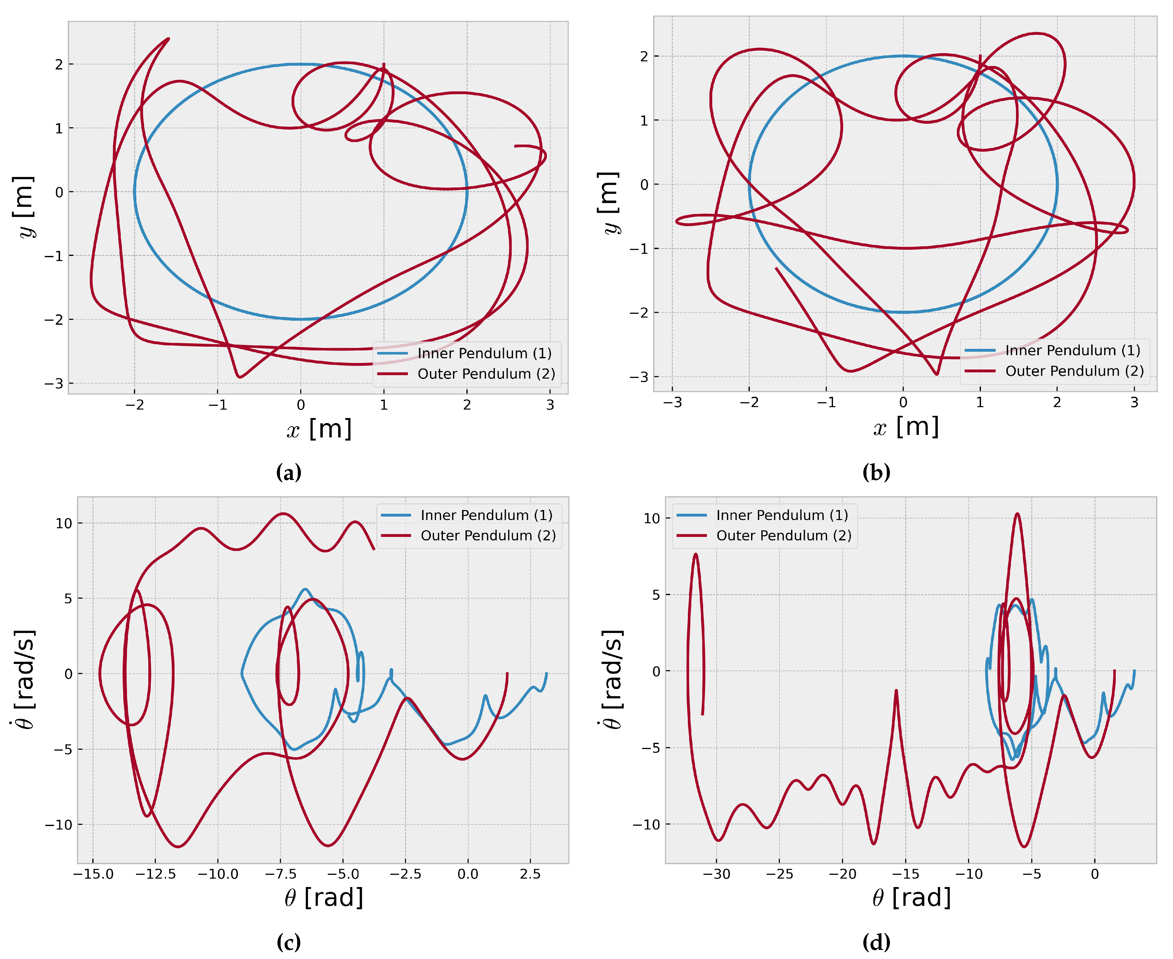
Figure 5 and Figure 5 show the trajectories of the inner and outer pendulums in the

x - y

plane, providing a visualization of their motion over time. However, Figure 5 and Figure 5 represent the phase space diagrams of the coupled pendulum system. A phase space diagram is a powerful tool for studying dynamical systems, as it provides a geometric representation of the system’s state at any given time [13]. In the case of the coupled pendulum system, the phase space diagrams plot the angular position

(θ)

of each pendulum against its angular velocity

(ω)

, capturing the evolution of the system’s state over time.

The complex patterns observed in Figure 5 and Figure 5 are indicative of the chaotic nature of the coupled pendulum system. The phase space trajectories exhibit intricate, aperiodic behavior, never repeating the same pattern or revisiting the same state. The presence of chaos in the coupled pendulum system has significant consequences for its predictability and controllability [36]. Even with precise knowledge of the initial conditions and governing equations, the system’s behavior becomes increasingly difficult to predict over long time scales due to the exponential divergence of nearby trajectories in the phase space.

Furthermore, chaotic systems often exhibit strange attractors in the phase space, which are geometrically complex structures that the system’s trajectories are confined. The presence of strange attractors in the phase space diagrams of the coupled pendulum system suggests that the system’s dynamics are governed by an underlying deterministic process, despite the apparent randomness and unpredictability of its behavior [1].

The high Shannon entropy values (greater than 1.0) mentioned for the time series data of the coupled pendulum system are consistent with the observed chaotic dynamics. For chaotic systems, the Shannon entropy is expected to be high due to the inherent unpredictability and lack of regularity in the system’s behavior [39].

4. Conclusions

The double pendulum system serves as a compelling example of the intricate dynamics and unpredictability that can arise in nonlinear systems due to their extreme sensitivity to initial conditions, a fundamental concept in chaos theory. Through numerical simulations and extensive analysis, we have demonstrated the chaotic behavior of the double pendulum, characterized by the exponential divergence of trajectories, the presence of strange attractors in the phase space, and high Shannon entropy values. These findings underscore the importance of accurately measuring and accounting for initial conditions in chaotic systems, as even minute uncertainties can amplify over time, leading to substantial deviations in the system’s behavior. Furthermore, our comparative study of different computing environments (Python, R, GNU Octave, and Julia) has revealed significant differences in their runtime performance and memory usage for the double pendulum simulation task. This information can guide researchers in selecting the most appropriate computing environment based on their specific needs and resource constraints.

To further enhance the computational performance of the double pendulum simulations, future work could explore the use of accelerated computing techniques. Numba, a JIT compiler for Python [40], can be leveraged to optimize numerical computations by compiling Python code to efficient machine instructions, potentially improving the runtime performance of the Python-based simulations [41,42,43]. Additionally, the utilization of GPU-accelerated computing libraries like CuPy (CUDA for Python) [44] could significantly accelerate the simulations by offloading computationally intensive tasks to the highly parallel architecture of modern graphics processing units (GPUs) [45,46,47]. The massive parallelism provided by GPUs can lead to substantial speedups, especially for large-scale simulations or ensemble runs. While the double pendulum system studied in this work was modeled as a deterministic system, future studies could explore the effects of incorporating stochastic elements. Real-world systems often exhibit random fluctuations or noise, which can significantly impact the system’s dynamics and introduce additional complexity. By incorporating stochastic components into the double pendulum model, researchers could investigate the interplay between deterministic chaos and random noise, potentially revealing new insights into the behavior of complex dynamical systems.

Future investigations could also focus on studying chaotic synchronization, a phenomenon where two or more chaotic systems can become synchronized, exhibiting correlated behavior despite their inherent unpredictability. Exploring chaotic synchronization in coupled double pendulum systems or the potential applications of such synchronization in various fields, such as secure communication, signal processing, and control systems, could yield valuable insights. As mentioned in the introduction, the double pendulum system serves as a valuable model for studying chaos theory and its applications in understanding Earth’s complex climate systems. Future work could explore the potential use of the double pendulum as a simplified model for investigating the nonlinear dynamics underlying atmospheric-oceanic flows and developing improved long-range climate predictions. By pursuing these future directions, researchers can continue to deepen our understanding of chaotic systems, leverage advanced computational techniques for efficient simulations, and explore the potential applications of chaos theory in various scientific and engineering domains.

Acknowledgments

We extend our sincere gratitude to Ferio Brahmana (KAIST) and Michael N. Evans (UMD) for their insightful discussions on nonlinear dynamics several years ago. These earlier interactions undoubtedly played a significant role in the development of this study. Furthermore, the authors also gratefully acknowledge the financial support of the Dean’s Distinguished Fellowship at the University of California, Riverside (UCR) awarded in 2023. We also recognize the support of the ITB Research, Community Services, and Innovation Program (PPMI-ITB) in 2024. The code used for the numerical simulations in this study is available on our GitHub repository: https://github.com/sandyherho/doublePendulum.

References

Letellier, C.; Abraham, R.; Shepelyansky, D.L.; Rössler, O.E.; Holmes, P.; Lozi, R.; Glass, L.; Pikovsky, A.; Olsen, L.F.; Tsuda, I.; Grebogi, C.; Parlitz, U.; Gilmore, R.; Pecora, L.M.; Carroll, T.L. Some elements for a history of the dynamical systems theory. Chaos: An Interdisciplinary Journal of Nonlinear Science 2021, 31. [Google Scholar] [CrossRef] [PubMed]
Atiyah, L. Dame Mary Cartwright 1900–1997. The Mathematical Gazette 1998, 82, 494–496. [Google Scholar] [CrossRef]
Crease, R.P. Letting demons do the teaching. Physics World 2022, 35, 31. [Google Scholar] [CrossRef]
Alexandrov, D.V.; Bashkirtseva, I.A.; Crucifix, M.; Ryashko, L.B. Nonlinear climate dynamics: From deterministic behaviour to stochastic excitability and chaos. Physics Reports 2021, 902, 1–60. [Google Scholar] [CrossRef]
Khatiwala, S.; Shaw, B.E.; Cane, M.A. Enhanced sensitivity of persistent events to weak forcing in dynamical and stochastic systems: Implications for climate change. Geophysical Research Letters 2001, 28, 2633–2636. [Google Scholar] [CrossRef]
Budyansky, M.V.; Uleysky, M.Y.; Prants, S.V. Lagrangian coherent structures, transport and chaotic mixing in simple kinematic ocean models. Communications in Nonlinear Science and Numerical Simulation 2007, 12, 31–44. [Google Scholar] [CrossRef]
Cropp, R.; Moroz, I.M.; Norbury, J. Chaotic dynamics in a simple dynamical green ocean plankton model. Journal of Marine Systems 2014, 139, 483–495. [Google Scholar] [CrossRef]
Tantet, A.; Lucarini, V.; Lunkeit, F.; Dijkstra, H.A. Crisis of the chaotic attractor of a climate model: a transfer operator approach. Nonlinearity 2018, 31, 2221. [Google Scholar] [CrossRef]
Shen, B.W.; Pielke Sr, R.A.; Zeng, X.; Baik, J.J.; Faghih-Naini, S.; Cui, J.; Atlas, R. Is weather chaotic?: Coexistence of chaos and order within a generalized lorenz model. Bulletin of the American Meteorological Society 2021, 102, E148–E158. [Google Scholar] [CrossRef]
Ghil, M.; Lucarini, V. The physics of climate variability and climate change. Reviews of Modern Physics 2020, 92, 035002. [Google Scholar] [CrossRef]
Crutchfield, J.P. Between order and chaos. Nature Physics 2012, 8, 17–24. [Google Scholar] [CrossRef]
Rindler, F. Calculus of Variations; Vol. 5, Springer: Berlin, 2018. [Google Scholar]
Higham, N.J.; Dennis, M.R.; Glendinning, P.; Martin, P.A.; Santosa, F.; Tanner, J. Princeton Companion to Applied Mathematics; Princeton University Press: Princeton, 2015. [Google Scholar]
Calvão, A.M.; Penna, T.P. The double pendulum: a numerical study. European Journal of Physics 2015, 36, 045018. [Google Scholar] [CrossRef]
Virtanen, P.; Gommers, R.; Oliphant, T.E.; Haberland, M.; Reddy, T.; Cournapeau, D.; Burovski, E.; Peterson, P.; Weckesser, W.; Bright, J.; van der Walt, S.J.; Brett, M.; Wilson, J.; Millman, K.J.; Mayorov, N.; Nelson, A.R.J.; Jones, E.; Kern, R.; Larson, E.; Carey, C.J.; Polat, İ.; Feng, Y.; Moore, E.W.; VanderPlas, J.; Laxalde, D.; Perktold, J.; Cimrman, R.; Henriksen, I.; Quintero, E.A.; Harris, C.R.; Archibald, A.M.; Ribeiro, A.H.; Pedregosa, F.; van Mulbregt, P.; SciPy 1. 0 Contributors. SciPy 1.0: Fundamental Algorithms for Scientific Computing in Python. Nature Methods 2020, 17, 261–272. [Google Scholar] [CrossRef] [PubMed]
Soetaert, K.; Petzoldt, T.; Setzer, R.W. Solving differential equations in R: package deSolve. Journal of Statistical Software 2010, 33, 1–25. [Google Scholar] [CrossRef]
Rackauckas, C.; Nie, Q. Differentialequations.jl–A Performant and Feature-rich Ecosystem for Solving Differential Equations in Julia. Journal of Open Research Software 2017, 5, 15–15. [Google Scholar] [CrossRef]
Eaton, J.W. GNU Octave and reproducible research. Journal of Process Control 2012, 22, 1433–1438. [Google Scholar] [CrossRef]
Herho, S.H.S. Tutorial Pemrograman Python 2 Untuk Pemula; WCPL ITB: Bandung, 2017. [Google Scholar]
Herho, S.H.S.; Syahputra, M.R.; Trilaksono, N.J. Pengantar Metode Numerik Terapan: Menggunakan Python; WCPL ITB: Bandung, 2024. [Google Scholar]
Kong, L. Epidemic modeling using differential equations with implementation in R. International Journal of Mathematical Education in Science and Technology 2024, 55, 480–491. [Google Scholar] [CrossRef]
Bezanson, J.; Chen, J.; Chung, B.; Karpinski, S.; Shah, V.B.; Vitek, J.; Zoubritzky, L. Julia: Dynamism and performance reconciled by design. Proceedings of the ACM on Programming Languages 2018, 2, 1–23. [Google Scholar]
Gao, K.; Mei, G.; Piccialli, F.; Cuomo, S.; Tu, J.; Huo, Z. Julia language in machine learning: Algorithms, applications, and open issues. Computer Science Review 2020, 37, 100254. [Google Scholar] [CrossRef]
Wang, D.; Ueda, Y.; Kula, R.G.; Ishio, T.; Matsumoto, K. Can we benchmark code review studies? a systematic mapping study of methodology, dataset, and metric. Journal of Systems and Software 2021, 180, 111009. [Google Scholar] [CrossRef]
Kruskal, W.H.; Wallis, W.A. Use of Ranks in One-Criterion Variance Analysis. Journal of the American Statistical Association 1952, 47, 583–621. [Google Scholar] [CrossRef]
Dunn, O.J. Multiple comparisons using rank sums. Technometrics 1964, 6, 241–252. [Google Scholar] [CrossRef]
Das, B.; Murgaonkar, D.; Navyashree, S.; Kumar, P. Novel combination artificial neural network models could not outperform individual models for weather-based cashew yield prediction. International Journal of Biometeorology 2022, 66, 1627–1638. [Google Scholar] [CrossRef] [PubMed]
Borko, Š.; Premate, E.; Zagmajster, M.; Fišer, C. Determinants of range sizes pinpoint vulnerability of groundwater species to climate change: A case study on subterranean amphipods from the Dinarides. Aquatic Conservation: Marine and Freshwater Ecosystems 2023, 33, 629–636. [Google Scholar] [CrossRef]
Herho, S.H.S.; Anwar, I.P.; Herho, K.E.P.; Dharma, C.S.; Irawan, D.E. Numerical simulation of the 2D trajectory of a non-buoyant fluid parcel under the influence of inertial oscillation. EarthArXiv 2024. [Google Scholar] [CrossRef]
Terpilowski, M.A. scikit-posthocs: Pairwise multiple comparison tests in Python. J. Open Source Softw. 2019, 4, 1169. [Google Scholar] [CrossRef]
Shannon, C.E. A mathematical theory of communication. The Bell System Technical Journal 1948, 27, 379–423. [Google Scholar] [CrossRef]
Massey Jr, F.J. The Kolmogorov-Smirnov test for goodness of fit. Journal of the American Statistical Association 1951, 46, 68–78. [Google Scholar] [CrossRef]
Ghatak, G.; Mohanty, H.; Rahman, A.U. Kolmogorov–Smirnov test-based actively-adaptive Thompson sampling for non-stationary bandits. IEEE Transactions on Artificial Intelligence 2021, 3, 11–19. [Google Scholar] [CrossRef]
Kini, K.R.; Harrou, F.; Madakyaru, M.; Sun, Y. Enhanced Data-Driven Monitoring of Wastewater Treatment Plants using the Kolmogorov-Smirnov Test. Environmental Science: Water Research & Technology. [CrossRef]
Sharma, V.; Biswas, R. Statistical analysis of seismic b-value using non-parametric Kolmogorov–Smirnov test and probabilistic seismic hazard parametrization for Nepal and its surrounding regions. Natural Hazards. [CrossRef]
Tél, T.; Gruiz, M. Chaotic dynamics: an introduction based on classical mechanics; Cambridge University Press: Cambridge, 2006. [Google Scholar]
Hilborn, R.C. Chaos and Nonlinear Dynamics: an Introduction for Scientists and Engineers; Oxford University Press: Oxford, 2000. [Google Scholar]
Lorenz, E.N. Designing Chaotic Models. Journal of the Atmospheric Sciences 2005, 62, 1574–1587. [Google Scholar] [CrossRef]
Contreras-Reyes, J.E. Mutual information matrix based on asymmetric Shannon entropy for nonlinear interactions of time series. Nonlinear Dynamics 2021, 104, 3913–3924. [Google Scholar] [CrossRef]
Lam, S.K.; Pitrou, A.; Seibert, S. Numba: A LLVM-based Python JIT compiler. Proceedings of the Second Workshop on the LLVM Compiler Infrastructure in HPC, 2015, pp. 1–6. [CrossRef]
Bartman, P.; Banaśkiewicz, J.; Drenda, S.; Manna, M.; Olesik, M.A.; Rozwoda, P.; Sadowski, M.; Arabas, S. PyMPDATA v1: Numba-accelerated implementation of MPDATA with examples in Python, Julia and Matlab. Journal of Open Source Software 2022, 7, 3896. [Google Scholar] [CrossRef]
Clemente-López, D.; Munoz-Pacheco, J.M.; de Jesus, J.R.M. Experimental validation of IoT image encryption scheme based on a 5-D fractional hyperchaotic system and Numba JIT compiler. Internet of Things, 1011. [Google Scholar] [CrossRef]
Herho, S.H.S.; Kaban, S.N.; Irawan, D.E.; Kapid, R. Efficient 1D Heat Equation Solver: Leveraging Numba in Python. EKSAKTA: Berkala Ilmiah Bidang MIPA 2024, 25, 126–137. [Google Scholar] [CrossRef] [PubMed]
Okuta, R.; Unno, Y.; Nishino, D.; Hido, S.; Loomis, C. CuPy: A NumPy-Compatible Library for NVIDIA GPU Calculations. Proceedings of Workshop on Machine Learning Systems (LearningSys) in The 31st Annual Conference on Neural Information Processing Systems (NIPS), 2017.
Mathias, S.; Coulier, A.; Hellander, A. CBMOS: a GPU-enabled Python framework for the numerical study of center-based models. BMC Bioinformatics 2022, 23, 55. [Google Scholar] [CrossRef] [PubMed]
Martin, D.S.; Torres, C. 2D Simplified Wildfire Spreading Model in Python: From NumPy to CuPy. CLEI electronic journal 2023, 26, 5–1. [Google Scholar] [CrossRef]
Askar, T.; Yergaliyev, A.; Shukirgaliyev, B.; Abdikamalov, E. Exploring Numba and CuPy for GPU-Accelerated Monte Carlo Radiation Transport. Computation 2024, 12, 61. [Google Scholar] [CrossRef]

Figure 1. Free-body diagram of a double pendulum. Point masses

(m_{1}, m_{2})

connected by massless rods

(L_{1}, L_{2})

. Angles

θ_{1}

and

θ_{2}

represent deviation from the vertical axis.

Figure 1. Free-body diagram of a double pendulum. Point masses

(m_{1}, m_{2})

connected by massless rods

(L_{1}, L_{2})

. Angles

θ_{1}

and

θ_{2}

represent deviation from the vertical axis.

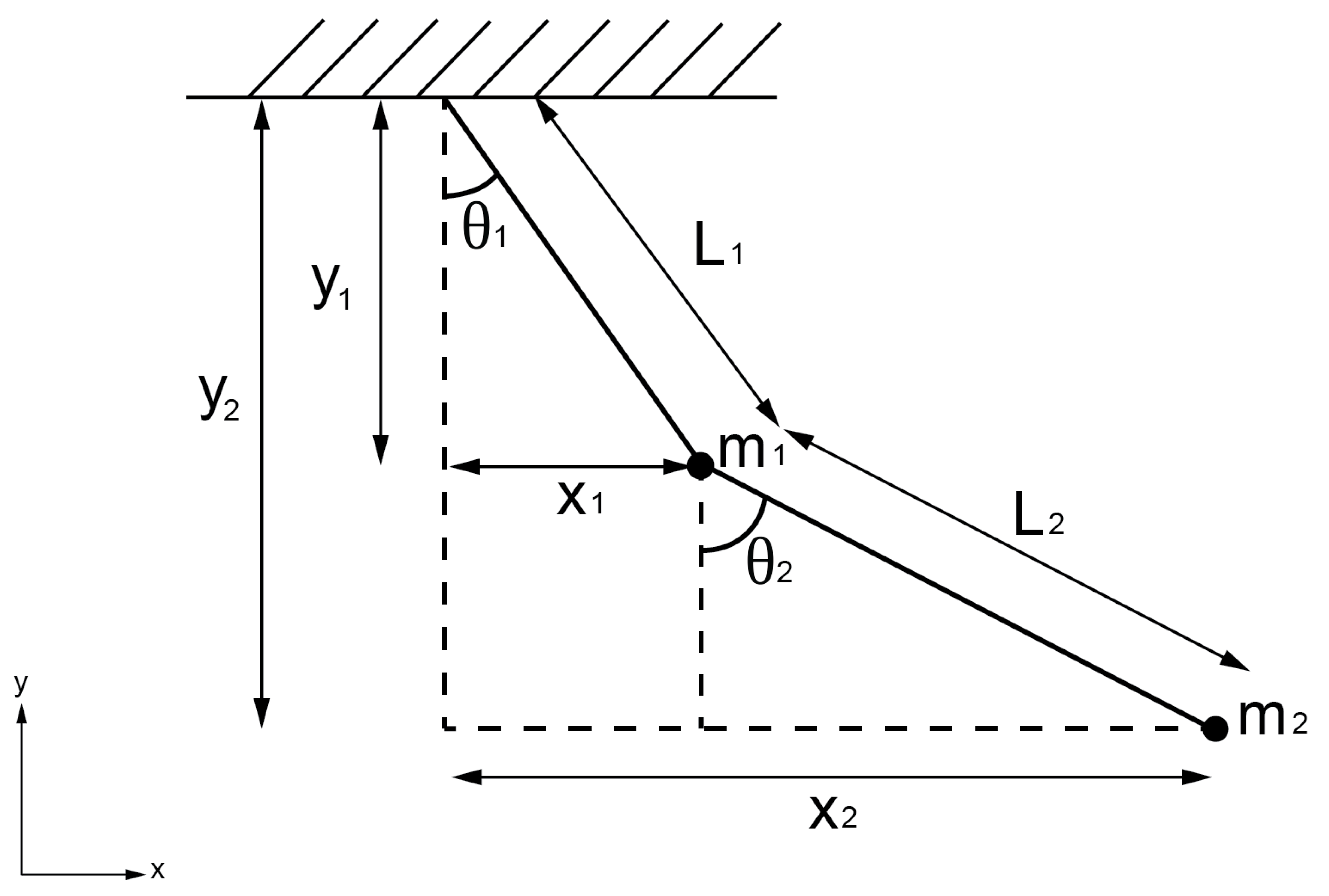
Figure 2. Comparison of (a) execution time and (b) memory usage across different computing environments.

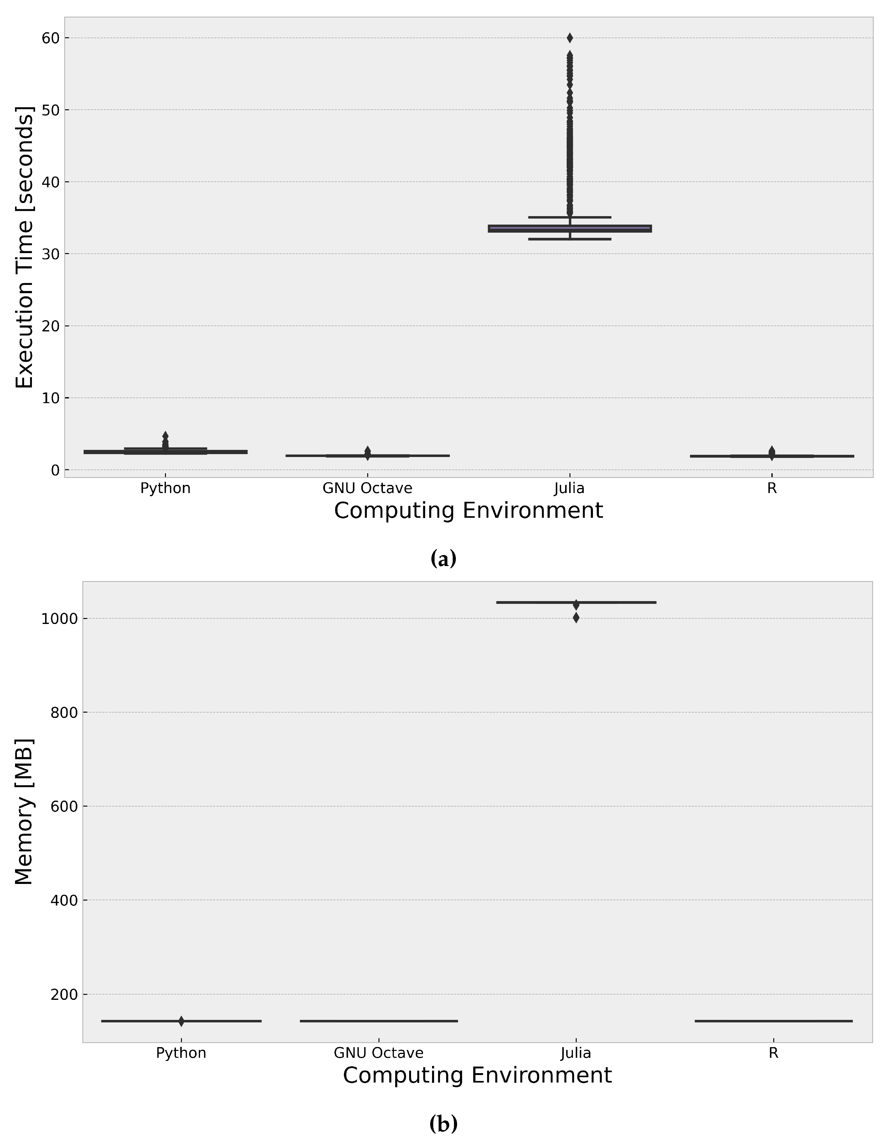
Figure 3. Time series of a double pendulum positions with slightly different initial angular velocities for (a-b) inner and (c - d) outer pendulum.

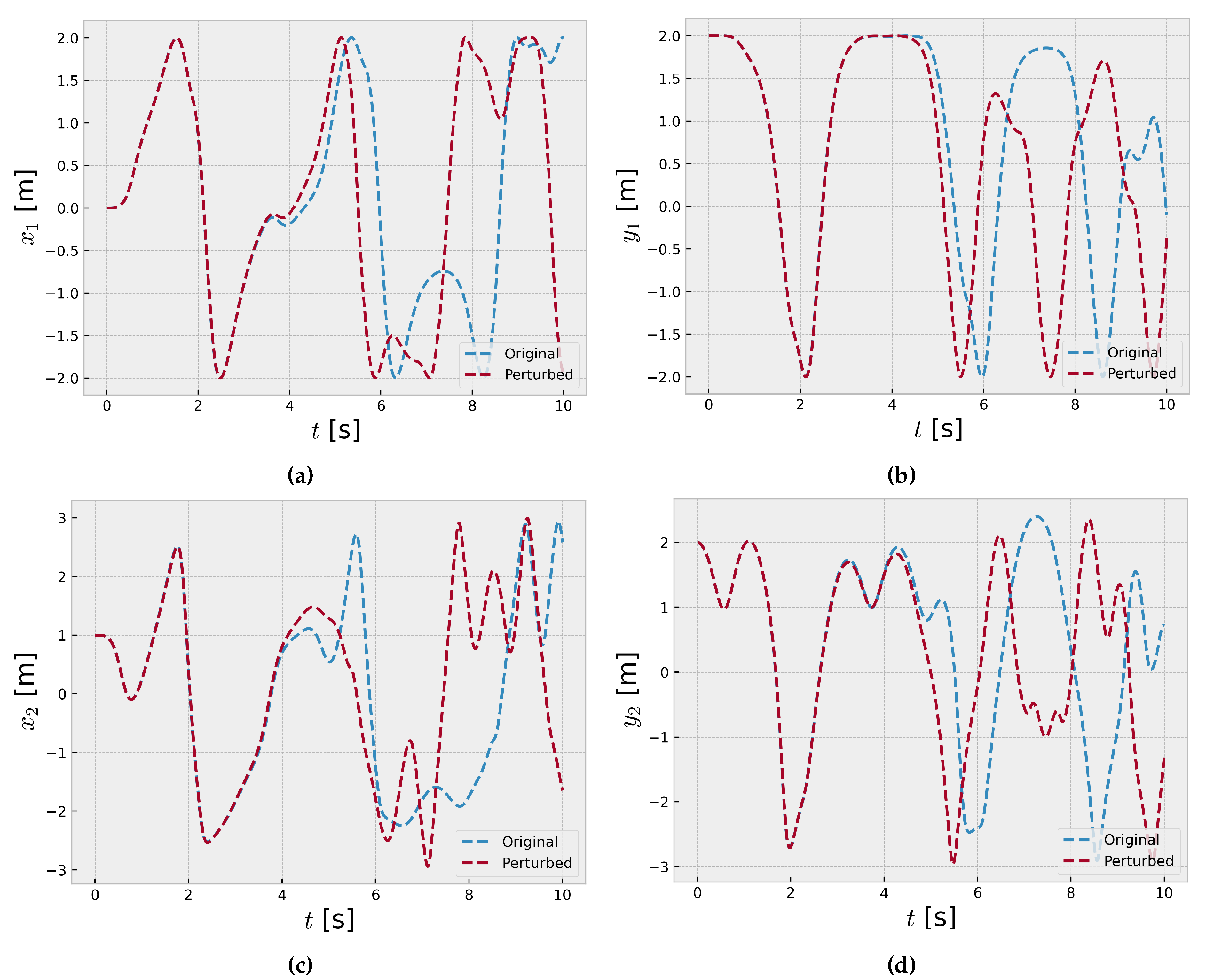
Figure 4. Time series of a double pendulum (a - b) angles and (c - d) angular velocities with slightly different initial angular velocities for (a - c) inner and (b - d) outer pendulum.

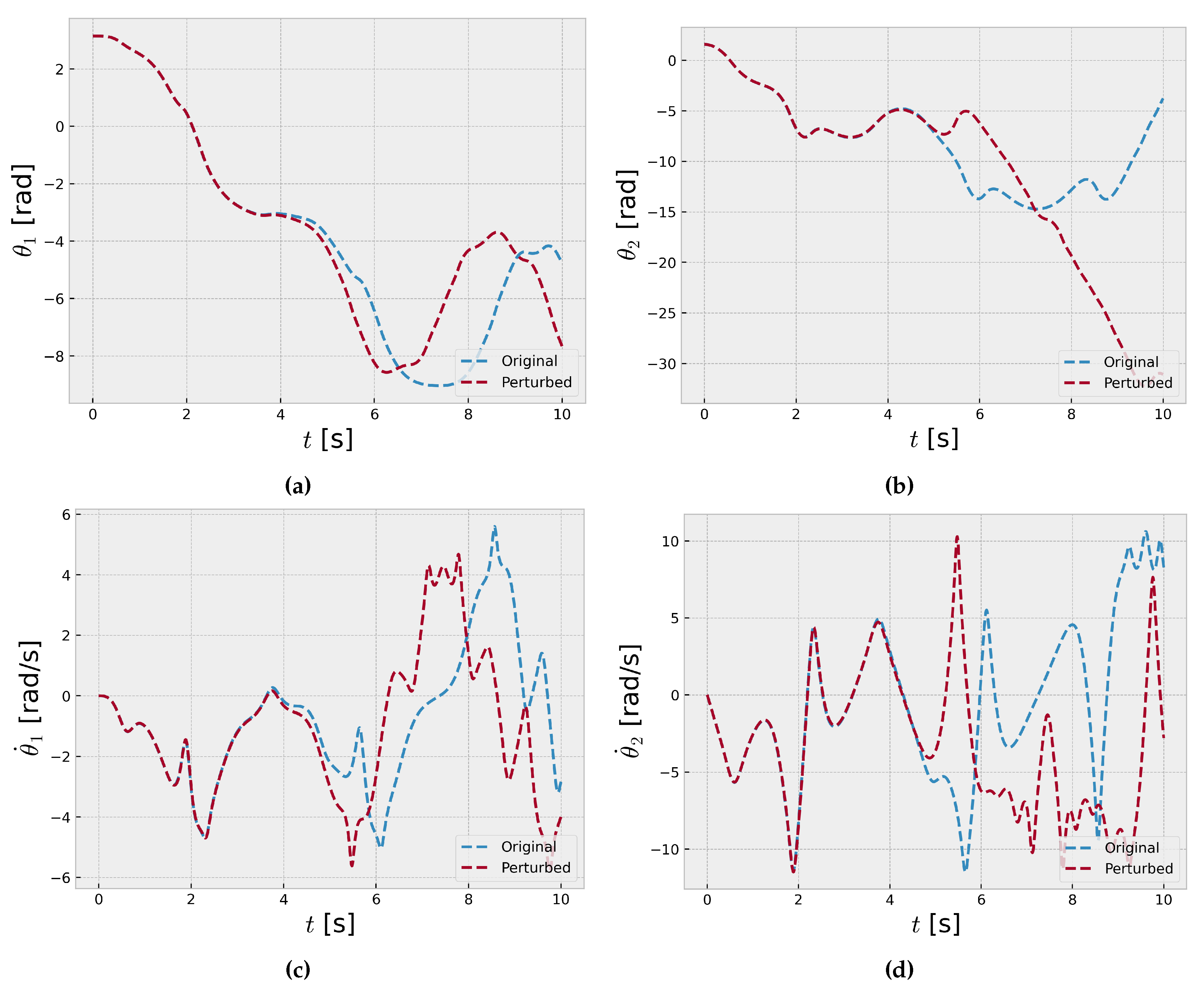
Figure 5. Coupled inner-outer pendulum dynamics. (a - c) Original system. (b - d) System with 0.001 rad/s perturbation to initial angular velocities. (a - b)

x - y

trajectories. (c - d)

θ

vs.

ω

phase space diagrams for inner (blue) and outer (red) pendulums.

Figure 5. Coupled inner-outer pendulum dynamics. (a - c) Original system. (b - d) System with 0.001 rad/s perturbation to initial angular velocities. (a - b)

x - y

trajectories. (c - d)

θ

vs.

ω

phase space diagrams for inner (blue) and outer (red) pendulums.

Disclaimer/Publisher’s Note: The statements, opinions and data contained in all publications are solely those of the individual author(s) and contributor(s) and not of MDPI and/or the editor(s). MDPI and/or the editor(s) disclaim responsibility for any injury to people or property resulting from any ideas, methods, instructions or products referred to in the content.

© 2024 by the authors. Licensee MDPI, Basel, Switzerland. This article is an open access article distributed under the terms and conditions of the Creative Commons Attribution (CC BY) license (http://creativecommons.org/licenses/by/4.0/).

Copyright: This open access article is published under a Creative Commons CC BY 4.0 license, which permit the free download, distribution, and reuse, provided that the author and preprint are cited in any reuse.

MDPI Initiatives

Important Links

Choose an area of interest and we will send you notifications of new preprints at your preferred frequency.

Disclaimer

Reappraising Double Pendulum Dynamics across Multiple Computational Platforms

Abstract

1. Introduction

2. Methods

3. Results and Discussion

4. Conclusions

Acknowledgments

References

MDPI Initiatives

Important Links

Subscribe