
Submitted:
02 May 2024
Posted:
03 May 2024
You are already at the latest version
Abstract
Intrusion Detection Systems play a crucial role in a network. They can detect different network attacks and raise warnings on them. Machine learning-based IDSs are trained on datasets that, due to the context, are inherently large, since they can contain network traffic from different time periods and often include a large number of features. In this paper, we present two contributions: the study of the importance of feature selection when using an IDS dataset, while striking a balance between performance and the number of features; and the study of the feasibility of using a low-capacity device, the Nvidia Jetson Nano, to implement an IDS in a low-capacity network. The results, comparing the GA with other well-known techniques in feature selection and reduction, show that the GA has a higher F1-score of 76%, although the time to find the optimal set of features surpasses other methods; the reduction of the number of features reduces the processing time without a significant impact in f1-score. The Jetson Nano allows the classification of network traffic with an overhead of 10 times in comparison to a traditional server.
Keywords:
feature selection
; genetic algorithms
; machine learning
; HIKARI-2021
1. Introduction
In order to keep network systems operational and secure from Internet attacks, Cybersecurity defensive systems are responsible for producing and processing a sizable amount of data from firewalls, Intrusion Detection Systems (IDS), or Intrusion Prevention Systems (IPS) in the form of network traffic metadata and system logs.
IDS are crucial in the network infrastructure as they provide a security layer that can detect a potential attack going on by analyzing the network traffic in real-time that violates the security policy and compromises its Confidentiality, Integrity, and Availability [1,2].
It began development in the 1980s and since then, it has become a fundamental research and development area within computer security and data protection, and they still growing with enhanced features and improved safety [3].
IDS are divided into three categories according to Jamalipour and Mourali [4]: IDS based on Intrusion Data Sources, IDS based on Detection Techniques, and IDS based on Placement Strategies.
Host-based IDSs (HIDS) and Network-based IDSs (NIDS) are two types of IDS based on intrusion data sources. The HIDS are helpful in identifying assaults on systems including databases, operating systems, and software logs that don’t involve network traffic. In the network environment, NIDS is used to analyze network traffic and find attacks.
Four categories of IDS based on detection techniques using four different techniques can be identified. They can be signature-based IDS, which compares network traffic with a known pattern or signature. Anomaly-based IDS is a different technique that uses pre-defined standards to determine what is malicious or benign based on network protocols. It is quite effective at identifying malicious activity but is unable to identify the specific sort of attack. Similar to anomaly-based IDS, specification-based IDS are based on rules and thresholds specified by experts, but in this case, the rules are implemented based on someone’s competence. Hybrid-based intrusion detection systems (IDS) incorporate both signature-based and anomaly-based approaches, offering the best of "two worlds" in terms of storage cost and computing cost.
There are three types of IDS based on placement strategies: centralized IDS, distributed IDS, and hybrid IDS. To find assaults, centralized IDS examines the data traffic that is going through, either at the root node or a strategic node. Every node in the network will be equipped with a comprehensive IDS, taking advantage of a thorough analysis of each node to prevent attacks from both inside and outside the network. This is known as distributed IDS placement. A central IDS that is better able to analyze huge amounts of data is combined with a variety of lightweight nodes dispersed around the network that have a lower detection ratio but are nonetheless sufficient for the purpose of a hybrid IDS placement.
The ability to distinguish between benign and malicious (attack) packets is crucial when designing a Network Intrusion Detection System (NIDS) based on Machine Learning (ML) algorithms. This success depends heavily on the availability of historical data on attack types and their characteristics.
In the case of the NIDS, which is the current studied topic, there are already various well-known datasets that cover a wide range of attack types, including CICIDS-2017 [5], KDD [6], NSL-KDD [7], UNSW-NB15 [8], and the most recent, HIKARI-2021 [9].
The network traffic-related datasets from the NIDS contain a lot of entries and features. The metadata from a single packet moving across the network can be quite large, and the majority of the datasets described start with 50 features or more; some even have more than 500,000 entries.
The problem and in some cases the benefits of having large datasets is the high number of features. Feature analysis is part of the Exploratory Data Analysis (EDA) step when researchers must understand what is the impact of each feature and decided if it must be used to train the model or if it must be changed in some way, like normalization, or even discard them [10]. Choosing the best features to use to train the model is key for getting the results to address a specific problem. The number and the types of features will make a significant impact in different aspects: the time needed to train and to infer, the results of the model when predicting, and its explainability. Feature selection has many benefits for the models such as the prevention of over-fitting, it prevents noise resistance and it improves predictive performance and some studies show that a lower number of features can increase the detection rate [11].
R. Antunes et al [12] divide the feature selection into 3 types: filter, wrapper, and embedded methods. The filter method is based on the preprocessing of the data which is based on the findings from Exploratory Data Analysis where we use algorithms to rank the features based on statistics such as the correlation, chi-square, and others. The wrapper method consists of using an ML algorithm itself to train a model, and return the most significant features from it, and use them to train a new model with those identified before [13]. The embedded method consists of selecting the features during the training phase without the need to split the dataset into train and test. This reduces the computation time of the training since it optimizes the number of features to use faster than the other two approaches mentioned before.
Genetic algorithms have garnered significant attention from the intrusion detection research community due to their close alignment with the requirements for building efficient intrusion detection systems. The high re-trainability of Genetic Algorithms enhances the adaptability of intrusion detection systems, while their ability to evolve over time through crossover and mutation makes them a suitable choice for dynamic rule generation [14].
Due to the rapidly evolving of Cybersecurity threats, IDS can quickly become outdated as new exploits and attacks emerge. This ongoing challenge require systems that are adaptive and capable of continuous learning. Consequently, Machine Learning (ML) has become essential in this field. ML-based Intrusion Detection Systems have been developed and are showing promising results in classifying network traffic effectively [15,16].
In this research, we studied the feature selection step by reducing the feature dimensionality using a Genetic Algorithm in the HIKARI-2021 dataset. The main goal is to retain only the most relevant and important features, without sacrificing the accuracy of the machine learning model trained on the full dataset. To accomplish this, an XGBoost ML model is deployed, which is known for its ability to handle large datasets and identify complex relationships between features.
The XGBoost algorithm can be described as an ML algorithm that uses the decision-tree-based predictive model through gradient boosting frameworks [17]. This algorithm, designed for speed and efficiency, maximizes memory and hardware efficiency in tree-boosting algorithms and supports deployment across various computing environments [18].
The combination of the Genetic Algorithm and XGBoost model will also be compared to other dimensionality reduction techniques, Principal Component Analysis (PCA), Linear Discriminant Analysis (LDA), and the Chi Squared-test results from a previous study [19].
The end goal of this research is the deployment of the ML-based IDS in an embedded system to behave as an IDS. Embedded systems are creating a huge impact on the way people live nowadays enhancing applications in the areas of health, military, IoT, industry, and automation, among others [20].
For this, a Nvidia Jetson Nano is used as the hardware to support the AI-based IDS running with the subset of features chosen by our Genetic Algorithm and predicting with the trained model XGboost and a comparison will be made regarding the time needed to predict between the jetson nano and the server used to run the Genetic Algorithms.
The paper is organized as follows: the next section presents the Related Work discussing similar approaches from previous research, the Exploratory Data Analysis shows an analysis of the HIKARI-2021 dataset, the Feature Dimensionality Reduction Techniques explain how we design our tests and parameters of the feature selection algorithms used and the Results and Discussion section shows a comparison between the results obtained and the last section concludes our work.
2. Related Work
Different algorithms for supervised learning were already tested in the HIKARI-2021 dataset such as gradient boosting machine (GBM), Light GBM, CatBoost, and XGBoost in the research made by Maya Louk [21], a Multi-layer Perception [22], Graph Neural Networks (GNNs) [23] and other traditional ML algorithms such as KNN, Random Forest and SVM [19]. Although some of them achieve great results and interesting findings, most of the studies mention the importance of further research in the dataset by using different models. Different feature selection techniques and Genetic Algorithms have already proved some value for this case, as in IDS is very common to have datasets with a large number of features.
For the same purpose of this research, building an AI-based ID, Ajeet Rai studied the impact and optimization of Ensemble Methods and Deep Neural Networks by implementing feature selection using Genetic Algorithms, reducing from 122 to 43 features, [24] and their results show that three in a total of four algorithms have better results when using feature selection. Those results were made in a small sub-dataset of the original KDD which probably indicates that by using more data, the results could be even better.
On a different dataset, NSL-KDD, the researchers [25] tested three known algorithms for feature selection - Correlation-based Feature Selection (CFS), Information Gain (IG) and Correlation Attribute Evaluator (CAE) with a Genetic Algorithm - to compare the performance of a Naive Bayes and J48 model. They also concluded that the Genetic Algorithm outperforms the others in the score while reducing the time complexity.
Researchers in [26] used the UNSW-NB15 dataset to compare different dimensionality reduction techniques: the particle swarm optimization (PSO), grey wolf optimizer (GWO), firefly optimization (FFA) and Genetic Algorithm (GA). Their results showed that the PSO achieved better accuracy and precision than the others for the algorithms J48 and SVM. Another interesting finding in this study was that it created new subsets from each subset of all individual algorithms and tested different combinations of features based on joining (inner/out) features. This achieved even better results than using just one algorithm for feature reduction.
Embedded systems are becoming popular in the field of IDS due its their ability to be placed anywhere, the low power consumption, and the cheap cost. Research shows that even an Arduino Uno can behave as an IDS using AI [27]. Another extensive study was made by comparing other low-power embedded systems with different models trained in different conditions proposing a lightweight optimized deep learning IDS [28]. Although these result shows great potential when the model starts to get bigger and the amount of data increase it is necessary for more computational power. Our approach of using the Nvidia Jetson Nano is not so common in the IDS context but it is already used in other cases such as Home intrusions using computer vision and other techniques [29]
3. Materials and Methods
This research uses as materials the most recent IDS dataset - HIKARI 2021 [9] which is publically available. The methods used in this research consist of an Exploratory Data Analysis using statistics algorithms, data preprocessing using Python libraries, and then machine learning algorithms to train a model and then infer data on it.
The system architecture that supports the materials and methods used in this research, Figure 1, consists of five phases: Exploratory Data Analysis where it is studied the dataset (HIKARI) regarding its content - features and data, then Data Preprocessing that applies dimensionality reduction and feature selection that are the different methods studied, then the Model Training using the XGBoost algorithm and the best subset of features chosen before and lastly the deployment of the model to the embedded system.
In the embedded system the same performance evaluation is made as well as in the server that ran the other experiments. This test consists of running the different models trained with different numbers of features and measuring the time. The goal is to keep the classification performance and verify which runs faster and if the embedded system could be a better approach to this use case.
3.1. Exploratory Data Analysis (EDA) to the HIKARI-2021 Dataset
The HIKARI-2021 [9] dataset is currently the most up-to-date, containing encrypted synthetic attacks and benign traffic. The main advantage of this dataset compared to the others is that the network logs are only anonymous in specific logs of benign traffic, the dataset can be reproducible, has ground-through data, and the main characteristic that distinguishes it from the others - having encrypted traffic.
This dataset has a total of 555 278 records, and 88 features, where 2 of them are labels (one binary and other string) where one corresponds to 1 if the traffic is malicious and 0 means benign or background, and another label that classifies the traffic into the different categories: Benign, Background, Probing, Bruteforce, Bruteforce-XML and XMRIGCC-CryptoMiner.
In Table 1 it is possible to see the names of the features as well as their types. Most of them are integers or floats which are related to the traffic analysis and some are strings related to the identification of the source/destiny and label.
One problem of this dataset, which is normal in datasets of IDS, is the fact of being unbalanced. Table 2 shows well how unbalanced the dataset is, having the most quantity of traffic in the benign and background traffic which is normal traffic.
Based on a HIKARI-related study [10] the authors conducted a feature analysis that concluded that some of the features might be removed to accomplish better results. The same approach was followed here, removing the columns: "Unnamed: 0.1", "Unnamed: 0.2", "uid", "originh" and "originp" which are not relevant for a generic classification model but contribute to bias the training step of the classification by learning specific id tags that would otherwise not appear in a real traffic dataset.
3.2. Data Preprocessing
Regarding the data, the preprocessing methods are endless and they must be used according to the data type and the problem we are dealing with. This research, as mentioned previously, addresses the problem of IDS which have a large number of features. Hence techniques related to Dimensionality Reduction and Feature Selection were used.
3.2.1. Dimensionality Reduction
Feature reduction techniques are methods used to reduce the dimensionality of a dataset by selecting or transforming the most important features while retaining as much relevant information as possible.
These techniques are particularly useful in machine learning and data analysis to address issues related to high dimensionality, multicollinearity, and overfitting. The high dimensionality of IDS datasets makes them an excellent use case of these methods since we can get a better understanding of the importance of each feature and we can also reduce the training and inference times of the models used for intrusion detection tasks.
There are two main groups for feature reduction techniques: Feature Extraction and Feature Selection [30].
In Feature Extraction, techniques reduce the dimensionality of the dataset by transforming the original features into a new set of features, that are a mapping of the original ones, while trying to preserve the essential information and patterns present in the data. One disadvantage is that when the original features have an obvious physical meaning, the new features may lose meaning. Methods like Principal Component Analysis (PCA) and Linear Discriminant Analysis (LDA) fall into this category.
PCA reduces the complexity of high-dimensional data by identifying principal components — orthonormal eigenvector and eigenvalue pairs — where data variance is maximized. It projects the data onto these components, focusing on those with the highest eigenvalues, and compressing the data while preserving essential information [31].
LDA projects the n-dimensional dataset into a smaller k-dimensional dataset (k < n), while at the same time maintaining all the relevant class discrimination information [32].
Feature Selection, on the other hand, focuses on selecting a subset of the original features while discarding the rest. The Selected Features are considered the most relevant for the specific task, and irrelevant or redundant features are removed. Chi-squared (Chi-2) and Genetic Algorithms (GA) are both feature selection methods.
Chi-squared is a numerical test that measures the deviation from the expected distribution considering the feature event is independent of the class value [33]. Its use can be as simple as importing the method from the scikit-learn and defining a K number of top features that have more impact on the label.
3.2.2. Genetic Algorithm for Feature Selection
A Genetic Algorithm (GA) is an optimization strategy that operates on a population of potential solutions, often represented as individuals or candidate solutions, and use genetic operators such as selection, crossover, and mutation to evolve and improve the population over generations. This type of algorithm has been around for many years and has proven itself as a a useful approach to finding solutions to real-world complex problems.
It can also be used to perform dimensionality reduction of the dataset. In a Genetic Algorithm approach, the genomes represent a subset of features in the dataset, and the fitness function is used to evaluate the quality of the dimensionality reduction. The fitness function measures the accuracy of machine learning model trained on the reduced dataset, with higher accuracy indicating a better dimensionality reduction.
3.2.3. Genetic Encoding and Initialization
When implementing a GA, the first step is to identify a way to express our solution as a genome. In this case, the genome is a binary one dimensional array with the same length as the number of features in the dataset ( Figure 2), where each bit represents removal or retention of a feature in our dataset (Table 3).
The subsequent step is to randomly initialize a population of arrays with some of the features set to be removed. The number of features removed needs to be chosen beforehand, so that the algorithm will generate arrays with the correct number of features. Each individual is applied to the dataset as a sort of mask, where if a feature is set as ’0’ in the array, it will be removed from the dataset. After going through the entire array, and removing or maintaining features, the resulting dataset is ready to the evaluated.
This population is evaluated through a fitness score. In this case, the score of each individual can be the accuracy of the machine learning model on a new dataset with only the selected features. The model is trained and tested on the new dataset, and the score is stored so it can be later compared to the other individuals.
The algorithm will evaluate the fitness of each individual by testing the corresponding feature subset’s performance using a ML model. Through successive generations, the Genetic Algorithm refines the population, favoring individuals that lead to better model performance. This iterative process mimics the principles of natural selection, allowing the algorithm to converge towards an optimal solution that balances predictive accuracy and feature number for the given dataset and model.
3.2.4. Sparsity Check
Removing features from the dataset, most of the time, results in a loss in accuracy, especially when random features are dropped. This indicates that a genome composed of a lot of features will probably have a better accuracy than a genome with almost no features so the GA will converge on solutions where almost no features are removed, but since we are aiming to reduce the dataset’s dimensions, there must be a mechanism to control the sparsity levels of genome.
To address this issue, a sparsity check function was built to choose the pruning percentage which one wants to apply to the model, as well as to ensure that the generated offspring meet this criteria; if they do not, an algorithm randomly selects values in the mask to modify, in order to meet the sparsity criteria.
3.2.5. Selection Method
Only a few genomes from this initial generation will be chosen to pass on their genes to the next generation. The selection of pairs of individuals (parents) is solely reliant on their fitness score (float values from 0 to 1). Every individual has a chance of becoming a parent with a probability proportional to its fitness. The fitter individuals have a better chance of breeding and passing on their genes to the next generation. The selection method was a memory- optimized version of the roulette wheel approach [34].
Inside the selection function, an individual’s fitness is compared to a randomly generated float value between 0 and 1; if the fitness is high, there is a larger probability that the random number will be less than the fitness, resulting in the individual being chosen as a parent.
3.2.6. Crossover and Mutation
A Genetic Algorithm’s most important phase is crossover. A crossover point is picked at random from within the genetic code, then the offspring will randomly inherit one side of the crossover point from each parent. When a new generation of offspring is born, some of their genes may be susceptible to a low-probability mutation. This means that some of the bits in the genetic code can be switched around. Mutations are an important step of the GA because it guarantees diversity in the population and prevents premature convergence. Individuals with a high fitness score would soon dominate the population in the absence of mutations, limiting the GA to a local optimum and hindering the GA’s ability to produce superior offspring.
3.3. Model Training
Our model was based on the XGBoost Classifier library and training was done with the SciKit-Learn Python API for XGBoost using all parameters set to default [35].
A crucial way to be confident when saying a model is ready to be used and fits the expectations of the job needed is by evaluating the model. Different metrics can be used, each problem will require its own metrics regarding speed, performance, results, outcomes, and others. For this specific topic and because the focus was the performance of classification it was decided to use the most popular metrics in IDS: accuracy and f1 score.
Accuracy is calculated by dividing the number of correctly identified predictions, true positives (TP) and true negatives (TN), by the total number of predictions (TP+FN+TN+FP) which means that by having a high accuracy the algorithm can be more trusted to classify the traffic but in IDS field accuracy is not the most important because of the existent datasets are imbalanced and the model can label everything as “benign” and achieve high accuracy due the fact the label with the highest frequency is “benign”, balanced accuracy is a better option for this cases.
Precision is calculated by dividing the number of correctly identified malicious predictions, true positives (TP), by the total number of predictions that the algorithm classified as malicious, true positives (TP) + false positive (FP), which means that high precision is valuable to say that we can correctly identify the malicious traffic with a low percentage of false positives.
Recall, also known as Sensitivity or true positive (TP) rate, is a metric that focuses on the ability of a model to correctly identify all positive instances in the dataset. It is calculated by dividing the true positives (TP) by the sum of true positives (TP) and false negatives (FN). In the IDS context recall is a crucial metric since it represents the ability of a model to catch as much malicious traffic as possible. High recall means that the model is able to identify the majority of true threats, however it may lead to more false positives (FP).
The F1 score is a metric that combines both precision and recall providing a balanced measure of a model’s performance. It is useful when it’s wanted to find a balance between precision and recall, ensuring that false positives and false negatives are both minimized. F1 score is the metric that is more trustworthy in IDS studies because the higher it is it ensures that the model not only catches malign traffic but also minimizes false positives.
3.4. Model Inferencing and IDS
Regarding the inference, the idea of building a fully working IDS using AI the different parts are combined into a single system. For that, all of the previous work is now stored in one file - a ".pkl" file containing the model trained. An existing traditional dataset is used as a packet sniffer - ciclfowmeter which is publicly available and for that research, it is used to capture network traffic that is loaded into our model by selecting the features needed for our prediction.
All of these pieces fit into an embedded system - Nvidia Jetson Nano - running a Linux Ubuntu distribution being able to run both cicflowmeter and our model for real-time predictions.
4. Results and Discussion
In this final chapter, we dive into a comparative analysis of dimensionality reduction techniques applied to our dataset in conjunction with the XGBoost model. Specifically, we explore the impact of Feature Reduction using Linear Discriminant Analysis (LDA) and Principal Component Analysis (PCA), as well as Feature Selection through with Chi-squared (Chi-2) and the Genetic Algorithm.
Our goal is to understand the effectiveness of each technique in reducing the dimensions of the HIKARI Dataset while striking a balance with the XGBoost model’s performance.
The server used was a single machine with a dual Intel(R) Xeon(R) CPU E5-2690 v2 @ 3.00GHz 10 core CPU, with 120 GB of RAM with no powerful background apps running simultaneously.
The embedded system, NVIDIA Jetson Nano Developer Kit, is described by NVIDIA as a small, powerful computer designed to run different Neural Networks in parallel for different use cases related to computer vision, speech processing robotics, and others [36]. Nvidia Jetson Nano has a Quad-core ARM A57 @ 1.43 GHz CPU, 128-core Maxwell GPU, and 4 GB LPDDR4 as memory.
4.1. Dimensionality Reduction
As previously mentioned, the two dimensionality reduction techniques utilized were PCA and LDA. With PCA, it was possible to choose between 70 to 1 features. But with LDA it was limited to a maximum of 5 feature dimensions (Table 4).
LDA is a supervised method that aims to find the directions (linear discriminants) that maximize the separation between different classes. The number of linear discriminants is at most c-1, where c is the number of classes. This is because LDA projects data points onto a lower-dimensional space with the goal of maximizing class separability, and the maximum number of discriminative directions is determined by the number of classes [37].
On the other hand, PCA is an unsupervised method that does not take into account class labels. It finds the directions (principal components) that maximize the variance of the data. Therefore, PCA can generate as many principal components as the original dimension of the feature space or the number of samples, whichever is smaller.
Regarding LDA’s effectiveness, from the experimental results, we can see that it achieved lower Accuracy and a lower F1-Score for the same dimensions as PCA. This shows that PCA can strike a better balance between feature dimension and performance.
On both approaches, there is a noticeable decrease in training time as the feature dimension also is reduced, but there isn’t a difference on the inference times on the Test Set, this is due to the high computational power of the Computer used, where the number of data on the Test set is so small that it doesn’t make too much of an impact.

Table 5.
PCA.
| Feature Dimensions | Train time(s) | Test time(s) | Accuracy (%) | F1-Score Weighted (%) |
|---|---|---|---|---|
| 70 | 217.12 | 0.073 | 76.53 | 75.23 |
| 60 | 210.09 | 0.073 | 76.43 | 75.13 |
| 50 | 192.97 | 0.068 | 76.32 | 74.98 |
| 40 | 120.18 | 0.073 | 75.54 | 74.20 |
| 30 | 116.52 | 0.068 | 75.25 | 73.88 |
| 20 | 111.14 | 0.064 | 74.22 | 72.66 |
| 10 | 94.85 | 0.066 | 73.71 | 71.93 |
| 5 | 83.03 | 0.063 | 73.11 | 71.00 |
| 4 | 77.33 | 0.072 | 72.43 | 70.17 |
| 3 | 77.98 | 0.071 | 71.88 | 69.49 |
| 2 | 60.25 | 0.073 | 71.45 | 69.54 |
| 1 | 46.99 | 0.071 | 69.79 | 65.75 |
4.2. Feature Selection
In regards to the Feature Selection techniques, we can see that both Chi-2 and the GA achieved better results than the Feature Reduction of LDA, both Chi-2 ( Table 6) and the GA (Table 7) maintained a higher Accuracy and F1-Score as the feature dimensions lowered. The GA was the one with the better results, it achieved 73.59% F1-Score with only a dimension of 3, beating the PCA and the Chi-2.
The lower results of the Chi-2 compared to the GA can be explained by its approach to feature selection, since It relies on statistical measures to identify the relationship between each feature and the target variable. However, it may not explore the entire feature space comprehensively, and its effectiveness can be limited if the relationship between features. The GA, on the other hand, performs a more exhaustive search of feature combinations through its evolutionary process, making it more likely to discover relevant feature interactions and dependencies.
One of the main drawbacks of the GA is its runtime, as in the total time that the Genetic Algorithm took to go through the various possible candidates in each generation. In Table 7, we can see that it takes a considerable time to find the optimal solution for the different feature dimensions that are selected, this time decreases as the number of dimensions also become smaller but its an important thing to consider, since the other approaches to reduce the dimensions are almost instantaneous.
With these two methods, we can see which features are chosen as the most impactful to the accuracy of the model. On PCA and LDA this was not possible since the features were transformed. In Table 8 and Table 9 the five most important features are shown.
When comparing the results of all the techniques used, we can visualize in Figure 3 that the GA emerged as the most effective approach in maintaining optimal performance even as the number of features was decreased. In contrast, the Chi-2 approach demonstrated a poorer performance when compared to its counterparts.
4.3. Performance Evaluation between the Jetson Nano and the Server
One of the goals of this paper contributions is to assess the feasibility of using an embedded system to implement the IDS functionality. With that in mind, we evaluate all the different models, trained in the Server machine, with the same reference test set in the Jetson device and compare the time needed to infer the complete test set. The results in Table 10 show that the Nvidia Jetson takes 10 times more than the Server to classify the traffic in the test set - about 111,000 entries.
From the results table, it is noticed that although Chi Square is the algorithm that has a higher f1 score, it is also the one that takes more time, both in the Jetson and in the server, to predict the test set. Another relevant aspect is that LDA takes more time to predict the complete test set when configured to use one component than when using five components.
The results can be graphically explained in Figure 4 where the xx axis identifies the number of features considered and the yy axis (which is in log scale) represents the time used in seconds for running the inference on the test set. We can observe that the time needed to infer in the Jetson Nano is 10 times larger than the time needed by the server. It is also visible, both for the server and for the Jetson, that the time taken for the inference increases with the number of features, which is explainable by the complexity of having more features to process.
The Figure 5, also with the xx axis representing the number of features and the yy axis representing the inference time in seconds in log scale, represents the time of the 4 models on the Jetson device. It is easily noticed that the increase on the number of features also increases the time to infer. The exception is the LDA algorithm, where running one component is slower than running with five components.
5. Conclusions
In this work, we study the importance of feature selection when using an IDS dataset. First, an exploratory data analysis was done in the HIKARI-2021 dataset to characterise the features. In order to reduce the model complexity, we propose to reduce the number of features considered, with the goal of achieving the same performance metrics (f1 score) but with a faster time to run the model.
We applied four different algorithms for feature selection on the HIKARI-2021 dataset and performed an evaluation on the performance metrics and running time.
Our study showed that the Genetic Algorithm outperformed the most traditional algorithms such as PCA, LDA or chi-square test. Although the GA presents better results regarding the F1-score, it needs more time than the others to select the number of features more relevant.
We also studied the use of an embedded system, the Nvidia Jetson Nano, to implement the IDS functionality as an edge device. To evaluate this system, a comparison was made between this device and a typical server, showing that the Jetson can behave as an IDS but it takes 10 factor more time than the Server for inferencing a data set.
Author Contributions
Conceptualization, J.S., R.F and N.L.; methodology, J.S., R.F and N.L.; investigation, J.S., R.F and N.L.; writing, J.S., R.F and N.L.; supervision, N.L. All authors have read and agreed to the published version of the manuscript.
Institutional Review Board Statement
Not applicable.
Informed Consent Statement
Not applicable.
Data Availability Statement
Publicly available datasets were analyzed in this study. This data can be found at https://zenodo.org/record/5199540##.ZHcn2nbMJD8.
Conflicts of Interest
The authors declare no conflict of interest. The funders had no role in the design of the study; in the collection, analyses, or interpretation of data; in the writing of the manuscript; or in the decision to publish the results.
References
- Vasilomanolakis, E.; Karuppayah, S.; Mühlhäuser, M.; Fischer, M. Taxonomy and Survey of Collaborative Intrusion Detection. ACM Computing Surveys 2015, 47. [Google Scholar] [CrossRef]
- Denning, D. An Intrusion-Detection Model. IEEE Transactions on Software Engineering 1987, SE-13, 222–232. [Google Scholar] [CrossRef]
- Yost, J.R. The March of IDES: Early History of Intrusion-Detection Expert Systems. IEEE Annals of the History of Computing 2016, 38, 42–54. [Google Scholar] [CrossRef]
- Jamalipour, A.; Murali, S. A Taxonomy of Machine-Learning-Based Intrusion Detection Systems for the Internet of Things: A Survey. IEEE Internet of Things Journal 2022, 9, 9444–9466. [Google Scholar] [CrossRef]
- Sharafaldin, I.; Lashkari, A.H.; Ghorbani, A.A. Toward Generating a New Intrusion Detection Dataset and Intrusion Traffic Characterization. International Conference on Information Systems Security and Privacy, 2018.
- KDD Cup 1999 Data.
- Tavallaee, M.; Bagheri, E.; Lu, W.; Ghorbani, A.A. A detailed analysis of the KDD CUP 99 data set. 2009 IEEE Symposium on Computational Intelligence for Security and Defense Applications, 2009, pp. 1–6. [CrossRef]
- Moustafa, N.; Slay, J. UNSW-NB15: a comprehensive data set for network intrusion detection systems (UNSW-NB15 network data set). 2015 Military Communications and Information Systems Conference (MilCIS), 2015, pp. 1–6. [CrossRef]
- Ferriyan, A.; Thamrin, A.H.; Takeda, K.; Murai, J. Generating Network Intrusion Detection Dataset Based on Real and Encrypted Synthetic Attack Traffic. Applied Sciences 2021, 11. [Google Scholar] [CrossRef]
- Fernandes, R.; Silva, J.; Ribeiro, O.; Portela, I.; Lopes, N. The impact of identifiable features in ML Classification algorithms with the HIKARI-2021 Dataset. 2023 11th International Symposium on Digital Forensics and Security (ISDFS), 2023, pp. 1–5. [CrossRef]
- Almomani, O. A Feature Selection Model for Network Intrusion Detection System Based on PSO, GWO, FFA and GA Algorithms. Symmetry 2020, 12. [Google Scholar] [CrossRef]
- Rita Antunes, A.; Silva, J.P.; Cristina Braga, A.; Gonçalves, J. Feature Selection Optimization for Heart Rate Variability. 2023 11th International Symposium on Digital Forensics and Security (ISDFS), 2023, pp. 1–6. [CrossRef]
- Hasan, M.; Nasser, M.; Ahmad, S.; Molla, K. Feature Selection for Intrusion Detection Using Random Forest. Journal of Information Security 2016, 7, 129–140. [Google Scholar] [CrossRef]
- Majeed, P.G.; Kumar, S. Genetic algorithms in intrusion detection systems: A survey. International Journal of Innovation and Applied Studies 2014, 5, 233. [Google Scholar]
- Halimaa A., A.; Sundarakantham, K. Machine Learning Based Intrusion Detection System. 2019 3rd International Conference on Trends in Electronics and Informatics (ICOEI), 2019, pp. 916–920. [CrossRef]
- Ahmad, Z.; Shahid Khan, A.; Shiang, C.; Ahmad, F. Network intrusion detection system: A systematic study of machine learning and deep learning approaches. Transactions on Emerging Telecommunications Technologies 2021, 32. [Google Scholar] [CrossRef]
- Chen, Z.; Jiang, F.; Cheng, Y.; Gu, X.; Liu, W.; Peng, J. XGBoost Classifier for DDoS Attack Detection and Analysis in SDN-Based Cloud. 2018 IEEE International Conference on Big Data and Smart Computing (BigComp), 2018, pp. 251–256. [CrossRef]
- Dhaliwal, S.S.; Nahid, A.A.; Abbas, R. Effective Intrusion Detection System Using XGBoost. Information 2018, 9. [Google Scholar] [CrossRef]
- Fernandes, R.; Lopes, N. Network Intrusion Detection Packet Classification with the HIKARI-2021 Dataset: a study on ML Algorithms. 2022 10th International Symposium on Digital Forensics and Security (ISDFS), 2022, pp. 1–5. [CrossRef]
- Ajani, T.S.; Imoize, A.L.; Atayero, A.A. An Overview of Machine Learning within Embedded and Mobile Devices–Optimizations and Applications. Sensors 2021, 21. [Google Scholar] [CrossRef] [PubMed]
- Louk, M.H.L.; Tama, B.A. Dual-IDS: A bagging-based gradient boosting decision tree model for network anomaly intrusion detection system. Expert Systems with Applications 2023, 213, 119030. [Google Scholar] [CrossRef]
- Kabla, A.H.H.; Thamrin, A.H.; Anbar, M.; Manickam, S.; Karuppayah, S. PeerAmbush: Multi-Layer Perceptron to Detect Peer-to-Peer Botnet. Symmetry 2022, 14. [Google Scholar] [CrossRef]
- Wang, L.; Cheng, Z.; Lv, Q.; Wang, Y.; Zhang, S.; Huang, W. ACG: Attack Classification on Encrypted Network Traffic using Graph Convolution Attention Networks. 2023 26th International Conference on Computer Supported Cooperative Work in Design (CSCWD), 2023, pp. 47–52. [CrossRef]
- Rai, A. Optimizing a New Intrusion Detection System Using Ensemble Methods and Deep Neural Network. 2020 4th International Conference on Trends in Electronics and Informatics (ICOEI)(48184), 2020, pp. 527–532. [CrossRef]
- Desale, K.S.; Ade, R. Genetic algorithm based feature selection approach for effective intrusion detection system. 2015 International Conference on Computer Communication and Informatics (ICCCI), 2015, pp. 1–6. [CrossRef]
- Almomani, O. A Feature Selection Model for Network Intrusion Detection System Based on PSO, GWO, FFA and GA Algorithms. Symmetry 2020, 12. [Google Scholar] [CrossRef]
- de Almeida Florencio, F.; Moreno, E.D.; Teixeira Macedo, H.; de Britto Salgueiro, R.J.P.; Barreto do Nascimento, F.; Oliveira Santos, F.A. Intrusion Detection via MLP Neural Network Using an Arduino Embedded System. 2018 VIII Brazilian Symposium on Computing Systems Engineering (SBESC), 2018, pp. 190–195. [CrossRef]
- Idrissi, I.; Azizi, M.M.; Moussaoui, O. A Lightweight Optimized Deep Learning-based Host-Intrusion Detection System Deployed on the Edge for IoT. International Journal of Computing and Digital Systems 2021, 11. [Google Scholar] [CrossRef]
- Sahlan, F.; Feizal, F.Z.; Mansor, H. Home Intruder Detection System using Machine Learning and IoT. International Journal on Perceptive and Cognitive Computing 2022, 8, 56–60. [Google Scholar]
- Jia, W.; Sun, M.; Lian, J.; Hou, S. Feature dimensionality reduction: a review. Complex & Intelligent Systems 2022, 8, 2663–2693. [Google Scholar]
- Heba, F.E.; Darwish, A.; Hassanien, A.E.; Abraham, A. Principle components analysis and Support Vector Machine based Intrusion Detection System. 2010 10th International Conference on Intelligent Systems Design and Applications, 2010, pp. 363–367. [CrossRef]
- Subba, B.; Biswas, S.; Karmakar, S. Intrusion Detection Systems using Linear Discriminant Analysis and Logistic Regression. 2015 Annual IEEE India Conference (INDICON), 2015, pp. 1–6. [CrossRef]
- Sumaiya Thaseen, I.; Aswani Kumar, C. Intrusion detection model using fusion of chi-square feature selection and multi class SVM. Journal of King Saud University - Computer and Information Sciences 2017, 29, 462–472. [Google Scholar] [CrossRef]
- Jebari, K.; Madiafi, M. Selection methods for genetic algorithms. International Journal of Emerging Sciences 2013, 3, 333–344. [Google Scholar]
- XGBoost. XGBoost Classifier Parameters. https://xgboost.readthedocs.io/en/stable/parameter.html. Accessed: 2024-01-02.
- NVIDIA. Jetson Nano Developer Kit. https://developer.nvidia.com/embedded/jetson-nano-developer-kit. Accessed: 2023-12-21.
- Tharwat, A.; Gaber, T.; Ibrahim, A.; Hassanien, A.E. Linear discriminant analysis: A detailed tutorial. AI communications 2017, 30, 169–190. [Google Scholar] [CrossRef]
Figure 1.
System Architecture
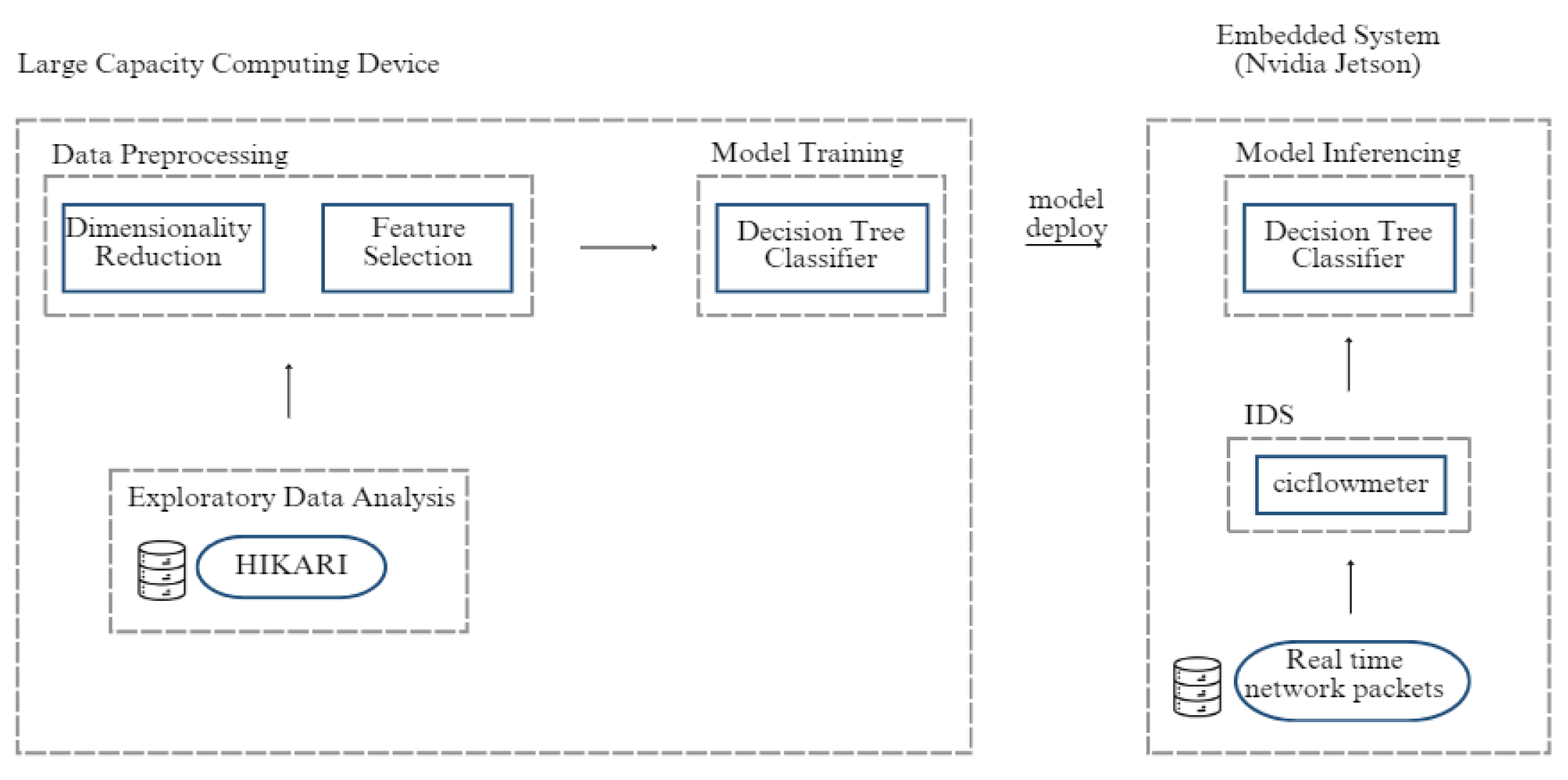
Figure 2.
Genetic encoding of Dataset.
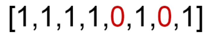
Figure 3.
Feature number vs F1-score (X Axis is in log scale).
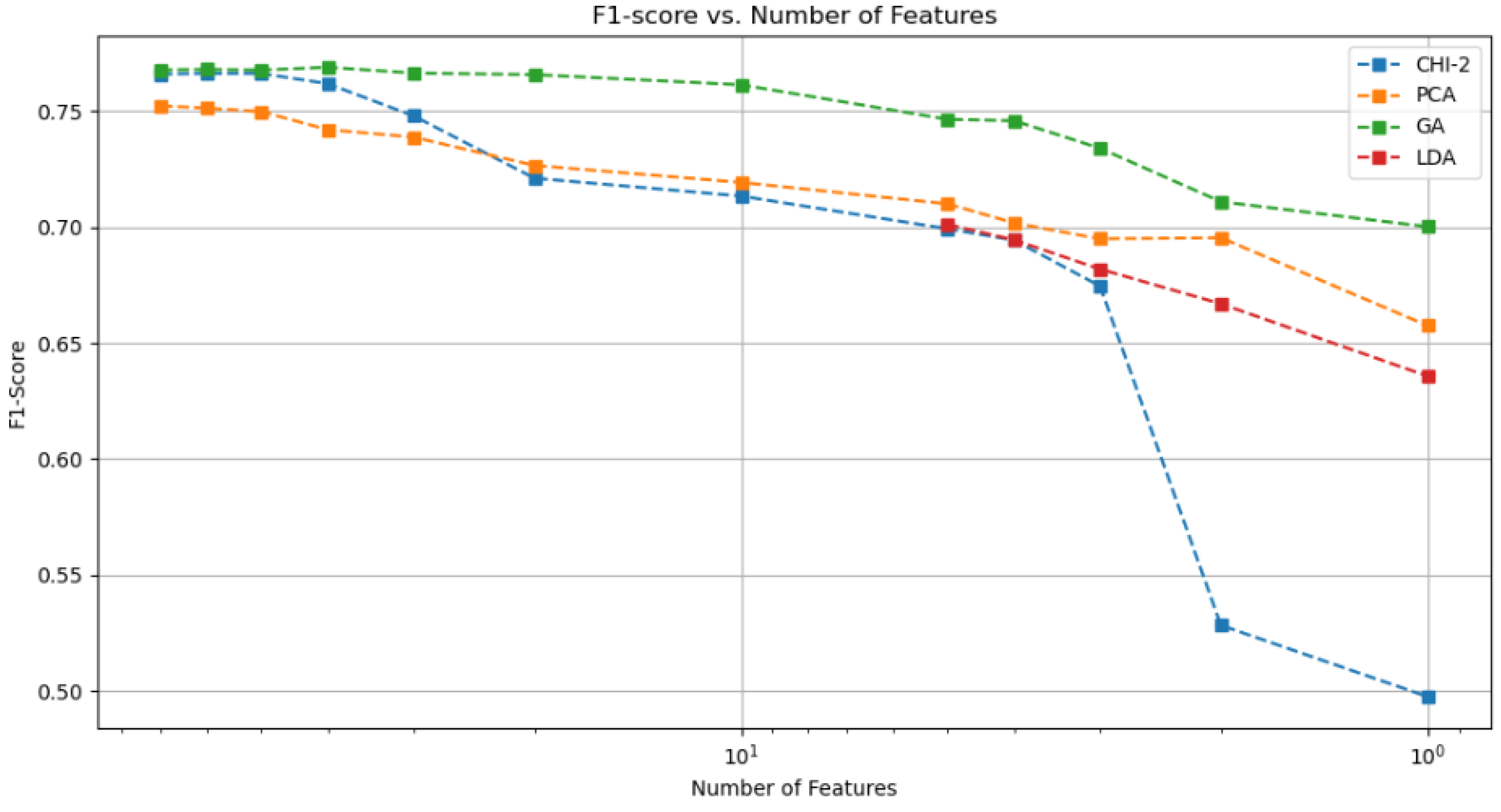
Figure 4.
Time vs number of features (YY axis is in log scale).
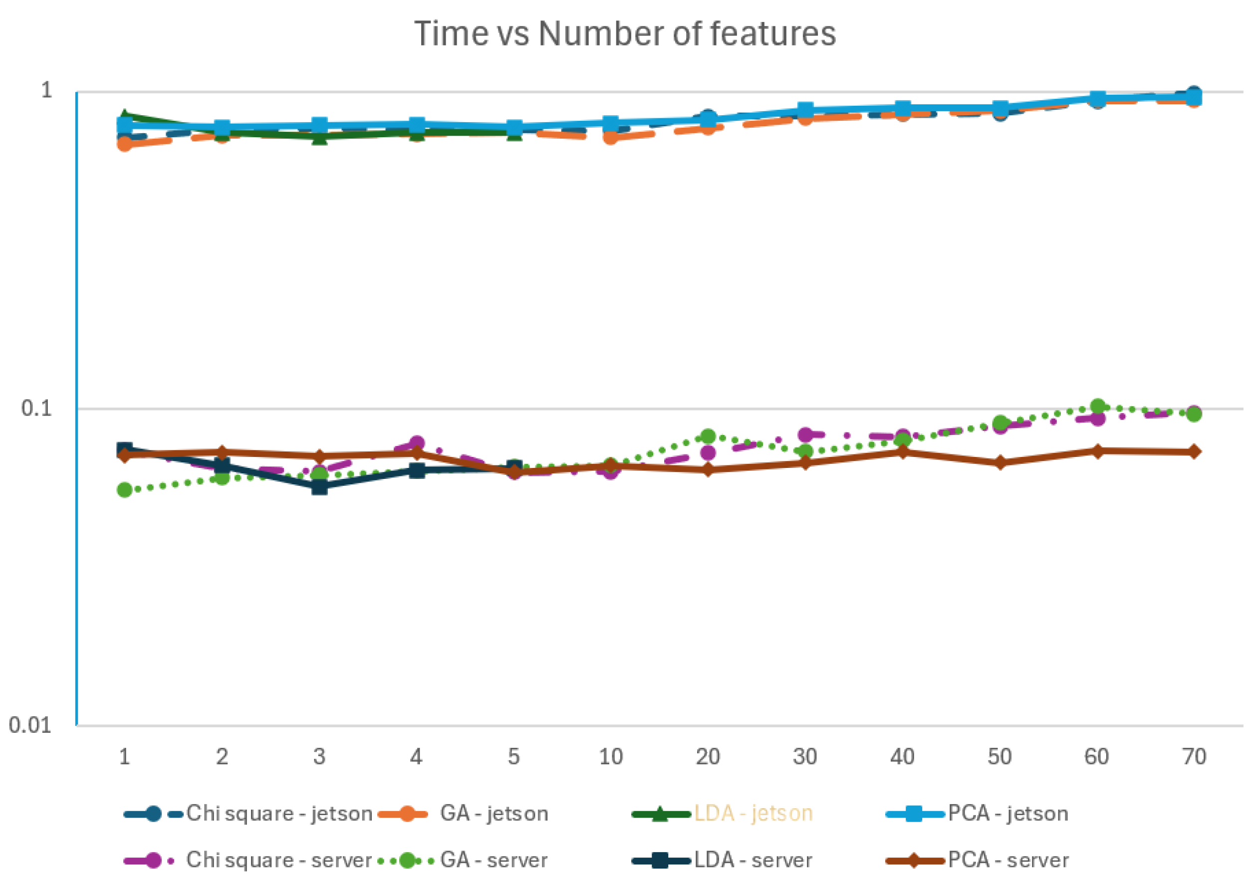
Figure 5.
Time vs number of features in the Jetson (yy axis is in log scale).
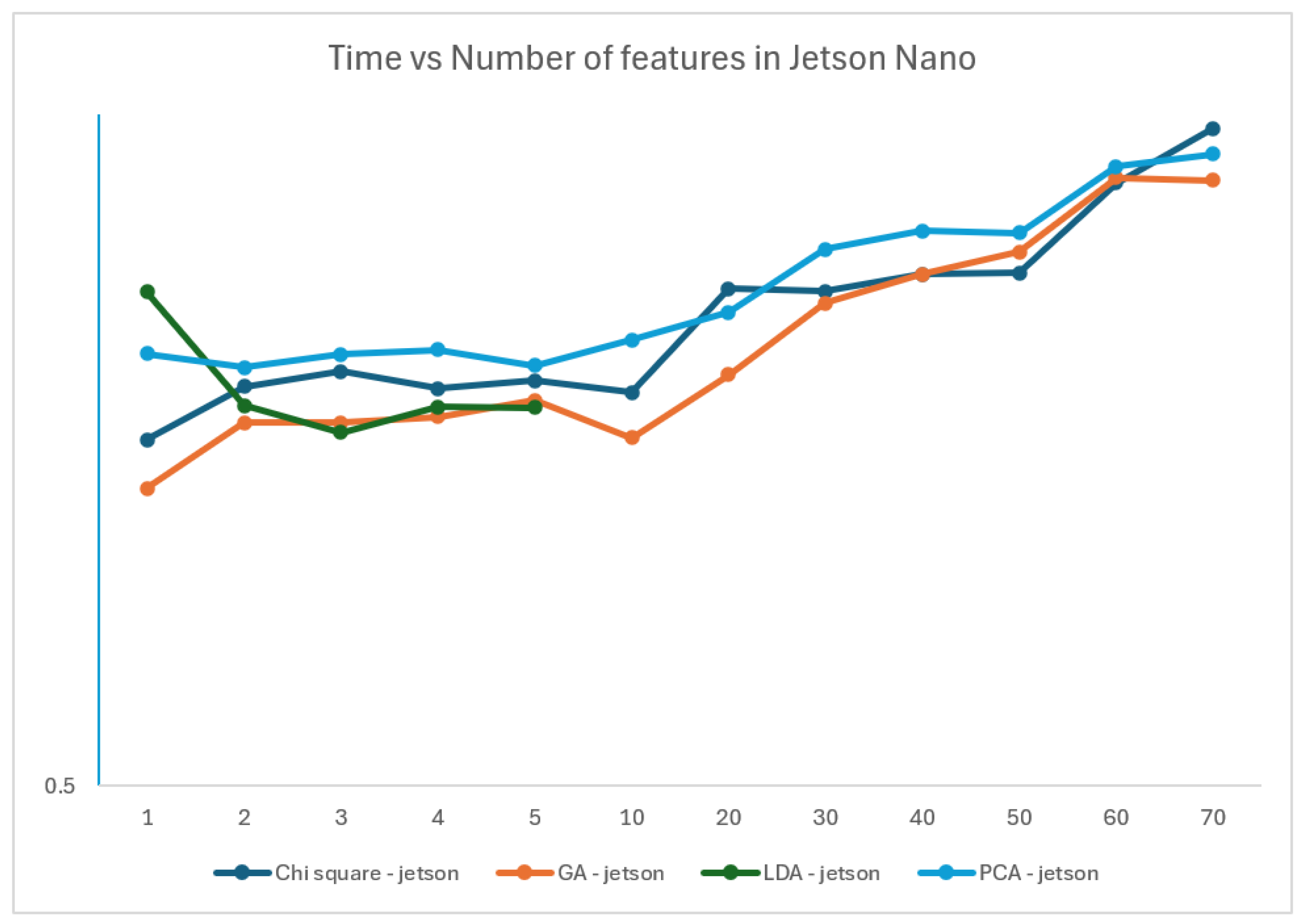
Table 1.
Features names and Types for HIKARI-2021 dataset.
| Feature name |
Feature type |
Feature name |
Feature type |
Feature name |
Feature type |
|||
| 1 | Unnamed: 0.1 | int64 | 31 | flow_CWR_flag_count | int64 | 61 | flow_iat.avg | float64 |
| 2 | Unnamed: 0 | int64 | 32 | flow_ECE_flag_count | int64 | 62 | flow_iat.std | float64 |
| 3 | uid | string | 33 | fwd_pkts_payload.min | float64 | 63 | payload_bytes_per_second | float64 |
| 4 | originh | string | 34 | fwd_pkts_payload.max | float64 | 64 | fwd_subflow_pkts | float64 |
| 5 | originp | int64 | 35 | fwd_pkts_payload.tot | float64 | 65 | bwd_subflow_pkts | float64 |
| 6 | responh | string | 36 | fwd_pkts_payload.avg | float64 | 66 | fwd_subflow_bytes | float64 |
| 7 | responp | int64 | 37 | fwd_pkts_payload.std | float64 | 67 | bwd_subflow_bytes | float64 |
| 8 | flow_duration | float64 | 38 | bwd_pkts_payload.min | float64 | 68 | fwd_bulk_bytes | float64 |
| 9 | fwd_pkts_tot | int64 | 39 | bwd_pkts_payload.max | float64 | 69 | bwd_bulk_bytes | float64 |
| 10 | bwd_pkts_tot | int64 | 40 | bwd_pkts_payload.tot | float64 | 70 | fwd_bulk_packets | float64 |
| 11 | fwd_data_pkts_tot | int64 | 41 | bwd_pkts_payload.avg | float64 | 71 | bwd_bulk_packets | float64 |
| 12 | bwd_data_pkts_tot | int64 | 42 | bwd_pkts_payload.std | float64 | 72 | fwd_bulk_rate | float64 |
| 13 | fwd_pkts_per_sec | float64 | 43 | flow_pkts_payload.min | float64 | 73 | bwd_bulk_rate | float64 |
| 14 | bwd_pkts_per_sec | float64 | 44 | flow_pkts_payload.max | float64 | 74 | active.min | float64 |
| 15 | flow_pkts_per_sec | float64 | 45 | flow_pkts_payload.tot | float64 | 75 | active.max | float64 |
| 16 | down_up_ratio | float64 | 46 | flow_pkts_payload.avg | float64 | 76 | active.tot | float64 |
| 17 | fwd_header_size_tot | int64 | 47 | flow_pkts_payload.std | float64 | 77 | active.avg | float64 |
| 18 | fwd_header_size_min | int64 | 48 | fwd_iat.min | float64 | 78 | active.std | float64 |
| 19 | fwd_header_size_max | int64 | 49 | fwd_iat.max | float64 | 79 | idle.min | float64 |
| 20 | bwd_header_size_tot | int64 | 50 | fwd_iat.tot | float64 | 80 | idle.max | float64 |
| 21 | bwd_header_size_min | int64 | 51 | fwd_iat.avg | float64 | 81 | idle.tot | float64 |
| 22 | bwd_header_size_max | int64 | 52 | fwd_iat.std | float64 | 82 | idle.avg | float64 |
| 23 | flow_FIN_flag_count | int64 | 53 | bwd_iat.min | float64 | 83 | idle.std | float64 |
| 24 | flow_SYN_flag_count | int64 | 54 | bwd_iat.max | float64 | 84 | fwd_init_window_size | int64 |
| 25 | flow_RST_flag_count | int64 | 55 | bwd_iat.tot | float64 | 85 | bwd_init_window_size | int64 |
| 26 | fwd_PSH_flag_count | int64 | 56 | bwd_iat.avg | float64 | 86 | fwd_last_window_size | int64 |
| 27 | bwd_PSH_flag_count | int64 | 57 | bwd_iat.std | float64 | 87 | traffic_category | string |
| 28 | flow_ACK_flag_count | int64 | 58 | flow_iat.min | float64 | 88 | Label | int64 |
| 29 | fwd_URG_flag_count | int64 | 59 | flow_iat.max | float64 | |||
| 30 | bwd_URG_flag_count | int64 | 60 | flow_iat.tot | float64 |
Table 2.
Distribution of the HIKARI-2021 dataset per label.
| Traffic Category | Frequency |
| Benign | 347431 |
| Background | 170151 |
| Probing | 23388 |
| Bruteforce | 5884 |
| Bruteforce-XML | 5145 |
| XMRIGCC CryptoMiner | 3279 |
Table 3.
Features in Array.
| Features | Removed |
|---|---|
| Feature 1 | No |
| Feature 2 | No |
| Feature 3 | No |
| Feature 4 | No |
| Feature 5 | Yes |
| Feature 6 | No |
| Feature 7 | Yes |
| Feature 8 | No |
Table 4.
LDA.
| Feature Dimensions | Train time(s) | Test time(s) | Accuracy (%) | F1-Score Weighted (%) |
|---|---|---|---|---|
| 5 | 94,22 | 0,065 | 72,22 | 70,11 |
| 4 | 93,51 | 0,064 | 71,64 | 69,45 |
| 3 | 84,78 | 0,056 | 70,67 | 68,19 |
| 2 | 76,96 | 0,066 | 69,65 | 66,69 |
| 1 | 61,03 | 0,074 | 61,62 | 63,58 |
Table 6.
Chi2.
| Feature Dimensions | Train time(s) | Test time(s) | Accuracy (%) | F1-Score Weighted (%) |
|---|---|---|---|---|
| 70 | 101.5 | 0.097 | 77.91 | 76.4 |
| 60 | 87.83 | 0.093 | 77.93 | 76.55 |
| 50 | 77.21 | 0.088 | 77.89 | 76.52 |
| 40 | 78.72 | 0.082 | 77.56 | 76.19 |
| 30 | 79.13 | 0.083 | 76.36 | 75.17 |
| 20 | 80.31 | 0.072 | 73.85 | 72.63 |
| 10 | 68.98 | 0.063 | 73.23 | 71.86 |
| 5 | 64.35 | 0.063 | 72.35 | 70.48 |
| 4 | 66.42 | 0.078 | 71.93 | 70.03 |
| 3 | 52.02 | 0.063 | 70.56 | 68.3 |
| 2 | 22.8 | 0.065 | 63.91 | 61.43 |
| 1 | 17.09 | 0.074 | 62.89 | 56.11 |
Table 7.
Genetic Algorithm.
| Feature Dimensions | GA Run time(m) | Average Train time per individual and per generation (s) | Average Test time per individual and per generation (s) | Accuracy (%) | F1-Score Weighted (%) |
|---|---|---|---|---|---|
| 70 | 901.9 | 96.58 | 0.096 | 78.08 | 76.59 |
| 60 | 897.6 | 95.83 | 0.101 | 78.09 | 76.60 |
| 50 | 807.0 | 90.35 | 0.09 | 78.07 | 76.63 |
| 40 | 702.5 | 71.05 | 0.079 | 78.16 | 76.82 |
| 30 | 702.0 | 75.53 | 0.073 | 77.96 | 76.54 |
| 20 | 709.6 | 76.02 | 0.082 | 77.83 | 76.46 |
| 10 | 606.9 | 68.63 | 0.066 | 77.42 | 76.14 |
| 5 | 476.1 | 58.8 | 0.065 | 75.99 | 74.88 |
| 4 | 563.9 | 65.97 | 0.064 | 76.09 | 74.70 |
| 3 | 509.2 | 61.58 | 0.062 | 75.16 | 73.59 |
| 2 | 351.3 | 27.32 | 0.06 | 73.56 | 71.00 |
| 1 | 295.5 | 26.8 | 0.055 | 71.42 | 68.92 |
Table 8.
5 most important features according to Chi-2.
| Feature Name |
|---|
| bwd_bulk_rate |
| idle.tot |
| flow_iat.tot |
| fwd_iat.tot |
| bwd_iat.tot |
Table 9.
The 5 most important features according to GA.
| Feature Name |
|---|
| bwd_pkts_payload.max |
| fwd_bulk_packets |
| active.avg |
| idle.avg |
| fwd_last_window_size |
Table 10.
Inference time in the Jetson Nano vs in the Server.
| Jetson Nano | Server | |||||||
| # features | Chi Square | GA | LDA | PCA | Chi Square | GA | LDA | PCA |
| 1 | 0.7151 | 0.6798 | 0.8331 | 0.7814 | 0.0740 | 0.0553 | 0.0744 | 0.0714 |
| 2 | 0.7552 | 0.7275 | 0.7405 | 0.7703 | 0.0647 | 0.0604 | 0.0662 | 0.0729 |
| 3 | 0.7670 | 0.7275 | 0.7201 | 0.7811 | 0.0632 | 0.0616 | 0.0568 | 0.0707 |
| 4 | 0.7538 | 0.7320 | 0.7394 | 0.7847 | 0.0776 | 0.0635 | 0.0640 | 0.0724 |
| 5 | 0.7597 | 0.7449 | 0.7392 | 0.7717 | 0.0630 | 0.0654 | 0.0650 | 0.0629 |
| 10 | 0.7508 | 0.7164 | 0.7926 | 0.0632 | 0.0661 | 0.0663 | ||
| 20 | 0.8356 | 0.7647 | 0.8152 | 0.0722 | 0.0818 | 0.0643 | ||
| 30 | 0.8336 | 0.8235 | 0.8705 | 0.0827 | 0.0732 | 0.0675 | ||
| 40 | 0.8481 | 0.8484 | 0.8871 | 0.0817 | 0.0792 | 0.0730 | ||
| 50 | 0.8494 | 0.8683 | 0.8852 | 0.0879 | 0.0903 | 0.0675 | ||
| 60 | 0.9322 | 0.9375 | 0.9483 | 0.0931 | 0.1014 | 0.0734 | ||
| 70 | 0.9861 | 0.9345 | 0.9602 | 0.0969 | 0.0959 | 0.0732 | ||
Disclaimer/Publisher’s Note: The statements, opinions and data contained in all publications are solely those of the individual author(s) and contributor(s) and not of MDPI and/or the editor(s). MDPI and/or the editor(s) disclaim responsibility for any injury to people or property resulting from any ideas, methods, instructions or products referred to in the content. |
© 2024 by the authors. Licensee MDPI, Basel, Switzerland. This article is an open access article distributed under the terms and conditions of the Creative Commons Attribution (CC BY) license (http://creativecommons.org/licenses/by/4.0/).
Copyright: This open access article is published under a Creative Commons CC BY 4.0 license, which permit the free download, distribution, and reuse, provided that the author and preprint are cited in any reuse.


